Article

Geometric Nature of Special Functions on Domain Enclosed by Nephroid and Leminscate Curve

by
Reem Alzahrani
and
Saiful R. Mondal
*,†
Department of Mathematics and Statistics, College of Science, King Faisal University, Al Ahsa 31982, Saudi Arabia
*
Author to whom correspondence should be addressed.
These authors contributed equally to this work.
Symmetry 2024, 16(1), 19; https://doi.org/10.3390/sym16010019
Submission received: 19 November 2023 / Revised: 17 December 2023 / Accepted: 20 December 2023 / Published: 22 December 2023
(This article belongs to the Special Issue Symmetry in Geometric Theory of Analytic Functions)

Abstract

:
In this work, the geometric nature of solutions to two second-order differential equations, z y ( z ) + a ( z ) y ( z ) + b ( z ) y ( z ) = 0 and z 2 y ( z ) + a ( z ) y ( z ) + b ( z ) y ( z ) = d ( z ) , is studied. Here, a ( z ) , b ( z ) , and d ( z ) are analytic functions defined on the unit disc. Using differential subordination, we established that the normalized solution F ( z ) (with F(0) = 1) of above differential equations maps the unit disc to the domain bounded by the leminscate curve 1 + z . We construct several examples by the judicious choice of a ( z ) , b ( z ) , and d ( z ) . The examples include Bessel functions, Struve functions, the Bessel–Sturve kernel, confluent hypergeometric functions, and many other special functions. We also established a connection with the nephroid domain. Directly using subordination, we construct functions that are subordinated by a nephroid function. Two open problems are also suggested in the conclusion.

1. Introduction

Recently, research into the theory of geometric functions related to the nephroid and leminscate domains has gained prominence [1,2,3,4,5,
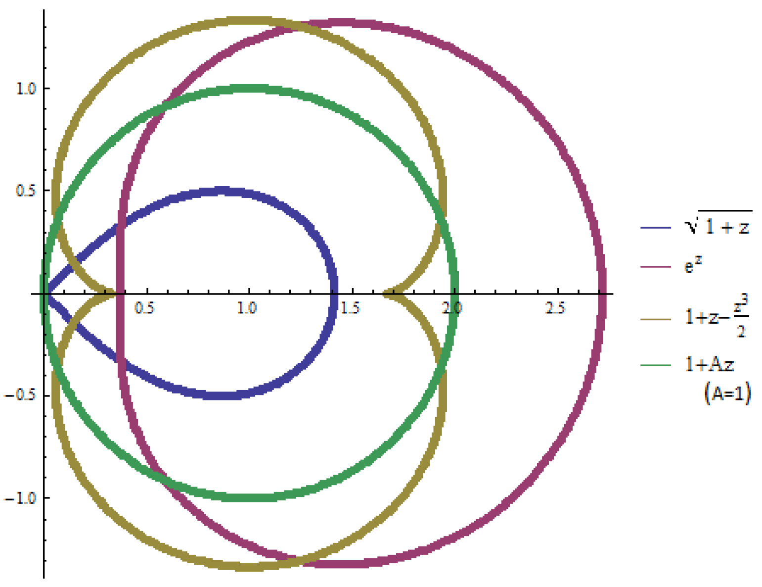
6]. Here, the leminscate domain refers to the image of D = { z : | z | < 1 } by the function P l ( z ) = 1 + z , while the image of D by the function φ N e ( z ) = 1 + z z 3 / 3 is known as nephroid domain. Two other interesting domains are the image of D by φ e ( z ) = e z , and φ A ( z ) = 1 + A z . In this article, we mainly consider P l and φ N e . The images of D through the four above functions can be seen in Figure 1 below:
Now, we recall a few basic concepts of the geometric function theory. The class of functions f defined on the open unit disk D = { z : | z | < 1 } , and normalized by the conditions f ( 0 ) = 0 = f ( 0 ) 1 , is denoted by A . We say f A 1 if f ( 0 ) = 1 is the normalized condition. Generally, f A possess power series
f ( z ) = z + n = 2 a n z n ,
while f A 1 have the power series
f ( z ) = 1 + n = 1 b n z n .
Subordination [7] is one of the important concepts of geometric function theory that is useful in studying the geometric properties of analytic functions. If f 1 and f 2 are two analytic mappings in D , then f 1 is said to be subordinate to f 2 , denoted by f 1 f 2 , or f 1 ( z ) f 2 ( z ) , z D , when there an analytic self-map η of D satisfying η ( 0 ) = 0 and | η ( z ) | < 1 exists such that f 1 ( z ) = f 2 ( η ( z ) ) , z D . In particular, if f 2 ( 0 ) = f 1 ( 0 ) with univalent f 2 , then f 1 ( D ) f 2 ( D ) .
Indicate the important sub-classes of A that comprise univalent starlike and convex functions by S * and C , respectively. For 0 t 1 , and w f ( D ) , if the line t w lies completely in f ( D ) , then f S * ; on the other hand, if f ( D ) is a convex domain, then f C . The Cárath}eodory class P includes analytic functions p that satisfy p ( 0 ) = 1 and Re p ( z ) > 0 in D . These sub-classes are related to each other. In analytical terms, f S * if z f ( z ) / f ( z ) P , and f C if 1 + z f ( z ) / f ( z ) P .
If 1 + ( z f ( z ) / f ( z ) ) is within the region bounded by the right half of the lemniscate of Bernoulli, denoted by { w : | w 2 1 | = 1 } , then the function f A is known as the lemniscate convex. This is equivalent to subordination 1 + ( z f ( z ) / f ( z ) ) 1 + z . In an analogous way, if z f ( z ) / f ( z ) 1 + z , then the function f is lemniscate starlike. Moreover, if f ( z ) 1 + z , then the function f A is lemniscate Carathéodory. It is evident that the lemniscate Carathéodory function is univalent since it is a Carathéodory function. More details about geometric properties associated with leminiscate can be seen in [5,8,9].
For the purpose of studying different classes of analytical functions, the principle of differential subordination [10,11] is helpful. Lemma 1, which is derived by applying the principle of differential subordination, is useful in sequence when studying geometric properties associated with the lemniscate.
Lemma 1 
([5]). Let p H [ 1 , n ] with p ( z ) 1 and n 1 . Let Ω C , and Ψ : C 3 × D C satisfy
Ψ ( r , s , t ; z ) Ω
whenever z D , and for m n 1 , π / 4 θ π / 4 ,
r = 2 cos ( 2 θ ) e i θ , s = m e 3 i θ 2 2 cos ( 2 θ ) and Re ( t + s ) e 3 i θ 3 m 2 8 2 cos ( 2 θ ) .
If Ψ ( p ( z ) , z p ( z ) , z 2 p ( z ) ; z ) Ω for z D , then p ( z ) 1 + z in D .
In this article, we study the geometric nature of the solution of two differential equations
z y ( z ) + a ( z ) y ( z ) + b ( z ) y ( z ) = d ( z )
z 2 y ( z ) + a ( z ) y ( z ) + b ( z ) y ( z ) = d ( z ) ;
where a ( z ) , b ( z ) , and d ( z ) are analytic functions defined on the unit disc. We find the solution of the following two problems.
Problem 1. 
Find the condition(s) on a ( z ) , b ( z ) , and d ( z ) , such that the solution f of the differential Equations (3) and (4), which are normalized by f ( 0 ) = 1 , is subordinated by 1 + z .
A few studies [1,2,3,4,12] in the literature have examined Problem 1, taking account of special a ( z ) , b ( z ) , and d ( z ) . Nonetheless, in this investigation we first present and evaluate a broad interpretation of the findings in Section 2, and then we present examples in Section 3. Below, we provides some background information:
  • Confluent hypergeometric function (CHF): This is a solution of the differential Equation (3) when a ( z ) = β z , b ( z ) = α , and d ( z ) = 0 . There are several articles in the literature that studied CHF in the context of geometric function theory [10,13]. We note here that to the best of our knowledge, there is no CHF result related to Problem 1. We established some connection between CHF and Problem 1 in the Example 1 where we also provide a detailed literature review on CHF and its connection with geometric function theory.
  • Generalized Bessel function (GBF): By taking a ( z ) = κ B , b ( z ) = c / 4 , and d ( z ) = 0 , in the differential Equation (4), we will obtain the GBF. Here, 2 κ B = 2 p + b + 1 0 , 2 , 4 , 6 , and b C . More details about GBF and its significance in the geometric functions theory are given in Example 5. A closed form of results related to Problem 1 involving GBF is given in [12].
  • Generalized Struve functions (GSF): This function is a solution of the differential Equation (4) when a ( z ) = ( 2 κ s + 1 ) / 4 , b ( z ) = ( c z + 2 κ s 2 ) / 4 , and d ( z ) = ( κ s 1 ) / 2 . Moreover, details about these notations, and the connection between GSF and Problem 1, are presented in Example 6.
  • Generalized Bessel–Sturve functions: For the construction details about this function, we refer the interested reader to [4]. A Connection of Problem 1 with this function is also studied in [4]. In Example 7, we show that the result of [4] is a special case of our main result presented in Section 2.
  • Other functions: In addition, we can consider other functions that are the solution of differential Equations (3) and (4), like the associated Laguerre polynomial (ALP) (Example 2), the regular Coulomb wave function (Example 8), generalized hypergeometric functions (Example 3), and modified Bessel functions (Example 4).
In the context of other similar geometric properties such as leminiscate starlike and convexity, we refer interested readers to [1,5,8,9,12,14] and the reference therein.
Using the solution of Problem 1, we aim to obtain the answer to the following problem.
Problem 2. 
Using the solution of Problem 1, construct functions g such that g ( z ) φ N e ( z ) .
We answer Problem 2 through various examples in Section 4.1. For this purpose, we consider the following result from [6].
Lemma 2 
([6]). Let p : D C be analytic such that p ( 0 ) = 1 . Then, the following subordinations imply p ( z ) ϕ N ϵ ( z ) :
(i)
1 + δ z p ( z ) 1 + z for δ δ 1 : = 3 ( 1 log ( 2 ) ) 0.920558 ,
(ii)
1 + δ z p ( z ) p ( z ) 1 + z for δ δ 2 : = 2 2 + log ( 2 ) 1 log ( 1 + 2 ) log ( 5 / 3 ) 0.884792 .
We also construct function f, which is subordinated by 1 + z by the direct definition of subordination and then build a connection with ϕ N ϵ . Those results are presented in Section 4.2.
In the conclusion Section 5, we raised an open problem based on the examples constructed in Section 4.

2. Subordinated by Lemniscate 1 + z

Theorem 1. 
Suppose that a ( z ) , b ( z ) , and d ( z ) are analyt
ic in D , such that the differential equation
z y ( z ) + a ( z ) y ( z ) + b ( z ) y ( z ) = d ( z )
has a solution F normalized by F ( 0 ) = 1 . Suppose that
4 Re ( a ( z ) 1 ) > 16 | b ( z ) | + 8 2 | d ( z ) | 3 ,
then F ( z ) 1 + z
Proof. 
Suppose that the second-order differential equation as given in (5) has a solution y ( z ) = F ( z ) such that F ( 0 ) = 1 . To imply Lemma 1, let us denote p ( z ) = F ( z ) . From (5), it follows that
z p ( z ) + a ( z ) p ( z ) + b ( z ) p ( z ) d ( z ) = 0 ,
which can be rewritten as
z 2 p ( z ) + a ( z ) z p ( z ) + b ( z ) z p ( z ) z d ( z ) = 0 .
Define Ψ : C 3 × D C as
Ψ ( p ( z ) , z p ( z ) , z 2 p ( z ) ; z ) : = z 2 p ( z ) + a ( z ) z p ( z ) + b ( z ) z p ( z ) z d ( z ) .
Consider Ω = { 0 } . Then, from (8) it follows that Ψ ( p ( z ) , z p ( z ) , z 2 p ( z ) ; z ) Ω . From (9), define
Ψ ( t , s , r ; z ) = t + a ( z ) s + b ( z ) z r z d ( z ) ,
By taking t = z 2 p ( z ) , s = z p ( z ) , and r = p ( z ) , rewrite (10) as below
Ψ ( t , s , r ; z ) = ( t + s ) + ( a ( z ) 1 ) s + z b ( z ) r z d ( z ) ,
and then apply Lemma 1.
For m 1 and θ [ π / 4 , π / 4 ] , it follows that
| Ψ ( t , s , r ; z ) | = | ( t + s ) + ( a ( z ) 1 ) m e 3 i θ 2 2 cos ( 2 θ ) + z b ( z ) 2 cos ( 2 θ ) e i θ z d ( z ) | | ( t + s ) + ( a ( z ) 1 ) m e 3 i θ 2 2 cos ( 2 θ ) | | z b ( z ) 2 cos ( 2 θ ) e i θ | | z d ( z ) | = | ( t + s ) e 3 i θ + ( a ( z ) 1 ) m 2 2 cos ( 2 θ ) | 2 cos ( 2 θ ) | z | | b ( z ) | | z | | d ( z ) | Re ( t + s ) e 3 i θ + Re ( a ( z ) 1 ) m 2 2 cos ( 2 θ ) 2 cos ( 2 θ ) | b ( z ) | | d ( z ) | 3 m 2 8 2 cos ( 2 θ ) + Re ( a ( z ) 1 ) m 2 2 c o s ( 2 θ ) 2 cos ( 2 θ ) | b ( z ) | | d ( z ) | = 1 8 2 cos ( 2 θ ) ( 3 m 2 + 4 m Re ( a ( z ) 1 ) 16 cos ( 2 θ ) | b ( z ) | 8 2 cos ( 2 θ ) | d ( z ) | ) = χ ( m ) 8 2 cos ( 2 θ ) .
Here,
χ ( m ) = 3 m 2 + 4 m Re ( a ( z ) 1 ) 16 cos ( 2 θ ) | b ( z ) | 8 2 cos ( 2 θ ) | d ( z ) | .
Our aim here is to show χ ( m ) > 0 for m 1 and π / 4 θ π / 4 . Since, for π / 4 θ π / 4 , c o s ( 2 θ ) [ 0 , 1 ] , it follows from (11) that
χ ( m ) 3 m 2 + 4 m Re ( a ( z ) 1 ) 16 | b ( z ) | 8 2 c o s ( 2 θ ) | d ( z ) | .
Further, for m 1 , it is always holds that m 2 2 m 1 . Along with this, let us assume that 4 Re ( a ( z ) 1 ) > 6 . Then, from (12) we have
χ ( m ) m ( 6 + 4 Re ( a ( z ) 1 ) ) 16 | b ( z ) | 8 | d ( z ) | 3 ( 6 + 4 Re ( a ( z ) 1 ) ) 16 | b ( z ) | 8 | d ( z ) | 3 > 0
provided
4 Re ( a ( z ) 1 ) > 16 | b ( z ) | + 8 | d ( z ) | 3 .
Finally, χ ( m ) > 0 if
4 Re ( a ( z ) 1 ) > max { 6 , 16 | b ( z ) | + 8 | d ( z ) | 3 } = 16 | b ( z ) | + 8 | d ( z ) | 3 .
In continuation, we have | Ψ ( t , s , r ; z ) | > 0 and hence Ψ ( t , s , r ; z ) Ω . From Lemma 1, it follows that p ( z ) = F ( z ) 1 + z . □
Theorem 2. 
Let a ( z ) , b ( z ) , and d ( z ) be analytic in D , such that the differential equation
z 2 y ( z ) + a ( z ) z y ( z ) + b ( z ) y ( z ) = d ( z )
has a solution F ( z ) satisfying F ( 0 ) = 1 . Suppose that
4 Re ( a ( z ) 1 ) > 16 | b ( z ) | + 8 2 | d ( z ) | 3 ,
then F ( z ) 1 + z .
Proof. 
Suppose that y ( z ) = F ( z ) is a solution of (13) with condition F ( 0 ) = 1 . Let p ( z ) = F ( z ) . From the differential Equation (13), it follows that
z 2 p ( z ) + a ( z ) z p ( z ) + b ( z ) p ( z ) = d ( z ) .
Now, consider Ω = { 0 } and define
Ψ ( p ( z ) , z p ( z ) , z 2 p ( z ) ; z ) : = z 2 p ( z ) + a ( z ) z p ( z ) + b ( z ) p ( z ) d ( z ) .
Then, (15) leads to Ψ ( p ( z ) , z p ( z ) , z 2 p ( z ) ; z ) Ω . From (16), define
Ψ ( t , s , r ; z ) : = t + a ( z ) s + b ( z ) r d ( z ) .
From Lemma, 1 rewrite (17) as bellow:
Ψ ( t , s , r ; z ) = ( t + s ) + ( a ( z ) 1 ) s + b ( z ) r d ( z ) = ( t + s ) + ( a ( z ) 1 ) m e 3 i θ 2 2 c o s ( 2 θ ) + b ( z ) 2 c o s ( 2 θ ) e i θ d ( z )
| Ψ ( t , s , r ; z ) | = | ( t + s ) + ( a ( z ) 1 ) m e 3 i θ 2 2 c o s ( 2 θ ) + b ( z ) 2 c o s ( 2 θ ) e i θ d ( z ) | | ( t + s ) + ( a ( z ) 1 ) m e 3 i θ 2 2 c o s ( 2 θ ) | | b ( z ) 2 c o s ( 2 θ ) e i θ | | d ( z ) | | ( t + s ) e 3 i θ + ( a ( z ) 1 ) m 2 2 c o s ( 2 θ ) | 2 c o s ( 2 θ ) | b ( z ) | | d ( z ) | Re ( t + s ) e 3 i θ + Re ( a ( z ) 1 ) m 2 2 c o s ( 2 θ ) 2 c o s ( 2 θ ) | b ( z ) | | d ( z ) |
| Ψ ( t , s , r ; z ) | 3 m 2 8 2 c o s ( 2 θ ) + Re ( a ( z ) 1 ) m 2 2 c o s ( 2 θ ) 2 c o s ( 2 θ ) | b ( z ) | | d ( z ) | = 1 8 2 c o s ( 2 θ ) 3 m 2 + 4 Re ( a ( z ) 1 ) m 16 c o s ( 2 θ ) | b ( z ) | 8 2 c o s ( 2 θ ) | d ( z ) | = χ ( m ) 8 2 c o s ( 2 θ ) ,
where χ ( m ) is the same as defined in (11). From this, the rest of the proof is similar to the proof of Theorem 1 and hence we omit the details. □
Remark 1. 
Here, it is important to observe that the identical condition makes Theorems 1 and 2 valid. However, a careful selection of a ( z ) , b ( z ) , and d ( z ) yields different sets of solutions for the differential Equations (3) and (4). In Section 3, we provide multiple examples to support this claim.

3. Examples Involving Special Functions

In this section, we are going to construct examples based on the theorems that are stated and proved in the previous section. The examples consist of several well-know special functions such as the Bessel, Struve, confluent hypergeometric, and generalized Bessel functions. The Laguerre polynomial and regular Coulomb wave functions are also covered. We refer to [15,16,17] for additional information regarding special functions.
Example 1 (Involving confluent hypergeometric functions). 
Let us consider the differential equation
z y ( z ) + ( β z ) y ( z ) α y ( z ) = 0 .
The differential Equation (18) is a well known confluent hypergeometric differential equation, and the solution of this equation is known as confluent hypergeometric functions (CHF) [15,17]. We denote the solution of (18) by ϕ ( α , β , z ) . It is also denoted as 1 F 1 ϕ ( α , β , z ) and has the series representation
ϕ ( α , β , z ) = 1 F 1 ( α , β , z ) = n = 0 ( α ) n z n ( β ) n n ! .
Here β 1 , 2 ,
In [10], Miller and Mocanu proved that Re ϕ ( α , β , z ) > 0 in D for real α and β satisfying either a > 0 and β α , or α 0 and β 1 + 1 + α 2 . Sufficient conditions for Re ϕ ( α , β , z ) > δ , 0 δ 1 / 2 are obtained by Ponnusamy and Vuorinen ([13] Theorem 1.9, p. 77). They also determined conditions that ensure ( β / α ) ϕ ( α , β , z ) 1 is close-to-convex of the positive order with respect to the identity function. Additionally, they derived the conditions for the close-to-convexity of z ϕ ( α , β , z ) with respect to the starlike function z / ( 1 z ) , as well as the close-to-convexity of z ϕ ( α , β , z ) with respect to the starlike function z / ( 1 z 2 ) . Constraints on a and c so that ϕ ( α , β , z ) is convex of the positive order are also found in ([13] Theorem 5.1, p. 88).
Now, we are going to implement Theorem 1 in the solution f 1 ( z ) = ϕ ( α , β , z ) of differential Equation (18). Note that a ( z ) = β z , b ( z ) = α and d ( z ) = 0 .
We consider the case where α C and
Re { β 1 } > 4 | α | + 1 4 .
Now,
4 Re ( a ( z ) 1 ) 16 | b ( z ) | + 3 = 4 Re ( β z 1 ) 16 | α | + 3 = 4 Re ( β 1 ) 4 Re ( z ) 16 | α | + 3 > 4 Re ( β 1 ) 4 16 | α | + 3 = 4 Re ( β 1 ) 16 | α | 1 > 0 .
Thus, condition (6) holds and we have the following result from Theorem 1:
Theorem 3. 
For α , β C , the confluent hypergeometric function ϕ ( α , β , z ) 1 + z for
Re { β 1 } > 4 | α | + 1 4 .
Example 2 (Involving the Laguerre polynomial). 
The associated Laguerre polynomial (ALP) denoted by L n α ( z ) is the solution of the differential equation
z y ( z ) + ( α + 1 z ) y ( z ) + n y ( z ) = 0 , α R .
The function L n α ( z ) can be represented by the series
L n α ( z ) = i = 0 n ( 1 ) i n + α n i z i i ! = ( 1 + α ) n n ! 1 F 1 ( n ; 1 + α ; z ) ,
where 1 F 1 represents the confluent hypergeometric function, and ( a ) n denotes the familiar Pochhammer symbol defined as
( a ) 0 = 1 , ( a ) n = a ( a + 1 ) ( a + n 1 ) , n N .
We refer to [15] for further information on this function.
Consider the normalized function
F α , n ( z ) = n ! ( α + 1 ) n L n α ( z ) = 1 F 1 ( n ; 1 + α ; z ) , z D .
The function F α , n satisfies the normalization condition F α , n ( 0 ) = 1 . Thus, from Theorem 3, it follows that
F α , n ( z ) 1 + z
provided 4 Re ( α ) > 16 n + 1 . It is to be noted here that this result is the main result of the article ([2] Theorem 1). The result ([2] Theorem 1) obtained by considering the differential equation
z 2 y ( z ) + ( α + 1 z ) z y ( z ) + n z y ( z ) = 0 , α R ,
which follows from (20) by multiplying z on both sides. Thus, the result can also be obtained from Theorem 2.
Before introducing the next example, we first recall generalized hypergeometric functions denoted by
m F n ( a 1 , a 2 , , a m ; b 1 , b 2 , , b n ; z )
with series representation
m F n ( a 1 , a 2 , , a m ; b 1 , b 2 , , b n ; z ) = r = 0 ( a 1 ) r ( a 2 ) r ( a m ) r ( b 1 ) r ( b 2 ) r ( b n ) r z n n !
where b i , 1 i n are positive. The series (25) converges if
(i)
Any of a j , 1 j m are non-positive.
(ii)
m < n + 1 , the series converges for any finite value of z and hence entirely.
Let m = 0 and n = 1 ; then, the generalized hypergeometric function 0 F 1 ( ; a ; z ) is known as confluent hypergeometric finite functions, and this function is closely related to the Bessel function as follows:
Γ ( v + 1 ) J v ( z ) = z 2 v 0 F 1 ; v + 1 ; z 2 4 Γ ( v + 1 ) I v ( z ) = z 2 v 0 F 1 ; v + 1 ; z 2 4 .
Next, we provide an example involving the generalized hypergeometric function.
Example 3 (Involving generalized hypergeometric functions). 
Consider the function
f 3 ( z ) = e z 2 0 F 1 ; 3 ; 3 z 2 .
Clearly, f 3 ( 0 ) = 1 . By taking the differentiation on both sides, we have
f 3 ( z ) = 3 2 e z 2 0 F 1 ; 3 ; 3 z 2 + 1 2 e z 2 0 F 1 ; 3 ; 3 z 2
The relation
d d z 0 F 1 ( ; a ; z ) = 0 F 1 ( ; a + 1 ; z ) a ,
implies
f 3 ( z ) = 1 2 e z 2 0 F 1 ; 4 ; 3 z 2 + 1 2 e z 2 0 F 1 ; 3 ; 3 z 2 = 1 2 e z 2 0 F 1 ; 3 ; 3 z 2 0 F 1 ; 4 ; 3 z 2
similarly,
f 3 ( z ) = 1 16 e z 2 4 0 F 1 ; 3 ; 3 z 2 8 0 F 1 ; 4 ; 3 z 2 + 3 0 F 1 ; 5 ; 3 z 2
z f 3 ( z ) + ( 3 z ) f 3 + z 4 f 3 ( z ) = e z 2 z 4 0 F 1 ; 3 ; 3 z 2 z 2 0 F 1 ; 4 ; 3 z 2 + 3 z 16 0 F 1 ; 5 ; 3 z 2 + ( 3 z ) 1 2 0 F 1 ; 3 ; 3 z 2 1 2 0 F 1 ; 4 ; 3 z 2 + z 4 0 F 1 ; 3 ; 3 z 2 = e z 2 z 4 + 3 2 z 2 + z 4 0 F 1 ; 3 ; 3 z 2 + z 2 3 2 + z 2 0 F 1 ; 4 ; 3 z 2 + 3 z 16 0 F 1 ; 5 ; 3 z 2 = 3 2 e z 2 0 F 1 ; 3 ; 3 z 2 + 0 F 1 ; 4 ; 3 z 2 + z 8 0 F 1 ; 5 ; 3 z 2
Again, the recurrence relation
0 F 1 ( ; a ; z ) = 0 F 1 ( ; a + 1 ; z ) + z a ( a + 1 ) 0 F 1 ( ; a + 2 ; z )
implies
0 F 1 ; 3 ; 3 z 2 = 0 F 1 ; 4 ; 3 z 2 z 8 0 F 1 ; 5 ; 3 z 2 ,
and this leads to the fact that f 3 is a solution of the differential equation
z f 3 ( z ) + ( 3 z ) f 3 ( z ) + z 4 f 3 ( z ) = 0 .
Now, to implement Theorem 1, let us consider
a ( z ) = 3 z , b ( z ) = z 4 , and d ( z ) = 0 .
Since z D , we have 1 < Re ( z ) < 1 and | z | < 1 . Trivially, Re ( a ( z ) 1 ) > 0 . Finally, a calculation yields
4 Re ( 3 z 1 ) 16 z 4 + 3 = 11 4 Re ( z ) 4 | z | > 11 4 Re ( z ) 4 = 11 8 = 3 > 0 .
This means that a ( z ) , b ( z ) , and d ( z ) satisfy the requirement of Theorem 1; hence, we conclude that f 3 ( z ) 1 + z .
Example 4 (Involving classical modified Bessel functions). 
Consider the function
f 4 ( z ) = 1 6 e z 8 ( 6 + z ) I 0 z 8 + ( 2 + z ) I 1 z 8 .
Here, I v is a well-known modified Bessel function that is the solution of the differential equation
z 2 y ( z ) + z y ( z ) ( z 2 + v 2 ) y ( z ) = 0
and have the series representation
I v ( z ) = z v 2 v n = 0 z 2 n 4 n n ! Γ ( v + v + 1 ) = z v 2 v 1 Γ ( v + 1 ) + z 2 4 Γ ( v + 2 ) +
clearly,
I 0 ( 0 ) = 1 , I 1 ( 0 ) = 0
Thus,
f ( 0 ) = 1 6 e 0 ( 6 I 0 ( 0 ) + 2 I 1 ( 0 ) = 1 .
Our objective here is to find the corresponding differential equation of f 4 . Various well-known recurrence relations of modified Bessel functions help us to establish the differential equation. We recall the following recurrence relations of I ν :
I v ( z ) = I v + 1 ( z ) + v z I v ( z )
2 I v ( z ) = I v 1 ( z ) + I v + 1 ( z ) .
A calculation from (27) and (28) yields
I ν + 1 ( z ) = I v 1 ( z ) 2 v z I v ( z ) .
For ν = 0 , the recurrence relation (27) gives
I 0 z 8 = 1 8 I 1 z 8
Further, the recurrence relations (28) and (29) leads to
I 1 z 8 = 1 16 I 0 z 8 + I 2 z 8 = 1 16 2 I 0 z 8 16 z I 1 z 8 .
Using above relation and several adjustment, one can obtain
f 4 ( z ) = 1 12 e z 8 I 0 z 8 + 1 4 z I 1 z 8 ,
and
f 4 ( z ) = 1 24 z 2 e z 8 z I 0 z 8 ( z 16 ) I 1 z 8 .
Now, a combination of (26), (30), and (31) leads to
z f 4 ( z ) + 2 + z 4 f 4 ( z ) 1 8 f 4 ( z ) = 1 24 z e z 8 z I 0 z 8 ( z 16 ) I 1 z 8 + 2 + z 4 1 12 e z 8 I 0 z 8 + 1 4 z I 1 z 8 1 8 1 6 e z 8 ( 6 + z ) I 0 z 8 + ( 2 + z ) I 1 z 8 = e z 8 1 24 I 0 z 8 1 24 1 16 z I 1 z 8 + 1 6 + z 48 I 0 z 8 + 1 12 2 z 4 1 4 z I 1 z 8 1 48 ( 6 + z ) I 0 z 8 1 48 ( 2 + z ) I 1 z 8 = 0 .
Thus, f 4 ( z ) is the solution of the differential equation
z y ( z ) + 2 + z 4 y ( z ) 1 8 y ( z ) = 0 .
Taking
a ( z ) = 2 + z 4 , b ( z ) = 1 8 , d ( z ) = 0 ,
it follows that
4 Re ( a ( z ) 1 ) 16 | b ( z ) | + 3 = 4 Re ( 2 + z 4 1 ) 16 1 8 + 3 = Re ( z ) + 5 > 0 .
Finally, from Theorem 1, one can conclude that f 4 ( z ) 1 + z .
Example 5 (Involving generalized Bessel functions). 
In the literature on geometric functions theory, one of the most important functions is the generalized and normalized Bessel functions of the form
U p ( z ) = n = 0 ( 1 ) n c n 4 n ( κ B ) n z n n ! , 2 κ B = 2 p + b + 1 0 , 2 , 4 , 6 , ;
which satisfies the second-order differential equation
4 z 2 U ( z ) + 4 κ B z U ( z ) + c z U ( z ) = 0 .
The function U p yields the Spherical Bessel function for b = 2 , c = 1 and reduces to the normalized classical Bessel (modified) Bessel functions of order p when b = c = 1 ( b = c = 1 ).
There is an extensive amount of research on the inclusion of U p in different subclasses of univalent functions theory [12,18,19,20,21,22] and some references therein. In [12], the lemniscate convexity and additional properties of U p are examined in detail. The lemniscate starlikeness of z U p is discussed in [1].
From the differential Equation (33), it follows that a ( z ) = κ B , b ( z ) = c / 4 , and d ( z ) = 0 . The condition (14) is equivalent to
4 Re ( κ B 1 ) 16 c z 4 + 3 > 0 4 Re ( κ B 1 ) 4 | c | + 3 > 0 Re ( κ B ) > | c | + 1 4 .
Thus, we have the following result.
Theorem 4. 
If Re ( κ B ) > | c | + 1 / 4 , then U p ( z ) 1 + z .
Baricz [18] proved that the following recurrence relation is satisfied by U p as follows:
Lemma 3 
([18]). If b , p , c C and κ 0 , 1 , 2 , , then the function U p ( z ) satisfies the relation 4 κ B U p ( z ) = c U p + 1 for all z C .
Now, Theorem 4 and Lemma 3 together imply that for c 0 and Re ( κ B ) > | c | 3 / 4 ,
4 κ B c U p ( z ) 1 + z .
The subordination in (34) is established in [12] with the condition Re ( κ B ) > max { 0 , | c | 3 / 4 } .
Example 6 (Involving Generalized Struve functions). 
For p , z C , consider the function
H p ( z ) = n = 0 ( 1 ) n Γ n + 3 2 Γ p + n + 3 2 z 2 2 n + p + 1 .
The function H p is well known as the Struve function of order p, and it is a particular solution of the non-homogeneous differential equation
z 2 w ( z ) + z w ( z ) + ( z 2 p 2 ) w ( z ) = 4 ( z / 2 ) p + 1 π Γ ( p + 1 / 2 ) .
A slightly modified differential equation
z 2 w ( z ) + z w ( z ) ( z 2 + p 2 ) w ( z ) = 4 ( z / 2 ) p + 1 π Γ ( p + 1 / 2 )
has a particular solution of the form
L p ( z ) = i exp i p π / 2 H p ( i z ) = n 0 1 Γ ( n + 3 / 2 ) Γ ( p + n + 3 / 2 ) z 2 2 n + p + 1 .
The function L p is known as a modified Struve function of order p. The notion of generalized Struve functions is given in [23]. The starlikeness and convexity properties of generalized Struve functions also studied in [24].
Now, let us consider the second-order non-homogeneous linear differential equation.
z 2 w ( z ) + b z w ( z ) + ( c z 2 p 2 + ( 1 b ) p ) w ( z ) = 4 ( z / 2 ) p + 1 π Γ ( p + b / 2 )
where b , c , p C . If we choose b = 1 and c = 1 , then we obtain (35), and if we choose b = 1 and c = 1 , then we obtain (36). So, this generalizes (35) and (36). Hence, the study based on (37) helps us to study the Struve and modified Struve functions together. Now, the particular solution of the differential Equation (37) is known as a generalized Struve function of order p and denoted by w p , b , c ( z ) . The generalized struve function w p , b , c ( z ) is represented by the following series:
w p , b , c ( z ) = n 0 ( 1 ) n c n Γ ( n + 3 / 2 ) Γ ( p + n + ( b + 2 ) / 2 ) z 2 2 n + p + 1 , z C
While this series converges everywhere, the function w p , b , c ( z ) typically is not univalent within D . Now, let us examine the function S p , b , c ( z ) defined by the transformation
S p , b , c ( z ) = 2 p π Γ p + b + 2 2 z ( p 1 ) / 2 w p , b , c ( z )
By using the Pochhammer symbol, which is defined in relation to Euler’s gamma functions, by ( λ ) n = Γ ( λ + n ) / Γ ( λ ) = λ ( λ + 1 ) ( λ + n 1 ) , we obtain for the function S p , b , c ( z ) in the following form:
S p , b , c ( z ) = n = 0 ( c / 4 ) n ( 3 / 2 ) n ( κ s ) n z n ,
where κ s = p + ( b + 2 ) / 2 0 , 1 , 2 .This function is analytic on C and satisfies the second-order non-homogeneous differential equation
4 z 2 u ( z ) + ( 2 κ s + 1 ) z u ( z ) + ( c z + 2 κ s 2 ) u ( z ) = 2 κ s 2 .
From differential Equation (39), it follows that a ( z ) = ( 2 κ s + 1 ) / 4 , b ( z ) = ( c z + 2 κ s 2 ) / 4 and d ( z ) = ( κ s 1 ) / 2 . Now, to satisfy the condition (14), we have to show
4 Re 1 4 ( 2 κ s + 1 ) 1 16 1 4 ( c z + 2 κ s 2 ) 8 2 1 2 ( κ s 1 ) 3 > 0 .
Since | z | < 1 , a simplification of right hand side of (40) gives
4 Re 1 4 ( 2 κ s + 1 ) 1 16 1 4 ( c z + 2 κ s 2 ) 8 2 1 2 ( κ s 1 ) 3 > Re 2 κ s 3 4 | c | 4 ( 2 + 2 ) | κ s 1 | + 3 .
Thus, the inequality (40) holds if Re 2 κ s 3 4 ( 2 + 2 ) | κ s 1 | > 4 | c | 3 , and by this we have the conclusion S p , b , c ( z ) 1 + z .
Example 7 (Involving the generalized Bessel–Sturve function). 
The concept of the generalized Bessel–Sturve function is introduced in [4], building upon the concepts of the generalized Struve function S ν , b , c from [23] and the generalized Bessel function J ν , b , c from article [18]. By denoting the generalized Bessel–Sturve functions as BS ν , b , c ( z ) , it is shown in [4] that for ν > 1 / 2 , the generalized Bessel–Sturve functions exhibit a power series of the form:
BS ν , b , c ( z ) = n = 0 ( c ) n / 2 Γ n + 1 2 π n ! Γ ( n 2 + κ ) z n w h e r e κ B S = ν + ( b + 1 ) / 2 .
Further, it is established in ([4] Proposition 2) that BS ν , b , c is a solution of the differential equation
z 2 F ( z ) + ( 2 κ 1 ) z F ( z ) c z 2 F ( z ) = N z ,
where c C and N = 2 c Γ ( κ B S ) / π Γ κ B S 1 2 .
Now, to apply Theorem 2, set
a ( z ) = 2 κ B S 1 , b ( z ) = c z 2 , and d ( z ) = z N .
The condition (14) is equivalent to
4 Re ( 2 κ B S 2 ) 16 | c z 2 | 8 2 | z N | + 3 > 0 .
Since | z | < 1 , it follows that
4 Re ( 2 κ B S 2 ) 16 | c z 2 | 8 2 | z N | + 3 > 8 Re ( κ B S 1 ) 16 | c | 8 2 | N | + 3 .
Substituting the expression for N , it follows that
4 Re ( 2 κ B S 2 ) 16 | c z 2 | 8 2 | z N | + 3 > 8 Re ( κ B S 1 ) 16 | c | 8 2 | N | + 3 = 8 Re ( κ B S 1 ) 16 | c | 8 2 2 c Γ ( κ B S ) π Γ ( κ B S 1 2 ) + 3 .
Finally, the condition (43) holds if
π Γ ( κ B S 1 2 ) 8 Re ( κ B S 1 ) 16 | c | + 3 16 2 Γ ( κ B S ) | c | .
The inequality (44) help us to conclude that BS ν , b , c ( z ) 1 + z . A similar result is also obtained in [4].
Example 8 (Involving the regular Coulomb wave function). 
The regular Coulomb wave function ( R C W F ) , defined across the complex plane, is an entire function linked to the classical Bessel function. The Coulomb differential equation is a secound-order differential equation of the form
d 2 w d z 2 + 1 2 η z L ( L + 1 ) z 2 w = 0 , z , η , L C
claiming two distinct solutions: the regular and irregular Coulomb wave functions. The regular Coulomb wave function ( R C W F ) is expressed in terms of the Kummer confluent hypergeometric function 1 F 1 as follows:
F L , η ( z ) : = z L + 1 e i z C L ( η ) 1 F 1 ( L + 1 + i η , 2 L + 2 ; 2 i z ) = C L ( η ) n = 0 a L , n z n + L + 1 .
In this case, z , η , L C and
C L ( η ) = 2 L e π η 2 | Γ ( L + 1 + i η ) | Γ ( 2 L + 2 ) , a L , 0 = 1 , a L , 1 = η L + 1 , a L , n = 2 η a L , n 1 a L , n 2 n ( n + 2 L + 1 ) , n { 2 , 3 , . } .
For our requirement, we consider the following normal form:
f L ( z ) = C L 1 ( η ) z L 1 F L , η ( z ) = 1 + η L + 1 z + . . . . .
By a calculation, it can be shown from (45) that f L satisfies the differential equation
z 2 y ( z ) + 2 ( L + 1 ) z y ( z ) + ( z 2 2 η z ) y ( z ) = 0 , z , η , L C
a ( z ) = 2 ( L + 1 ) , b ( z ) = z 2 η z , d ( z ) = 0 .
For condition (14), the conclusion of this results follows if
4 Re ( 2 L + 2 1 ) > 16 | z 2 2 η z | 3 4 Re ( 2 L + 1 ) 16 | z 2 2 η z | + 3 > 0 .
Now, due to the fact that | z 1 + z 2 | | z 1 | + | z 2 | and | z 1 | < 1 , we have
4 Re ( 2 L + 1 ) 16 | z 2 2 η z | + 3 4 Re ( 2 L + 1 ) 16 | z 2 | 32 | η | | z | + 3 = 4 Re ( 2 L + 1 ) 13 32 | η | > 0 ,
provided Re ( 2 L + 1 ) > 13 4 + 8 | η | , and due to this inequality it is always true that Re ( a ( z ) 1 ) = Re ( 2 L + 1 ) > 0 . Now, from Theorem 2, it follows that f L ( z ) 1 + z . We remark here that this result is obtained in ([3] Theorem 1).

4. Connections with Nephroid Domain

In this section, we investigate the functions that map the unit disk to a domain confined by the nephroid curve. We are going to generate appropriate cases in two ways: first, by employing some of the examples established in Section 3, and second, by taking into consideration the idea of subordination. Suppose that f A such that f ( 0 ) = 1 and f ( z ) 1 + z . Define
g ( z ) : = 1 + 1 δ 0 z f ( t ) 1 t d t ,
and assume that the integration on the right-hand side is convergent. From (48), it follows by the fundamental theorem of calculus that
g ( z ) = f ( z ) 1 δ z 1 + δ z g ( z ) = f ( z ) 1 + z .
From Lemma 2 (i), it follows that g ( z ) φ N e ( z ) , for δ δ 1 .
Denote h ( z ) : = e g ( z ) 1 . A logarithmic differentiation of h yields
h ( z ) h ( z ) = f ( z ) 1 β z 1 + β z h ( z ) h ( z ) = f ( z ) 1 + z .
Again by Lemma 2 (ii), it follows that h ( z ) φ N e ( z ) for β β 2 .
Lemma 4. 
If f ( z ) 1 + z , then the following two subordinations are true:
g ( z ) = 1 + 1 δ 0 z f ( t ) 1 t d t φ N e ( z ) and h ( z ) = e g ( z ) 1 φ N e ( z ) .
Now, we can construct the functions g in two ways. In the first method, we can consider constructed functions f in various examples in Section 3 and calculate the integration (48), while in the second method, we will directly construct a function f 1 + z using the definition of subordination. Before constructing more examples in this direction, we state the following theorem, which directly follows from the relationship between (49) and Theorems 1 and 2. We omit the proof.
Theorem 5. 
Consider the analytic functions a ( z ) , b ( z ) , and d ( z ) defined on D such that the conditions of Theorems 1 and 2 holds. Then, for δ δ 1 , g ( z ) φ N e ( z ) where g is the solution of any of the following two differential equations:
z 2 y ( z ) + ( 2 + a ( z ) ) z y ( z ) + ( a ( z ) + z b ( z ) ) y ( z ) = d ( z ) b ( z ) δ z 3 y ( z ) + ( 2 + a ( z ) ) z 2 y ( z ) + ( a ( z ) + b ( z ) ) z y ( z ) = d ( z ) b ( z ) δ .

4.1. Examples Based on Section 3

To construct examples in connection with φ N e ( z ) , we first revisit Section 3 where the connections with 1 + z are presented.
Example 9. 
In Example 5, we prove that for Re ( κ ) > | c | + 1 / 4 , the generalized Bessel function U p ( z ) < 1 + z . Now, from the series (32) of U p , it follows that
u p ( t ) 1 t = n = 1 ( 1 ) n c n 4 n ( κ ) n n ! t n 1 .
Define
g p ( δ , z ) = 1 + 1 δ 0 z u p ( t ) 1 t d t .
Then, we have g ( δ , p , z ) φ N e ( z ) for δ > δ 1 provided integration (50) exists. Our next aim is to find the closed form of g ( δ , p , z ) .
g p ( δ , z ) = 1 + 1 δ n = 1 ( 1 ) n c n 4 n ( κ ) n n ! 0 z t n 1 d t = 1 + 1 δ n = 1 ( 1 ) n c n 4 n ( κ ) n n ! z n n = 1 c z 4 κ δ n = 0 ( 1 ) n c n z n 4 n ( κ + 1 ) n ( n + 1 ) ! ( n + 1 ) = 1 c z 4 κ δ n = 0 ( 1 ) n c n z n ( 1 ) n 4 n ( κ + 1 ) n ( 2 ) n ( 2 ) n = 1 c z 4 κ δ 1 F 3 1 , 1 ; 2 , 2 , κ + 1 ; c z 4
This concludes the following subordination:
  • 1 c z 4 κ δ 1 F 3 1 , 1 ; 2 , 2 , κ + 1 ; c z 4 φ N e ( z ) for δ > δ 1 ,
  • e x p c z 4 κ δ 1 F 3 1 , 1 ; 2 , 2 , κ + 1 ; c z 4 φ N e ( z ) for δ > δ 2 .
Example 10. 
In Example 4, we prove that
f ( z ) = 1 6 e z / 8 ( 6 + z ) I 0 z 8 + ( 2 + z ) I 1 z 8 1 + z
Then,
g ( δ , z ) = 1 + 1 δ 0 z f ( t ) 1 t d t = 1 + 1 δ 0 z 1 6 e t / 8 ( 6 + t ) I 0 t 8 + ( 2 + t ) I 1 t 8 1 t d t = 1 + e z / 8 3 δ ( 3 + z ) I 0 z 8 ( 1 z ) I 1 z 8 1 8 δ 8 + z 3 F 3 1 , 1 , 3 2 ; 2 , 2 , 2 ; z 4 .

4.2. Examples Using Definition of Subordination

The next few examples are constructed directly using the definition of subordination.
Example 11. 
For δ > 0 and | a | 1 , consider the function
G 1 ( δ , a , z ) : = 1 + 2 δ 1 + a z ln ( 1 + 1 + a z ) 1 + ln ( 2 )
To establish the subordination, consider the function w ( z ) = a z with | a | 1 . Then, clearly W ( 0 ) = 1 , and for z D , | w ( z ) | = | a | | z | < | a | 1 . By the definition of subordination, the relation 1 + a z = 1 + w ( z ) implies 1 + a z 1 + z .
For δ > 0 and | a | 1 , define
G 1 ( δ , a , z ) : = 1 + 1 δ 0 z f ( t ) 1 t d t ,
with f ( t ) = 1 + a t .
The solution of the integration in (52) can be easily established using computational software, but here we solve the problem to achieve the completeness of the result. First, we consider the following indefinite integration:
I = f ( t ) 1 t d t = 1 + a t 1 t d t = 1 + a t 1 1 + a t + 1 t 1 + a t + 1 d t = a 1 + a t + 1 d t .
Next, substitute r = 1 + a t . Then,
d r = a 2 1 + a t d t a d t = 2 r d r .
The integration I reduces to
I = 2 r r + 1 d r = 2 1 1 r + 1 d r = 2 r 2 ln | r + 1 | + c 1 = 2 1 + a t 2 ln ( 1 + 1 + a t ) + c 1 .
Finally, the integration (52) has the closed form
G 1 ( δ , a , z ) = 1 + 1 δ 0 z 1 + a t 1 t d t = 1 + 1 δ 2 1 + a t 2 ln ( 1 + 1 + a t ) 0 z = 1 + 2 δ 1 + a z ln ( 1 + 1 + a z ) 1 + ln ( 2 ) .
From Lemma 4, it follows that
G 1 ( δ , a , z ) = 1 + 2 δ 1 + a z ln ( 1 + 1 + a z ) 1 + ln ( 2 ) φ N e ( z ) ,
for δ > δ 1 .
Example 12. 
In this example, we show that for δ > δ 1 the function
G 2 ( δ , z ) : = 1 + 1 3 δ 1 z 5 + z 6 ln ( 1 + 1 z ) + l n ( 64 ) 5 φ N e ( z ) .
Let us consider the function
w ( z ) = 3 z 2 4 z 3 4 = z 2 4 ( 3 + z ) .
Clearly, w ( 0 ) = 0 and for | z | < 1
| w ( z ) | = | z | 2 4 3 + z < 1 .
Further, we have
1 + w ( z ) = 1 3 4 z 2 z 3 4 = ( 1 z ) 1 + z + z 2 4 = ( 1 z ) 1 + z 2 2 .
Using the definition of differential subordination, we conclude that
1 z 1 + z 2 1 + z .
Now, if we define
G 2 ( δ , z ) = 1 + 1 δ 0 z 1 t 1 + t 2 1 t d t ,
then by Lemma 4, we can conclude that g 2 ( δ , z ) φ N e ( z ) for δ > δ 1 . It remains to find a closed form of g 2 ( δ , z ) that is subject to the existence of the integration in (56).
To check this, first we consider the indefinite integration
I 1 = 1 t 1 + t 2 1 t d t ,
which can be further separated into two parts as follows:
I 1 = 1 t 1 t d t + 1 2 1 t d t .
Taking a = 1 in (53), we have the solution of the first integration in I 1 as
1 t 1 t d t = 2 1 t 2 ln ( 1 + 1 t ) + c 1 .
By a routine calculation, the second integration in I 1 leads to
1 t d t = 2 3 ( 1 t ) 3 / 2 + c 2 .
This finally leads to the closed form of g 2 as follows:
G 2 ( δ , z ) = 1 + 1 δ 0 z 1 t 1 + t 2 1 t d t = 1 + 1 δ 2 1 t 2 ln ( 1 + 1 t ) 1 3 ( 1 t ) 3 2 0 z = 1 + 1 δ 2 1 z 2 ln ( 1 + 1 z ) 1 3 ( 1 z ) 3 2 + l n ( 4 ) 5 3 = 1 + 1 3 δ 1 z 5 + z 6 ln ( 1 + 1 z ) + l n ( 64 ) 5 .
This completes the verification.
Example 13. 
In this example, we show that for δ > δ 1 , the function
G 3 ( δ , z ) : = 1 + 1 δ 47 30 + 1 60 1 z ( 94 + 17 z + 9 z 2 ) 2 ln ( 1 + 1 z ) + ln ( 4 ) φ N e ( z ) .
To establish this, we consider the following two functions:
f ( z ) = 1 z 1 + z 2 + 3 z 2 8 w ( z ) = z 3 64 ( 9 z 2 + 15 z + 40 ) .
Clearly, w ( 0 ) = 0 and
| w ( z ) | = z 3 ( 9 z 2 + 15 z + 40 ) 64 = | z | 3 ( 9 | z | 2 + 15 | z | + 40 ) 64 < ( 9 + 15 + 40 ) 64 = 1 .
Further, a computation yields
( 1 z ) 1 + z 2 + 3 z 2 8 2 = 1 + w ( z ) .
This gives us required subordination
1 z 1 + z 2 + 3 z 2 8 1 + z .
Similarly to the earlier examples, let us define
G 3 ( δ , z ) = 1 + 1 δ 0 z 1 t 1 + t 2 + 3 t 2 8 1 t d t
Since
1 t ( 1 + t 2 + 3 8 t 2 ) 1 t = 1 t 1 t + 1 2 1 t + 3 8 t 1 t ,
the integration in (59) can be evaluated as follows:
G 3 ( δ , z ) = 1 + 1 δ 0 z 1 t 1 + t 2 + 3 t 2 8 1 t d t = 0 z 1 t 1 t d t + 1 2 0 z 1 t + 3 8 0 z t 1 t d t = 2 1 t 2 ln ( 1 + 1 t ) 1 3 ( 1 t ) 3 2 1 20 ( 1 t ) 3 2 ( 2 + 3 t ) 0 z = 1 60 1 z ( 94 + 17 z + 9 z 2 ) 2 ln ( 1 + 1 z ) + ln ( 4 ) 47 30 .
The conclusion follows from Lemma 4.

5. Conclusions

In this article, we state and prove two results that gave conditions on the analytic coefficient of the second-order differential equation by which the solution of the differential equation maps the unit disk to a domain subordinate to the leminscate 1 + z and the nephroid curve φ N e ( z ) . In consequence, several examples involving special functions such as Bessel, Struve, Bessel–Sturve, the confluent, and generalized hypergeometric functions are presented. Based on the construction pattern of G i , i = 1 , 2 , 3 in Section 4.2, we have the following open problem:
Problem 3. 
For a fixed n N { 0 } , construct a sequence { a k } k = 1 n and define the polynomial P 0 ( z ) = 1 , and P n ( z ) = 1 + k = 1 n a k z k for n 1 . Find the exact range of a, such that
1 + a z P n ( z ) 1 + z .
Further, for δ > δ 1 , the function
G i ( δ , a , z ) = 1 + 1 δ 0 z 1 + a t P i 1 ( t ) 1 t d t φ N e ( z ) , i = 1 , 2 , ,
provided the integration converge.
We note that
(i)
Example 11: n = 0 , | a | < 1 and P 0 = 1 ,
(ii)
Example 12: n = 1 , a = 1 and P 1 ( z ) = 1 + z 2
(iii)
Example 13: n = 2 , a = 1 and P 2 ( z ) = 1 + z 2 + 3 z 2 8 .
Thus, Examples 11–13 partially answer Problem 3. Now, from the pattern of the above three examples and Problem 3, we can observe the following specific problem:
Problem 4. 
For a fixed n N { 0 } , define the polynomial
P 0 ( z ) = 1 P n ( z ) = 1 + k = 1 n 2 k 1 2 2 k 1 z k for n 1 .
Then, some a R { 0 } exist such that
1 + a z P n ( z ) 1 + z .

Author Contributions

Conceptualization, R.A. and S.R.M.; methodology, R.A. and S.R.M.; validation, R.A. and S.R.M.; formal analysis, R.A. and S.R.M.; investigation, R.A. and S.R.M.; writing—original draft preparation, R.A.; writing—review and editing, S.R.M.; and supervision, S.R.M. All authors have read and agreed to the published version of the manuscript.

Funding

This work was supported by the Deanship of Scientific Research, Vice Presidency for Graduate Studies and Scientific Research, King Faisal University, Saudi Arabia (Grant No. 5120).

Data Availability Statement

Data are contained within the article.

Conflicts of Interest

The authors declare no conflicts of interest.

References

  1. Mondal, S.R. On Lemniscate Starlikeness of the Solution of General Differential Equations. Mathematics 2022, 10, 3254. [Google Scholar] [CrossRef]
  2. Mondal, S.R. Mapping Properties of Associate Laguerre Polynomials in Leminiscate, Exponential and Nephroid Domain. Symmetry 2022, 14, 2303. [Google Scholar] [CrossRef]
  3. Mondal, S.R. Subordination Involving Regular Coulomb Wave Functions. Symmetry 2022, 14, 1007. [Google Scholar] [CrossRef]
  4. Alarifi, N.M.; Mondal, S.R. On Geometric Properties of Bessel–Sturve Kernel Functions in Unit Disc. Mathematics 2022, 10, 2516. [Google Scholar] [CrossRef]
  5. Madaan, V.; Kumar, A.; Ravichandran, V. Starlikeness associated with lemniscate of Bernoulli. Filomat 2019, 33, 1937–1955. [Google Scholar] [CrossRef]
  6. Swaminathan, A.; Wani, L.A. Sufficiency for nephroid starlikeness using hypergeometric functions. Math. Methods Appl. Sci. 2022, 45, 5388–5401. [Google Scholar] [CrossRef]
  7. Duren, P.L. Univalent Functions. In Grundlehren der Mathematischen Wissenschaften [Fundamental Principles of Mathematical Sciences]; Springer: New York, NY, USA, 1983; Volume 259, pp. xiv+382. [Google Scholar]
  8. Ali, R.M.; Cho, N.E.; Ravichandran, V.; Sivaprasad Kumar, S. Differential subordination for functions associated with the lemniscate of Bernoulli. Taiwanese J. Math. 2012, 16, 1017–1026. [Google Scholar] [CrossRef]
  9. Kumar, S.S.; Kumar, V.; Ravichandran, V.; Cho, N.E. Sufficient conditions for starlike functions associated with the lemniscate of Bernoulli. J. Inequal. Appl. 2013, 2013, 176. [Google Scholar] [CrossRef]
  10. Miller, S.S.; Mocanu, P.T. Differential subordinations and inequalities in the complex plane. J. Differ. Equ. 1987, 67, 199–211. [Google Scholar] [CrossRef]
  11. Miller, S.S.; Mocanu, P.T. Differential subordinations Theory and applications. In Monographs and Textbooks in Pure and Applied Mathematics; Marcel Dekker, Inc.: New York, NY, USA, 2000; Volume 225, pp. xii+459. [Google Scholar]
  12. Madaan, V.; Kumar, A.; Ravichandran, V. Lemniscate convexity of generalized Bessel functions. Studia Sci. Math. Hungar. 2019, 56, 404–419. [Google Scholar] [CrossRef]
  13. Ponnusamy, S.; Vuorinen, M. Univalence and convexity properties for confluent hypergeometric functions. Complex Var. Theory Appl. 1998, 36, 73–97. [Google Scholar] [CrossRef]
  14. Yadav, S.; Ravichandran, V. Analytic function that map the unit disk into the inside of the lemniscate of Bernoulli. Math. Found. Comput. 2023, 6, 1–10. [Google Scholar] [CrossRef]
  15. Abramowitz, M.; Stegun, I.A. Handbook of Mathematical Functions with Formulas, Graphs, and Mathematical Tables; US Government Printing Office: Washington, DC, USA, 1968; Volume 55. [Google Scholar]
  16. Andrews, G.E.; Askey, R.; Roy, R. Special Functions—Encyclopedia of Mathematics and its Applications; Cambridge University Press: Cambridge, UK, 1999; Volume 71, pp. xvi+664. [Google Scholar] [CrossRef]
  17. Temme, N.M. Special Functions: An Introduction to the Classical Functions of Mathematical Physics; A Wiley-Interscience Publication; John Wiley & Sons, Inc.: New York, NY, USA, 1996; pp. xiv+374. [Google Scholar] [CrossRef]
  18. Baricz, A. Generalized Bessel Functions of the First Kind; Lecture Notes in Mathematics; Springer: Berlin, Geramny, 2010; Volume 1994, pp. xiv+206. [Google Scholar] [CrossRef]
  19. Baricz, A.; Ponnusamy, S. Starlikeness and convexity of generalized Bessel functions. Integral Transform. Spec. Funct. 2010, 21, 641–653. [Google Scholar] [CrossRef]
  20. Baricz, A.; Szász, R. The radius of convexity of normalized Bessel functions of the first kind. Anal. Appl. 2014, 12, 485–509. [Google Scholar] [CrossRef]
  21. Baricz, A. Geometric properties of generalized Bessel functions. Publ. Math. Debrecen 2008, 73, 155–178. [Google Scholar] [CrossRef]
  22. Baricz, A. Geometric properties of generalized Bessel functions of complex order. Mathematica 2006, 48, 13–18. [Google Scholar]
  23. Orhan, H.; Yagmur, N. Geometric properties of generalized Struve functions. An. Ştiinţ. Univ. Al. I. Cuza Iaşi. Mat. (N.S.) 2017, 63, 229–244. [Google Scholar] [CrossRef]
  24. Yagmur, N.; Orhan, H. Starlikeness and convexity of generalized Struve functions. Abstr. Appl. Anal. 2013, 6, 954513. [Google Scholar] [CrossRef]
Figure 1. Image of | z | = 1 by φ N e ( D ) , P L ( D ) , φ A = 1 ( D ) , and φ e ( D ) .
Symmetry 16 00019 g001
Disclaimer/Publisher’s Note: The statements, opinions and data contained in all publications are solely those of the individual author(s) and contributor(s) and not of MDPI and/or the editor(s). MDPI and/or the editor(s) disclaim responsibility for any injury to people or property resulting from any ideas, methods, instructions or products referred to in the content.

