Maintaining Symmetry between Convolutional Neural Network Accuracy and Performance on an Edge TPU with a Focus on Transfer Learning Adjustments

Abstract

Transfer learning has proven to be a valuable technique for deploying machine learning models on edge devices and embedded systems. By leveraging pre-trained models and fine-tuning them on specific tasks, practitioners can effectively adapt existing models to the constraints and requirements of their application. In the process of adapting an existing model, a practitioner may make adjustments to the model architecture, including the input layers, output layers, and intermediate layers. Practitioners must be able to understand whether the modifications to the model will be symmetrical or asymmetrical with respect to the performance. In this study, we examine the effects of these adjustments on the runtime and energy performance of an edge processor performing inferences. Based on our observations, we make recommendations for how to adjust convolutional neural networks during transfer learning to maintain symmetry between the accuracy of the model and its runtime performance. We observe that the edge TPU is generally more efficient than a CPU at performing inferences on convolutional neural networks, and continues to outperform a CPU as the depth and width of the convolutional network increases. We explore multiple strategies for adjusting the input and output layers of an existing model and demonstrate important performance cliffs for practitioners to consider when modifying a convolutional neural network model.

1. Introduction

Convolutional neural networks (CNNs) are a powerful tool for solving a variety of problems using deep learning techniques, demonstrating an exceptional performance in tasks such as image classification, object detection, and segmentation. Their ability to automatically learn hierarchical features from raw data has revolutionized various industries, from healthcare to autonomous vehicles. However, training deep CNNs from scratch demands vast amounts of labeled data and computational resources, making applying them difficult for many real-world applications.

Transfer learning addresses this challenge by leveraging models that are pre-trained on large datasets and adapting them for specific tasks with limited labeled data. This approach not only significantly reduces the data requirements but also accelerates convergence during training. During the process of applying transfer learning to a CNN, a practitioner may wish to tweak the neural network architecture to further fit the targeted application. Changes to the neural network architecture may affect both the accuracy of the network and the runtime performance of the network executing on a device, and it is important for practitioners to be able to maintain symmetry between accuracy and performance.

To address the intensive computational needs of neural networks, Google introduced the tensor processing unit (TPU), a specialized chip tailored for machine learning applications [1]. The TPU relies on a matrix multiply unit, enabling parallel processing. Initially designed for data centers [2] with an emphasis on performance rather than energy efficiency, the original TPU paved the way for subsequent developments. Subsequently, the Coral edge TPU emerged as a low-power alternative, specifically crafted for embedded systems and on-device machine learning inference. The term edge denotes its capacity to operate autonomously without depending on cloud servers, processing data locally instead. While it may not match the speed of Google’s original Cloud TPU, the Coral edge TPU excels in on-device machine learning applications. Its ability to capture, analyze, and process data at the source, rather than offloading it for external processing, proves to be beneficial for various applications, such as IoT security [3], wildlife behavior monitoring [4], and signal noise reduction [5].

For the experiments detailed in this paper, we employed Google’s edge TPU. Specifically, our experimentation involved the use of the Coral Development (Dev) Board, a comprehensive platform that integrates a TPU alongside a CPU, sensors, and various devices tailored for edge machine learning applications. Figure 1 illustrates our setup, comprising a Linux-operating laptop, a Gen7i data acquisition system [6], two external power supplies, and the Coral Dev Board. The primary focus of our analysis in this paper revolves around assessing the runtime performance and energy consumption of the edge TPU in comparison to a mobile CPU. We conducted these evaluations across a range of neural network models, aiming to illuminate the strengths and weaknesses of the edge TPU.

We evaluated the performance of the edge TPU compared to a mobile CPU with specific interest in convolutional neural networks that have been modified as part of the process of transfer learning. We started by evaluating the runtime and energy performance of the edge TPU compared to the mobile CPU on a set of baseline convolutional neural networks. We then evaluated modified versions of a subset of the convolutional neural networks to model the tweaks that might be made by a practitioner during the process of applying transfer learning.

This paper makes the following contributions:

• Proposes a methodology for determining the limits of neural network performance on edge devices;
• Analyzes the performance, both runtime and energy, of an edge TPU on both fully connected and convolutional neural networks as compared to a mobile CPU;
• Assesses the performance impact of modifications made to convolutional neural networks as part of transfer learning;
• Provides recommendations for how symmetry between accuracy and performance can be maintained throughout transfer learning adjustments.

The remainder of this paper is organized as follows. Section 2 presents background material and related work on deep neural networks and tensor processors. Section 3 discusses the methodology for our experiments. Section 4 presents the results of the experiments that we conducted. Section 5 provides practical recommendations for neural network designs targeting edge tensor processors. Finally, Section 6 concludes the paper.

2. Background and Related Work

In the following sections, we discuss the relevant background on neural network architectures and tensor processing units. We also highlight related work.

2.1. Deep Neural Networks

Deep neural networks offer promise as flexible, nearly “off-the-shelf” solutions to machine learning problems that can perform adequately even for non-expert users or those who lack significant technical domain knowledge [7,8]. By using deep neural networks, less experienced practitioners can apply machine learning to their domain-specific problem. Common deep neural network structures include fully connected neural networks and convolutional neural networks.

Neural networks (a.k.a. artificial neural networks) are a type of machine learning model inspired by the biological neurons in the human brain [9]. They comprise multiple layers of interconnected nodes, known as neurons, that work together to process information and make predictions. In a feed-forward neural network, information flows in one direction, from the input layer through one or more hidden layers, to the output layer. In a fully connected feed-forward neural network, each neuron in a layer receives input from all of the neurons in the previous layer, performs a calculation using weights and biases, and then passes the result to the neurons in the next layer. By adjusting the weights and biases of the neurons, the network can learn to recognize patterns in data and make accurate predictions. Fully connected neural networks have been successfully applied to a wide range of tasks, including image recognition, speech recognition, and natural language processing.

Convolutional neural networks (CNNs) are a type of deep (i.e., large number of layers) neural network model that excels at image processing tasks [10], among others. The name convolutional comes from the use of convolutional kernels. A kernel is feature map that represents each node in a given layer as its weighted inputs from the same number and arrangement of neurons in the previous layer. In other words, the inputs to each node differ only by the shifting of a common weight vector (and bias term) at the previous layer. CNNs were inspired by the way the visual cortex in the brain processes visual information. A typical CNN consists of multiple layers of interconnected neurons, including convolutional layers, pooling layers, and fully connected layers. For an image processing CNN, in a convolutional layer, a set of filters is applied to the input image, the effect of which is to extract features such as edges and textures. The output of the convolutional layer can then be passed through a pooling layer to reduce the dimensionality of the features and make the model more efficient. Finally, the output of the pooling layer is typically fed into one or more fully connected layers, which perform classification or regression on the extracted features. CNNs have been shown to be very effective at a variety of image processing tasks, including object recognition, face detection, and image segmentation. They have also been applied in other domains such as natural language processing and speech recognition.

2.2. Transfer Learning

Transfer learning is a technique used in machine learning where a pre-trained model serves as a starting point for training a model for a new task [11]. Rather than starting from scratch, which requires significant computation and large amounts of labeled training data, a pre-trained model is fine-tuned to the new task by updating its weights and biases using a smaller dataset. The intuition behind transfer learning is that the features learned by the pre-trained model on a large dataset are likely to be useful for a new, related task, even if the input datasets are not identical in nature. In transfer learning, either only the new parts of the model or the entire model can be retrained (with weights initialized per the original application) [12] depending on the training time requirements. Many domains have successfully applied transfer learning. It is particularly useful when there are limited labeled data available for the new task or when training from scratch would take too long.

Transfer learning is commonly performed by replacing the input and output layers of the pre-trained model with layers that fit the target problem. SpinalXNet [13] adds a specialized fully connected layer to the end of the ResNet-101 model to identify COVID-19 in X-ray images. Other approaches use transfer learning with a modified ResNet architecture to detect emotion in crowds [14] and brain tumors [15,16]. A modified version of the VGG-16 model is used with transfer learning to detect solar flares [17]. In similar work, modified versions of the AlexNet, ResNet50, DenseNet161, and VGG-16 models were used with transfer learning to detect Leukemia in blood smear images [18]. Modified versions of AlexNet and SqueezeNet were used to classify radar jamming signals [19]. In all of these examples, transfer learning is used to reduce the requirements for training data and training time.

Small changes may also be made to the existing model in an attempt to improve accuracy on the target problem. To identify diseases in potato leaves [20], the VGG19, NASNetMobile, and DenseNet169 models are modified to increase the width and depth of the original models and are used with transfer learning to reduce the number of parameters that must be trained. CNNs have also been extended with additional layers to make the model deeper to classify pulmonary nodules [21]. A shallow version of the Inception model was used to diagnose Alzheimer’s disease [22]. Deeper and wider CNNs have been evaluated for a variety of computer-aided detection algorithms with transfer learning [23]. A modified Inception model has been used with transfer learning to recognize ancient architectures [24]. Prior work has even investigated making models deeper by concatenating two models [25].

Overall, motivation exists from prior work on transfer learning for examining the performance implications of transfer learning techniques that modify the input layers, output layers, and even the base model.

2.3. Tensor Processing

Tensor processing units (TPUs) represent specialized hardware designed explicitly for neural networks, featuring meticulous optimization for matrix multiplication [1,26,27,28]. This specificity grants TPUs a notable edge over CPU and GPU architectures in terms of speed, accompanied by minimal power consumption. In a comparative analysis with the Haswell CPU and NVIDIA K80 GPU, TPUs demonstrated the lowest power usage per die, albeit with the highest energy per area. Conversely, the CPU exhibited the highest power consumption but showcased superior energy proportionality.

When scrutinizing performance per watt, TPUs excelled, exhibiting a 14–16 times improvement over the NVIDIA K80 GPU and an impressive 17–34 times advantage over the Haswell CPU [1]. Furthermore, there have been algorithms proposed that aim to leverage the embedded processor by operating at a lower voltage and frequency, all while preserving runtime performance, further enhancing the versatility of TPUs [27].

The core function of the edge TPU in conducting inferences through neural networks centers around matrix processing. Therefore, the chip design features thousands of multiply-accumulate units in a so-called systolic array [2]. In contrast, a CPU, even with vector instructions, can only execute a small number of add or multiply instructions per cycle. For convolutional neural networks, which generally require a large number of multiply-adds per inference, the TPU architecture greatly accelerates the computation.

The Coral edge TPU can perform around four trillion operations per second at the cost of 0.5 W for each tera-operation per second [26,28]; this efficiency enables on-device AI computations. Benchmarking assessments conducted on the Coral Dev board, across diverse model architectures, reveal a substantial superiority of on-board TPU inference times over its CPU counterpart. The performance gap ranges from a minimum of five times faster, extending up to an impressive 100 times faster for specific network models [26,29].

Other machine learning accelerators, including the NVIDIA Jetson [30], Intel Movidius [31], and Qualcomm Snapdragon [32], provide hardware support similar to the Google edge TPU. A recent survey [33] reviewed the features and performance of embedded machine learning accelerators. Although the exact structures of these devices may differ, they all accelerate the multiply-add operations that are common to neural network computations using batch operations on layer inputs, weights, and biases. Due to finite computational units and memory, all of these devices will experience performance cliffs as the input and weight sizes exceed the hardware limitations. We chose the Coral TPU as a representative device for this study.

2.4. Related Work

Given the high interest in edge machine learning, prior work has studied the performance of edge tensor processors. In [28], the authors evaluate the performance of convolutional networks from the NASBench-101 benchmark suite on three edge tensor processors with the goal of training a performance and energy model for exploring new tensor processor architectures. The paper evaluates 423,000 unique convolutional neural network models on three edge tensor processors. In a similar study [34], the authors evaluate fully connected and convolutional neural networks to predict performance and power on an edge TPU. The authors find that multiply-add operations and memory usage can be used to estimate power and performance with less than 10% error. DeepEdgeBench [29] evaluates five edge processors on the MobileNetV2 benchmark. In [35], the authors evaluate the performance of a set of CNNs on the NVIDIA Jetson. In [36], the authors perform a similar study on the NVIDIA Jetson Nano with a focus on providing accurate power measurements on that device for Deep Neural Networks. In another related paper [37], the authors examine the performance of individual operations on the NVIDIA Jetson Xavier and Nano processors on Deep Neural Networks.

Our work differs from these prior studies by generating modified network models based on real-world examples and evaluating the performance impact of transfer learning techniques. Prior work examines specific CNN models and does not consider the types of modifications that are made to CNN models as part of transfer learning. Specifically, it is important to assess the performance impact of modifications to the input and output layers.

Prior work has also evaluated the performance of edge tensor processors in the context of specific applications, including network intrusion detection [38,39], animal activity classification [40], object classification [41,42], and smart greenhouse development [43]. In a comprehensive survey [33], the authors summarize the use of embedded machine learning processors, including the Coral TPU, for sensing applications. Our work does not examine any specific applications because the accuracy of a machine learning model in a specific domain may vary wildly depending on the availability of training data, the availability of powerful training hardware, and the ability to select appropriate training parameters.

Finally, a large amount of prior work has been done on building better edge processors [44,45,46,47,48,49,50,51,52]. Our work does not aim to inform the design of new hardware for machine learning but rather to provide insights and an evaluation methodology for developing machine learning models for edge tensor processors.

3. Methodology

We conducted measurements to evaluate both the runtime performance and energy usage of the Coral edge TPU across a range of convolutional neural network architectures. Our comparative analysis involved assessing the runtime performance of the Coral edge TPU against the mobile CPU integrated into the Coral development board. For more detail on the specifications of these devices, refer to

Table 1. Comparison of the processors studied in these experiments.

	Coral TPU [53]	Coral CPU [53,54]
Processor	Google Edge TPU	Cortex-A53 Quad-core
Frequency	480 MHz	3.01 GHz
RAM	4 GB DDR4	4 GB DDR4
Operation Type	Fixed Point	Floating Point
Operations/s	4 Trillion (8-bit)	32 Billion (32-bit)

.

We recorded the runtime of the interpreter.invoke() function provided by the tflite-runtime Python library using Python’s built-in time.perf_counter_ns() function to produce runtime performance data. The performance measurement conducted focuses on the runtime performance of inferences using the machine learning model. Across all experiments, we meticulously recorded the runtime for 10,000 inferences, and the results are presented as the average runtime for a single inference in each graph. The experiments were executed using Python version 3.7.3 and tflite-runtime version 2.5.0. All scripts used in this study are available on Github (https://github.com/crdelozier/cnn_symmetry (accessed on 8 January 2024)).

In our energy measurements, the Coral development board was supplied with power through a 5 volt, 3 amp power source. To gauge energy consumption accurately, we connected the ground pin through a 0.1-ohm resistor to a Gen7i data acquisition system, which incorporates a high-resolution oscilloscope (as seen in Figure 1). The Gen7i data system samples the voltage across the resistor at a rate of 100 kHz. The data acquisition system begins taking samples based on a trigger from a GPIO pin on the development board that is set to high just prior to invoking the inference. The GPIO pin is set to low as soon as the inference ends. The energy required to complete an inference, E, is calculated as shown in (1), where $v_S$ indicates supply voltage, R indicates resistance, $v_R$ indicates voltage across the resistor, $f_s$ indicates sampling rate, and K indicates the duration, in samples, required to complete the inference.

$$E=\sum _{k=1}^K(v_S{v}_R\left[k\right]-v_R^2\left[k\right])\frac{1/f_s}{R}.$$

(1)

Figure 2 shows sample voltage traces for the CPU and TPU on the MobileNet1.0 convolutional neural network. These traces are processed using a Matlab script that outputs the total energy (J) recorded during the inference.

3.1. Convolutional Neural Networks

For baseline experiments on convolutional neural networks, we started with a set of CNN models, described in

Table 2. Characteristics of baseline CNN models. FNN240L810N is provided as a comparison point for fully connected networks.

Model Name	Input	Output	GFLOP	Layers	% Parallel Layers
EfficientDet320 [56]	320 × 320 × 3	90	2323.1	266	36%
EfficientDet384 [56]	384 × 384 × 3	90	4272.3	321	31%
EfficientDet448 [56]	448 × 448 × 3	90	6806.7	356	29%
EfficientDet512 [56]	512 × 512 × 3	90	13,117.4	423	29%
EfficientDet640 [56]	640 × 640 × 3	90	23,671.8	423	29%
EfficientNetS [57]	244 × 244 × 3	1000	2991.1	66	0%
EfficientNetM [57]	240 × 240 × 3	1000	4598.3	86	0%
EfficientNetL [57]	300 × 300 × 3	1000	11,752.0	97	0%
InceptionV1 [58]	244 × 244 × 3	1000	2167.2	83	53%
InceptionV2 [59]	244 × 244 × 3	1000	2708.2	98	46%
InceptionV3 [59]	299 × 299 × 3	1000	7347.8	132	47%
InceptionV4 [60]	299 × 299 × 3	1000	15,666.1	205	32%
MobileDetSSDLite [61]	320 × 320 × 3	90	2437.3	136	32%
MobileDetV1 [62]	300 × 300 × 3	90	1929.1	75	44%
MobileDetV2Coco [61]	300 × 300 × 3	90	1494.4	110	30%
MobileDetV2Face [61]	320 × 320 × 3	90	1524.6	132	25%
TF2MobileDetV1 [63]	640 × 640 × 3	90	67,482.4	104	56%
TF2MobileDetV2 [63]	300 × 300 × 3	90	1407.5	101	24%
DLV3DM05MobileNet [64]	513 × 513 × 3	20	2276.7	72	0%
DLV3MobileNet [64]	513 × 513 × 3	20	5343.5	72	0%
KerasMobileNet128 [65]	128 × 128 × 3	37	1350.8	76	10%
KerasMobileNet256 [65]	256 × 256 × 3	37	5390.1	76	10%
MobileNet0.25 [62]	128 × 128 × 3	1000	37.8	31	0%
MobileNet0.5 [62]	160 × 160 × 3	1000	155.1	31	0%
MobileNet0.75 [62]	192 × 192 × 3	1000	412.1	31	0%
MobileNet1.0 [62]	224 × 224 × 3	1000	912.6	31	0%
MobileNetV2Bird [61]	224 × 224 × 3	900	652.3	65	0%
MobileNetV2Plant [61]	224 × 224 × 3	2000	658.6	65	0%
MobileNetV2 [61]	224 × 224 × 3	1000	652.3	66	0%
TF2MobileNetV1 [63]	224 × 224 × 3	1000	840.3	33	0%
TF2MobileNetV2 [63]	224 × 224 × 3	1000	614.8	68	0%
TF2MobileNetV3 [63]	224 × 224 × 3	1000	1280.9	79	0%
FNN240L810N [66]	100 × 1	9	565.3	242	0%

, built for the edge TPU [55]. These models use deep neural networks to assist in image classification, object detection, and semantic segmentation. Many of these models are modified versions of the same base models: EfficientNet, Inception, and MobileNet.

Table 2 provides metrics that give insight into the performance impact of performing an inference with these neural networks. GFLOP shows the total number of floating point operations required to execute the model. GFLOP indicates how much total work must be performed by a processor to perform an inference, from input to output, with each model. We calculated the floating-point operations per model by executing the model, profiling the runtime per layer, and multiplying the runtime by the floating-point operations per second for the processor. GFLOP is not a perfect analog of the total runtime required to perform an inference with each model because, as shown in Figure 3, models differ in terms of how many layers can be executed in parallel throughout the model. For example, the MobileNet1.0 computes an inference using a serial chain of layers, while the InceptionV1 model computes an inference using multiple layers in parallel. These parallel layers may use different filters to extract different characteristics from the input data. The amount of parallel work in a model also depends on the sizes of the inputs, filters, and other parameters for each layer. For their Cloud TPUs, Google recommends tiling data into 128 × 8 chunks [67]. If the computation does not exactly fit that chunk size, the compiler will pad the tensors to match. This can lead to increases in the amount of memory required to store a tensor.

The Layers column shows the total number of high-level Tensorflow operations performed by each model, and the % Parallel Layers column shows the number of these operations, or layers, that can be executed in parallel. We calculated the number of parallel layers by traversing the graph and counting the steps required to execute the entire graph under the assumption that if the inputs to a layer were ready, the layer could be executed. We note that this calculation assumes an infinitely large matrix multiplication unit that can fit the entire calculations required for multiple layers concurrently. For example, in Figure 3, the InceptionV1 model could execute as follows. First, the MaxPool2D layer executes. Once the MaxPool2D layer finishes, the next three Conv2D operations and the next MaxPool2D operation can execute in parallel using the output from the first MaxPool2D layer. At this point, the output from the leftmost chain is ready for the Concatenation operation, but the rest of its inputs are not ready, so it must wait. The three remaining Conv2D operations can execute, and, finally, the Concatenation operation can execute once all of its inputs are ready. In total, the nine layers in this part of the model will execute in four steps. Therefore, we would calculate that this part of the model has $(9-4)/9=55.6\%$ parallel layers. In Table 2, we see that the total % Parallel Layers for InceptionV1 is slightly lower, at 53%, because other parts of the model have less parallel work available. We also note that speculative execution techniques may be able to exploit additional parallelism not considered by this calculation.

In combination, the Layers and % Parallel Layers columns indicate how deep or wide the baseline models are. A deeper model requires more serial steps to perform an inference. For example, MobileNet1.0 requires 31 steps, and EfficientDet320 requires $266\times 0.36\approx 96$ steps. Therefore, we would consider EfficientDet320 to be a deeper model than MobileNet1.0. A wider model performs more work per step. This can be derived from both % Parallel Layers, which shows how many of the layers can be executed in parallel, and by dividing GFLOP by Layers to find, on average, how many floating-point operations are performed per layer. For example, DLV3MobileNet is wider than DLV3DM05MobileNet because it requires more floating-point operations for the same number of total layers, which indicates that the layers must perform more work. This difference is due to the use of 2× larger filters in DLV3MobileNet.

Overall, the baseline models that we examined cover a variety of input and output sizes, total number of floating-point operations required to perform an inference, and model architectures in terms of serial versus parallel work. As a reference point, we also provide these metrics for a fully connected feed-forward neural network with 240 layers and 810 nodes per layer (FNN240L810N). In general, performing an inference with this feed-forward network requires fewer floating-point operations and has less parallel work available, compared to the CNN models.

3.2. Exploring Adjustments to CNN Models

We analyzed the structure of the CNN models to identify common modifications to produce different versions of the same model. In many cases, the baseline model features a repeated subgraph of convolution operations, as shown in Figure 4. Deeper versions of the model repeat this subgraph in order to extend the model. Wider versions of the model add convolution or other operations to the subgraph. Aside from additional convolutions, models may also add a fully connected layer at the end of the CNN.

Starting with a subset of the CNN models, we generated deeper, wider, and otherwise modified versions of these CNN models to evaluate the performance impact of such modifications. For our experiments, we used the EfficientNetS, InceptionV1, and MobileNet1.0 models as a baseline.

3.2.1. Extracting the Baseline Models from Tensorflow Lite

To create deeper and wider CNNs for performance analysis, we first needed to extract the baseline models into a modifiable format because pre-existing Tensorflow Lite models, the model format required by the edge TPU, are not easy to modify. In practice, a model designer will generate a Tensorflow Lite model from a Tensorflow model or by converting from another model format. We extract a modifiable model from the Tensorflow Lite model in two steps. First, we run Analyzer.analyze from the Tensorflow Lite Python library to extract the model architecture. This tool provides both the order and types of layers in the model and the input and output tensor sizes for each layer. However, this tool does not provide all of the required information to reproduce the model, including the filter sizes and strides. Next, we run flatc, which is the FlatBuffer compiler, to produce a json file with specific model parameters, including filters and strides. We combine these two sources of information in a Python script that generates a new model using Keras to match the input Tensorflow Lite model. For each extracted model, we verified that the extracted model’s performance and energy characteristics match the original model.

3.2.2. Generating Deeper Models

Once we had the extracted model, we created deeper models by identifying the main repeated subgraph within the original model and further repeating that subgraph. We created shallower models by removing repetitions of the subgraph. In practice, both the shallow and deep versions of each model were created in a single run of our Python script that removed all of the repeated subgraphs from the original model and then re-added one subgraph at a time to generate models with zero to N repeated subgraphs.

To create shallower and deeper versions of these models, we used the subgraphs shown in Figure 3. In EfficientNetS, the main subgraph is a 2D convolution that is added to the result of two further 2D convolutions. The main subgraph in IncepionV1 performs parallel 2D convolutions with different filter sizes. In one of the parallel branches, a 2D max pooling operation is performed. For MobileNet1.0, the main subgraph is a 2D convolution followed by a depthwise 2D convolution.

3.2.3. Generating Wider Models

We explored multiple avenues for generating wider models from the baseline CNNs by both increasing the number of layers that could be executed in parallel and increasing the work performed per layer.

To increase the number of layers, we drew inspiration from the evolution of the Inception model from InceptionV1 to InceptionV4. Figure 4 shows the main subgraph of InceptionV4. InceptionV1, InceptionV2, and InceptionV3 all use portions of this subgraph. Each layer in the subgraph attempts to derive additional information from the data by using different bias and filter sizes.

For experiments on increasing the number of parallel layers, we created wide versions of the EfficientNetS and MobileNet1.0 models because these models have 0% parallel layers in the original model. We did not expand the other baseline model from previous experiments (InceptionV1) using this methodology because it already has multiple parallel layers. We expanded existing 2D convolution layers in the numerical order shown in Figure 4. To further explain, the baseline version of the model only had the original 2D convolution (1). The first expansion of the layer adds two 2D convolutions in parallel with the original 2D convolution (2). The second expansion adds a chain of four 2D convolutions in parallel (3). The third expansion adds an average pooling operation followed by a 2D convolution (4). Finally, additional expansions add parallel layers in the two middle subgraphs (5+ and 6+).

We also examined the performance impacts of scaling up the the work performed per layer by expanding the dimensions of the 2D convolutions throughout the baseline models. We attempted to align these experiments with common transfer learning techniques. First, we widened the model at two points: after the input layer and before the output layer. We also performed an experiment with wider layers at both the input and output layers. Second, we scaled up the width of the entire model. We performed these experiments on all three of the baseline models (EfficientNetS, MobileNet1.0, and InceptionV1).

4. Experimental Results

We experimentally analyzed the execution time and energy usage of the CPU and TPU on convolutional neural networks. We first examine the runtime and energy performance of the baseline CNNs on the CPU and TPU and characterize the performance based on the structure of the network. We then examine the performance impact of modifications to a set of CNNs that might be applied to a model as part of the process of transfer learning. We examine transformations such as the input and output sizes, adding a fully connected layer after the input, and making the models deeper and wider. In particular, we look for symmetry and asymmetry between the modifications to the model and the resulting performance. All experiments were performed on the Coral edge TPU development board.

4.1. Convolutional Neural Networks

We measured the execution time of the edge CPU and edge TPU using the baseline models described in Table 2. Figure 5 shows the runtime speedup for a single inference on the Coral development board compared to the single core baseline. The baseline measurement was performed on a single CPU core. We then measured the execution time on an inference using four CPU cores and the TPU. As shown, the TPU consistently outperforms the CPU, even with four CPU cores, on all of the CNN models. The rightmost bars (geomean) show the geometric mean of all speedups for the 4-core CPU and the TPU. On average, these CNNs execute an inference on the 4-core CPU in 33% of the time it takes to execute the same model on a 1-core CPU. On the TPU, it takes 10% of the time it takes to execute the same model on a 1-core CPU.

We also compared energy per inference for the CNN models. The results of this experiment are shown in Figure 6. The energy results are similar to the runtime results for the CNN models, with the TPU consistently outperforming both the 1-core and 4-core CPUs. One notable difference is that the 4-core CPU only uses 45% less energy to perform an inference than the 1-core CPU. Given that the 4-core CPU executes an inference in 33% of the time it take to execute on the 1-core CPU, the power consumption of four cores slightly outweighs the runtime speedup from running on four cores. However, the significant improvement in runtime performance still leads to lower energy usage per inference. In low-power environments, using a 1-core CPU will provide better long-term energy usage if inferences are being run frequently. The TPU uses 10% of the energy required to perform an inference on the 1-core CPU.

Figure 7 breaks down the performance speedup of the TPU over the single core CPU with reference to the floating-point operations per parallel layer for each model. In general, more available parallel work leads to a larger performance improvement on the TPU. There are a few outliers in behavior. The DLV3DM05MobileNet and DLV3MobileNet models are outliers in the MobileNet set of models because they use operations that are not supported on the edge TPU. The RESIZE_BILINEAR function is not supported, and operations on more than one subgraph are not supported. In total, these two models use eight operations that are not supported by the TPU and must therefore run on the CPU, leading to lower performance gains on the TPU. The Inception models all have similar speedup over the CPU despite more available parallel work in the InceptionV3 and InceptionV4 models. The larger Inception models use significant amounts of off-chip memory, 5.11 MB and 36.3 MB, respectively. The increase in off-chip memory used limits the performance speedup on the TPU. Likewise, the EfficientDet640 model uses 7.72 MB of off-chip memory, which causes it to be a bit of an outlier in the EfficientNet group. Aside from these outliers, the models tend to exhibit larger speedups on the TPU compared to the CPU as the amount of parallel work available increases.

Other hardware factors may also prevent this speedup from being monotonic compared to the available parallel work. The TPU’s matrix multiplication unit may not be completely utilized at all times due to the fixed hardware structure (128 × 128 on TPU version 3) and various sizes of filters used in these CNNs. Furthermore, the TPU must load model parameters from memory, which takes additional time, especially for larger models. Other hardware factors, such as cache line sizes, associativity, and prefetching, may also impact performance. Overall, we find that floating-point operations per parallel layer is a reasonable, though certainly not perfect, indicator of the runtime performance of a CNN on the edge TPU.

4.2. Transfer Learning

Transfer learning involves applying an existing model, potentially with small modifications, to a new problem. This may require modifying the input and output layers to match the new problem’s inputs and outputs. In some cases, practitioners may wish to make small modifications to the existing model to improve its accuracy on the new problem. We are interested, specifically, in the runtime performance impact on inferences performed with modified CNN models. We do not evaluate the accuracy of such models or the impact on training time. In the following sections, we evaluate the runtime performance metrics of modifications that might be made to a model while applying transfer learning on the edge TPU.

4.3. Input and Output Size

Transfer learning often requires changing the input size of the machine learning model to match the target problem’s input characteristics. We perform two experiments to assess the performance impact of modifying the input size. For problems with image inputs, we simply vary the size of the input by resizing the image. We chose to scale the image inputs by factors of 2 (0.25×, 0.5×, 1×, 2×, and 4×). Figure 8 shows the performance impact of resizing the input images to the CNN models. As the image input size grows, the TPU speedup over the CPU decreases.

For problems with one-dimensional inputs, we apply a fully connected layer to expand the number of input parameters to more closely match the expected number of inputs from an image. We then reshape the one-dimensional data into two-dimensional data with three channels. Finally, we resize the shaped inputs to match the expected image size for the model. Figure 9 demonstrates this procedure. With powerful enough hardware to train the models, it may be possible to skip the resize operation and simply reshape the output of the fully connected layer. On our hardware, we were unable to produce a working Tensorflow Lite model with a fully connected layer that could be reshaped to the 224 × 224 × 3 input of the models (224 × 224 × 3 = 150,528 nodes in the fully connected layer).

Table 3. TPU Speedup over CPU on CNN model execution with a fully connected layer to expand input size. All models expect a 224 × 224 × 3 image input.

Model	TPU Speedup (14 FC Nodes)	TPU Speedup (224 FC Nodes)
EfficientNet	33.0×	0.99×
Inception	17.9×	0.94×
MobileNet	13.3×	0.85×

shows the speedup of the TPU over the CPU on the CNN models using a fully connected layer to expand the 1D inputs into the 2D image size expected by the CNN. As shown, with a small fully connected layer, the performance benefit of the TPU on a CNN outweighs the work required to execute the fully connected layer. As the size of the fully connected layer increases, the CPU begins to outperform the TPU, despite the TPU’s performance advantage on the CNN.

Figure 10 shows the on-chip and off-chip memory assigned to parameters for the MobileNet CNN model with a fully connected layer of size N used to expand the 1D inputs into a 2D image. For this experiment, we explored fully connected input sizes of M, where $14\le M\le$ 50,176 and the original CNN input size is 224 × 224 × 3. These bounds were derived from the original input size of 224 × 224 × 3 using $14\approx \sqrt{224}$ and 50,176 = 224 × 224. We compiled each generated model with the edgetpu compiler and recorded the amount of memory used for on-chip and off-chip model parameters. For up to 900 nodes in the fully connected layer, the edgetpu compiler uses only on-chip memory. At 3025 nodes in the fully connected layer, we notice the first instance in which the edgetpu compiler only uses off-chip memory for model parameters. In the graph, we can see that this phenomenon occurs semi-regularly when the on-chip memory falls to zero and there is a sharp spike in the off-chip memory. Within this size range, a small increase in layer size may cause a large increase in off-chip memory used, demonstrating the asymmetry caused by performance cliffs. Above 32,041 fully connected nodes, the edgetpu compiler no longer uses on-chip memory for model parameters. In short, it may be beneficial to test multiple potential sizes for a fully connected layer to determine which fits best into on-chip memory.

4.3.1. Depth Extensions

To further evaluate the performance implications of transfer learning on an edge TPU, we generated altered CNNs, based on the original models for EfficientNet, Inception, and MobileNet, with more or fewer subgraphs of the main computational component of the network. Figure 4 demonstrates the main subgraph of InceptionV1. For each of the three models, we identify the main subgraph, extract that subgraph, and generate models with 1 to 50 repetitions of that subgraph. Each of the generated models also reproduces the rest of the original model.

Figure 11 shows the results of this experiment. As shown, the performance gap between the CPU and TPU decreases as the subgraph is repeated more, but the gap remains at over 10× on these CNN models. On both the CPU and the TPU, adding repeated subgraphs may be a potential avenue to improve the accuracy of the model for a problem in transfer learning without significantly impacting performance. The difference between the worst performing and best performing generated models on the TPU was 2.5×, 4.7×, and 2.24×, respectively, for EfficientNetS, InceptionV1, and MobileNet1.0. For the CPU, the difference between the worst performing and best performing generated models was 1.06×, 1.15×, and 1.38×, respectively. We expect that cache locality and data transfer explain the CPU’s relative efficiency as the depth of the model increases, but we would need to investigate further to definitively show this. We observe a spike in performance from 0-depth to 1–5-depth on the EfficientNet and MobileNet models because the 0-depth models with all subgraphs removed do not have much available parallel work. Therefore, the speedup on the TPU is limited. As we add parallel work to the model with a few subgraphs, the computational capabilities of the TPU shine because all of the weights and inputs can fit into the hardware easily. As more subgraphs are added, weights and inputs need to be transferred from on-chip memory to the computational units more frequently, which decreases the speedup of the TPU over the CPU. We leave a more in-depth study of the performance of deep models to future work.

Figure 12 shows similar results for the energy efficiency of the TPU on generated deep CNN models. The TPU consistently outperforms the CPU, but the gap becomes smaller as the depth of the model increases.

4.3.2. Wide Extensions

We also generated wider versions of EfficientNet, Inception, and MobileNet, and we analyzed the runtime performance of these generated models. We explored two procedures for generating wider models.

In the first procedure, we widened the models by scaling up the bias of convolution operations in the models based on a factor from 1.1× to 5×, which was the limit of generating Tensorflow Lite models on our training hardware. Increasing the bias provides more parameters for the model to learn and increases the amount of parallel work available when performing inference with the model. We examined the effects of scaling at the input and output layers because practitioners of transfer learning may increase the model size to account for a different number of inputs and outputs for their targeted problem.

Figure 13 shows the execution time speedup of the TPU compared to the CPU with scaled input size. In this graph, we can see that the TPU’s speedup compared to the CPU increases as the width of the model increases. We note that scaling the width of the input layer increases the width of the entire model as the larger output tensor from the scaled layer serves as an input to the rest of the model, which we scaled accordingly. We observe similar results when comparing the energy efficiency of performing an inference on the TPU as compared to the CPU as the model gets wider.

Figure 14 shows the execution time speedup of the TPU compared to the CPU with scaled output size. As the width of the model was increased at the output layers, the gap decreased between the execution time speedup on the TPU compared to the CPU. We expect that this occurs due to the increased size of the input to the SoftMax operation at the end of each model. Compared to scaling the width of the input, there is less parallel work for the TPU to take advantage of throughout the model, leading to a declining performance benefit for using the TPU. We observe similar results for energy efficiency in that the TPU’s energy efficiency benefit over the CPU decreases as the width of the output layer increases.

Figure 15 shows the execution time speedup of the TPU compared to the CPU with scaled output size. From the graph, it appears that the effect of scaling up the output size slightly outweighs the effect of scaling up the input size. For all three benchmarks, the TPU maintains a similar runtime speedup over the CPU at all scaling factors.

In the second procedure, we increased the width of the models by expanding convolution layers based on insights from the main subgraph in the Inception V1–V4 models, as described in Figure 4. We performed this expansion on the EfficientNetS and MobileNetV1 models. We excluded the InceptionV1 model because we already had data on expanding the Inception model from versions 1 through 4 in our baseline experiments. Figure 16 shows the results of this experiment on widening the model by adding parallel layers. As parallel layers are initially added to the model to increase its width, the TPU provides an increased performance gain over the CPU. However, as more parallel layers are added, the TPU reaches the limit of its ability to exploit parallel work, and the speedup over the CPU reaches a steady state. Similar to prior experiments, the energy efficiency results mirror the runtime performance results.

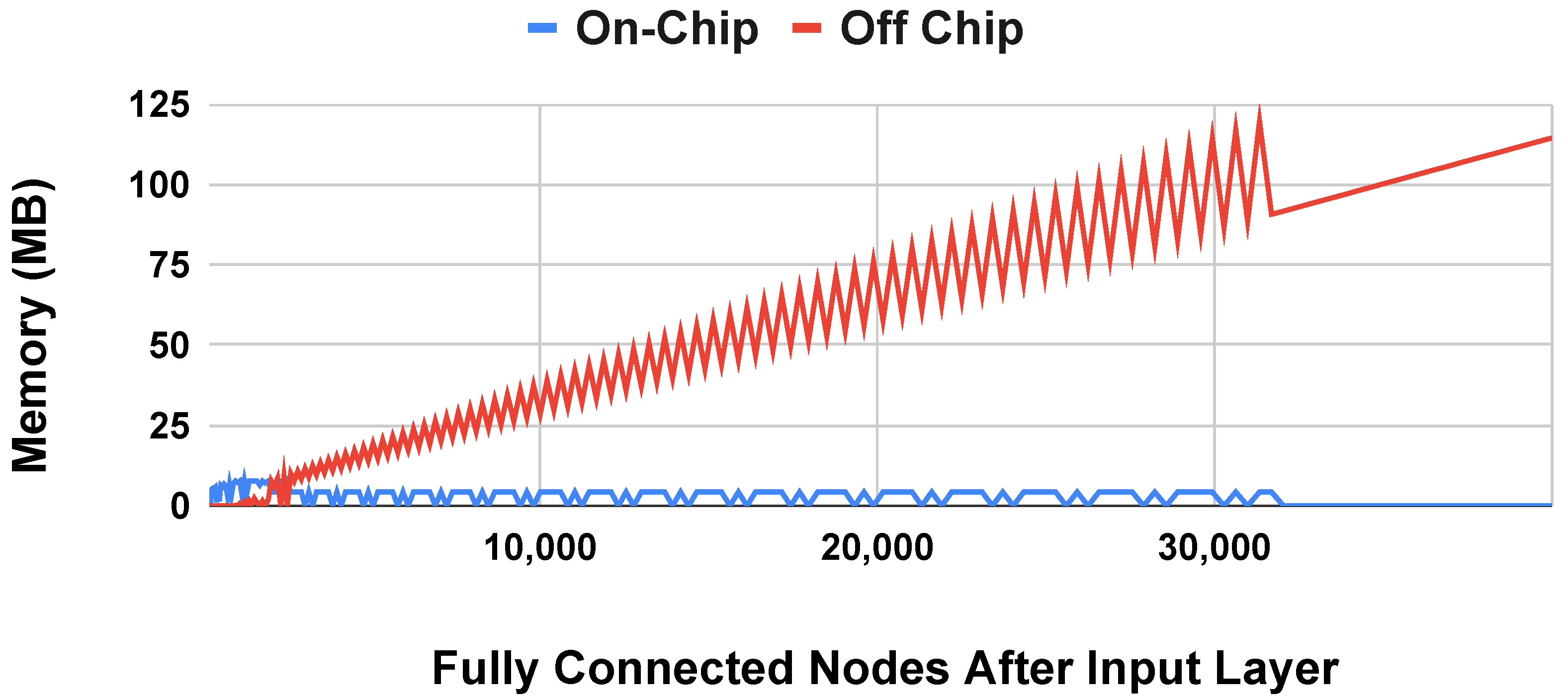
4.3.3. Off-Chip Memory

As previously observed for fully connected, feed-forward neural networks [66], the runtime performance of convolutional neural networks is also affected by the percentage of parameters stored off-chip. Figure 17 shows the TPU runtime performance per inference compared to the percentage of off-chip memory used to store model parameters. We perform this experiment on the models generated from the baseline MobileNet CNN model with scaled filter sizes to increase the width of the model. As the width of the model increases, so does the amount of memory required for parameters, and therefore the amount of off-chip memory used to store parameters also increases. Compared to the results demonstrated in prior work on feed-forward neural networks, CNN runtime scales linearly, instead of in a stepwise manner, due to the increased amount of computation required for CNNs that hides the memory cost of storing parameters off chip.

5. Discussion

Based on our experimental observations in Section 4, we offer the following actionable suggestions for crafting machine learning models tailored to edge devices.

5.1. Prefer Single-Core for Long Term Energy Efficiency but Multi-Core for Energy Efficiency Per Inference

On the baseline CNNs, using a 4-core CPU provided a runtime performance and energy efficiency advantage compared to the 1-core CPU. However, the increase in energy used per inference outweighed the decrease in runtime. Therefore, if inferences will be run continuously in an edge environment, a 1-core CPU will be more energy efficient over time. For bursts of inferences, the 4-core CPU should provide better energy efficiency due to the decrease in runtime.

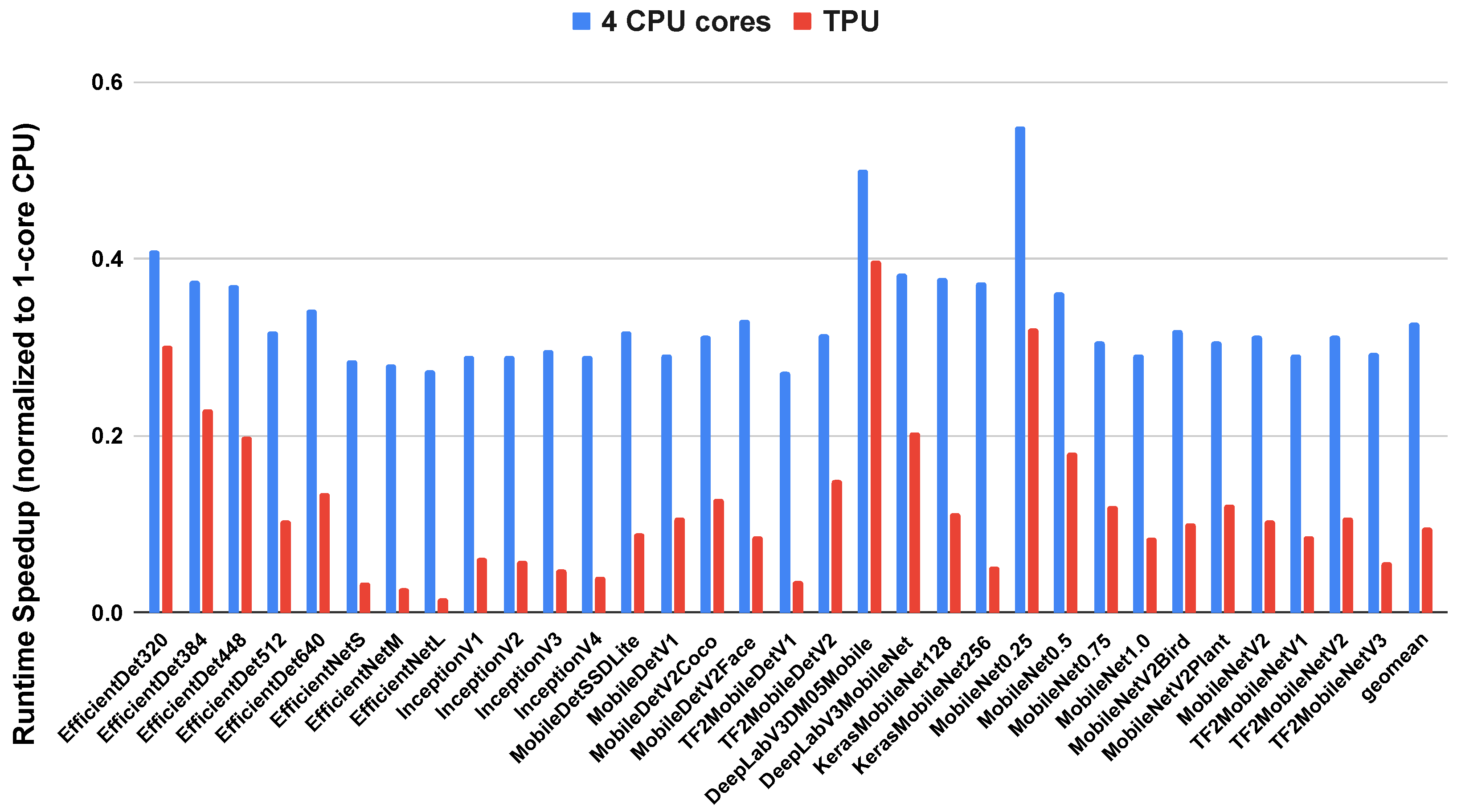
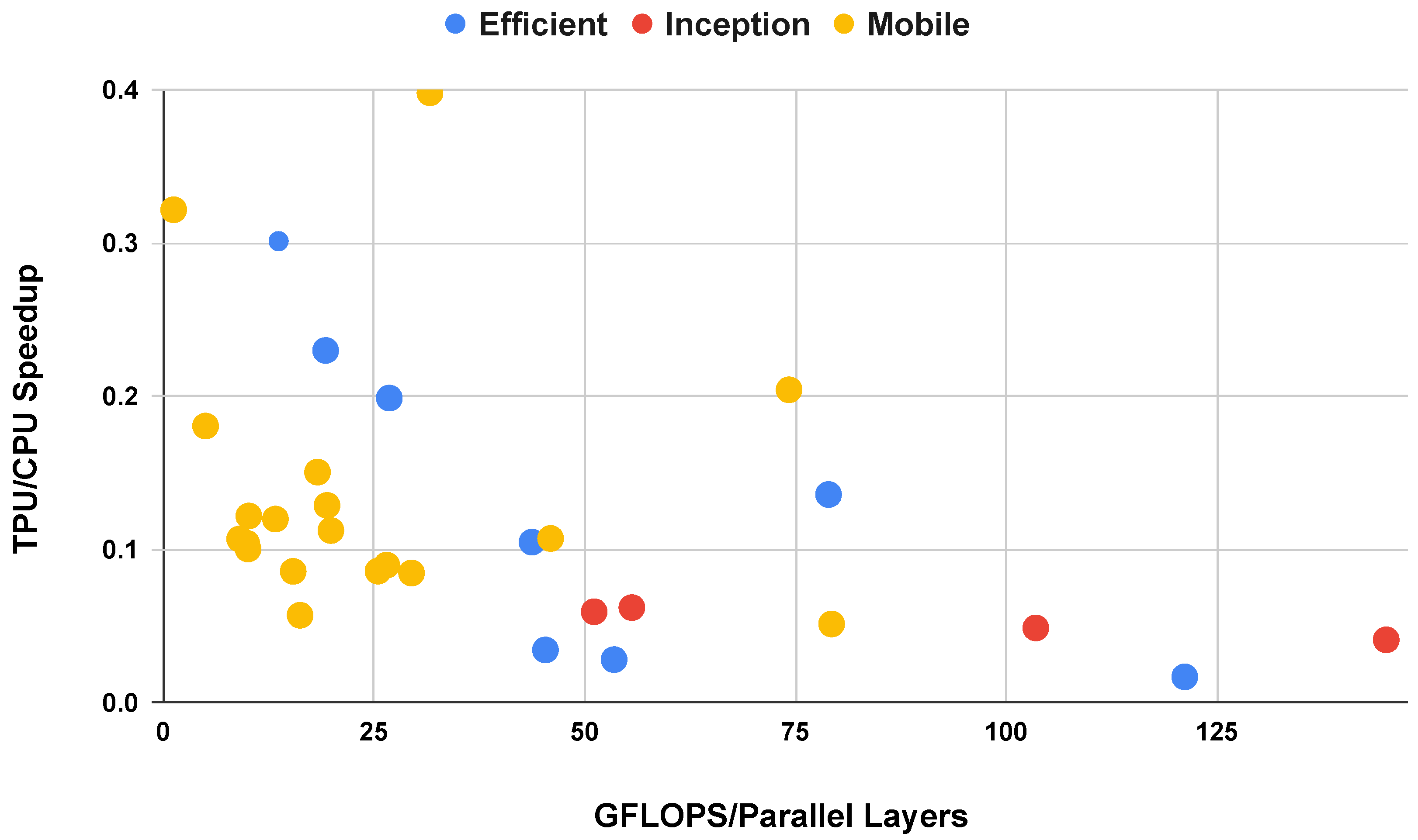
5.2. Prefer a TPU for Convolutional Neural Networks

For all of the convolutional neural networks evaluated in this paper, the TPU outperformed both the single core and 4-core CPU in both runtime performance and energy efficiency. As we scaled the CNN models, both in depth and in width, the TPU continued to consistently outperform the CPU. The only case in which the CPU outperformed the TPU occurred when we added a large fully connected layer to map one-dimensional inputs to the two-dimensional image input expected by the CNN for transfer learning. This case concurs with our findings on the performance degradation of fully connected neural networks on the TPU as the percentage of off-chip memory usage increases.

5.3. For Edge TPUs, Prefer Model Depth When Possible for Convolutional Networks

Due to the width of convolution operations, there is more parallelism inherent to CNNs, and further increasing the width may overload the hardware’s capacity. Table 2 provides a comparison point to a fully connected network with 240 layers and 810 nodes per layer, and all but the smallest CNNs require more floating-point operations to perform an inference.

To mitigate this challenge, it is advisable to focus on expanding the depth of the network instead. We observe symmetry between increases in the depth of the neural network model and its runtime performance on the edge TPU. By increasing the depth, the network can effectively capture complex hierarchical features [68]. Early convolutional neural networks [69] used as few as five layers, but more recent convolutional neural networks, such as Inception-Resnet at 572 layers [60] and the Residual Attention Network at 452 layers, have become significantly deeper. With more data available to train networks, deeper networks can be well-supported by the edge TPU.

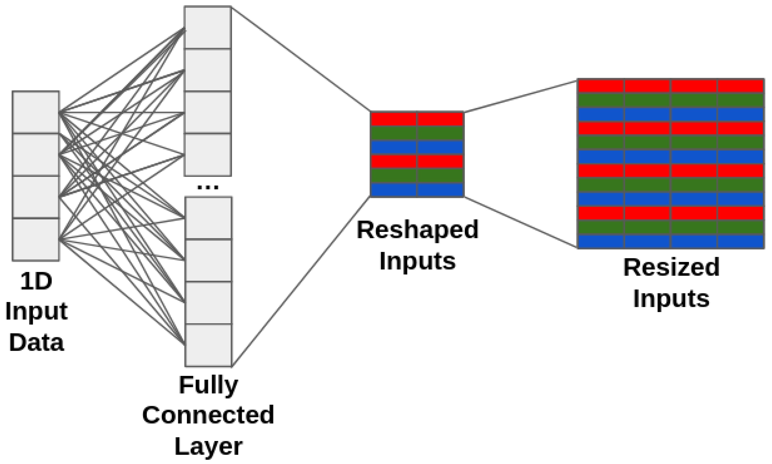
5.4. Avoid Performance Cliffs for Transfer Learning with Fully-Connected Input Layers

As shown in our experiments on transfer learning, the size of a fully connected layer for mapping one-dimensional input data to a two-dimensional image may significantly affect performance. As the number of nodes in the fully connected layer increases, the edgetpu compiler may choose to place all of the model parameters in off-chip memory, leading to asymmetry between the increase in nodes and performance. In our dataset, these performance cliffs were not easy to predict based on the number of nodes in the fully connected layer. However, the performance cliffs occurred infrequently enough that testing the performance of a few fully connected layer sizes should be sufficient to avoid them.

Performance cliffs are common pitfalls for hardware accelerators. NVIDIA provides an occupancy calculator for general-purpose GPU applications (GPGPU) [70] to help application developers choose the correct number of threads and amount of memory to use. We recommend that edge TPU designers provide similar tools to help application developers choose the parameters for their neural networks. However, we note that this is a more complex issue to solve due to the process of developing a neural network model for execution on the edge TPU. The application developer must design the higher level model in a framework like Keras or Tensorflow, then convert the model to Tensorflow Lite, and finally compile the model using the edgetpu compiler. It may be difficult to develop a calculator that accounts for the nuances of this entire process.

5.5. Scale Width at Input Layers to Exploit Parallelism on the Edge TPU

Scaling the width of a convolutional neural network (CNN) at the input layers can be a strategic choice to exploit parallelism and enhance the network’s performance. By increasing the width or the number of channels or filters in the initial convolutional layers, the network gains the ability to capture a broader range of low-level features and patterns from the input data. This enables the CNN to distribute the processing of different features across multiple parallel pathways. Consequently, scaling the width of the network at the input layers can lead to more efficient and effective feature extraction, making it a beneficial strategy for enhancing CNN performance. We observe that the edge TPU effectively exploits the increased parallelism found in the model by increasing its width at the input layers. Therefore, scaling the width at the input layers may increase model accuracy and can be efficiently executed by the edge TPU.

5.6. Limitations

The experiments outlined in this study were performed on the Coral development board. This development board provides features for developing and testing IoT applications, but it is not optimized for deployed applications. For example, the development board runs Mendel Linux, which allows the developer to run programs in a familiar command-line environment. In a deployed IoT application, functionality, like the operating system, that is provided for developer convenience would not be included, leading to performance and energy improvements. We attempted to factor out the energy cost of these convenience features by measuring the resting energy used by the development board, but this may not perfectly model the energy usage of a custom IoT device using a tightly integrated TPU. For custom devices, the methodology presented in this paper can serve as a guide for analyzing the runtime and energy performance of the device on potential network models.

All experiments were run on the Google edge TPU. We leave an evaluation of other accelerators using this methodology to future work. Though the hardware designs that practitioners use to run machine learning models may be slightly different, the methodology for finding the best structure for these models should remain the same, and many of the same takeaways from the discussion will still apply.

We analyze a wide variety of neural network models in this paper, but there are infinitely many ways to structure a neural network. This paper does not evaluate recurrent neural networks such as long short-term memory models, or transformer networks, or other commonly used models. The runtime and energy performance evaluation of additional model structures is left to future work.

We have not evaluated the machine learning algorithm accuracy of these modifications to CNNs. The accuracy of the algorithm is highly dependent on the problem for which machine learning is being applied and on the availability of training data. We leave experimentation on accuracy up to practitioners with a specific problem to solve and hope that the guidance on runtime and energy performance in this paper can assist them in finding an efficient CNN model.

6. Conclusions

In conclusion, this paper has provided an evaluation of the runtime and energy performance of convolutional neural networks (CNNs) when executed on an edge TPU. Our findings underscore the remarkable efficiency gains achieved by leveraging TPUs over traditional CPU architectures. Notably, we have demonstrated that extending the depth of a CNN has a comparatively limited effect on runtime performance in contrast to expanding its width. This insight can guide practitioners in optimizing their model architectures for TPU deployment, emphasizing the potential benefits of deeper networks.

We have analyzed various adjustments to CNNs that might be made by practitioners during the process of applying transfer learning. We find that simply resizing an image input to a different size has little impact on the runtime performance. However, adding a fully connected layer to bridge the gap from a small number of real inputs to the larger number of expected inputs for a CNN may have a significant performance impact on an edge processor.

Furthermore, our investigation has shed light on the role of off-chip memory storage in CNN performance on TPUs. In line with our expectations, the impact of off-chip memory storage appears to be less consequential in the context of convolutional neural networks. This observation highlights the substantial computational requirements inherent to convolution operations, which tend to dominate the overall execution time.

In light of these findings, it is evident that the edge TPU stands as a compelling platform for deploying CNNs, offering not only improved runtime efficiency but also energy savings. As the demand for efficient edge computing solutions continues to rise, our research contributes valuable insights that can aid in the development of optimized models and hardware configurations for real-world applications, especially for practitioners considering an application of transfer learning.

References

1. Jouppi, N.P.; Young, C.; Patil, N.; Patterson, D.; Agrawal, G.; Bajwa, R.; Bates, S.; Bhatia, S.; Boden, N.; Borchers, A.; et al. In-datacenter performance analysis of a tensor processing unit. In Proceedings of the 44th Annual International Symposium on Computer Architecture, Toronto, ON, Canada, 24–28 June 2017; pp. 1–12. [Google Scholar]
2. What Makes TPUs Fine-Tuned for Deep Learning? Available online: https://cloud.google.com/blog/products/ai-machine-learning/what-makes-tpus-fine-tuned-for-deep-learning/ (accessed on 7 May 2022).
3. Xu, D.; Zheng, M.; Jiang, L.; Gu, C.; Tan, R.; Cheng, P. Lightweight and Unobtrusive Data Obfuscation at IoT Edge for Remote Inference. IEEE Internet Things J. 2020, 7, 9540–9551. [Google Scholar] [CrossRef]
4. Dominguez-Morales, J.P.; Duran-Lopez, L.; Gutierrez-Galan, D.; Rios-Navarro, A.; Linares-Barranco, A.; Jimenez-Fernandez, A. Wildlife Monitoring on the Edge: A Performance Evaluation of Embedded Neural Networks on Microcontrollers for Animal Behavior Classification. Sensors 2021, 21, 2975. [Google Scholar] [CrossRef] [PubMed]
5. Kumar, A.; Chakravarthy, S.; Nanthaamornphong, A. Energy-Efficient Deep Neural Networks for EEG Signal Noise Reduction in Next-Generation Green Wireless Networks and Industrial IoT Applications. Symmetry 2023, 15, 2129. [Google Scholar] [CrossRef]
6. Gen7i Transient Recorder and Data Acquisition System. Available online: https://disensors.com/product/gen7i-transient-recorder-and-data-acquisition-system/ (accessed on 20 June 2022).
7. Pouyanfar, S.; Sadiq, S.; Yan, Y.; Tian, H.; Tao, Y.; Reyes, M.P.; Shyu, M.; Chen, S.; Iyengar, S.S. A Survey on Deep Learning: Algorithms, Techniques, and Applications. ACM Comput. Surv. 2019, 51, 92. [Google Scholar] [CrossRef]
8. Alom, M.Z.; Taha, T.M.; Yakopcic, C.; Westberg, S.; Sidike, P.; Nasrin, M.S.; Hasan, M.; Van Essen, B.C.; Awwal, A.A.S.; Asari, V.K. A State-of-the-Art Survey on Deep Learning Theory and Architectures. Electronics 2019, 8, 292. [Google Scholar] [CrossRef]
9. Bebis, G.; Georgiopoulos, M. Feed-forward neural networks. IEEE Potentials 1994, 13, 27–31. [Google Scholar] [CrossRef]
10. Li, Z.; Liu, F.; Yang, W.; Peng, S.; Zhou, J. A Survey of Convolutional Neural Networks: Analysis, Applications, and Prospects. IEEE Trans. Neural Netw. Learn. Syst. 2022, 33, 6999–7019. [Google Scholar] [CrossRef]
11. Zhuang, F.; Qi, Z.; Duan, K.; Xi, D.; Zhu, Y.; Zhu, H.; Xiong, H.; He, Q. A Comprehensive Survey on Transfer Learning. Proc. IEEE 2021, 109, 43–76. [Google Scholar] [CrossRef]
12. You, K.; Kou, Z.; Long, M.; Wang, J. Co-Tuning for Transfer Learning. Adv. Neural Inf. Process. Syst. 2020, 33, 17236–17246. [Google Scholar]
13. Kumar, K.; Khanam, S.; Bhuiyan, M.M.I.; Qazani, M.R.C.; Mondal, S.K.; Asadi, H.; Kabir, H.D.; Khorsavi, A.; Nahavandi, S. SpinalXNet: Transfer Learning with Modified Fully Connected Layer for X-ray Image Classification. In Proceedings of the IEEE International Conference on Recent Advances in Systems Science and Engineering, Shanghai, China, 12–14 December 2021; pp. 1–7. [Google Scholar] [CrossRef]
14. Khosravi, M.R.; Rezaee, K.; Moghimi, M.K.; Wan, S.; Menon, V.G. Crowd Emotion Prediction for Human-Vehicle Interaction Through Modified Transfer Learning and Fuzzy Logic Ranking. IEEE Trans. Intell. Transp. Syst. 2023, 24, 15752–15761. [Google Scholar] [CrossRef]
15. Sharma, A.K.; Nandal, A.; Dhaka, A.; Zhou, L.; Alhudhaif, A.; Alenezi, F.; Polat, K. Brain tumor classification using the modified ResNet50 model based on transfer learning. Biomed. Signal Process. Control 2023, 86, 105299. [Google Scholar] [CrossRef]
16. Kollem, S.; Reddy, K.R.; Prasad, C.R.; Chakraborty, A.; Ajayan, J.; Sreejith, S.; Bhattacharya, S.; Joseph, L.L.; Janapati, R. AlexNet-NDTL: Classification of MRI brain tumor images using modified AlexNet with deep transfer learning and Lipschitz-based data augmentation. Int. J. Imaging Syst. Technol. 2023, 33, 1306–1322. [Google Scholar] [CrossRef]
17. Zheng, Y.; Li, X.; Wang, X.; Zhou, T. Modified Convolutional Neural Network with Transfer Learning for Solar Flare Prediction. J. Korean Astron. Soc. 2019, 52, 217–225. [Google Scholar]
18. Rahman, J.F.; Ahmad, M. Detection of Acute Myeloid Leukemia from Peripheral Blood Smear Images Using Transfer Learning in Modified CNN Architectures. In Proceedings of International Conference on Information and Communication Technology for Development; Studies in Autonomic, Data-driven and Industrial Computing; Springer: Singapore, 2022. [Google Scholar] [CrossRef]
19. Hou, Y.; Ren, H.; Lv, Q.; Wu, L.; Yang, X.; Quan, Y. Radar-Jamming Classification in the Event of Insufficient Samples Using Transfer Learning. Symmetry 2022, 14, 2318. [Google Scholar] [CrossRef]
20. Lanjewar, M.G.; Morajkar, P. Modified transfer learning frameworks to identify potato leaf diseases. Multimed. Tools Appl. 2023. [Google Scholar] [CrossRef]
21. Zhao, X.; Qi, S.; Zhang, B.; Ma, H.; Qian, W.; Yao, Y.; Sun, J. Deep CNN models for pulmonary nodule classification: Model modification, model integration, and transfer learning. J. X-ray Sci. Technol. 2019, 27, 615–629. [Google Scholar] [CrossRef] [PubMed]
22. Sarang, S.; Sheifali, G.; Deepali, G.; Sapna, J.; Amena, M.; Shaker, E.; Kyung-Sup, K. Transfer learning-based modified inception model for the diagnosis of Alzheimer’s disease. Front. Comput. Neurosci. 2022, 16, 1000435. [Google Scholar] [CrossRef]
23. Shin, H.C.; Roth, H.R.; Gao, M.; Lu, L.; Xu, Z.; Nogues, I.; Yao, J.; Mollura, D.; Summers, R.M. Deep Convolutional Neural Networks for Computer-Aided Detection: CNN Architectures, Dataset Characteristics and Transfer Learning. IEEE Trans. Med Imaging 2016, 35, 1285–1298. [Google Scholar] [CrossRef]
24. Wang, X.; Li, J.; Tao, J.; Wu, L.; Mou, C.; Bai, W.; Zheng, X.; Zhu, Z.; Deng, Z. A Recognition Method of Ancient Architectures Based on the Improved Inception V3 Model. Symmetry 2022, 14, 2679. [Google Scholar] [CrossRef]
25. Wang, J.; Chen, Q.; Shi, C. Research on Spider Recognition Technology Based on Transfer Learning and Attention Mechanism. Symmetry 2023, 15, 1727. [Google Scholar] [CrossRef]
26. Edge TPU Performance Benchmarks. Available online: https://coral.ai/docs/edgetpu/benchmarks/ (accessed on 8 May 2022).
27. Kim, B.; Lee, S.; Trivedi, A.R.; Song, W.J. Energy-Efficient Acceleration of Deep Neural Networks on Realtime-Constrained Embedded Edge Devices. IEEE Access 2020, 8, 216259–216270. [Google Scholar] [CrossRef]
28. Yazdanbakshsh, A.; Seshadri, K.; Akin, B.; Laudon, J.; Narayanaswami, R. An Evaluation of Edge TPU Accelerators for Convolutional Neural Networks. arXiv 2020, arXiv:2102.10423. Available online: https://arxiv.org/abs/2102.10423 (accessed on 1 September 2023).
29. Baller, S.P.; Jindal, A.; Chadha, M.; Gerndt, M. DeepEdgeBench: Benchmarking Deep Neural Networks on Edge Devices. In Proceedings of the 2021 IEEE International Conference on Cloud Engineering, San Francisco, CA, USA, 4–8 October 2021; pp. 20–30. [Google Scholar]
30. Jetson Modules. Available online: https://developer.nvidia.com/embedded/jetson-modules (accessed on 27 November 2023).
31. Intel Movidius Vision Processing Units (VPUs). Available online: https://www.intel.com/content/www/us/en/products/details/processors/movidius-vpu.html (accessed on 27 November 2023).
32. AI on Snapdragon Compute Platforms. Available online: https://www.qualcomm.com/products/mobile/snapdragon/pcs-and-tablets/features/computeai (accessed on 27 November 2023).
33. Biglari, A.; Tang, W. A Review of Embedded Machine Learning Based on Hardware, Application, and Sensing Scheme. Sensors 2023, 23, 2131. [Google Scholar] [CrossRef] [PubMed]
34. Ni, Y.; Kim, Y.; Rosing, T.; Imani, M. Online Performance and Power Prediction for Edge TPU via Comprehensive Characterization. In Proceedings of the Design, Automation & Test in Europe Conference & Exhibition, Antwerp, Belgium, 14–23 March 2022; pp. 612–615. [Google Scholar] [CrossRef]
35. Jo, J.; Jeong, S.; Kang, P. Benchmarking GPU-Accelerated Edge Devices. In Proceedings of the IEEE International Conference on Big Data and Smart Computing, Busan, Republic of Korea, 19–22 February 2020; pp. 117–120. [Google Scholar] [CrossRef]
36. Holly, S.; Wendt, A.; Lechner, M. Profiling Energy Consumption of Deep Neural Networks on NVIDIA Jetson Nano. In Proceedings of the 11th International Green and Sustainable Computing Workshops, Pullman, WA, USA, 19–22 October 2020; pp. 1–6. [Google Scholar] [CrossRef]
37. Sun, H.; Qu, Y.; Wang, W.; Dong, C.; Zhang, L.; Wu, Q. An Experimental Study of DNN Operator-Level Performance on Edge Devices. In Proceedings of the IEEE International Conference on Smart Internet of Things, Xining, China, 25–27 August 2023; pp. 131–138. [Google Scholar] [CrossRef]
38. Hosseininoorbin, S.; Layeghy, S.; Sarhan, M.; Jurdak, R.; Portmann, M. Exploring edge TPU for network intrusion detection in IoT. J. Parallel Distrib. Comput. 2023, 179, 104712. [Google Scholar] [CrossRef]
39. Liu, H.; Wang, H. Real-Time Anomaly Detection of Network Traffic Based on CNN. Symmetry 2023, 15, 1205. [Google Scholar] [CrossRef]
40. Hosseininoorbin, S.; Layeghy, S.; Kusy, B.; Jurdak, R.; Portmann, M. Exploring Edge TPU for deep feed-forward neural networks. Internet Things 2023, 22, 100749. [Google Scholar] [CrossRef]
41. Asyraaf Jainuddin, A.; Hou, Y.; Baharuddin, M.; Yussof, S. Performance Analysis of Deep Neural Networks for Object Classification with Edge TPU. In Proceedings of the 8th International Conference on Information Technology and Multimedia, Selangor, Malaysia, 24–26 August 2020; pp. 323–328. [Google Scholar] [CrossRef]
42. Assunção, E.; Gaspar, P.D.; Alibabaei, K.; Simões, M.P.; Proença, H.; Soares, V.N.G.J.; Caldeira, J.M.L.P. Real-Time Image Detection for Edge Devices: A Peach Fruit Detection Application. Future Internet 2022, 14, 323. [Google Scholar] [CrossRef]
43. Morales-García, J.; Bueno-Crespo, A.; Martínez-España, R.; Posadas, J.L.; Manzoni, P.; Cecilia, J.M. Evaluation of low-power devices for smart greenhouse development. J. Supercomput. 2023, 79, 10277–10299. [Google Scholar] [CrossRef]
44. Hou, X.; Guan, Y.; Han, T.; Zhang, N. DistrEdge: Speeding up Convolutional Neural Network Inference on Distributed Edge Devices. In Proceedings of the IEEE International Parallel and Distributed Processing Symposium, Lyon, France, 30 May–3 June 2022; pp. 1097–1107. [Google Scholar] [CrossRef]
45. Nukavarapu, S.; Ayyat, M.; Nadeem, T. iBranchy: An Accelerated Edge Inference Platform for loT Devices. In Proceedings of the IEEE/ACM Symposium on Edge Computing, San Jose, CA, USA, 14–17 December 2021; pp. 392–396. [Google Scholar]
46. Jiang, B.; Cheng, X.; Tang, S.; Ma, X.; Gu, Z.; Fu, S.; Yang, Q.; Liu, M. MLCNN: Cross-Layer Cooperative Optimization and Accelerator Architecture for Speeding Up Deep Learning Applications. In Proceedings of the 2022 IEEE International Parallel and Distributed Processing Symposium, Lyon, France, 30 May–3 June 2022; pp. 1184–1194. [Google Scholar]
47. Guo, J.; Teodorescu, R.; Agrawal, G. Fused DSConv: Optimizing Sparse CNN Inference for Execution on Edge Devices. In Proceedings of the IEEE/ACM 21st International Symposium on Cluster, Cloud and Internet Computing, Melbourne, Australia, 10–13 May 2021; pp. 545–554. [Google Scholar]
48. Arish, S.; Sinha, S.; Smitha, K.G. Optimization of Convolutional Neural Networks on Resource Constrained Devices. In Proceedings of the IEEE Computer Society Annual Symposium on VLSI, Miami, FL, USA, 15–17 July 2019; pp. 19–24. [Google Scholar]
49. Yang, L.; Zheng, C.; Shen, X.; Xie, G. OfpCNN: On-Demand Fine-Grained Partitioning for CNN Inference Acceleration in Heterogeneous Devices. IEEE Trans. Parallel Distrib. Syst. 2023, 34, 3090–3103. [Google Scholar] [CrossRef]
50. Belson, B.; Philippa, B. Speeding up Machine Learning Inference on Edge Devices by Improving Memory Access Patterns using Coroutines. In Proceedings of the IEEE 25th International Conference on Computational Science and Engineering, Wuhan, China, 9–11 December 2022; pp. 9–16. [Google Scholar] [CrossRef]
51. Nasrin, S.; Shylendra, A.; Darabi, N.; Tulabandhula, T.; Gomes, W.; Chakrabarty, A.; Trivedi, A.R. ENOS: Energy-Aware Network Operator Search in Deep Neural Networks. IEEE Access 2022, 10, 81447–81457. [Google Scholar] [CrossRef]
52. Chen, C.; Guo, W.; Wang, Z.; Yang, Y.; Wu, Z.; Li, G. An Energy-Efficient Method for Recurrent Neural Network Inference in Edge Cloud Computing. Symmetry 2022, 14, 2524. [Google Scholar] [CrossRef]
53. Dev Board Datasheet. Available online: https://coral.ai/docs/dev-board/datasheet/ (accessed on 10 May 2022).
54. Arm Cortex-A53 MPCore Processor Technical Reference Manual. Available online: https://developer.arm.com/documentation/ddi0500/latest/ (accessed on 10 May 2022).
55. Trained TensorFlow Models for the Edge TPU. Available online: https://coral.ai/models/ (accessed on 29 January 2022).
56. Tan, M.; Pang, R.; Le, Q. EfficientDet: Scalable and Efficient Object Detection. In Proceedings of the IEEE/CVF Conference on Computer Vision and Pattern Recognition, Seattle, WA, USA, 13–19 June 2020; pp. 10778–10787. [Google Scholar] [CrossRef]
57. Tan, M.; Le, Q. EfficientNet: Rethinking Model Scaling for Convolutional Neural Networks. In Proceedings of the 36th Internation Conference on Machine Learning, PMLR 97, Long Beach, CA, USA, 9–15 June 2019. [Google Scholar]
58. Szegedy, C.; Liu, W.; Jia, Y.; Sermanet, P.; Reed, S.; Anguelov, D.; Erhan, D. Going deeper with convolutions. In Proceedings of the IEEE Conference on Computer Vision and Pattern Recognition, Boston, MA, USA, 7–12 June 2015; pp. 1–9. [Google Scholar] [CrossRef]
59. Szegedy, C.; Vanhoucke, V.; Ioffe, S.; Shlens, J.; Wojna, Z. Rethinking the Inception Architecture for Computer Vision. In Proceedings of the IEEE Conference on Computer Vision and Pattern Recognition, Las Vegas, NV, USA, 27–30 June 2016; pp. 2818–2826. [Google Scholar] [CrossRef]
60. Szegedy, C.; Ioffe, S.; Vanhoucke, V.; Alemi, A. Inception-v4, inception-ResNet and the impact of residual connections on learning. In Proceedings of the Thirty-First AAAI Conference on Artificial Intelligence, San Francisco, CA, USA, 4–9 February 2017; pp. 4278–4284. [Google Scholar]
61. Sandler, M.; Howard, A.; Zhu, M.; Zhmoginov, A.; Chen, L. Mobilenetv2: Inverted residuals and linear bottlenecks. In Proceedings of the IEEE Conference on Computer Vision and Pattern Recognition, Salt Lake City, UT, USA, 18–22 June 2018; pp. 4510–4520. [Google Scholar]
62. Howard, A.; Zhu, M.; Chen, B.; Kalenichenko, D.; Wang, W.; Weyand, T.; Adam, H. MobileNets: Efficient Convolutional Neural Networks for Mobile Vision Applications. arXiv 2017, arXiv:1704.04861. Available online: http://arxiv.org/abs/1704.04861 (accessed on 1 September 2023).
63. Tensorflow 2 Detection Model Zoo. Available online: https://github.com/tensorflow/models/blob/master/research/object_detection/g3doc/tf2_detection_zoo.md (accessed on 28 September 2023).
64. Chen, L.; Zhu, Y.; Papandreou, G.; Schroff, F.; Adam, H. Encoder-Decoder with Atrous Separable Convolution for Semantic Image Segmentation. arXiv 2018, arXiv:1802.02611. Available online: https://arxiv.org/abs/1802.02611 (accessed on 28 September 2023).
65. MobileNet, MobileNetV2, and MobileNetV3. Available online: https://keras.io/api/applications/mobilenet/ (accessed on 28 September 2023).
66. DeLozier, C.; Rooney, F.; Jung, J.; Blanco, J.A.; Rakvic, R.; Shey, J. A Performance Analysis of Deep Neural Network Models on an Edge Tensor Processing Unit. In Proceedings of the International Conference on Electrical, Computer and Energy Technologies, Prague, Czech Republic, 20–22 July 2022; pp. 1–6. [Google Scholar] [CrossRef]
67. Cloud TPU Performance Guide. Available online: https://cloud.google.com/tpu/docs/performance-guide (accessed on 1 September 2023).
68. Charniak, E. Introduction to Deep Learning, 1st ed.; The MIT Press: Cambridge, MA, USA, 2019; pp. 1–192. [Google Scholar]
69. LeCun, Y.; Bengio, Y. Convolutional networks for images, speech, and time series. In The Handbook of Brain Theory and Neural Networks, 1st ed.; The MIT Press: Cambridge, MA, USA, 1998; pp. 255–258. [Google Scholar]
70. Nsight Compute Occupancy Calculator. Available online: https://docs.nvidia.com/nsight-compute/NsightCompute/index.html#occupancy-calculator (accessed on 9 June 2023).
Figure 1. Experimental setup with (counterclockwise from top right to bottom right) a 5 volt, 1 amp power supply connected to the development board’s fan, a 5 volt, 3 amp power supply connected to the development board, a data recorder, the Coral development board, and a laptop for running commands on the development board.
Symmetry 16 00091 g001
Figure 2. Sample power traces for the CPU and TPU on the MobileNet1.0 CNN model.
Symmetry 16 00091 g002
Figure 3. Main subgraphs for EfficientNetS, InceptionV1, and MobileNet1.0.
Symmetry 16 00091 g003
Figure 4. Structure of the main subgraph for InceptionV4. The numbers indicate which layers were added expansions to subgraphs for our transfer learning experiments.
Symmetry 16 00091 g004
Figure 5. Runtime performance (normalized by dividing runtime by the runtime of the 1-core CPU baseline to obtain speedup) of convolutional neural networks on the edge CPU with 1 and 4 cores and on the TPU.
Symmetry 16 00091 g005
Figure 6. Energy per inference (normalized by dividing energy used by the energy used of the 1-core CPU baseline) of convolutional neural networks on the edge CPU with 1 and 4 cores and on the TPU.
Symmetry 16 00091 g006
Figure 7. TPU runtime speedup (TPU runtime divided by CPU runtime, lower is better) compared to floating-point operations per parallel layer. Models are grouped by the base models of EfficientNet, MobileNet, and Inception.
Symmetry 16 00091 g007
Figure 8. Performance impact of varying image input size to CNNs.
Symmetry 16 00091 g008
Figure 9. Adding a fully connected layer to map 1D input data to a 2D CNN. Red, green, and blue cells represent the color format of an image input to a CNN.
Symmetry 16 00091 g009
Figure 10. On-chip and off-chip memory used for adding a fully connected layer to expand 1D inputs to a 2D image.
Symmetry 16 00091 g010
Figure 11. TPU speedup on generated deep CNN models with repeated subgraphs.
Symmetry 16 00091 g011
Figure 12. TPU energy efficiency per inference on generated deep CNN models with repeated subgraphs.
Symmetry 16 00091 g012
Figure 13. TPU runtime performance speedup over CPU on models widened by scaling up input size.
Symmetry 16 00091 g013
Figure 14. CPU and TPU runtime performance on models widened by scaling up output size.
Symmetry 16 00091 g014
Figure 15. CPU and TPU runtime performance on models widened by scaling up input and output size.
Symmetry 16 00091 g015
Figure 16. CPU and TPU runtime prrformance on models widened by adding parallel layers.
Symmetry 16 00091 g016
Figure 17. Execution time for scaled width InceptionV1 in contrast to the proportion of weights stored externally.
Symmetry 16 00091 g017