Systemic Financial Risk Forecasting with Decomposition–Clustering-Ensemble Learning Approach: Evidence from China

Abstract

Establishing a scientifically effective systemic financial risk early warning model is of great significance for prudently mitigating systemic financial risks and enhancing the efficiency of financial supervision. Based on the measurement of systemic financial risk and the network sentiment index of 47 financial institutions, this study adopted the “decomposition–reconstruction–integration” approach, utilizing techniques such as extreme-point symmetric empirical mode decomposition (ESMD), empirical mode decomposition (EMD), variational mode decomposition (VMD), hierarchical clustering, fast independent component analysis (FastICA), attention mechanism, bidirectional long short-term memory neural network (BiLSTM), support vector regression (SVR), and their combination, to construct a systemic financial risk prediction model. The empirical results demonstrate that decomposing and reconstructing relevant indicators before predicting systemic financial risks can enhance prediction accuracy. Among the proposed models, the ESMD-HFastICA-BiLSTM-Attention model exhibits superior performance in systemic financial risk early warning.

1. Introduction

With the continuous advancement of financial integration and the increasingly apparent global financial risks, the stability and sustainable development of financial markets are facing unprecedented challenges. The profound lessons learned from the 2008 financial crisis have led regulatory authorities to recognize the importance of systemic financial risks for financial stability. Countries worldwide are urgently seeking ways to strengthen macroprudential regulatory frameworks and address various vulnerabilities to ensure national financial security. As the world’s second-largest economy, China’s financial market stability directly impacts global economic dynamics and financial system stability [1]. Currently, the Chinese government is facing the dual challenges of addressing the complex economic and financial environment and various unforeseen events, including the Sino–U.S. trade tensions and the COVID-19 pandemic. In such a context, effectively conducting comprehensive and accurate early warnings of China’s systemic financial risk has become an urgent and critical issue to address. Therefore, we aimed to accurately and comprehensively measure China’s systemic financial risk by exploring and proposing effective early warning methods to address various risk challenges that may arise now and in the future. By conducting a comprehensive assessment and early warning of systemic risk in China’s financial system, it can better protect the interests of investors, maintain the stability of global financial markets, and promote sustainable economic development.

Preventing and resolving financial risk has always been a perennial theme in financial work. In the early stages, any situation that threatened the stability of the financial system or undermined public confidence in the financial system was classified as systemic financial risk [2]. However, after the 2008 financial crisis, the academic community defined systemic financial risk as a form of risk contagion and conducted extensive discussions.

Currently, there are two main categories of measurement methods for systemic financial risk. One is the comprehensive index method based on the risk measurement indicator system [3], using the financial stress index as the mainstream method [4]. The other focuses on reflecting the interconnectivity between financial institutions, with metrics mainly including the systemic risk index and marginal expected shortfall [5]. Adrian and Brunnermeier [6] proposed the conditional value at risk (CoVaR) and conditional expected shortfall (MES) to measure the contribution of individual institutions to the overall risk of the financial system. Acharya et al. [7] introduced the marginal expected shortfall (MES) based on expected loss theory to measure the contribution of individual financial institutions to risk. Subsequently, some scholars combined the DCC-GARCH and Copula models, further extending the CoVaR-related indicators [8,9,10,11]. Other researchers considered the impact of leverage and further improved MES, adopting the risk index SRISK, which measures risk in the capital gap [12]. In addition, some scholars explored the contagion of systemic financial risk from a network perspective [13].

A system for providing financial risk warnings is a prerequisite for preventing and controlling systemic financial risks. Currently, in the academic community, models for systemic financial risk warning can be broadly categorized into three types. The first type is early warning models that use binary indicators (1 and 0) to define crisis and non-crisis situations. These models construct regression equations to select warning indicators and assess the likelihood of a crisis outbreak. Common models in this category include the STV cross-sectional regression model, KLR model, etc. Due to drawbacks such as information loss and subjectivity, scholars have sought improvements using the second type of traditional statistical methods. Mainstream methods include autoregressive integrated moving average (ARIMA), generalized autoregressive conditional heteroskedasticity (GARCH), etc. [14,15]. However, these models still face challenges when dealing with nonlinear and non-stationary time series. The third type involves artificial intelligence models. Numerous studies suggest that machine learning and artificial neural networks (ANNs) can effectively enhance the predictive accuracy of traditional statistical methods [16,17]. Subsequently, recurrent neural networks (RNNs) became an important approach in time-series problem research due to their advantages in capturing sequential information [18]. However, RNNs are prone to issues like vanishing or exploding gradients. To address this, scholars introduced gate mechanisms in RNN to control information flow, creating models such as long short-term memory (LSTM) and gated recurrent unit (GRU). These models significantly improve the accuracy of financial time-series warnings [19,20]. At the same time, Shen et al. [21] reported the advantages of convolutional neural networks in stock price prediction. Moreover, scholars have extended these models to bidirectional long short-term memory (BiLSTM) and demonstrated their superiority in forecasting [22,23,24].

Extensive practice has shown that individual artificial intelligence prediction models come with both advantages and disadvantages, making it challenging to achieve optimal predictive performance using a single model. Therefore, most scholars are currently focusing on using ensemble methods to improve the forecasting accuracy of time series. The main approaches can be broadly classified into two categories. The first category involves combining various single models to form a new model. Attention mechanism, which can compute attention probability distributions to extract crucial information and optimize predictive models, is widely used in this context. For example, Ouyang et al. [5] found that attention mechanism significantly improves the predictive accuracy in systemic financial risk warning research. Lu et al. [25] combined convolutional neural network (CNN) and BiLSTM, embedding attention mechanism for stock price prediction, achieving favorable forecasting results.

The second category involves data preprocessing based on the “decomposition–reconstruction–integration” concept. This approach decomposes and reconstructs data into different subsequences, using deep learning models to predict each subsequence separately, finally integrating these parts for an overall analysis [26,27]. Representative decomposition techniques include wavelet decomposition (WD) and empirical mode decomposition (EMD) and its variants, with EMD and its variants being more suitable for the decomposition of nonlinear data [28,29].

Most studies indicate that stock market fluctuations are driven by collective behavior, with investor sentiment playing a particularly significant role in stock market changes [30,31]. This influence not only involves the correlation between investor sentiment and the stock market [32], but also the crucial role of investor sentiment in financial forecasting [33,34]. For example, Gao et al. [35] revealed the significant role of investor sentiment in predicting stock market volatility. As a crucial component of the financial market, stock market volatility can trigger financial risk, and some scholars have demonstrated that investor sentiment has a nonlinear effect in financial risk prediction [36]. Therefore, further exploring the role of investor sentiment in the prediction of systemic financial risk is of significant importance.

By reviewing the above literature, it is evident that individual risk measurement indicators can only assess a certain aspect of systemic financial risk. Moreover, investor sentiment plays a driving role in systemic financial risk, yet few studies have considered investor sentiment as a predictive factor for systemic financial risk. Additionally, obtaining optimal predictive results with a single predictive model is challenging. The widely applied “decomposition–reconstruction–integration” forecasting approach has shown significant improvements in predictive performance. However, there is room for improvement in the methods of “decomposition–reconstruction” [37], and further optimization is needed for deep learning predictive models. Therefore, this paper proposes a systemic financial risk prediction method based on the ESMD-HFastICA-BiLSTM-Attention model. Firstly, four systemic financial risk indicators, CoVaR, ∆CoVaR, MES, and SRISK, are constructed. These indicators are decomposed using extreme-point symmetric empirical mode decomposition (ESMD). Next, a combination of hierarchical clustering and fast independent component analysis (HFastICA) is employed to reconstruct the decomposed data into new subsequences. Finally, investor sentiment measures, such as the network sentiment index and the new subsequences, are used as inputs. The systemic financial risk is predicted through a combination of bidirectional long short-term memory (BiLSTM) and attention mechanism.

This paper’s innovations lie in three aspects. First, the use of the empirical symmetric mode decomposition method effectively overcomes the mode mixing phenomenon encountered in EMD. It does so without the need for additional steps like adding noise, denoising, or smoothing methods, enabling a direct decomposition of the data. Second, the application of hierarchical clustering and fast independent component analysis for data reconstruction results in mutually independent subsequences. This approach avoids subjective reconstruction of subsequences and reduces prediction errors caused by inter-subsequence correlations. Third, the consideration of the network sentiment index is a crucial indicator in forecasting. Additionally, an attention mechanism is incorporated on top of the BiLSTM model, enhancing the focus on important information in the prediction process and improving prediction accuracy.

The remaining structure of this paper is as follows: the second part covers the methodology, the third part deals with indicator calculation and analysis, and the empirical analysis and research conclusion are presented in the fourth and fifth parts, respectively.

2. Methods

2.1. Dynamic Conditional Correlation-Generalized Autoregressive Conditional Heteroskedasticity

We adopted the DCC-GARCH model to calculate the dynamic correlation coefficient between two financial variables. The specific model is as follows:

$$\left\{\begin{array}{l}{H}_t=D_t{R}_t{D}_t\\ R_t=diag{(Q_t)}^{-1/2}{Q}_{t}diag{(Q_t)}^{-1/2}\\ D_t=diag(\sqrt{h_{11,t}},\sqrt{h_{22,t}},\dots ,\sqrt{h_{mm,t}})\\ Q_t=(1-\eta -\omega )\overline{Q}+\omega Q_{t-1}+\eta {\delta }_{i,t-1}{\delta }_{j,t-1}\end{array}\right.,$$

(1)

where $R_t$ represents the matrix of conditional correlation coefficients, $H_t$ represents the matrix of conditional covariance $\sqrt{h_{11,t}}$, $D_t$ represents the diagonal matrix of conditional standard deviations, and the conditional variance $h_{11,t}$ is fitted by a univariate GARCH or TGARCH model. $Q_t=\left[\begin{array}{cc}{q}_{ii,t}& q_{ij,t}\\ q_{ji,t}& q_{jj,t}\end{array}\right]$ is the covariance matrix, $\overline{Q}$ is the matrix of unconditional variances of residuals, $\eta$ is the standardized residual coefficients of lag n, $\omega$ is the coefficients of conditional variances at lag order, all of which are negative and simultaneously satisfy the condition $\eta +\omega <1$. ${\delta }_t$ represents the disturbance term, and j follows a specific distribution.

2.2. Extreme-Point Symmetric Empirical Mode Decomposition

Wang and Li [38] proposed the extreme-point symmetric empirical mode decomposition (ESMD), which addresses the issue of mode mixing in traditional empirical mode decomposition by interpolating the midpoints of line segments connecting local maxima and minima. The ESMD process involves three steps:

Step 1: Identify all local extrema points $E_i(1\le i\le n)$ of the systemic financial risk X (including maxima and minima), connect all adjacent points $E_i$, and label the midpoints of the line segments as $F_i(1\le i\le n-1)$. Then, supplement a left boundary midpoint and a right boundary midpoint by linear interpolation. Utilize n+1 midpoints to construct p interpolation curves $L_1,L_2,\dots ,L_p(p\ge 1)$, and concurrently calculate the average curve $L^{*}=\frac{L_1+L_2+\dots +L_P}{p}$.

Step 2: Repeat Step 1 for $X-L^{*}$. If the iteration reaches the maximum preset value K or satisfies $\left|L^{*}\right|\le \epsilon$ (where $\epsilon$ is the preset error, ${\sigma }_0$ is the standard deviation of data X, and $\epsilon =0.0001{\sigma }_0$ is typically chosen), obtain the first mode $IM{F}_1=m_1$. Repeat the above steps for $X-m_1$ to successively obtain $m_2,m_3,\dots$. Stop when the number of extreme points contained in the residual function $R=X-m_1-m_2-\dots -m_c$ reaches the preset value.

Step 3: Sequentially change the value of K within a pre-defined integer interval $[K_{min},K_{max}]$. Determine $K=K_0$ based on the minimum variance ratio $\sigma /{\sigma }_0$ (where $\sigma$ and ${\sigma }_0$ represent the standard deviations of X − R and X, respectively). Repeat Steps 1 and 2 to obtain the final decomposition result.

2.3. Hierarchical Clustering and Fast Independent Component Analysis

Hierarchical clustering creates a hierarchical tree-like clustering structure by calculating the similarity between different clusters. It is generally divided into agglomerative (bottom–up) and divisive (top–down) approaches. This paper chose the agglomerative hierarchical clustering algorithm. Initially, it assumes each sample is a separate cluster. It then calculates the Manhattan distance between each pair of clusters:

$$d=|x_1^1-x_1^2|+|x_2^1-x_2^2|+\dots +|x_n^1-x_n^2|.$$

(2)

Subsequently, employing the single linkage method, the two sets with the minimum distance are identified, and they are merged into a new set. This process is repeated iteratively until only one set remains. Hierarchical clustering categorizes different intrinsic modes into n classes, forming n random observed signals X. Independent component analysis treats these n random signals as a linear combination of $p(p\le n)$ mutually independent signals s, satisfying:

$$X=AS,$$

(3)

Here X is the known observed signal matrix, S is the unknown independent source vector, and A is the unknown mixing matrix. Then, a separation matrix W is constructed, transforming Equation (3) into $Y=WX=WAS$. Thus, the problem becomes the solution for the separation matrix W. Following the research by Hyvärinen and Oja [39], this paper chose the FastICA method, which maximizes non-Gaussian criteria according to $W^{T}X$ solving the separation matrix W. It constructs the optimization problem of maximizing negative entropy as follows:

$$f_g(W^{T}X)={(E[g(W^{T}X)]-E[g(m)])}^2$$

(4)

where g is a nonlinear function satisfying $g(y)=tanh(by)$, y is a subvector in signal Y, b = 1, $f_g(W^{T}X)$ is negative entropy, $E[\cdot ]$ represents the mean function, and m is a Gaussian random variable after centering and whitening. According to the Kuhn–Tucker conditions, with the constraint $E[{(W^{T}X)}^2]=||W|{|}^2=1$, given $g^{\prime }(\cdot )$ as the derivative of $g(\cdot )$, $W_0$ as the optimized value of W, and $\gamma$ as a constant, the final optimal value is expressed as:

$$\left\{\begin{array}{l}E[X{g}^{\prime }(W^{T}X)]-\gamma W=0\\ \gamma =E[W_0^{T}X{g}^{\prime }(W_0^{T}X)]\end{array}\right..$$

(5)

2.4. Bidirectional Long Short-Term Memory

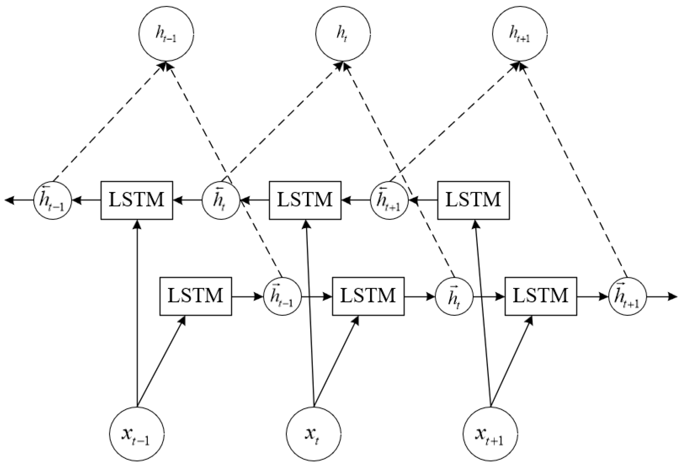
The BiLSTM constructed in this paper consists of two independent LSTMs, namely the forward LSTM and the backward LSTM. Simultaneously considering information from past and future sequences, the final learning result is obtained by combining the forward input sequence and the reverse input sequence with certain weights. The specific model structure is illustrated in Figure 1. To be specific, if $x_{t-1}$, $x_t$ and $x_{t+1}$ are input variables, after going through the forward LSTM, we obtain hidden vectors ${\overrightarrow{h}}_{t-1}$, ${\overrightarrow{h}}_t$ and ${\overrightarrow{h}}_{t+1}$. At the same time, the same input sequences undergo the backward LSTM, yielding hidden vectors ${\overleftarrow{h}}_{t-1}$, ${\overleftarrow{h}}_t$ and ${\overleftarrow{h}}_{t+1}$. Further, concatenating the forward hidden vectors with the backward hidden vectors results in the output of the BiLSTM, represented by $h_{t-1}$, $h_t$ and $h_{t+1}$.

The LSTM cell unit depicted in Figure 1 is primarily composed of a forget gate, an input gate, and an output gate. The forget gate regulates the extent of information to be discarded, while the input and output gates are responsible for receiving and outputting parameters. The specific operational principles are outlined below.

The formula for the forget gate is $f_t=\sigma (W_f\cdot (h_{t-1},x_t)+b_f)$, where $h_{t-1}$ denotes the output at time t−1, $x_t$ is the input to the current layer at time t, $W_f$ is the weights of various variables, and $b_f$ is the bias term. The activation function $\sigma$ determines the retention or omission of information. In this context, the sigmoid function is chosen, with the form $\sigma (x)={(1+e^{-x})}^{-1}$, where $f_t$ ranges between 0 and 1.

The formula for the input gate is $C_t=f_t{C}_{t-1}+i_t{\tilde{C}}_t$, where $i_t=\sigma (W_i\cdot (h_{t-1},x_t)+b_i)$ and ranges between 0 and 1, and $C_t$ represents the updated cell state value. $C_{t-1}$ is the cell state value at time t − 1, ${\tilde{C}}_t=tanh(W_c\cdot (h_{t-1},x_t)+b_c)$ represents the information extracted from the input at time t, and tanh is the hyperbolic tangent activation function. Other types of activation functions can be used as well. And the formula for the output gate is $o_t=\sigma (W_o\cdot (h_{t-1},x_t)+b_o)$, where $o_t$ is the output.

Therefore, LSTM can accomplish internal processing of a neuron through three control gates, forming a memory of long-term past data.

2.5. Attention Mechanism

The attention mechanism can simulate the resource allocation mechanism formed by human attention, allocating probabilistic weights to input elements to reduce the interference of irrelevant information and enhance the significance of key information. If $x_t$ represents the input to the BiLSTM, $h_t$ is the output of each hidden layer after learning, $a_t$ is the attention allocation value to the input of the BiLSTM hidden layer in the attention mechanism, and y is the output value of the BiLSTM with the attention mechanism. The calculation formula is:

$$y={\displaystyle \sum _{t=1}^n{a}_t{h}_t}$$

(6)

Here, $a_t=\frac{\exp (e_t)}{{\displaystyle \sum _{i=1}^n{e}_i}}$ and $e_t=v_{t}tan h(w_t{h}_t+b_t)$ represents the energy value determined by the hidden layer state vector $h_t$ at time t in the BiLSTM. And $v_t$ and $w_t$ are the weight coefficient matrices at time t, and $b_t$ is the bias. The activation function is tan h.

2.6. Prediction Framework and Evaluation Metrics

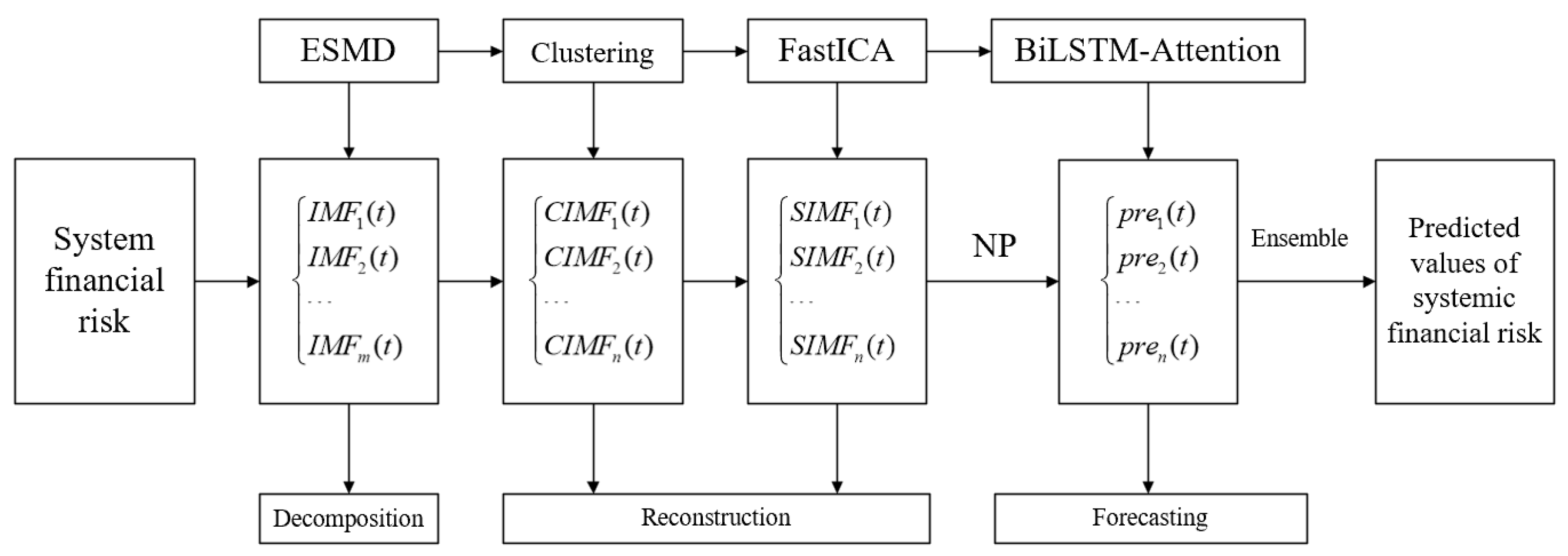
We combined extreme-point symmetric empirical mode decomposition (ESMD), hierarchical clustering and fast independent component analysis (HFastICA), bidirectional long short-term memory (BiLSTM), and attention mechanism, taking into account the crucial indicator of network public opinion. It constructs a novel “decomposition–clustering-ensemble” model for systematic risk prediction. Figure 2 illustrates the structure of the prediction model.

Therefore, the forecasting process of this paper is divided into four steps:

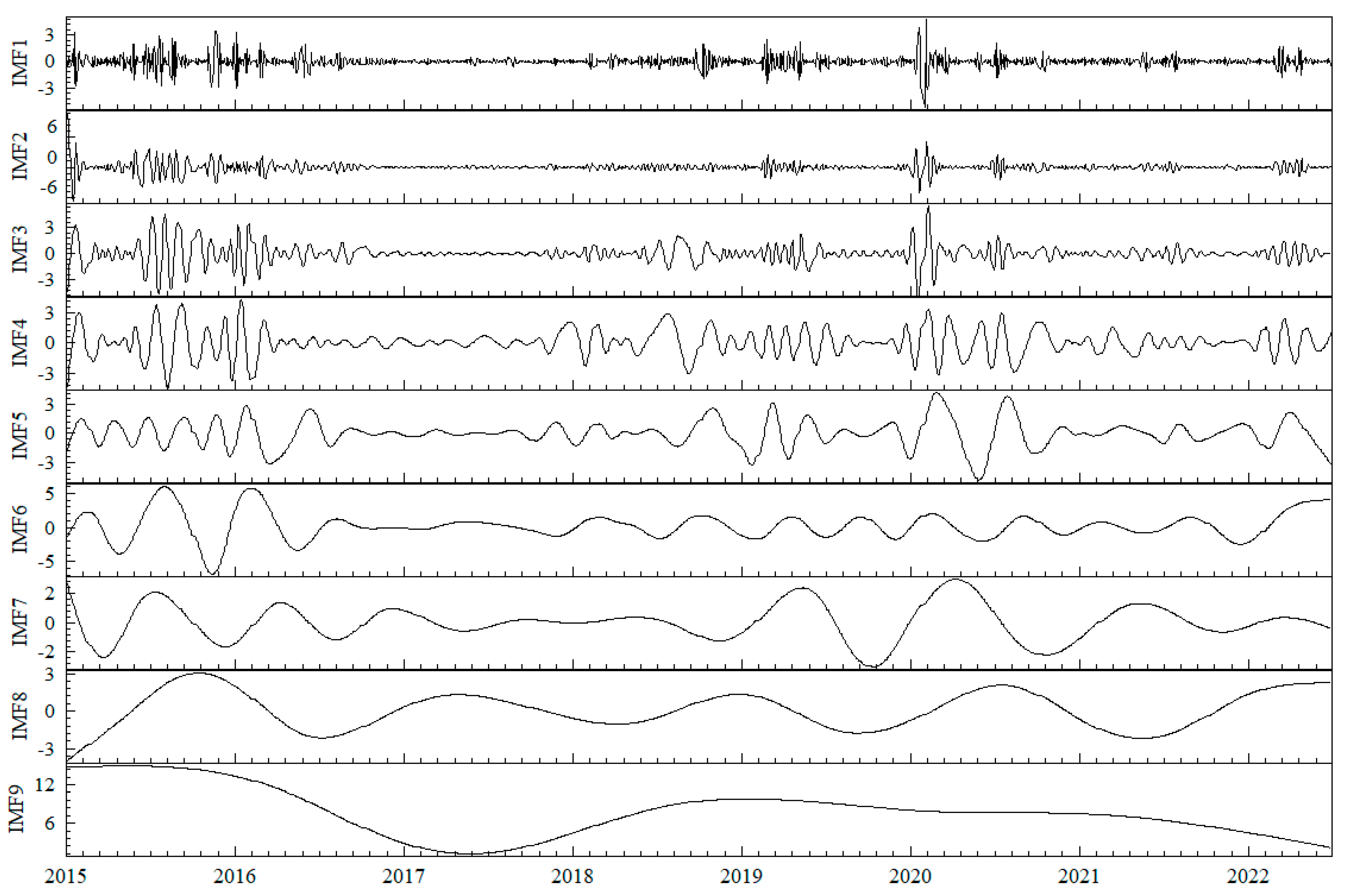
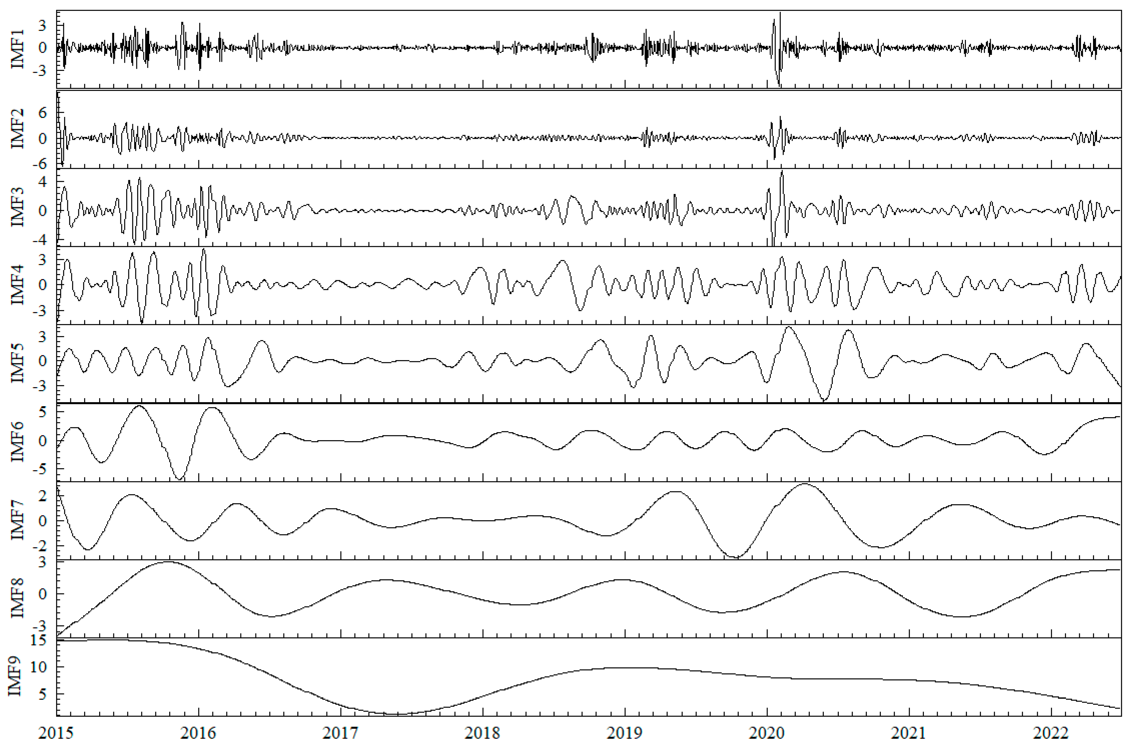
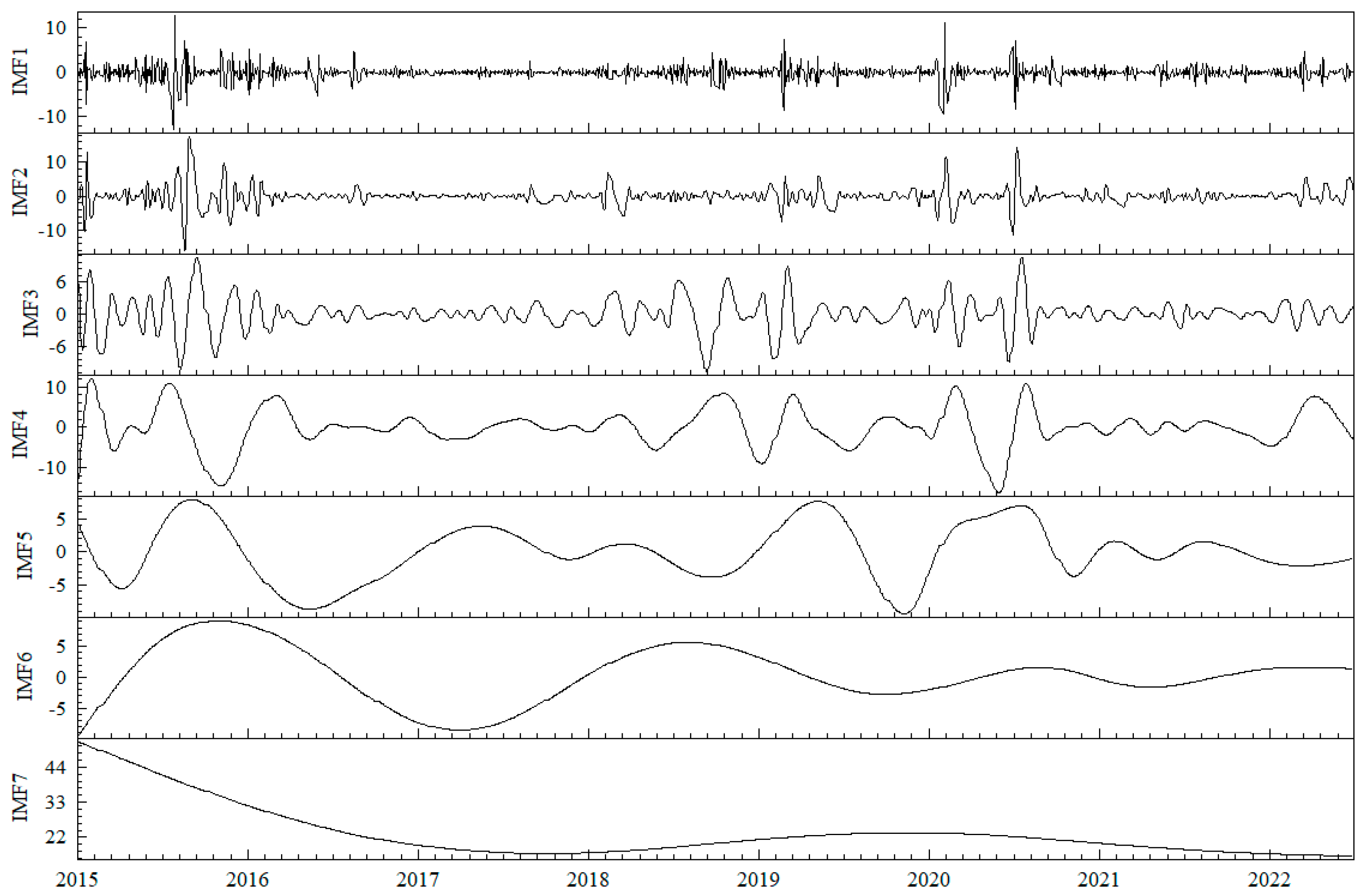
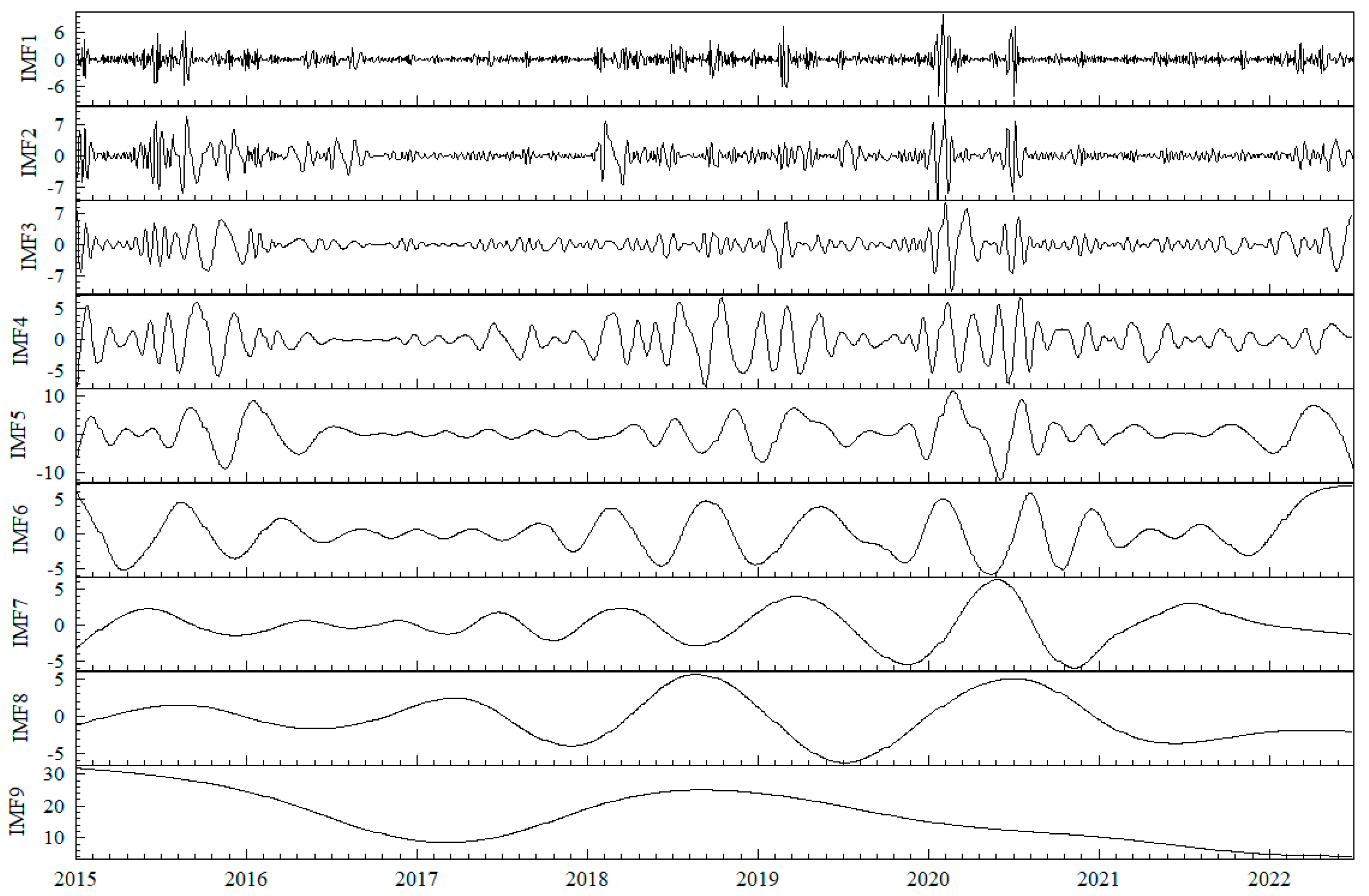
Step 1: Input the forecast indicators of systemic financial risk $x(t)$, and use the ESMD to decompose the observed data into m intrinsic mode functions (IMFs), with $x(t)={\displaystyle \sum _{i=1}^{m}IM{F}_i(t)}$ (the residual sequence is defined as the last mode in this paper).

Step 2: Classify the obtained m mode functions using hierarchical clustering and sum the mode functions of the same category to obtain a new reconstructed sequence, with $x(t)={\displaystyle \sum _{i=1}^{n}CIM{F}_i(t)}$.

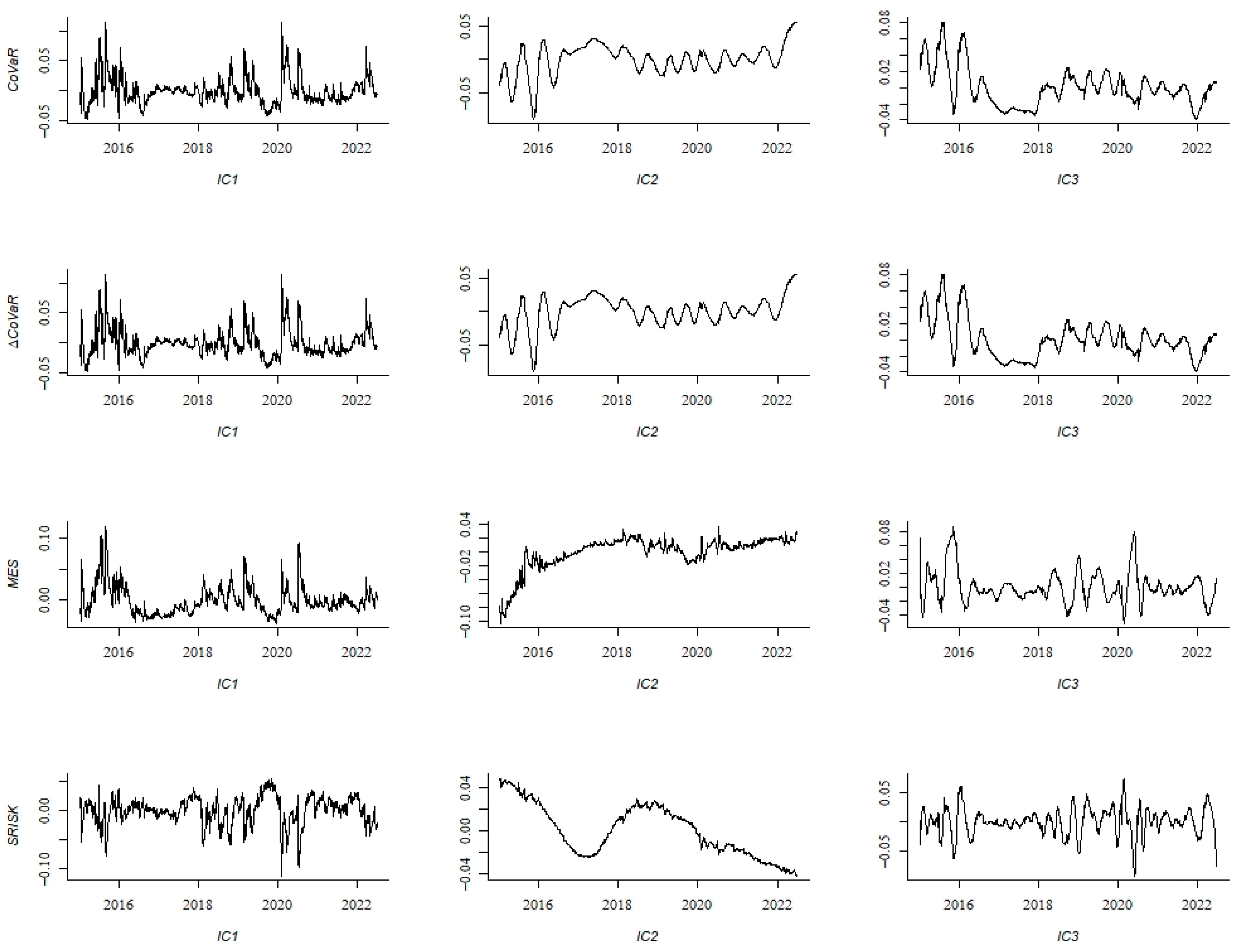
Step 3: Perform FastICA on the reconstructed sequence obtained in Step 2 to obtain mutually independent reconstructed sequences, with $x(t)={\displaystyle \sum _{i=1}^{n}SIM{F}_i(t)}={\displaystyle \sum _{i=1}^n{a}_{i}I{C}_i(t)}$, where $a_i$ is the sum of columns of the mixing matrix and $I{C}_i(t)$ is the estimated signal.

Step 4: Multiply the network public opinion index and the reconstructed sequences from Step 3 by weights as new inputs. Through BiLSTM and attention mechanism, obtain the predicted values of each reconstructed sequence. Integrate all predicted values to obtain the forecast values of systemic financial risk indicators and calculate the evaluation metrics (the specific calculation methods are detailed in

Table 1. Calculation of evaluation metrics.

Evaluation Metrics	Formula
mean absolute error (MAE)	$\frac{1}{N}{\displaystyle \sum _{t=1}^N\left|{\widehat{x}}_t-x_t\right|}$
root mean square error (RMSE)	$\sqrt{\frac{1}{N}{\displaystyle \sum _{t=1}^N{\left({\widehat{x}}_t-x_t\right)}^2}}$
coefficient of determination (R2)	$1-{\displaystyle \sum _{t=1}^N{\left(x_t-{\widehat{x}}_t\right)}^2}/{\displaystyle \sum _{t=1}^N{\left(x_t-{\overline{x}}_t\right)}^2}$
directional prediction statistic (Dstat)	$\frac{1}{N}{\displaystyle \sum _{i=1}^{N}r(t)\times 100\%},r(t)=\left\{\begin{array}{l}1,(x_{t+1}-x_t)({\stackrel{⌢}{x}}_{t+1}-{\stackrel{⌢}{x}}_t)\ge 0\\ 0,(x_{t+1}-x_t)({\stackrel{⌢}{x}}_{t+1}-{\stackrel{⌢}{x}}_t)\le 0\end{array}\right.$

Note: N is the number of data points, $x_t$ represents the actual values, ${\widehat{x}}_t$ represents the predicted values, and ${\overline{x}}_t$ is the mean value.

).

3. Indicator Calculation and Analysis

3.1. Calculation of Systemic Financial Risk Indicators

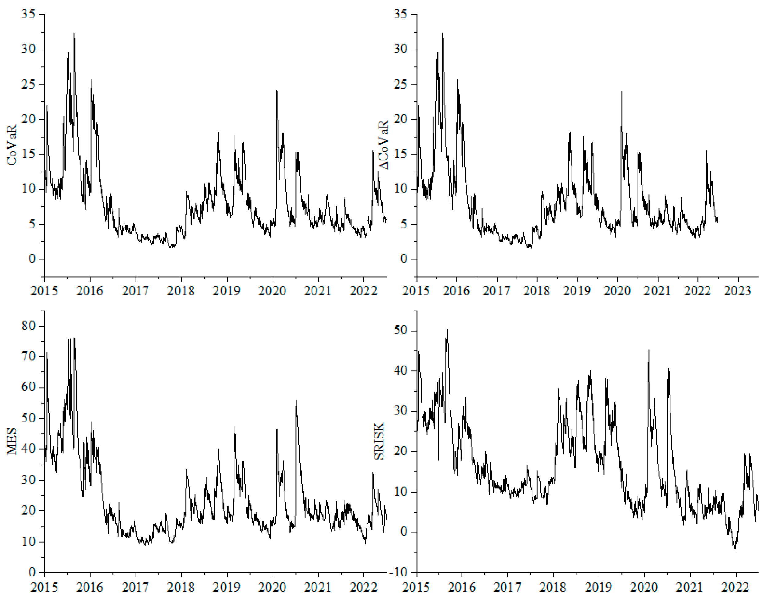
To ensure the universality and representativeness of the research results, we selected all financial institutions listed on the A-share market before 2014 as our research sample. We excluded institutions with missing data and considered the availability of text data from the East Money Stock Bar. Eventually, we identified 47 financial institutions, all of which have a market share exceeding 70% and thus play a dominant role in the financial market. We calculated their daily logarithmic return, and the market index was measured using the daily logarithmic returns of the CSI 300 index. The sample period extended from 2 January 2015 to 30 June 2022, and all data were sourced from CSMAR.

We measured China’s systemic financial risk from various perspectives using conditional value at risk (CoVaR), conditional value at risk difference (∆CoVaR), marginal expected shortfall (MES), and the capital shortfall risk index (SRISK). CoVaR emphasizes the risk spillover of individual financial institutions to others or the entire market. ∆CoVaR reflects the difference between CoVaR when a single institution is in an extreme state and when the system is normal. MES reflects the marginal contribution of individual financial institutions to systemic risk during a significant market return decline. SRISK reflects systemic risk from the expected capital shortfall perspective.

(1) CoVaR Calculation: CoVaR is defined as $\mathrm{Pr}(X^s\le CoVa{R}_q^{s/i}|X^i=Va{R}_q^i)=q$ by Adrian and Brunnermeier [6], representing the risk value level of the financial system at confidence level q when financial institution i experiences a crisis, where $X^s$ represents the financial system’s return. We chose q = 0.05 and used the CSI 300 index logarithmic return to represent the financial system’s return. Equation (1) was used to calculate the dynamic CoVaR value for individual financial institution i.

(2) ∆CoVaR Calculation: setting q = 0.05 and q = 0.5 as extreme and normal states, respectively, we calculated the CoVaR value for individual financial institutions in different states. ∆CoVaR was calculated by computing $\Delta CoVa{R}_{t,0.05}^{s\left|i\right.}=CoVa{R}_{t,0.05}^{s\left|i\right.}-CoVa{R}_{t,0.5}^{s|i}$.

(3) MES Calculation: Acharya et al. [7] defined MES as $ME{S}_{i,t}=E(r_{i,t}|r_{s,t}<q)$, where $r_{s,t}$ is the CSI 300 index logarithmic return and $r_{i,t}$ is the logarithmic return of individual financial institutions. We set q = 0.05 and calculated the dynamic MES using Equation (1).

(4) SRISK Calculation: Based on the MES calculation results, setting k = 0.08, we computed $SRIS{K}_{i,t}=k{D}_{i,t}-(1-k)(1-LRME{S}_{i,t})\ast E_{i,t}$, where the long-term marginal expected loss $LRME{S}_{i,t}=1-exp\left(-18\times ME{S}_{i,t}\right)$, where $D_{i,t}$ and $E_{i,t}$ represent the book value of debt and equity, sourced from CSMAR.

Based on the calculation of systemic financial risk values for individual financial institutions, we computed the weighted average of CoVaR, ∆CoVaR, MES, and SRISK for 47 institutions using market capitalization as weights. These values represent the overall systemic financial risk for China, serving as the basis for subsequent research in this paper. Due to the small scale of these four systemic financial risk indicators, we multiplied all indicators by 1000 for subsequent research. Figure 3 shows the time series of systemic financial risk, indicating similar trends in the four indicators. In the second half of 2015, the abnormal fluctuations in the A-share market significantly impacted the Chinese economy, leading to a drastic fluctuation in systemic financial risk. The sustained high level of risk exacerbated the transmission and diffusion of risks, causing substantial harm to both financial markets and the real economy. This warrants close attention from regulatory authorities and proactive preventive measures. The second significant fluctuation occurred in 2018, driven by the ongoing trade tensions between the U.S. and China, financial reforms domestically, and the release of certain risks into the market, inducing panic. However, due to the proactive response from relevant Chinese authorities, the systemic risk gradually declined to a relatively stable state after the initial rise. The third major fluctuation emerged after 2020, coinciding with the outbreak of the COVID-19 pandemic in China. This event had a significant impact on the Chinese and global economies. Nevertheless, the Chinese government promptly implemented effective epidemic control measures and introduced a series of policies to stabilize the market. This allowed businesses to resume operations quickly, leading to a gradual recovery of the economy after a brief shock.

3.2. Calculation of Network Public Opinion Index

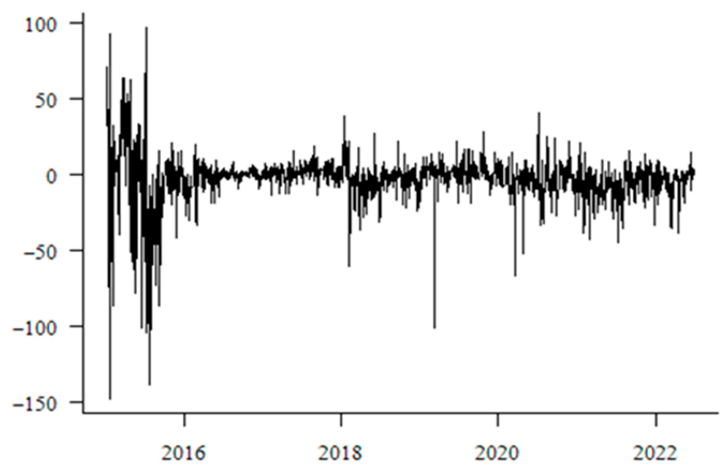
Drawing on the research methodology of Ouyang Zisheng et al. [36], this paper utilized python to crawl comment data for 47 listed companies on East Money’s website from 5 January 2015 to 30 June 2022. The collected data included post titles, click-through rates, reply counts, usernames, posting times, and post content. As stock market forums serve as open platforms for information exchange, containing both emotional expressions of investors facing market changes and a certain amount of irrelevant information, the obtained data underwent thorough cleaning. This process involved removing advertising posts from the scraped information and eliminating duplicate sentences and words.

Following data cleaning, the text data underwent segmentation, a common method for Chinese text segmentation that combines rule-based and statistical approaches. Leveraging python’s Jieba, Dalian University of Technology, Sogou lexicons, as well as specialized sentiment lexicons for the stock market and stock forums, we achieved text segmentation and feature extraction. Additionally, sentiment analysis categorized network sentiment into optimistic, neutral, and pessimistic sentiments. Each comment was analyzed, and the quantities of positive, neutral, and negative vocabulary were calculated. Positive sentiment words were assigned a value of 1, negative sentiment words −1, and neutral sentiment words 0. The sum of these three sentiment categories for each day resulted in the daily network public opinion index (NP), acting as a proxy indicator for investor sentiment, with its trend depicted in Figure 4. Clearly, after 2016, the fluctuation range of the network public opinion index is relatively small, except for occasional times when the variation range is basically within the [−50, 50] interval. However, during the period from 2015 to 2016, the network public opinion index showed extreme volatility. The reason for this is that in 2015, the “stock market crash” caused the Chinese stock market to experience drastic fluctuations of collapse, rebound, and subsequent adjustments, leading to repeated changes in investor sentiment between optimism and panic. Combined with the herd effect and emotion-driven behavior of investors, this resulted in exceptionally violent fluctuations in the network public opinion index during this period.

3.3. Data Description and Interrelationship Analysis

Figure 3 and Figure 4 depict the temporal characteristics of China’s systemic financial risk and network public opinion index. To further understand the distributional properties of the data,

Table 2. Descriptive statistics.

	Number	Min	Max	Mean	St
NP	1822	−147.5925	97.0208	−2.4110	16.1111
CoVaR	1822	1.6425	32.4396	8.0391	5.1847
ΔCoVaR	1822	1.6389	32.4002	8.0249	5.1774
MES	1822	8.7679	76.2122	23.3972	12.3060
SRISK	1822	−4.9172	50.2667	16.4566	10.4247

provides descriptive statistics for both datasets, including the sample size (Number), minimum value (Min), maximum value (Max), mean (Mean), and standard deviation (St). The standard deviation of the network public opinion index is 16.1111, indicating a large variability within the sample period, with a mean of −2.4110, suggesting a prevailing negative sentiment among investors in the Chinese financial system during the sample period. We observe that MES exhibits the greatest fluctuation among the four systemic financial risk indicators, while ∆CoVaR has the smallest standard deviation. The minimum value of SRISK is negative, indicating that the debt of the financial system exceeded its assets during those periods. The distinct statistical characteristics of the four systemic financial risk indicators illustrate their varied perspectives on China’s systemic financial risk.

The interrelationship between network public opinion and systemic financial risk manifests in two aspects. On the one hand, investors, as the mediators influencing systemic financial risk through network public opinion, can gather and interpret information from online sentiment, understand various investors’ expectations for the financial market, engage in information exchange, and share insights. However, such sentiment-laden information can lead investors to make irrational judgments, causing market overfluctuations, investment bubbles, and triggering systemic financial risk. On the other hand, in the era of digital information, the rapid and diverse dissemination of public sentiment information may result in varying qualities of information. Due to limited investor attention, this can lead to the transmission of false or erroneous information, creating an asymmetry of information in the market. Consequently, in situations of rapid market changes, investors might make inaccurate decisions, causing significant market fluctuations and exacerbating systemic financial risk. Therefore, the network public opinion index can serve as a crucial indicator for predicting systemic financial risk.

We employed the generalized forecast error variance decomposition method proposed by Diebold and Yilmaz [40] to construct the spillover matrices between the network public opinion index and systemic financial risk. The interrelationship between the network public opinion index and systemic financial risk was examined, and the rationality of using the network public opinion index as a predictor for systemic financial risk was tested.

Table 3. The information spillover matrix.

	NP	CoVaR	∆CoVaR	MES	SRISK	From
NP	99.92	0.01	0.01	0.02	0.05	0.08
CoVaR	76.48	2.12	2.11	3.45	15.84	97.88
∆CoVaR	76.49	2.12	2.11	3.45	15.83	97.89
MES	27.68	2.01	2.00	12.01	56.29	87.99
SRISK	51.75	0.02	0.02	0.18	48.03	51.97
To	232.39	4.16	4.15	7.10	88.01	67.16

presents the spillover matrices calculated through vector autoregression and variance decomposition, where “To” indicates spillovers, and “From” indicates inward spillovers. Overall, the information spillover of the network public opinion index was as high as 232.39%, while the inward spillover was only 0.08%. This suggests that the impact of network public opinion on the four categories of systemic financial risk is far greater than the impact of systemic risk on network public opinion index. Among them, CoVaR, ∆CoVaR, and SRISK, the three types of systemic financial risk, receive information spillovers mainly from the network public opinion index, accounting for 76.48%, 76.49%, and 51.75%, respectively. The information spillover of the network public opinion index to MES is 27.68%, ranking second in the spillover into MES. Nevertheless, this still indicates the significant role of network public opinion in predicting systemic risk. There are asymmetric information spillovers and spillovers among the four types of systemic financial risk, indicating that these indicators have certain correlations but also differences. Therefore, different dimensions of the systemic financial risk indicators should be considered in predictions.

4. Results

4.1. Decomposition, Clustering, and Reconstruction

Before conducting the prediction of systemic financial risk, this paper preprocessed the systemic financial risk data through decomposition, clustering and reconstruction to fully exploit the data information. To reconstruct the data, the relevant steps of ESMD were applied to decompose CoVaR, ∆CoVaR, MES, and SRISK. Figure 5, Figure 6, Figure 7 and Figure 8 depict the decomposition results for the four types of systemic financial risk. CoVaR, ∆CoVaR, MES, and SRISK were decomposed into 9, 9, 7, and 9 intrinsic mode functions (IMFs), respectively. Among these, the frequency of each mode from IMF1 to IMF9 (IMF7) gradually decreased, with IMF1 having the highest frequency and the smallest amplitude, which can be considered as representing random factors. IMF2 to IMF6 (MES is IMF2 to IMF4) exhibited normal frequencies and amplitudes. IMF7 to IMF8 (MES is IMF5 to IMF6) represent low-frequency data, reflecting the long-term changes in systemic financial risk. The last mode (i.e., residual) was smooth and changed slowly, reflecting the overall trend of the systemic financial risk. It reached its highest point in 2015, experienced a significant decline thereafter, rose again after 2018, and then gradually decreased with slight fluctuations in 2022.

If the decomposed data are directly used for prediction, this not only increases the prediction time but may also lead to inaccuracies in the prediction of individual modes due to the correlation between modes. Therefore, before applying deep learning for prediction, this study reconstructed the decomposed systemic financial risk data from ESMD. Both hierarchical clustering and FastICA were employed for data reconstruction, referred to as HFastICA. Hierarchical clustering offers flexibility and does not require specification of the number of clusters, while FastICA further extracts mutually independent information sequences to capture the basic structure of the prediction data.

Table 4. Inherent modal categories of systemic financial risk.

	IMF1	IMF2	IMF3	IMF4	IMF5	IMF6	IMF7	IMF8	IMF9
CoVaR	1	1	1	1	1	2	1	1	3
∆CoVaR	1	1	1	1	1	2	1	1	3
MES	1	1	1	2	1	1	3	—	—
SRISK	1	1	1	1	2	1	1	1	3

presents the hierarchical clustering results for CoVaR, ∆CoVaR, MES, and SRISK, categorizing the modes into different clusters. These results were computed using Equations (2), (4) and (5). The modal functions within the same cluster of each systemic financial risk type were summed to obtain the new sub-series CIMF, resulting in three reconstructed sub-series (CIMF1, CIMF2, and CIMF3).

Next, the FastICA method was used to extract the independent signals from the CIMF subseries. By solving the optimization problem of maximizing negative entropy, the estimated values of the mixing matrix were obtained. Figure 9 shows the three independent components (IC) extracted for various systemic financial risk indicators. The change trends of the independent components of CoVaR and ∆CoVaR are similar, but they differ significantly from those of MES and SRISK. Among them, the change trend of IC1 for CoVaR, ∆CoVaR, and MES was close to the original sequence, while the absolute value of the correlation coefficient between IC1 and the corresponding original sequence for SRISK was similar in trend. They were 0.6943, 0.6942, 0.8583, and 0.6981, respectively. Therefore, IC1 can be regarded as a reflection of systemic financial risk on itself, indicating that historical data has an important role in the fluctuation of systemic financial risk.

Compared to IC2, IC3 has a trend similar to the corresponding original sequence, but it is relatively smooth, with significant changes during important financial shocks. Therefore, IC2 can be interpreted as the impact of other factors on the variation of systemic financial risk, while IC3 can be interpreted as the impact of financial shocks on systemic financial risk. During the “stock market crash” in 2015, the China–US trade friction in 2018, and the COVID-19 pandemic in 2020, IC3 showed varying degrees of changes.

The signals extracted by FastICA need to exhibit independence and non-Gaussian characteristics. This study assessed the independence and non-Gaussian nature of each independent signal using correlation coefficients and normality tests. The results in

Table 5. Independent component test.

		S-W Test	J-B Test	A-D Test	K-S Test	Correlation
CoVaR	IC1	0.9029 ***	1245.5000 ***	50.6260 ***	0.1394 ***	1.0000
	IC2	0.9487 ***	553.0500 ***	21.3150 ***	0.0631 ***	$2.3661\times {10}^{-9}$
	IC3	0.9231 ***	457.6500 ***	34.5910 ***	0.1082 ***	$-4.2929\times {10}^{-9}$
∆CoVaR	IC1	0.9029 ***	1245.5000 ***	50.6260 ***	0.1394 ***	1.0000
	IC2	0.9487 ***	553.0500 ***	21.3150 ***	0.0631 ***	$2.3661\times {10}^{-9}$
	IC3	0.9231 ***	457.6500 ***	34.5910 ***	0.1082 ***	$-4.2929\times {10}^{-9}$
MES	IC1	0.8822 ***	1758.1000 ***	47.5650 ***	0.1116 ***	1.0000
	IC2	0.7832 ***	2780.3000 ***	115.0800 ***	0.1610 ***	$1.8701\times {10}^{-9}$
	IC3	0.9157 ***	768.02000 ***	43.2650 ***	0.1108 ***	$-2.8217\times {10}^{-9}$
SRISK	IC1	0.9625 ***	382.9900 ***	16.5530 ***	0.0779 ***	1.0000
	IC2	0.9572 ***	102.4700 ***	26.2550 ***	0.1068 ***	$-1.6429\times {10}^{-9}$
	IC3	0.9707 ***	222.9600 ***	18.4760 ***	0.1084 ***	$1.4161\times {10}^{-9}$

Note: *** represents significance at the 0.01 levels.

indicate that all ICs do not follow a normal distribution and are statistically significant at the 1% level. Moreover, the correlation coefficients are close to 0, demonstrating that the ICs possess independence and are non-Gaussian.

As the original data satisfies $x(t)={\displaystyle \sum _{i=1}^{n}SIM{F}_i(t)}={\displaystyle \sum _{i=1}^n{a}_{i}I{C}_i(t)}$ after FastICA analysis,

Table 6. Calculation of systematic financial risk SIMF.

Indicator	Component	Calculation
CoVaR	SIMF1	$153.6004\times \mathrm{I}\mathrm{C}1$
	SIMF2	$-39.7747\times \mathrm{I}\mathrm{C}2$
	SIMF3	$154.1919\times \mathrm{I}\mathrm{C}3$
∆CoVaR	SIMF1	$153.3749\times \mathrm{I}\mathrm{C}1$
	SIMF2	$-39.8344\times \mathrm{I}\mathrm{C}2$
	SIMF3	$153.9553\times \mathrm{I}\mathrm{C}3$
MES	SIMF1	$450.7472\times \mathrm{I}\mathrm{C}1$
	SIMF2	$-269.2967\times \mathrm{I}\mathrm{C}2$
	SIMF3	$8.4929\times \mathrm{I}\mathrm{C}3$
SRISK	SIMF1	$-310.5547\times \mathrm{I}\mathrm{C}1$
	SIMF2	$310.7411\times \mathrm{I}\mathrm{C}2$
	SIMF3	$69.9420\times \mathrm{I}\mathrm{C}3$

provides the corresponding weights and the calculated SIMFs. Finally, the SIMFs are used as input for the prediction of systematic financial risk.

4.2. Prediction Results of Systematic Financial Risk

Before using deep learning or machine learning for prediction, it is a common practice to normalize the data. This helps eliminate the interference of feature dimensions on the prediction results and improves the model’s generalization ability. Specifically, data normalization refers to transforming the input and prediction data into a uniform distribution within a specific range, typically [0, 1] or [−1, 1]. For this study, the final prediction data obtained from decomposition and reconstruction are independent components of systemic financial risk (SIMF), and the input data are the network public opinion index. We normalized each SIMF and the network public opinion index, using the Min–Max normalization function in python to transform them to [−1, 1]. Additionally, we split the data into training and testing sets in a 7:3 ratio. Through the grid search method, the following parameter configuration was finally determined: The BiLSTM layer was set with 25 neuron nodes, the number of iterations was set to 100, batch size was set to 16, the output neuron count was 1, and the activation function was chosen as “tanh”. In the attention layer, the activation function was “softmax”.

Since the stock market operates 5 days a week, a forward-looking 5-step prediction was selected. SIMF and the network public opinion index were used as outputs. After passing through the BiLSTM-Attention network, the results were integrated to obtain the predicted values of systemic financial risk. Figure 10 shows the changes in the predicted values and real values of CoVaR, ∆CoVaR, MES, and SRISK from January to June 2022. Among them, the deviation of SRISK is larger than the other three indicators, but overall, the ESMD-HFastICA-BiLSTM-Attention model can predict the changing trend of systemic financial risk well.

The prediction of this paper consists of two parts: data preprocessing and deep learning prediction. In the data preprocessing stage, ESMD decomposition and HFastICA reconstruction were employed. In the deep learning prediction part, BiLSTM and the attention mechanism were selected. Therefore, the effectiveness of the ESMD-HFastICA-BiLSTM-Attention prediction model was explained from these two aspects. First, in the data preprocessing stage the effectiveness was examined from the perspectives of whether the data was reconstructed and different decomposition methods.

Table 7. Predictive results of whether to reconstruct.

		CoVaR	ΔCoVaR	MES	SRISK
Original data	MAE	0.4008	0.4845	1.2883	1.5421
	RMSE	0.7044	0.7315	1.8745	2.0597
	R2	0.9290	0.9231	0.9291	0.9249
	Dstat	0.5321	0.5431	0.6018	0.5890
Decomposition	MAE	0.1118	0.2993	0.6946	1.0232
	RMSE	0.1732	0.4855	1.0997	1.3854
	R2	0.9957	0.9652	0.9756	0.9660
	Dstat	0.9193	0.6220	0.7083	0.6697
Decomposition–reconstruction	MAE	0.1158	0.3097	0.4600	0.8615
	RMSE	0.1598	0.4565	0.7203	1.2064
	R2	0.9980	0.9701	0.9235	0.9742
	Dstat	0.8495	0.6716	0.5376	0.6991

presents the prediction results for the original data, data decomposed only using ESMD, and data decomposed using ESMD and then reconstructed using HFastICA. The black bold values indicate the optimal learning outcomes and the same applies to

Table 8. Predictive results of different decomposition methods.

		CoVaR	ΔCoVaR	MES	SRISK
ESMD	MAE	0.1158	0.3097	0.4600	0.8615
	RMSE	0.1598	0.4565	0.7203	1.2064
	R2	0.9980	0.9701	0.9235	0.9742
	Dstat	0.8495	0.6716	0.5376	0.6991
EMD	MAE	0.2032	0.4071	0.4978	1.1468
	RMSE	0.3082	0.7127	0.7498	1.7716
	R2	0.9914	0.9251	0.9171	0.9429
	Dstat	0.6110	0.5413	0.5431	0.5688
VMD	MAE	0.3531	0.3254	0.7262	1.3132
	RMSE	0.4820	0.4466	0.9160	2.0237
	R2	0.9729	0.9532	0.9890	0.9275
	Dstat	0.8413	0.5324	0.5066	0.5596

and

Table 9. Predictive results of different deep learning.

		CoVaR	ΔCoVaR	MES	SRISK
BiLSTM-At	MAE	0.1158	0.3097	0.4600	0.8615
	RMSE	0.1598	0.4565	0.7203	1.2064
	R2	0.9980	0.9701	0.9235	0.9742
	Dstat	0.8495	0.6716	0.5376	0.6991
LSTM-At	MAE	0.1989	0.4556	0.8166	1.0249
	RMSE	0.2743	0.7259	1.8745	1.4373
	R2	0.9941	0.9243	0.9291	0.9710
	Dstat	0.8110	0.5450	0.6018	0.9248
BiLSTM	MAE	0.1684	0.4897	0.8352	1.1547
	RMSE	0.2347	0.7479	1.7936	1.7875
	R2	0.9957	0.9196	0.9351	0.9434
	Dstat	0.8642	0.5376	0.6018	0.6037
LSTM	MAE	0.2859	0.5287	1.0370	1.4303
	RMSE	0.4244	0.7637	1.8318	1.9960
	R2	0.9858	0.9140	0.9323	0.9295
	Dstat	0.7670	0.5376	0.5872	0.5817
RNN	MAE	0.5566	0.5090	2.2303	1.5552
	RMSE	0.7902	0.7453	2.6943	2.1243
	R2	0.9106	0.9202	0.8536	0.9201
	Dstat	0.5431	0.5560	0.5835	0.5835
SVR	MAE	0.4569	0.5675	1.9087	3.1589
	RMSE	0.5418	0.7002	2.4215	3.9167
	R2	0.9769	0.9604	0.9296	0.7284
	Dstat	0.7670	0.5596	0.6000	0.5927
DTR	MAE	0.6826	0.6923	1.8887	2.7922
	RMSE	1.1110	1.1231	3.4902	3.9670
	R2	0.8232	0.8187	0.7543	0.7214
	Dstat	0.5083	0.5064	0.4752	0.5266
ARIMA	MAE	8.0404	8.0262	23.4007	16.5595
	RMSE	9.5663	9.5505	26.4317	19.4818
	R2	−2.4056	−2.4038	−3.6171	−2.4934
	Dstat	0.5110	0.5110	0.5247	0.4802

below. The learning results for both decomposition and decomposition–reconstruction are superior to the prediction for original data, indicating the crucial role of data preprocessing in predicting systematic financial risk.

Next, the performance of the prediction method in this article is examined from different decomposition methods. Table 8 presents the prediction results for three different decomposition methods: ESMD, EMD, and variational mode decomposition (VMD). VMD solves the modal functions by solving the variational problem and allows for setting the number of decompositions. Since the reconstructed subsequence in this article is three, the VMD decomposition result is set to three, and the specific learning results are listed in the table. Except for the abnormal RMSE indicator for ∆CoVaR and the R² indicator for MES, the remaining results consistently demonstrate that the performance of the ESMD method in predicting systematic financial risk is superior to the other two decomposition methods.

In terms of deep learning predictions, we selected the long short-term memory neural network (LSTM), recurrent neural network (RNN), support vector regression (SVR), decision tree regression (DTR), and ARIMA model to evaluate the predictive performance of BiLSTM and the attention mechanism. In Table 9, we found that the traditional econometric ARIMA model performed the worst in predicting systemic financial risk, especially with all R² values showing negative values. Furthermore, through a comparison of the learning outcomes of the BiLSTM, LSTM, RNN, SVR, DTR, and ARIMA models, it was observed that deep learning generally outperformed machine learning and the econometric models in predicting financial time series. Among them, the BiLSTM neural network demonstrated the best predictive performance due to the incorporation of forward and backward gating units. Additionally, comparing BiLSTM-AT with BiLSTM and LSTM-AT with LSTM, respectively, highlighted the predictive advantage of the attention mechanism in systemic financial risk prediction.

Through the above analysis, it was found that the proposed systematic financial risk prediction method ESMD-HFastICA-BiLSTM-Attention can significantly improve prediction accuracy. The examination of data preprocessing and deep learning models revealed that the ESMD, HFastICA, BiLSTM, and attention mechanism all demonstrated good predictive performance. Moreover, the comparison of predictions for four types of systematic financial risk also proved the robustness of the model proposed in this paper.

5. Conclusions and Discussion

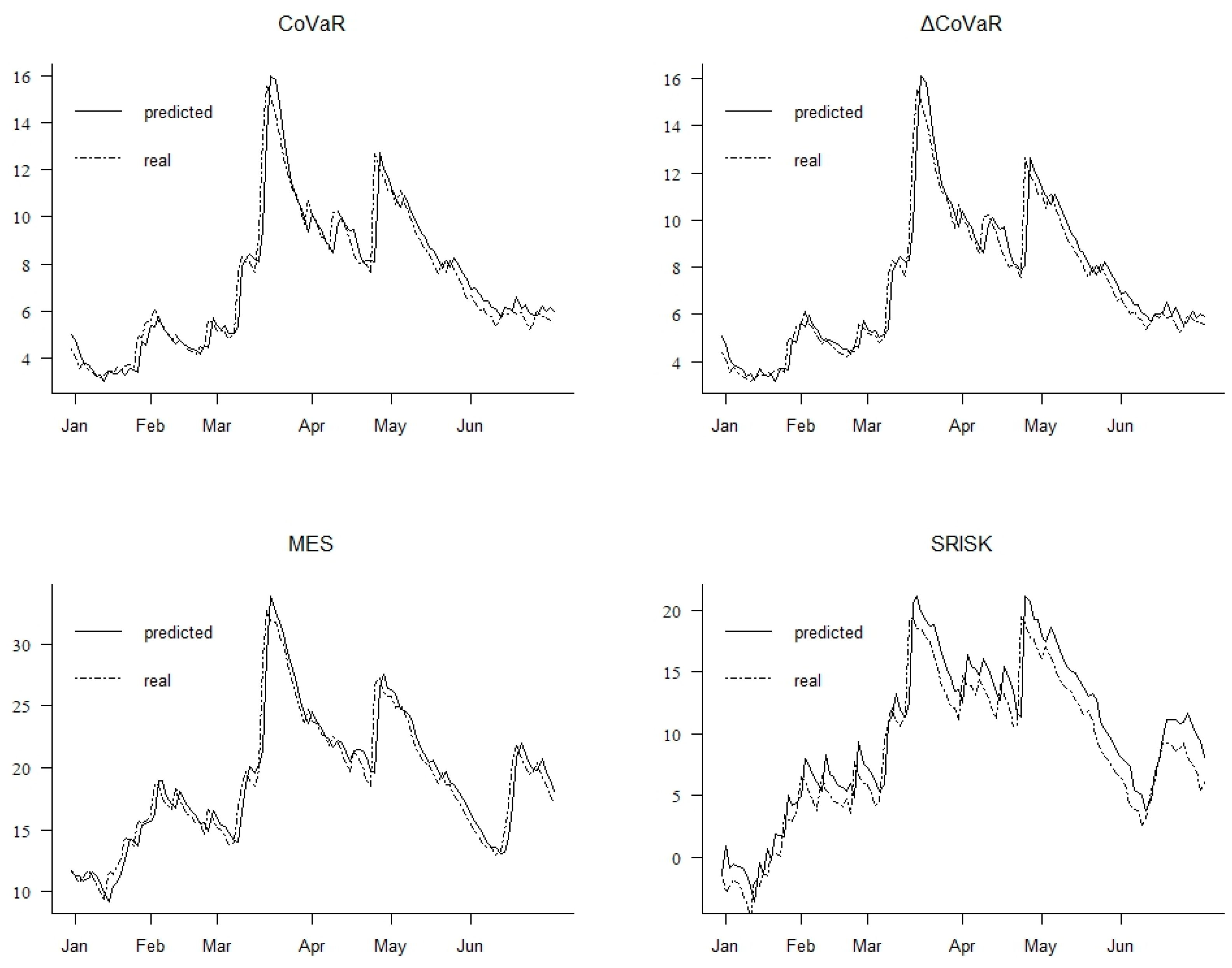
We proposed a novel ensemble model for predicting systemic financial risk. Firstly, we selected financial institutions as the research sample, measured multidimensional systemic financial risk indicators in China, and employed text mining techniques to construct a Chinese financial network public opinion index as a driving factor for predicting systemic financial risk. Subsequently, we used the ESMD method to decompose the systemic financial risk into different sub-series, and after decomposition, we reconstructed the sub-series through hierarchical clustering and FastICA methods. Finally, using the network public opinion index as input, we employed a BiLSTM-Attention ensemble model to predict different sub-series and integrate them. By evaluating the learning results, we verified the superiority of our proposed model in financial time series prediction. Our research conclusions are as follows:

Firstly, there is an interrelationship between the network public opinion index and systemic financial risk, and this interrelationship exhibits asymmetry. Specifically, the influence of the network public opinion index on systemic financial risk is much greater than the influence of systemic financial risk on the network public opinion index, indicating that the network public opinion index can serve as a driving factor for predicting systemic financial risk.

Secondly, combining data decomposition–reconstruction with deep learning methods can improve the prediction accuracy of systemic financial risk. Compared to empirical mode decomposition and variational mode decomposition, ESMD can overcome disadvantages such as mode mixing and parameter selection, making it more effective in exploring nonlinear data. Additionally, reconstructing the decomposed sub-series not only enhances prediction accuracy but also shortens the prediction time, providing a new research approach for financial time series prediction.

Thirdly, the ensemble model is more effective in predicting systemic financial risk compared to single machine learning models and traditional statistical models. Traditional statistical models fail to capture the nonlinear relationships of systemic financial risk, while single machine learning models such as support vector regression and decision tree regression, as well as single neural network models, have limitations in handling complex financial sequences. By combining bidirectional long short-term memory neural networks with attention mechanism, our predictive model gains discriminative capabilities, thus improving prediction accuracy.

Although our study has achieved certain results, there are still two main limitations. Firstly, there are limitations in the scope of the research. We selected Chinese financial institutions as the research sample, without considering different economies, various financial markets, different types of financial risks, or multidimensional influencing factors other than the network public opinion index, which may affect the research results. Secondly, there are limitations in the research methods. We constructed deep learning models for predicting systemic financial risk from a point prediction perspective based on historical time series, but the evaluation perspective can be further expanded. Therefore, as a research extension, we plan to select different economies and markets as research samples to predict various financial risks such as systemic financial risks, imported financial risks, and credit risks. We also intend to include interval prediction, model sensitivity analysis, model effectiveness evaluation, and statistical demonstration of the significance of predictive models to improve the research on financial risk prediction.