Abstract
This study investigates a symmetric fractional-order epidemic model with time delays and non-monotonic incidence rates, considering two viral strains. By confirming the existence, uniqueness, and boundedness of the system’s solutions, the research ensures the model’s well-posedness, guaranteeing its mathematical soundness and practical relevance. The study calculates and evaluates the equilibrium points and the basic reproduction numbers and to understand the dynamic behavior of the model under different parameter settings. Through the application of the Lyapunov method, the research examines the asymptotic global stability of the system, determining whether it will converge to a particular equilibrium state over time. Furthermore, Hopf bifurcation theory is employed to investigate potential periodic solutions and bifurcation scenarios, highlighting how the system might shift from stability to periodic oscillations under certain conditions. By utilizing the Adams-Bashforth-Moulton numerical simulation method, the theoretical results are validated, reinforcing the conclusions and demonstrating the model’s applicability in real-world contexts. It emphasizes the importance of fractional-order models in addressing epidemiological issues related to time delays (), individual heterogeneity (m, k), and memory effects (), offering greater accuracy compared with traditional integer-order models. In summary, this research provides a theoretical foundation and practical insights, enhancing the understanding and management of epidemic dynamics through fractional-order epidemic models.
1. Introduction
In recent years, despite improvements in medical facilities and preventive policies, many infectious diseases continue to cause significant mortality among affected populations. In order to effectively tackle this issue, it is essential to control infection transmission, shorten the duration of infections, reduce contact rates within the population, and manage host populations, among other important factors. Mathematical modeling plays a critical role in epidemiology, helping us gain a deeper understanding of epidemiological phenomena and identify crucial factors leading to severe outbreaks of infectious diseases worldwide. Despite significant advancements in medicine, leveraging research in mathematical epidemiology remains necessary to determine optimal control measures, thereby reducing the risk of disease transmission and ultimately eliminating the threat of infectious diseases. In mathematical epidemiology, researchers employ various models to probe the complexity of behaviors and nonlinear phenomena associated with diseases. These models often include three primary groups: the susceptible (S), the infectious (I), and the recovered/removed (R), collectively known as SIR models. The earliest classical mathematical model dates back to 1760, proposed by Bernoulli. The original SIR model, developed by McKendrick and Kermack [1], elevated the study of infectious diseases to a new level. Due to the long latency periods of many diseases, an additional compartment [2,3,4], known as the exposed compartment, was introduced in mathematical modeling. During the exposed period, individuals are in the latent phase but are not infectious.
In order to describe the transmission rates of diseases, we have formulated several nonlinear incidence rate functions, including bilinear incidence rates [5,6], saturated incidence rates [7], fractional incidence rates [8], and non-monotonic incidence rates [9]. For instance, Capasso and Serio (1978) [10,11,12] introduced a saturated incidence rate expressed as , where indicates infectivity, and the denominator term accounts for the suppression effect on the behavior of the susceptible population when the number of infected individuals becomes substantial. Bentaleb and Saha (2023) [13,14] introduced a non-monotonic incidence pattern given by , where k represents the psychological impact on the susceptible population. These models are suitable for depicting the infection dynamics of large populations. In many mathematical models, the bilinear transmission rate , as well as the conventional incidence rate [15,16,17,18], effectively capture the frequency of new infections per time period. Nonlinear incidence rate functions play a vital role, particularly when the number of infected individuals is substantial, by decreasing the rate of interactions between infected and susceptible individuals through quarantine measures for the infected or protection for the susceptible, thus controlling disease spread.
Recent research has made progress in dual-strain SIR and SEIR models [19,20], involving bilinear and non-monotonic incidence rate functions. For example, Baba and Hincal (2017) [21] proposed a dual-strain SIR model with a bilinear transmission rate for a single strain and a non-monotonic transmission rate for the additional strain, demonstrating the global stability of all equilibria using the basic reproduction number. Bentaleb and Amine (2019) [22] expanded on this work by introducing exposure compartments for both strains, confirming the global stability of all equilibrium types and illustrating the principle of competitive exclusion in ecology, where the strain with the higher basic reproduction value can outcompete and eliminate the other strains. Subsequently, Meskaf et al. (2020) [23] further extended these studies by adopting a non-monotonic incidence rate. In order to establish the global stability of the equilibrium states, various Lyapunov function theorems were applied. Many researchers have conducted multi-strain studies on different epidemic models [20,24,25,26].
In order to effectively simulate the spread of diseases, especially when accounting for various types of time delays, such as latent and immune periods, an increasing number of studies have introduced time-delay differential equations [27,28,29,30,31,32,33,34]. These delays include delays related to the immune response and not only the latent period. Furthermore, the theory of optimal disease control under different delayed conditions is also considered. For example, Amine Murugadoss Zhu et al. [32,35,36,37] have incorporated two delays into a dual-strain model, conducting dynamic analysis, bifurcation studies, and control theory research under various incidence rates. Additionally, fractional-order differential equations [38,39,40], due to their intrinsic inclusion of memory effects and nonlocal impacts, have been widely used in epidemiological models. They offer several advantages in biological modeling by capturing long-term dependencies, such as latency and recovery periods in infectious diseases, and by flexibly and robustly handling complex systems characterized by multiple scales and nonlinear feedback. Furthermore, fractional-order equations can naturally simulate the sub-dynamic behaviors of nonlinear phenomena such as reaction rates, diffusion, and growth, thus providing a powerful tool for modeling complex biological systems. For instance, Zhou and Barman [41,42] considered incubation period delay as a bifurcation parameter and analyzed the existence of Hopf bifurcations in both time-delay SIR models and time-delay nonlinear SEIR models, further investigating the characteristics of these bifurcations. This approach deepens our understanding of the complexities of disease transmission and the response to strategic interventions.
The arrangement of this paper is as follows: Section 2 reviews the basics of fractional-order differential equations and introduces key lemmas. Section 3 analyzes a dual-strain fractional-order SEIR model featuring two non-monotonic interaction functions. In Section 4, we provide a comprehensive mathematical evaluation of the model, including its non-negativity and boundedness properties, calculate the basic reproduction number, and prove the global stability of the equilibrium points. Section 5 conducts a brief bifurcation analysis. Finally, Section 6 presents numerical simulation results and summarizes the research findings.
2. Basic Knowledge
In this subsection, we will review the key definitions, relevant lemmas, and important theorems associated with fractional calculus.
Definition 1
([43]). For a function , the fractional derivative of order in the Caputo sense is defined by the following expression:
Here, refers to the set of functions that are n times continuously differentiable over the interval . The term denotes the Gamma function, and m is a positive integer such that . Additionally, ξ is greater than . For the specific case where , the Caputo fractional derivative is defined as follows:
Definition 2
([44]). For any complex number, y, the Mittag-Leffler function is defined in two forms. The single-parameter Mittag-Leffler function is given by the following formula, while the two-parameter Mittag-Leffler function is defined as follows:
where and .
Lemma 1
([45]). Suppose is a continuous and differentiable function; then,
where , .
Lemma 2
([46]). Let and with . Then, there exists such that
Lemma 3
([47]). Consider a continuous function with . Suppose this function meets the following criterion:
Under these conditions, the inequality is given by
for every , where represents the single-parameter Mittag-Leffler function, which is defined as follows:
Lemma 4
([48]). Consider as an equilibrium point within the subset Ω of .
and assume is a function that is continuously differentiable and satisfies the following condition:
for and , with () being functions defined on Ω that are both continuous and positive definite. Then, is uniformly asymptotically stable.
Theorem 1
([49]). Assume , where is a domain and is a function that satisfies the Lipschitz criterion with respect to ξ. Review the fractional-order system presented here:
given the initial state , a unique maximal solution exists for the system.
Theorem 2
([50]). Examine the following fractional-order system with m dimensions and delay:
For and , the system might undergo a Hopf bifurcation near the equilibrium state when the delay τ equals a critical value , given that the following criteria are fulfilled:
- (A)
- The arguments of all eigenvalues of the coefficient matrix in the linearized system are such that .
- (B)
- When , the characteristic equation of the system has a pair of purely imaginary roots, specifically .
- (C)
- Re , here represents the real component of a complex eigenvalue.
3. Model Formulation
By building on existing research and being inspired by previous work [23,35,51], our study focuses on a delayed dual-strain epidemiological model with non-monotonic incidence rates. The goal is to examine the dynamic effects of suppression between different strains in the model. To this end, we employ the following set of nonlinear differential equations to describe the system:
subject to the initial conditions:
where are all non-negative.
Using fractional-order models provides a more precise depiction of the true dynamics within complex systems [52,53], especially in fields such as epidemic spread, material diffusion, and economic dynamics. These models not only enhance the descriptive power of theoretical frameworks but also offer new perspectives and tools for analyzing and solving real-world problems. However, when transitioning from ordinary differential models to fractional-order models, an issue of order mismatch arises between the two sides of the equation. In order to address this, we modify the parameters on the right-hand side of the equation, expressing them in fractional form. The fractional-order model is formulated as follows:
subject to the initial conditions:
In order to rigorously capture the dynamic behavior of infectious diseases involving multiple strains using the dual-strain fractional-order SEIR model, it is crucial to ensure that models (1) and (3) satisfy the conditions or . Establishing these conditions forms a solid foundation for conducting more precise theoretical and numerical analyses in the subsequent study of the model’s dynamic evolution.
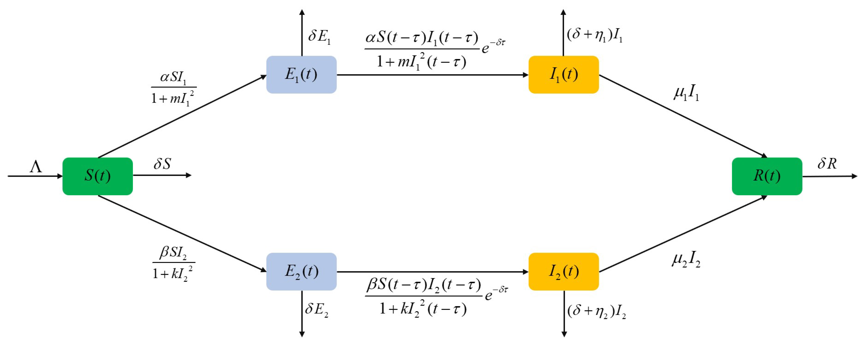
The above model equation contains six variables. S represents the susceptible population, while and represent the latent populations for strains 1 and 2, respectively. and denote the infected populations for strains 1 and 2, in that order, and R represents the removed individuals. Table 1 provides the biological interpretations of the various parameters used in the model. A diagrammatic explanation of the dual-strain fractional-order SEIR model is presented in Figure 1.

Table 1.
Details of the parameters of model (3).
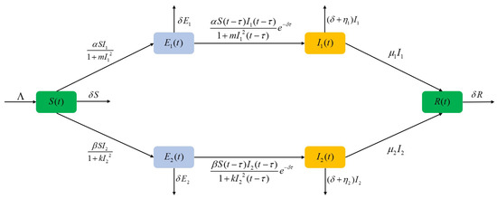
Figure 1.
Representation of the two-strain fractional-order SEIR model.
4. Model Analysis
This section focuses on proving the well-posedness of the system by verifying the existence, positivity, and boundedness of the solutions. Additionally, we confirm the presence of a single disease-free equilibrium state and three local disease equilibrium points: the first and second local disease equilibrium points and the coexistence disease equilibrium point. We derive the formula for the basic reproduction number and determine the possible steady states. Subsequently, we prove the stability of these equilibrium states using appropriate Lyapunov functionals.
4.1. The Presence and Singularity of Solutions
The subsequent lemma will be used to demonstrate the existence and uniqueness of the system’s solution.
Lemma 5.
We will examine the fractional-order system outlined below:
where , . Provided that adheres to the Lipschitz criterion in terms of z, a solution to the system exists on .
Theorem 3.
For any point in the system, there exists a unique solution
for all .
Proof.
First, consider the interval where
Here, and K are two finite positive values. Next, take two points and in and suppose a mapping such that .
With
When considering all , we have the following:
where , with . Consequently, fulfills the Lipschitz condition for , ensuring that the system admits a unique solution
given the initial condition . Thus, the theorem is proved. □
4.2. Positivity and Boundedness
Non-negativity and boundedness constraints are essential for accurate ecological and biological models, providing a reliable foundation for ecology, epidemiology, demography, and related fields. Therefore, the solutions of system (3) must conform to these requirements.
Theorem 4.
The fractional-order system (3) with the given initial condition (4) ensures a unique solution. Moreover, all solutions to the system (1)–(3) exhibit positivity, boundedness, and convergence to a compact attractor.
Proof.
Theorem 3 has established that, given the initial condition , a unique solution exists for any t.
In order to demonstrate that , we proceed by contradiction. Suppose there exists or such that for any , , and for , , with . Here, it is assumed that is sufficiently small. Based on the first equation in system (3), we observe that
Therefore, as per Lemma 2, there exists such that
If we choose to be sufficiently small, we find that , which contradicts the assumption that for . Therefore, it follows that for .
In order to prove that , we again use proof by contradiction. Suppose there exists such that for any , and with for . Here, is assumed to be sufficiently small. Based on the second equation in system (3), it follows that
Similarly, according to Lemma 2, there exists such that
Thus, contradicts the assumption that for . Therefore, for all , .
In order to prove that , we again use proof by contradiction. Suppose there exists such that for any , and with for . Here, is assumed to be sufficiently small. Based on the fourth equation of system (3), it follows that
According to Lemma 2, there exists such that
This leads to , which contradicts the assumption that for . Thus, for any , .
Based on the above analysis for the compartments S, , and in the system, it can similarly be shown that , , and .
Next, let us continue to prove boundedness.
In order to prove boundedness, we adopt the following definition:
The fractional derivative of is given by
Thus, we obtain . From Lemma 3, this implies that
where . The limit exists, and we have
Hence, the solutions of the system are always bounded, leading to the positive attractor set of system (3) being
With this, the theorem is proven. □
4.3. Basic Reproduction Number ()
The basic reproduction number refers to the average number of new infections generated by a single infected person in a completely susceptible population, commonly denoted by . The classic method to derive the expression for is through the next-generation matrix method, . is determined by the formula [54], where represents the largest eigenvalue (spectral radius). Here, H is the non-negative matrix representing new infections, and F is the transfer matrix associated with model (3). The next-generation matrix is precisely .
In relation to system (3), since the first, fourth, and fifth equations do not depend on the variables , , and R, the model can be reduced to the following subsystem:
Clearly, holds consistently for system (6). Thus,
So,
In order to determine the basic reproduction number, we use . This implies that
where
4.4. Feasible Equilibria
Four equilibrium states characterize model (3): one where the disease is absent and three where the disease persists endemically. In order to determine the effective equilibrium point, where the variables in the system remain constant over time, the derivatives of all state variables at the equilibrium point must equal zero; we examine the situation where system (3) has a zero value on its right-hand side:
resulting in the following:
- Model (3) always has a disease-free equilibrium . When , the equilibrium point satisfies the following equation:
- The equilibrium point where strain 1 persists when and , whereand is a root satisfying the following equation:with .
- The equilibrium point where strain 2 persists when and , whereand is a root satisfying the following equation:with .
- The combined endemic equilibrium for the two strains exists when and , whereand and are solutions to the following system of equations:where
4.5. Global Stability of the Systems’ Equilibrium States
Here, our goal is to verify the global stability of the equilibrium state. In order to achieve this, we will employ suitable Lyapunov-type tools to establish the system’s global stability.
Theorem 5.
The condition and ensures that the disease-free equilibrium point is globally asymptotically stable.
Proof.
Define the Lyapunov function in the following manner:
It is now apparent that is strictly positive throughout all , , , , , and . Then,
Substitute system (6) into the above expression, then simplify it to obtain
The conditions detailed in the discussion are
and hence
We consider the following scenario:
- For any , we have .
- For any , we have .
Then, if and hold, then is true.
From the above discussion, we can infer that if and hold, then , with .
It is concluded that the disease-free equilibrium achieves global asymptotic stability when and . □
Theorem 6.
The global asymptotic stability of the strain 1 endemic equilibrium is guaranteed when and .
Proof.
Define the Lyapunov function in the following manner:
Here, (). Observe that reaches its lowest strict global value at . For further validation, let and . Thus, we obtain and .
Then, the fractional derivative of is given by
By substituting system (6) into the above expression, we obtain , where .
Then,
Next, let us discuss the properties of each formula:
For the equation , due to the properties of , we have
For the equation , due to , , , and , we have
In addition, we have the following equation:
Finally, for the expression , we assume that the function satisfies the following condition:
In summary, let us discuss two scenarios:
- If , then , so . Additionally, for , we have , which implies that .
- If , then , so . Furthermore, for , we have , which implies that .
Based on the previous discussion, it follows that if , then .
Therefore, it can be established that the endemic equilibrium corresponding to strain 1 is globally asymptotically stable, provided that and . □
Theorem 7.
The global asymptotic stability of the strain 2 endemic equilibrium is ensured when .
Proof.
Define the Lyapunov function in the following manner:
Here ().
Then, the fractional derivative of can be expressed as
By substituting system (6) into the above expression, we obtain and .
Then,
Next, let us discuss the properties of each formula:
For the equation , due to the properties of , we have
For the equation , due to the , , and , we have
In addition, we have the following equation:
Finally, for the expression , it is accepted that the function adheres to the following requirement:
In summary, let us discuss two scenarios:
- If , then , so . Additionally, for , we have , which implies that .
- If , then , so . Furthermore, for , we have , which implies that .
Based on the previous discussion, it follows that if , then .
Therefore, it can be established that the endemic equilibrium , corresponding to strain 2, is globally asymptotically stable, provided that . □
Theorem 8.
The global asymptotic stability of the combined endemic equilibrium is guaranteed if and , thus indicating .
Proof.
Define the Lyapunov function in the following manner:
Here, ().
Then, the fractional derivative of can be expressed as
By substituting system (6) into the above expression, it can be readily demonstrated that
Then,
Next, let us discuss the properties of each formula:
For the expression , due to the properties of , we have
Assume that satisfies the condition ; then, . For the expression
For the expression
Assume that satisfies the condition ; then, . We have
Additionally, we have the following:
- When , we have , and then .
- When , we have , and then .
By combining the above assumptions, the following scenarios can be considered:
- If , we have .
- If , we also have .
From the above discussion, we can conclude that whether or , the condition is always satisfied. Hence, the system reaches global asymptotic stability at the steady state if . □
5. Local Hopf Bifurcation Examination
This segment is dedicated to studying local stability and investigating the occurrence of local bifurcations at the endemic equilibrium in the two-strain model. At the endemic equilibrium point , the characteristic equation for model (3) is expressed as
where
with ; ; ; ; and .
Case 1: We assume that . Then, Equation (9) becomes
where
In addition, assuming the conditions and are satisfied, there exist and , where and . Clearly, , so we let . Therefore, based on the Routh-Hurwitz criterion theory, the following assessments hold:
Based on the above steps and theoretical analysis, if the conditions in Equations (11)–(15) hold, then the endemic equilibrium state of the system without delay (system (3)) exhibits local asymptotic stability.
Case 2: In the case where , we multiply both sides of Equation (9) by to obtain
Assume () is an imaginary root of Equation (16). By substituting () into Equation (16) and isolating the real and imaginary components, we obtain
where
Further, Equation (17) results in
with
Since , we have
where
Define . Then, Equation (20) can be rewritten as
For ease of analysis, we can further assume that Equation (21) has a positive root. Thus, Equation (16) will necessarily have a pair of purely imaginary roots if Equation (21) exhibits a positive root. Therefore, the threshold value of the delay with respect to can be obtained.
Furthermore, taking the -derivative of both sides of Equation (16) leads to
where
In the end, we get
Undoubtedly, if holds, then . With reference to the earlier discussion and Hopf bifurcation theory, as discussed in [36,41], we derive the following conclusions:
Theorem 9.
If the condition is fulfilled, then the following results are valid:
- (i)
- For τ values in the range , the equilibrium state of system (3) exhibits asymptotic stability.
- (ii)
- A Hopf bifurcation is observed in System (3) at its real equilibrium point at .
Equation (22) defines .
6. Numerical Simulations
A series of numerical simulations will be carried out in this section. Given the complexity of the analytical solutions, numerical analysis is particularly necessary. This study uses MATLAB R2018b to perform simulations that visually demonstrate some of the theoretical results presented in earlier sections of this paper. The initial conditions for the simulations are , , , , , and . The parameters are adjusted according to various dynamic changes. The Adams-Bashforth-Moulton method [29,55] has been proven to be an efficient and powerful technique for solving fractional-order ODEs. It is used in MATLAB to perform simulations with variations in the system’s fractional order , time delay , and inhibitory parameters m and k. These simulations help analyze the dynamic behavior of susceptible and infected populations under different strains. In order to better observe the system’s dynamics, some parameters are modified during the simulation process. Table 2 lists the parameter values used for each numerical result.
Table 2.
The parameter values of the fractional order SEIR two-strain model.
6.1. Dynamic Analysis of Different Equilibrium Points in the System due to Changes in Order
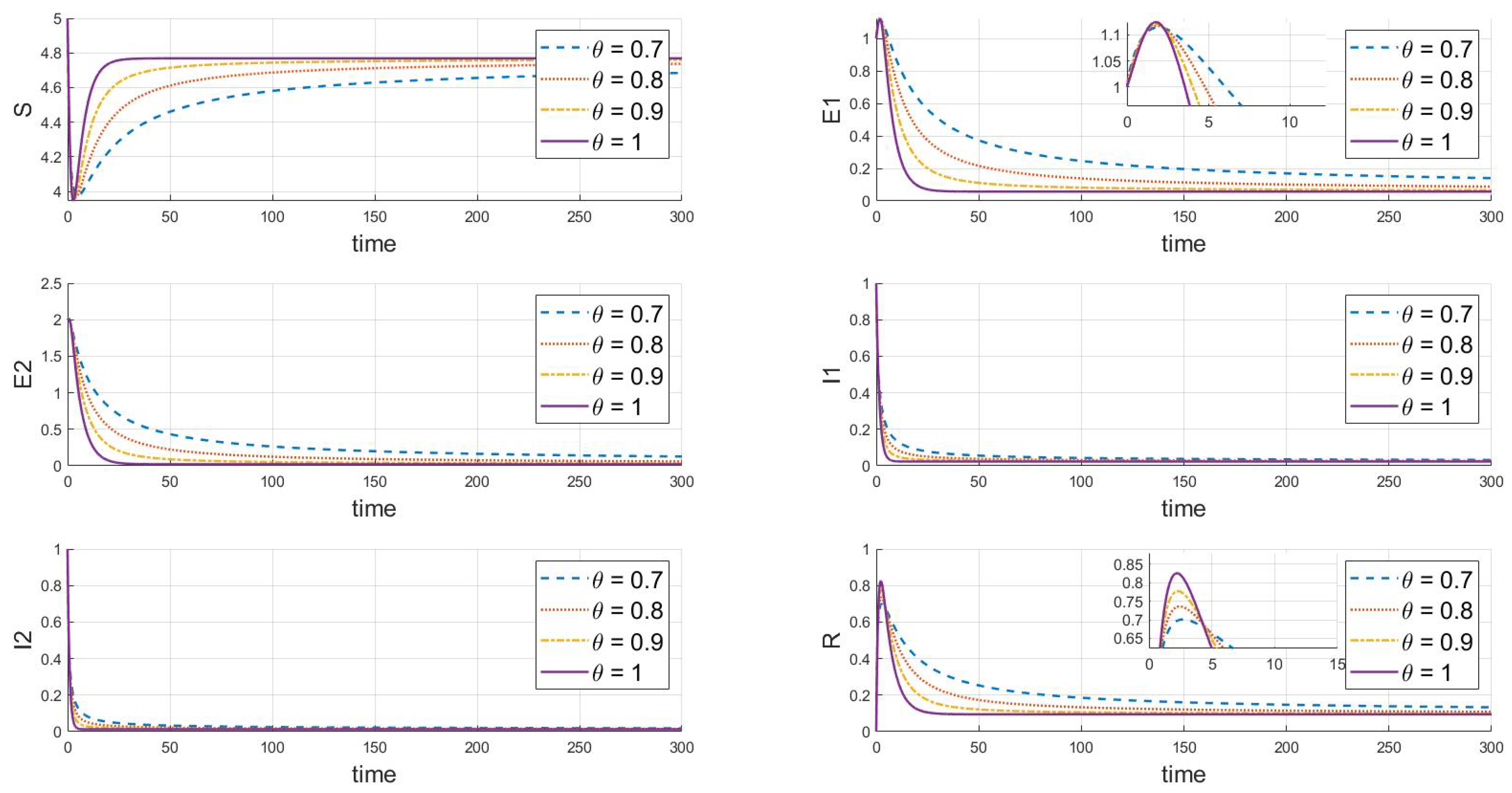
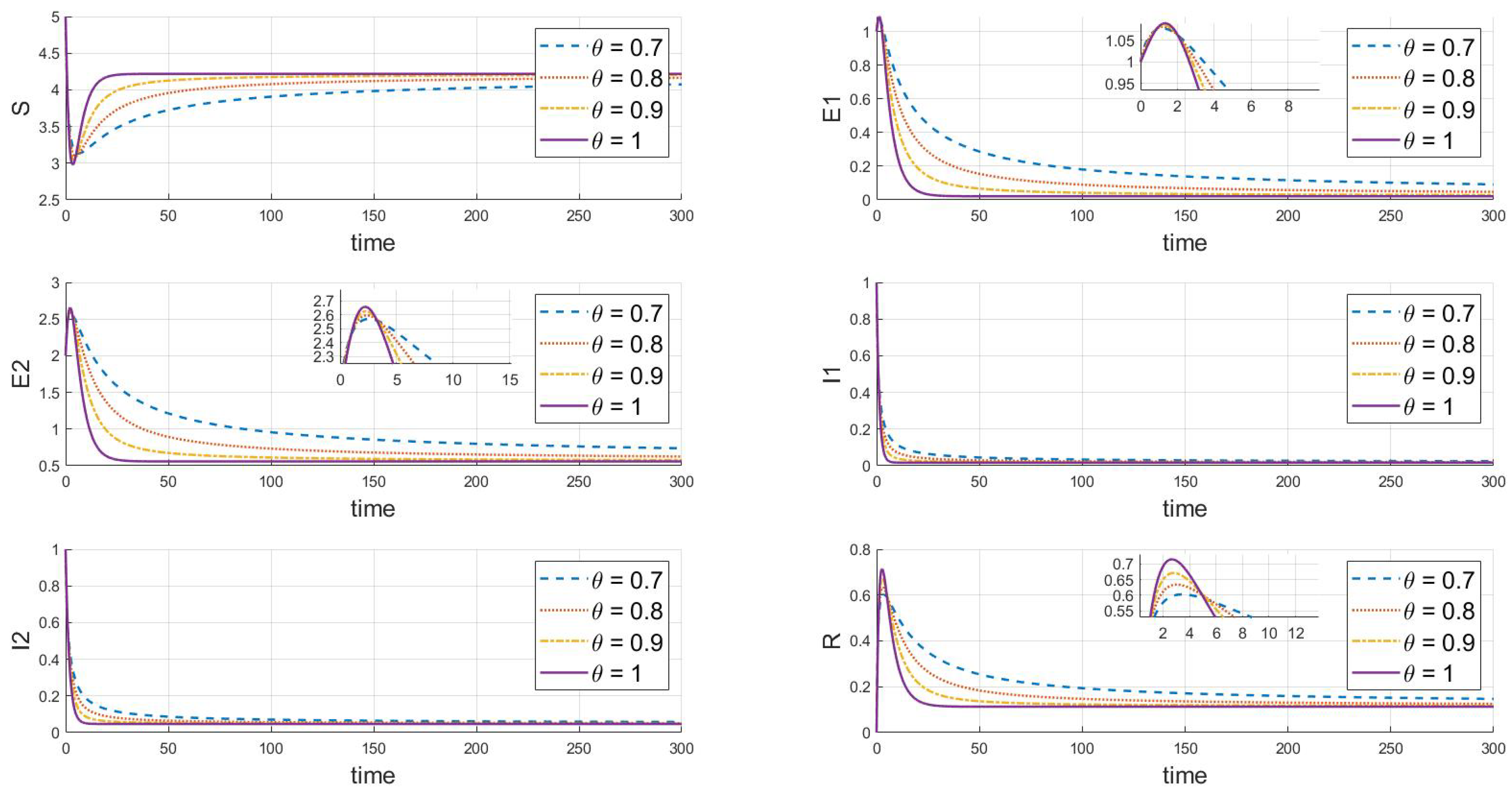
According to the parameter values from Table 2, stability analysis theory clearly shows (in Figure 2) that the disease-free equilibrium is stable under different values of , where and . This indicates that both strains will eventually disappear. The figure also demonstrates that different values of significantly affect the dynamics, peak sizes, and rates of change in each compartment. As the parameter increases, the rate of change over time of the system’s state variables (including susceptible, exposed, infected, and recovered individuals) accelerates, particularly with a significant increase in the speed at which the system reaches a steady state. A higher value corresponds to a faster decay in the disease transmission process, indicating weaker memory effects and quicker system stabilization.
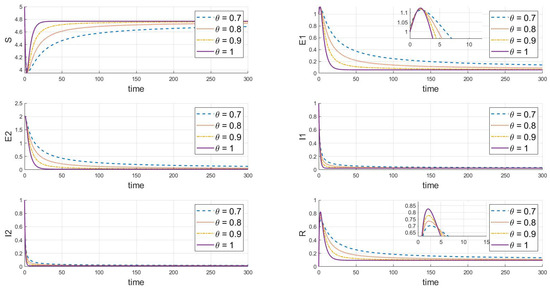
Figure 2.
When and , this is the effect of varying on the steady state of the system.
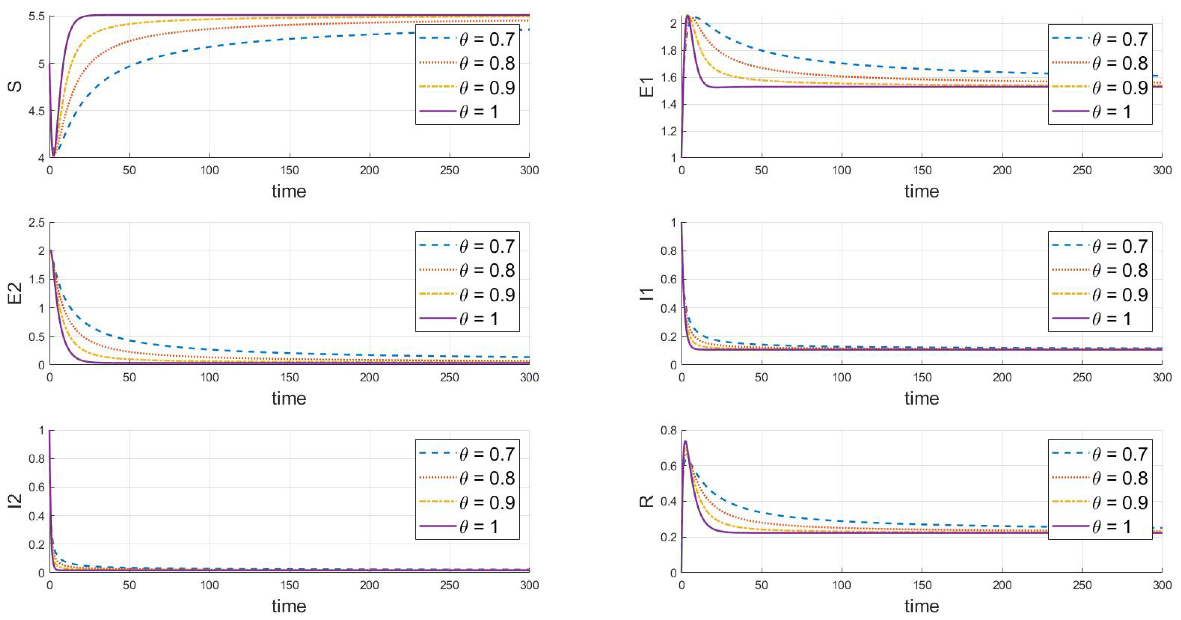
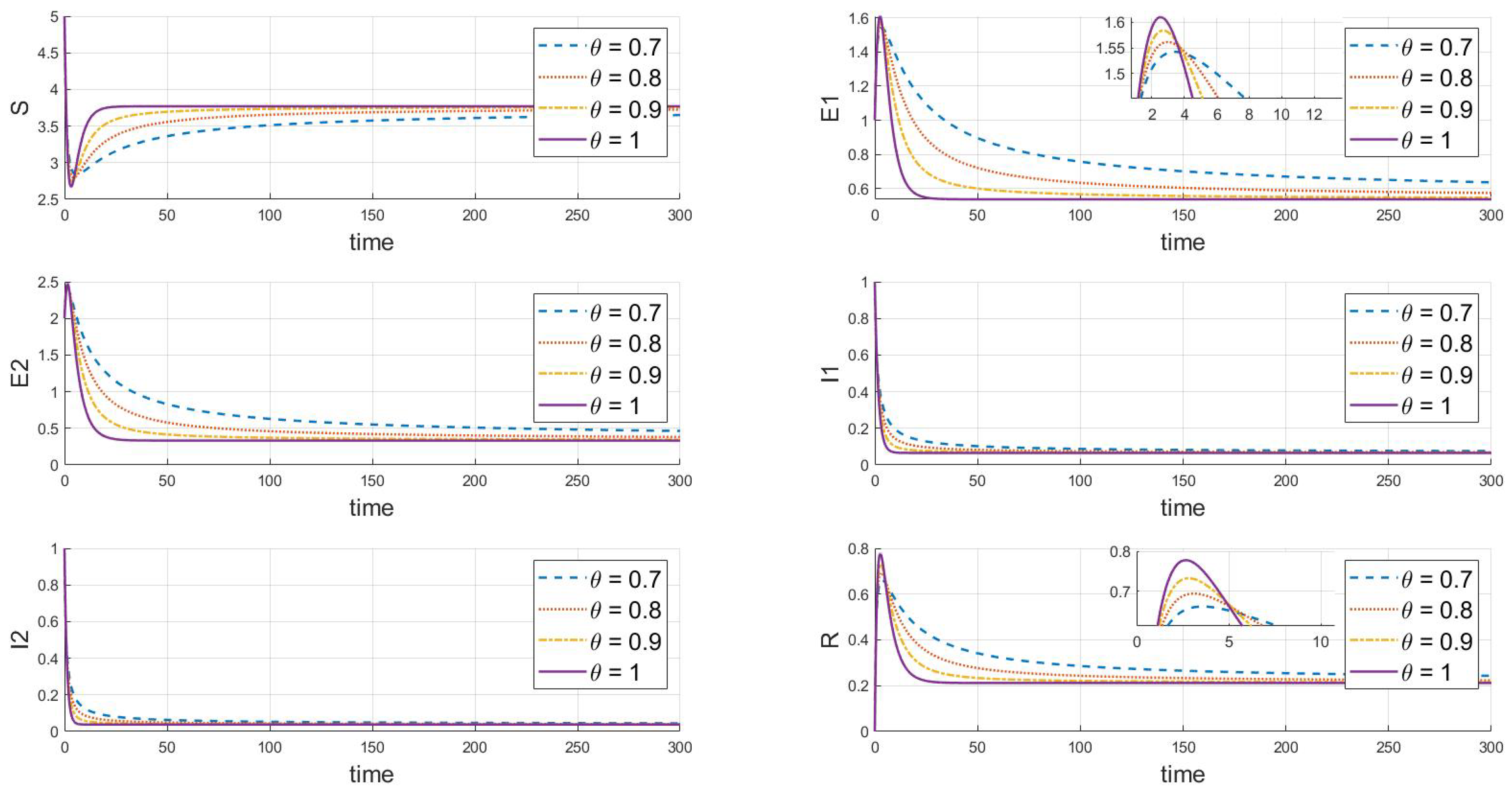
Adjustments to the parameters reveal the endemic equilibrium state of strain 1, where and , as shown in Figure 3, which gradually stabilizes under various values. It is evident that strain 1 will persist and stabilize, while strain 2 will ultimately vanish or even become extinct. As increases, the speed at which the system reaches a steady state significantly increases, with a more pronounced effect on the reduction of infected individuals and the increase in recovered individuals.
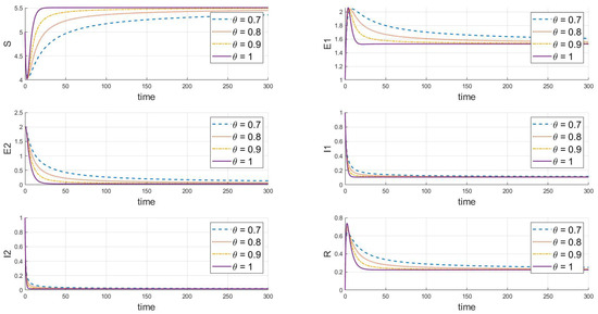
Figure 3.
When , this is the response of the system’s steady state to changes in .
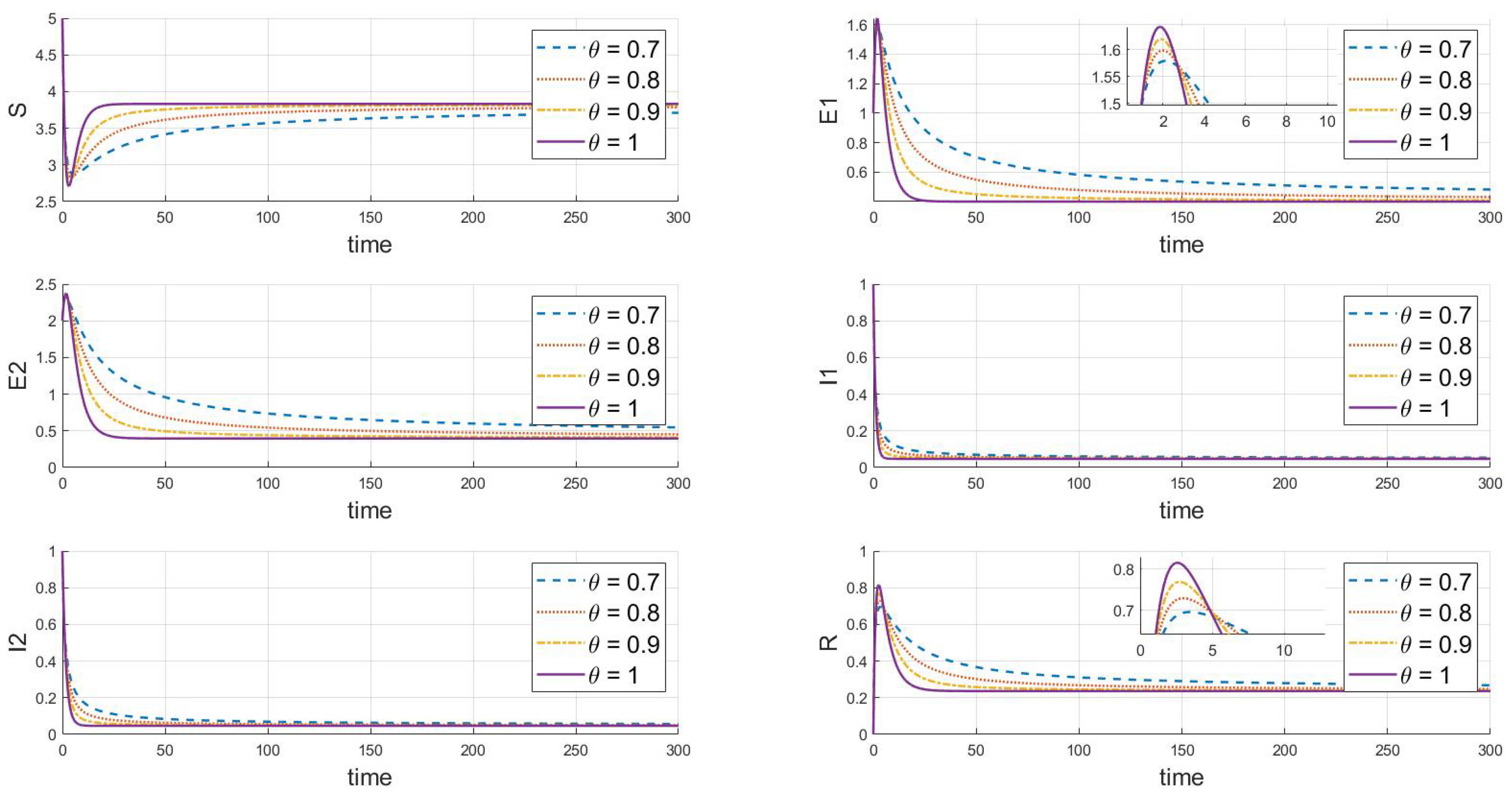
Further adjustments indicate the endemic equilibrium state of strain 2, where and , as depicted in Figure 4. The system always tends toward a stable state under different values; given that the basic reproduction number of strain 2 is greater than 1, it will continue to exist and remain stable, while strain 1 will gradually disappear. As shown in the dynamic behavior from the figures, changes in the fractional-order parameter significantly affect the convergence speed of each state variable in the system. As increases from 0.7 to 1, the time to reach the steady state shortens. This is especially evident in the evolution of the exposed individuals , , and the infected individuals , . The higher the fractional order, the faster the infection fluctuations dissipate. An increase in the fractional order reflects a reduction in the model’s memory effect, implying that at higher fractional orders, the system’s memory of previous states weakens, thus accelerating both the spread and control of the epidemic.
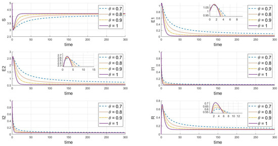
Figure 4.
When , the response of the system’s steady state to changes in .
Finally, the adjustments shown in Figure 5 () and Figure 6 () demonstrate that under different values, both strains will eventually persist and stabilize despite differences in the peak values and rates of change between the strains, likely due to differences in their transmission and infection characteristics. Additionally, when comparing Figure 5 and Figure 6 with basic reproduction numbers , we observe significant differences in the behavior of the two strains at the endemic equilibrium point. These differences are evident in the peak values of each compartment, the stable state values, and the time and rate at which stability is reached. Some strains quickly reach their peak in a short period, while others rise more slowly. In the long term, the stable state values of different strains in each compartment also vary. Furthermore, there are differences in the time and rate at which each strain stabilizes. As increases (from 0.7 to 1), the decay rate of each variable accelerates, indicating that the disease spreads more slowly within the population, and the peak infection time occurs earlier. Specifically, larger values correspond to faster disease clearance and lower infection rates. This highlights the crucial role that the memory effect of fractional derivatives plays in regulating the long-term dynamics of disease transmission.
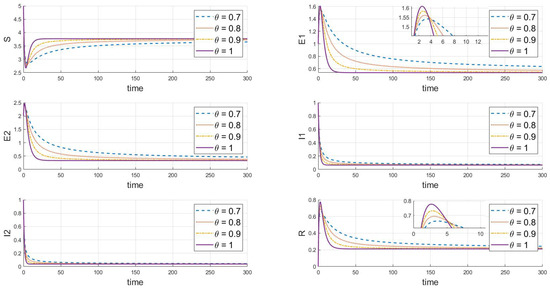
Figure 5.
When , we see the response of the system’s steady state to changes in .
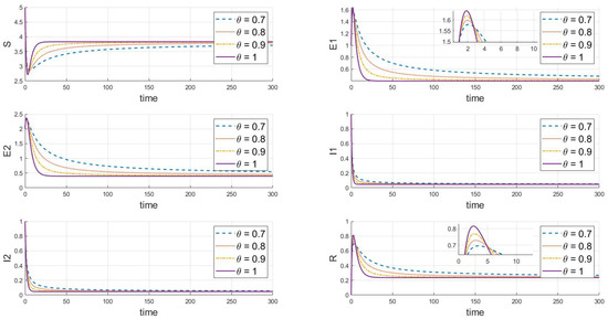
Figure 6.
When , we see the response of the system’s steady state to changes in .
Our comprehensive analysis suggests that these differences may be related to the strains’ transmission cycles, immune evasion capabilities, and treatment effects. It is also hypothesized that the strains may influence each other’s transmissibility and dynamic changes. These differences become more pronounced at different fractional orders, reflecting the complex dynamics of disease transmission. Overall, the system maintains a continuously stable state at different equilibrium points, and the variation in values significantly impacts the dynamics of the infectious disease model, particularly affecting the peak values, the timing of these peaks, and their trends. These simulation results help us understand the effectiveness of disease control strategies, especially when considering different rates of transmission and treatment effects.
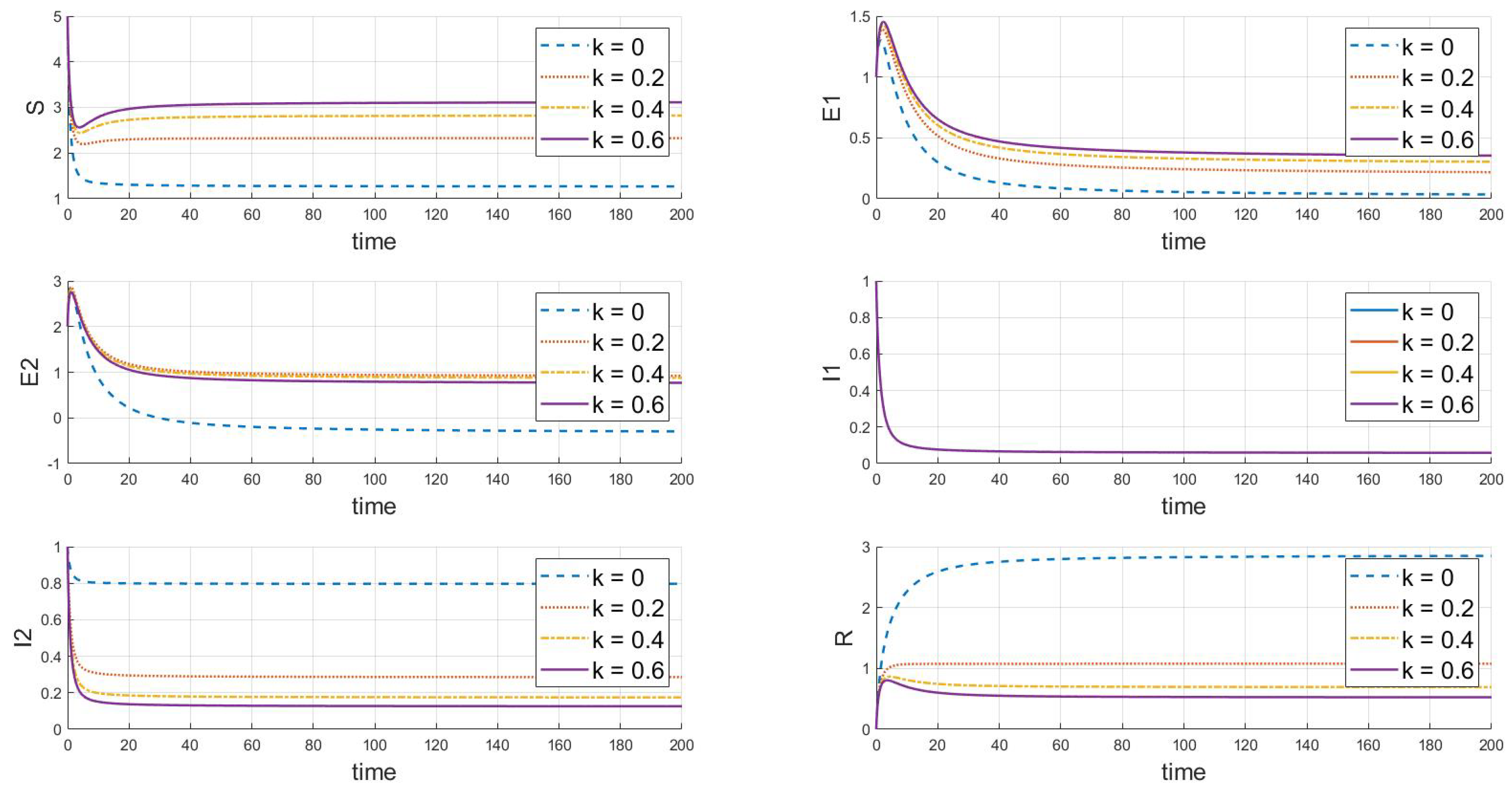
6.2. The Impact on the System Due to Changes in the Parameters That Measure the Psychological or Inhibitory Effects of Different Strains
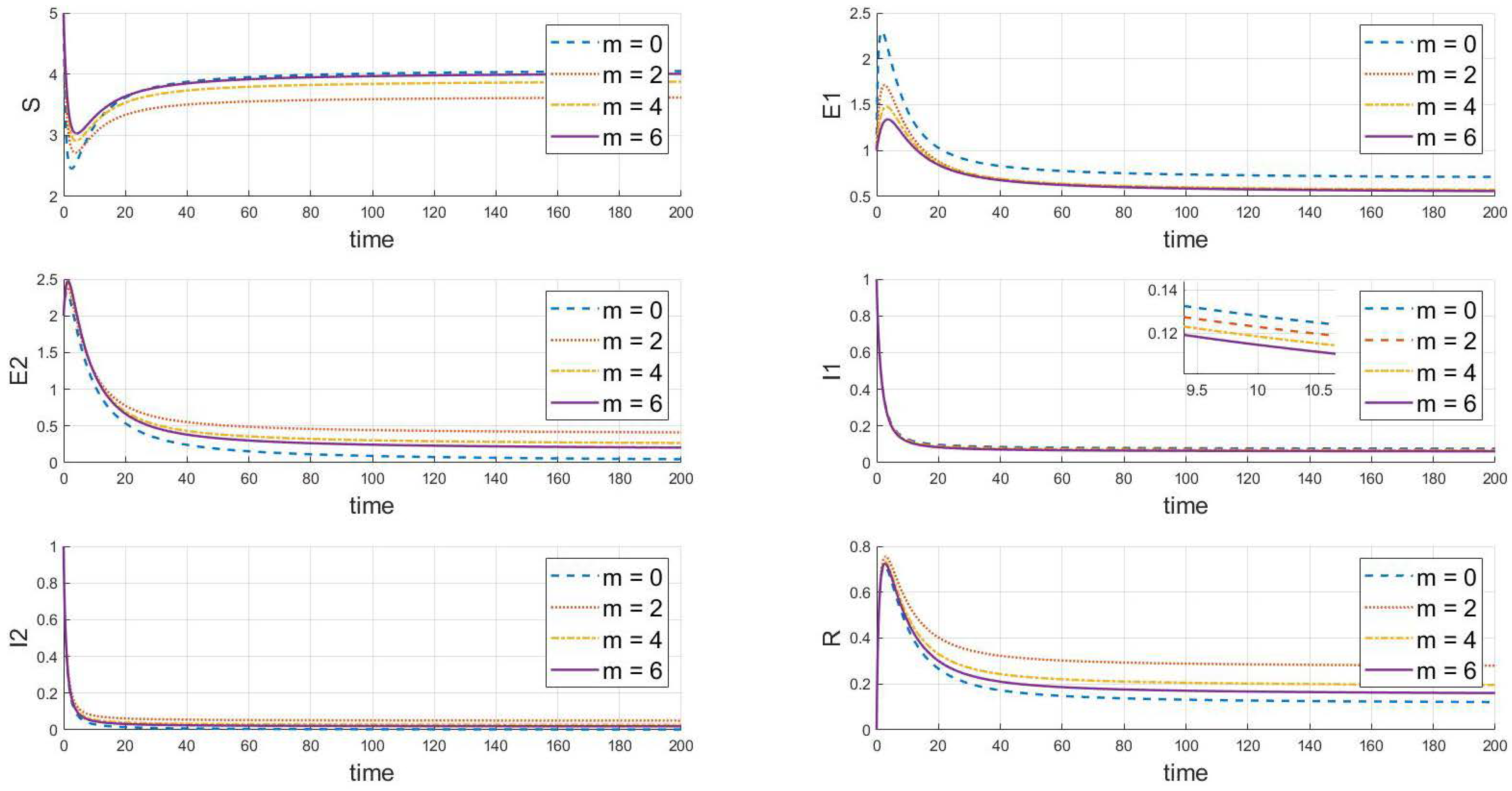
Based on the analysis of parameters, the influence of parameters m and k on the system’s group dynamics is elaborated as follows: firstly, Figure 7 reveals that as parameter m grows, the initial decline in the number of susceptibles decreases, indicating that enhanced containment measures effectively slow the spread of the virus. A higher value of m also allows the number of susceptibles to nearly return to its initial level after an initial drop, reducing the loss of susceptibles and prolonging the presence of exposed individuals. This slows the decline in the number of exposed individuals and, thus, lowers the peak of the outbreak. Simultaneously, the peak of infected individuals occurs later, is lower, and the recovery rate is faster, demonstrating that strong containment strategies significantly control the scale of the outbreak. In Figure 8, as the value of k increases, the decrease in the number of susceptibles is less pronounced, indicating that containment measures slow the transmission of the disease among susceptibles, prolong the transition of exposed individuals to infected status, reduce the peak in infections, and result in a lower peak in recoveries, indicating that fewer people are infected. In summary, increasing the values of m and k simulates more effective containment measures, which slow the spread of the disease, reduce the scale of outbreaks, and effectively control the impact of the epidemic.
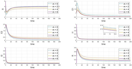
Figure 7.
The dynamic impact of changes in parameter m, which represents the psychological or inhibitory effect of strain 1 on the system.
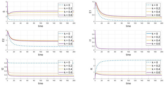
Figure 8.
The dynamic impact of changes in parameter k, which represents the psychological or inhibitory effect of strain 2 on the system.
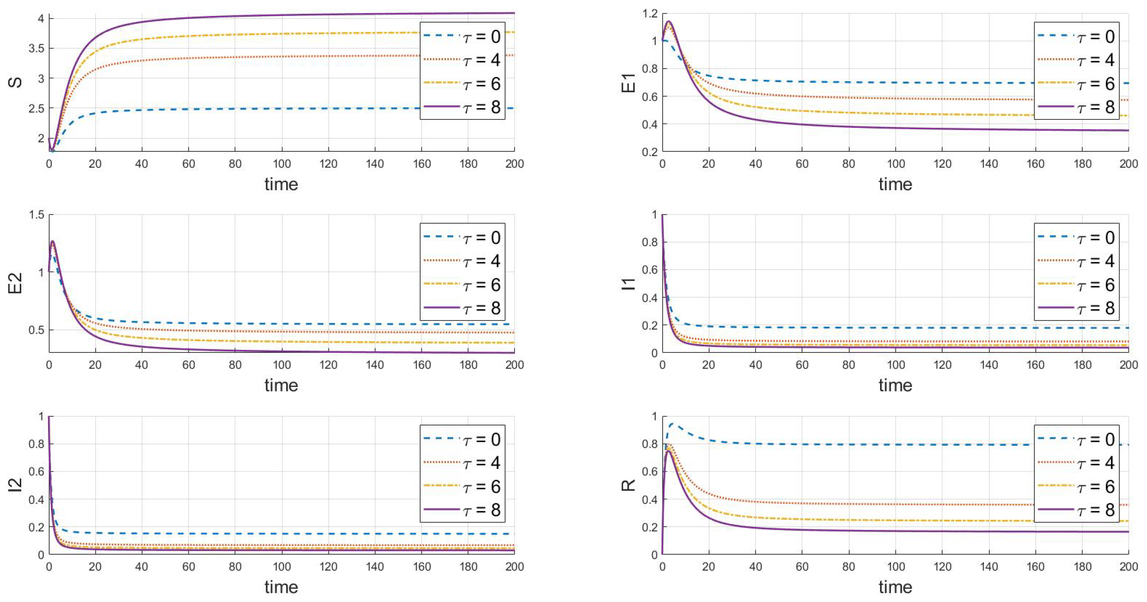
6.3. The Impact of Variations in Time Delays on the Dynamics of the System
Based on the analysis of the parameters from Table 2, the impact of the delay parameter on the dynamics of the system’s populations is summarized as follows in Figure 9:
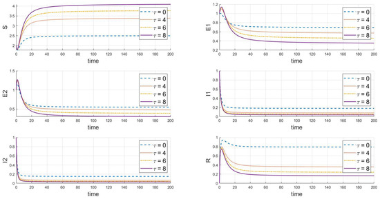
Figure 9.
The dynamic impact of variations in the delay parameter on the system.
Firstly, as the delay increases, the rate of decrease in the susceptible population slows down, ultimately stabilizing at a higher level, indicating that delay measures can partially protect susceptible individuals. Secondly, the number of exposed individuals initially declines rapidly, but as increases, this decline slows down. Additionally, the increase in also causes the peak of infected individuals to appear later and at a lower height, indicating that the speed of infection clearance is slower, and it takes longer to control the epidemic. Finally, a larger causes the recovered population’s peak time to shift later and the peak height to drop, reflecting that despite the delayed implementation of control measures, the overall number of infections decreases, easing the pressure on recovery and indicating a long-term trend in the epidemic.
In summary, the increase in the delay leads to a delayed response in disease dynamics. This analysis is crucial for understanding the impact of extended latency periods or the delayed implementation of intervention measures on disease control strategies, and it aids in developing more effective disease management strategies.
6.4. Hopf Bifurcation Exists and Analysis
By building on the theoretical bifurcation analysis discussed above, these numerical simulations highlight the effects of combining fractional-order dynamics with time delay regarding the system’s steady-state and periodic responses. For the parameters used in the numerical simulations, we select , , , , , , , , , and . Given the relationship between the basic reproduction number and the delay parameter , changes in delay will always affect the basic reproduction number. Numerical calculations have confirmed that this holds true for both and . Therefore, the evolution of the system’s dynamics at the endemic equilibrium point will be analyzed in more detail. In order to illustrate the specific impact of bifurcation theory on disease dynamics, this section primarily explores the changes in the number of individuals in the susceptible and infected compartments through numerical analysis.
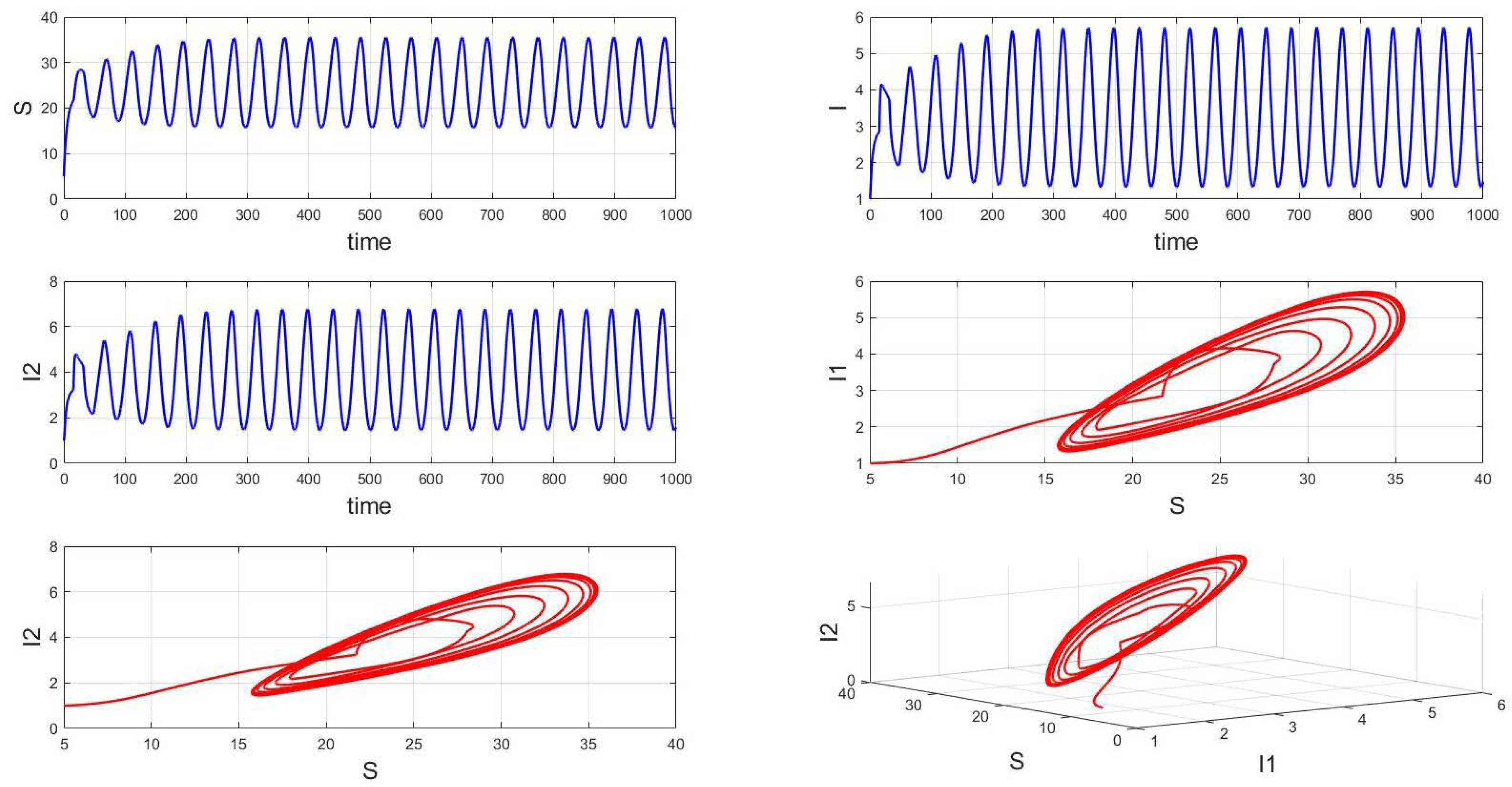
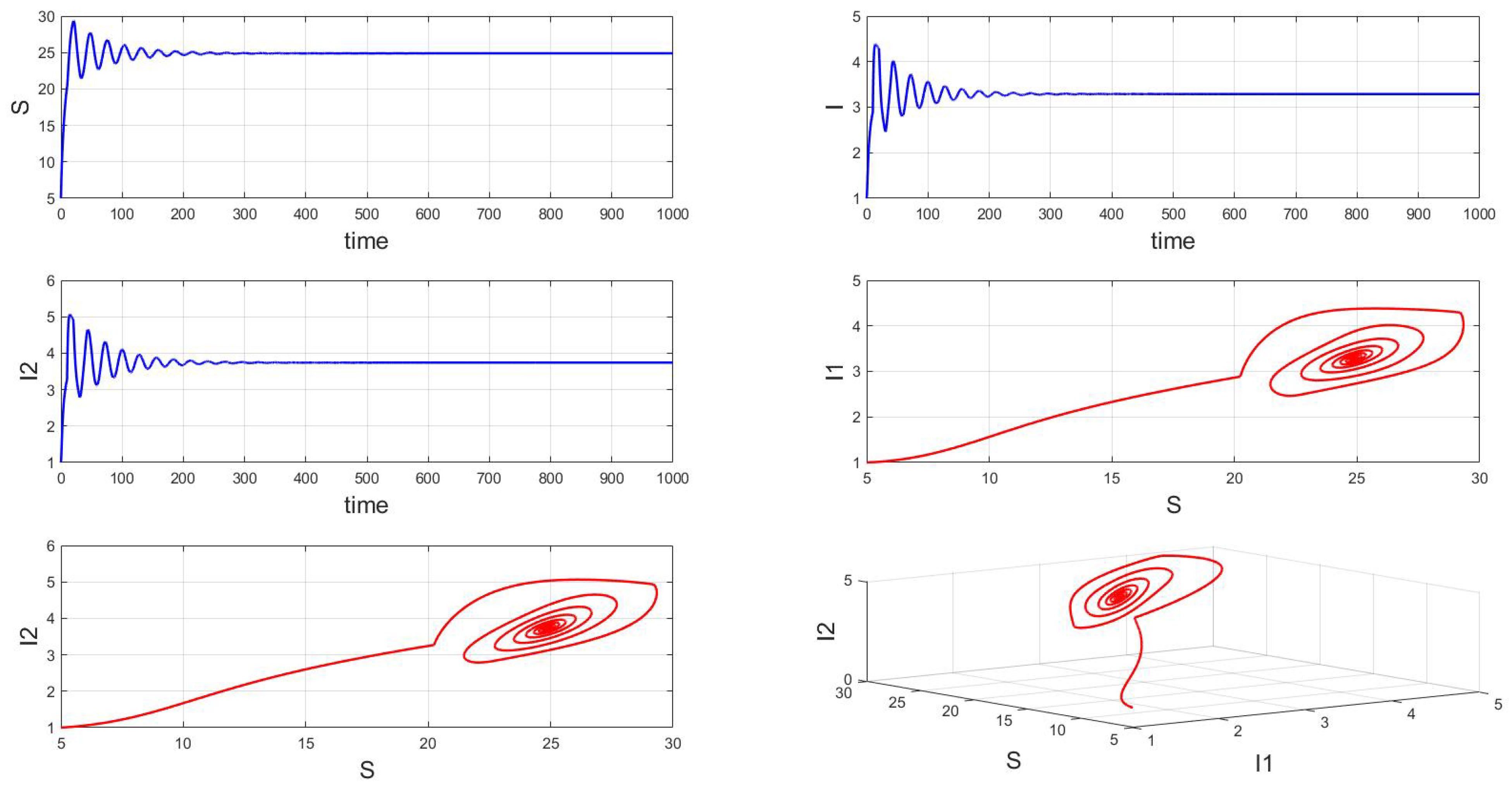
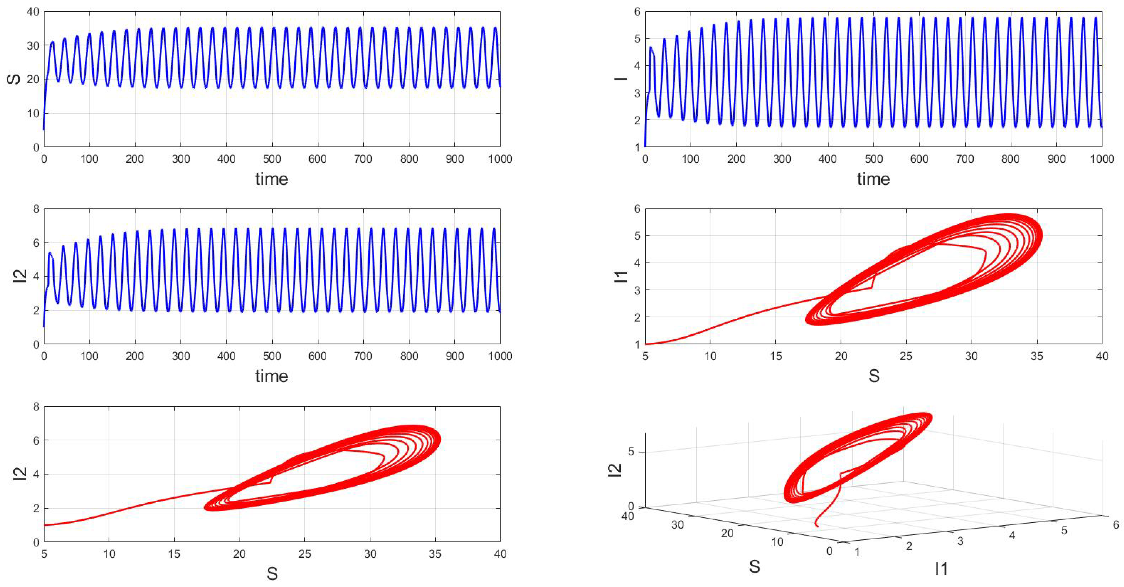
For a system with a fixed order of 0.95, different delays are chosen. As shown in Figure 10, when is selected, the system exhibits asymptotically stable dynamics at the endemic equilibrium point. Moreover, based on the analysis, we can infer that as the parameter increases from 11 to 12.5, the system undergoes a bifurcation from a stable fixed point to a periodic orbit, exhibiting a typical Hopf bifurcation phenomenon. This implies that when the parameter or crosses a critical value , the system loses stability, undergoes a Hopf bifurcation, and stable periodic solutions emerge, as illustrated in Figure 11, Figure 12 and Figure 13. Therefore, when the infectious disease system enters a periodic state, it may necessitate adjusting the timing and intensity of control measures to effectively manage peak transmission periods. Monitoring changes in delay parameters and analyzing shifts in system dynamics can forecast future transmission trends and potential cyclic outbreaks. This is crucial for designing effective strategies in antimicrobial resistance management and vaccine deployment to ensure sustained and effective disease control and prevention.
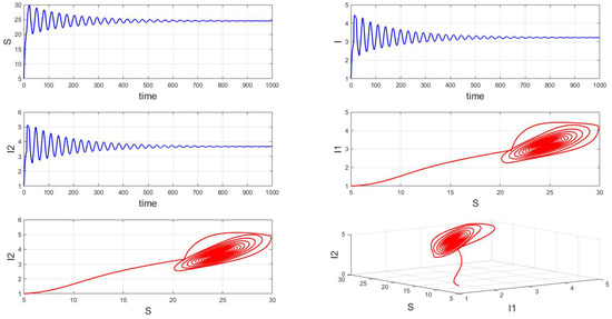
Figure 10.
Waveform diagrams and phase plots of the system with .

Figure 11.
Waveform diagrams and phase plots of the system with .
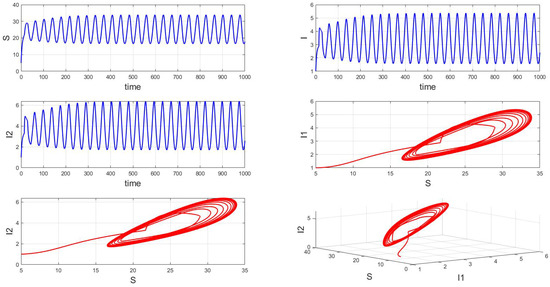
Figure 12.
Waveform diagrams and phase plots of the system with .
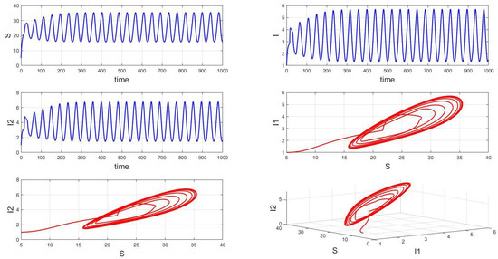
Figure 13.
Waveform diagrams and phase plots of the system with .
When the fixed parameter is , the analysis reveals the following dynamics: when in integer-order systems, the endemic equilibrium point will be locally asymptotically stable, as depicted in Figure 14. However, upon crossing a critical value of the order , an intriguing phenomenon emerges: the system gradually loses stability, undergoes a Hopf bifurcation, and presents the formation of stable periodic patterns, as illustrated in the transition from Figure 15 () to Figure 16 (). Fractional-order derivatives allow for greater flexibility in capturing long-term memory effects and complex dynamic evolution within systems. This flexibility can lead to the gradual destabilization of the system, culminating in a Hopf bifurcation. Analyzing the impact of fractional-order derivatives on system stability and periodic solutions enables more precise predictions of long-term transmission trends and potential outbreaks of infectious diseases, aligning more closely with the realistic transmission characteristics observed in practice.
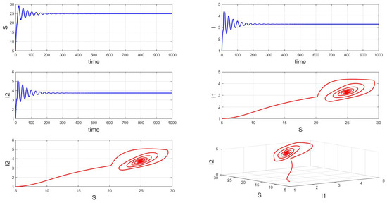
Figure 14.
Waveform diagrams and phase plots of the system with .
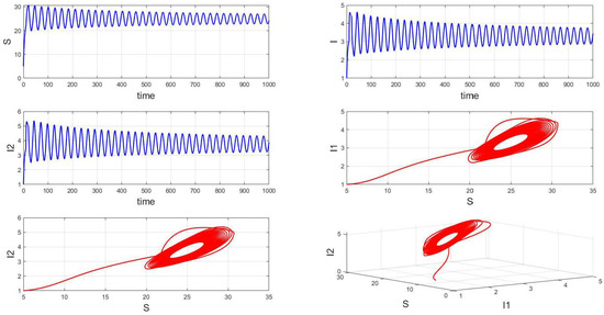
Figure 15.
Waveform diagrams and phase plots of the system with .
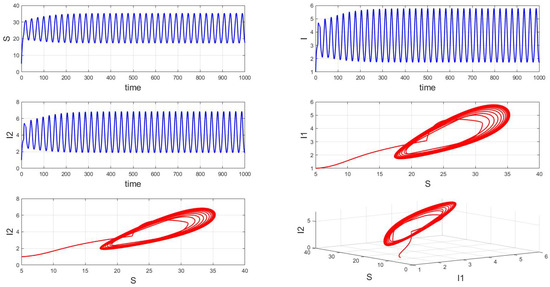
Figure 16.
Waveform diagrams and phase plots of the system with .
Through numerical simulations, we have observed various intriguing dynamic phenomena resulting from changes in system parameters. Specifically, under the combined influence of these parameters, the system exhibits stable periodic solutions, meaning that, under certain conditions, the system’s state repeats in a regular manner. However, the system may also experience bifurcation phenomena, transitioning from a stable non-zero periodic solution to a stable equilibrium point. This indicates significant changes in the system’s long-term behavior.
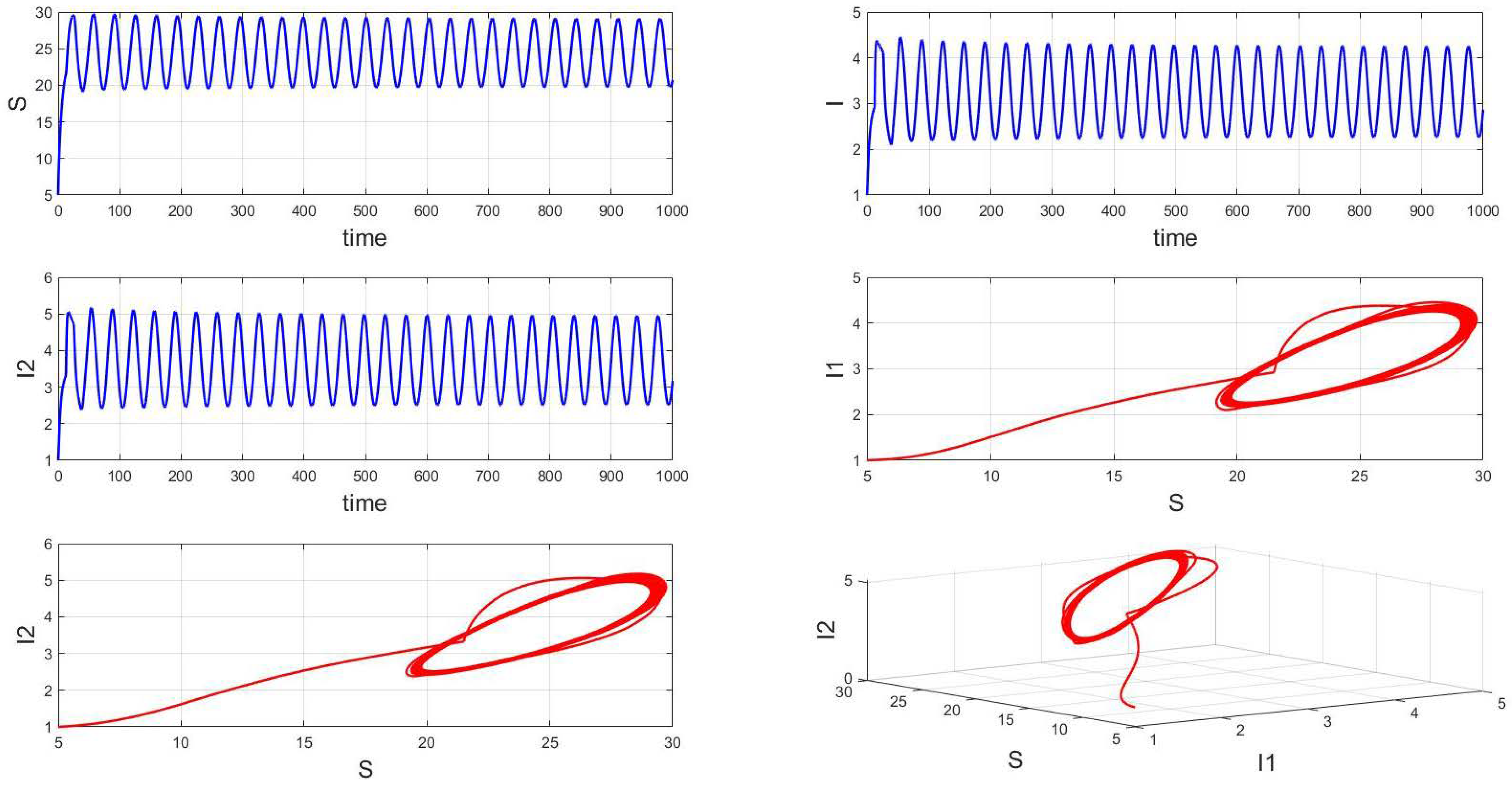
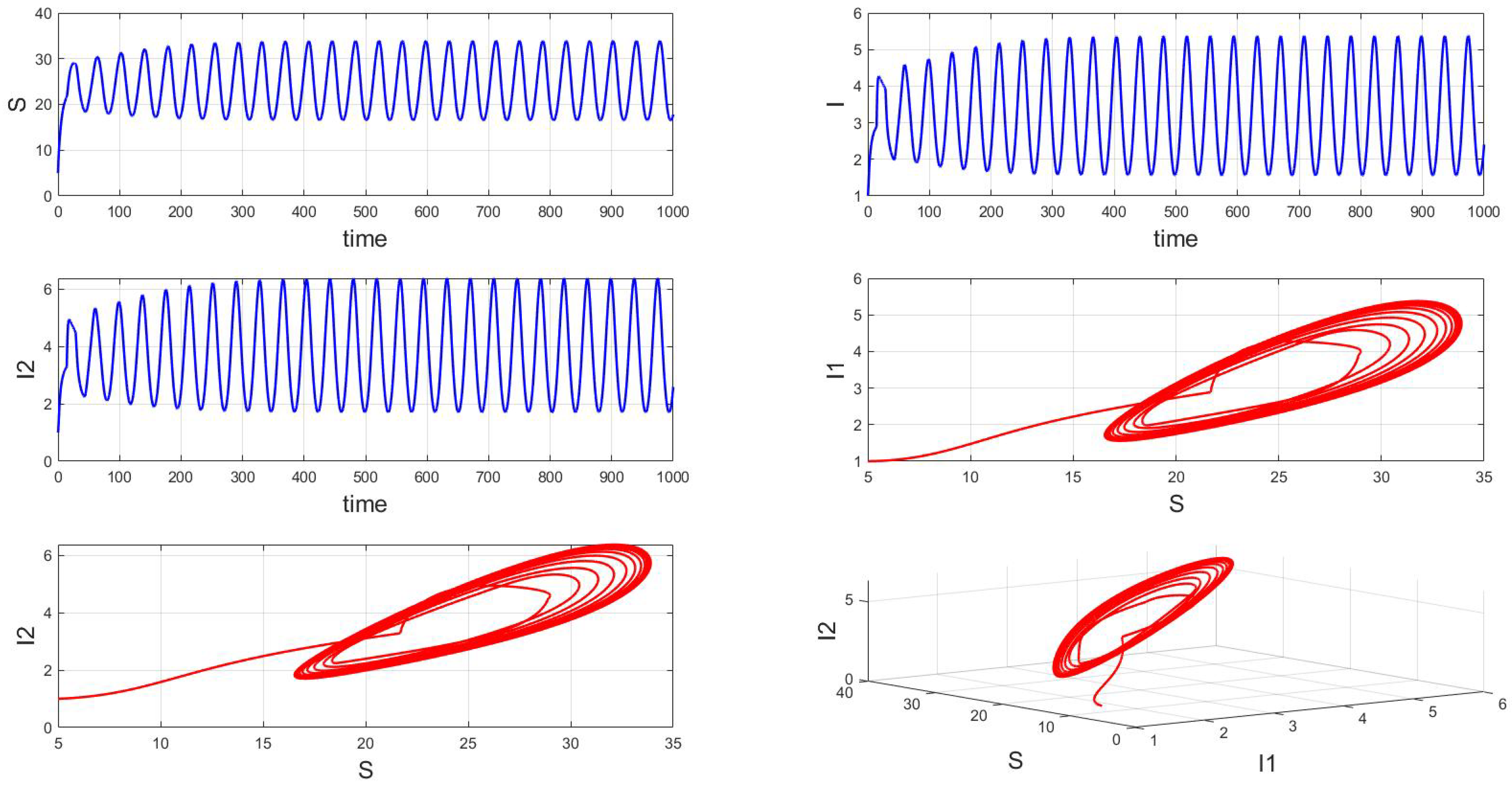
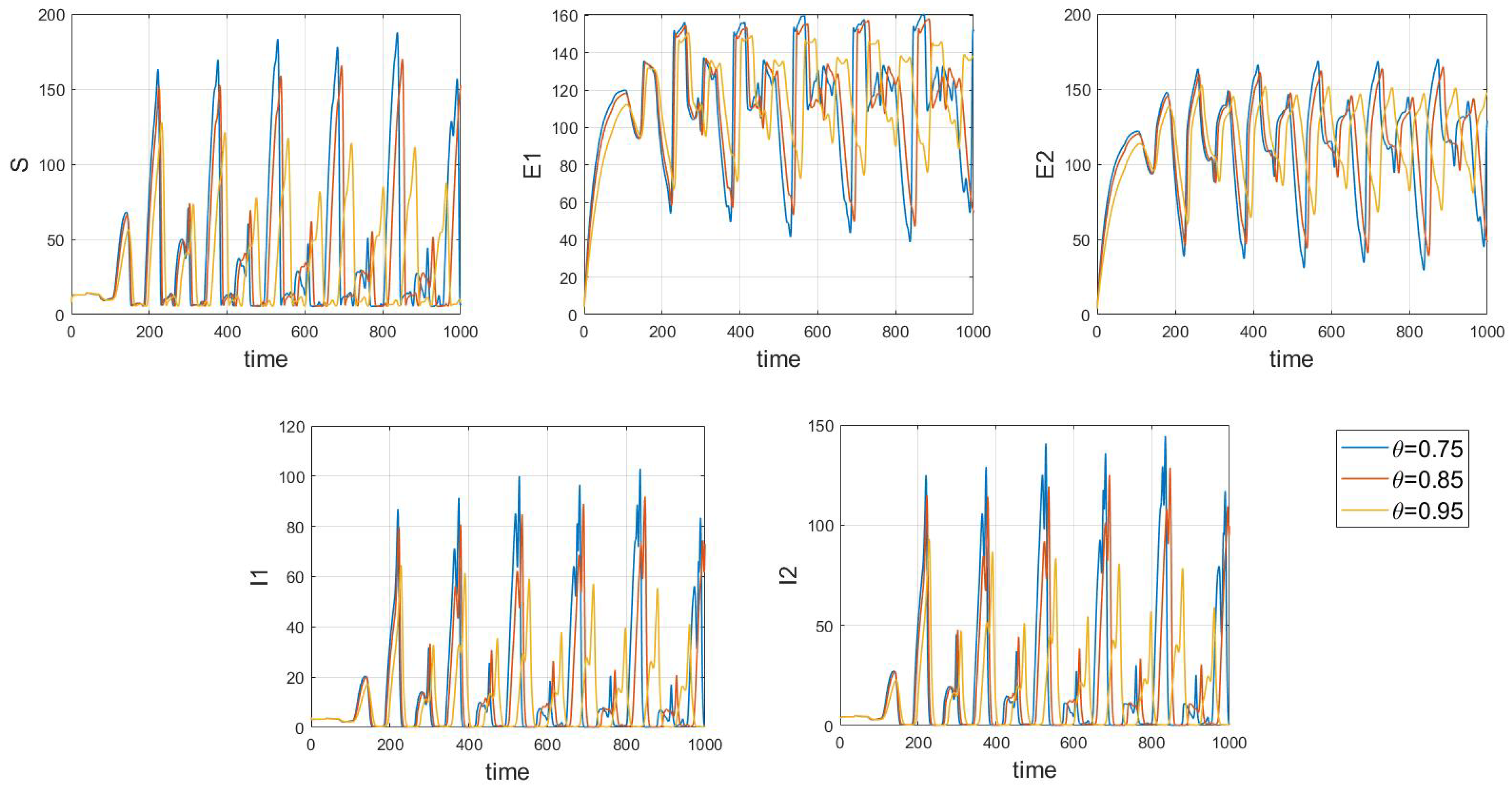
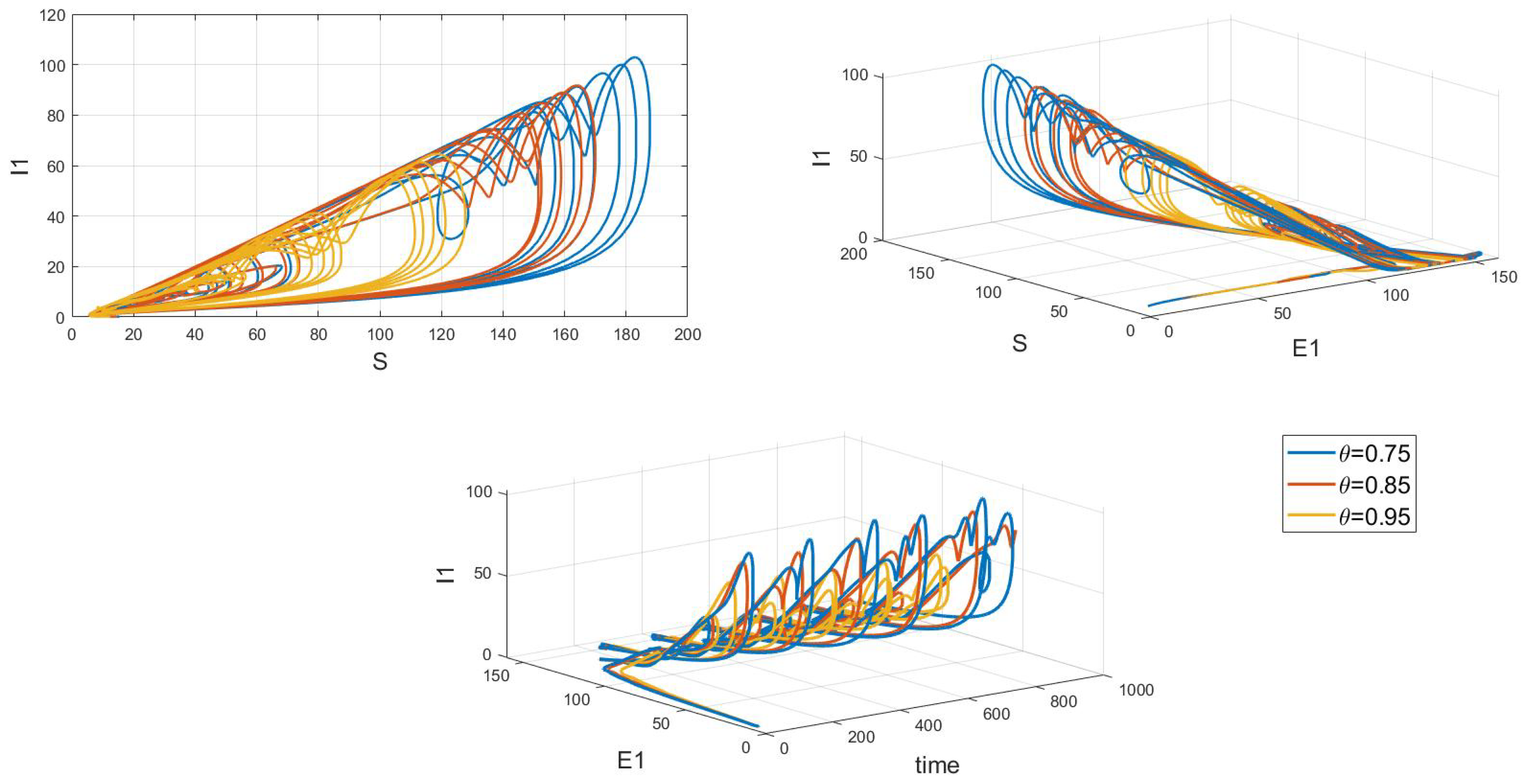
Of particular interest is how variations in the system’s initial conditions, transmission rate parameters, and psychological inhibition parameters, along with changes in delay, lead the system to gradually shift from stable periodic solutions to chaotic behavior. This clearly demonstrates bifurcation behavior, where the system’s state undergoes dramatic changes and exhibits complex dynamics. As shown in Figure 17, Figure 18 and Figure 19, these figures respectively illustrate the chaotic behavior of strain 1 and strain 2. They highlight the system’s dynamic characteristics and chaotic phenomena under different parameter settings and initial conditions.
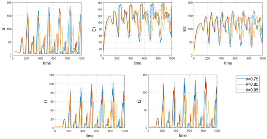
Figure 17.
Waveform diagrams and phase plots of the system with chaos.

Figure 18.
Chaos phase diagram for strain 1.
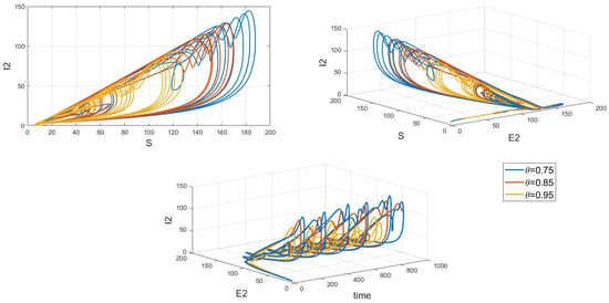
Figure 19.
Chaos phase diagram for strain 2.
Chaotic behavior in infectious disease models reveals the complexity and unpredictability of transmission dynamics. This behavior highlights the virus’s susceptibility to a range of complex factors, including intricate nonlinear interactions, variations in individual behaviors, and environmental changes. The presence of chaos implies that the system can undergo dramatic shifts and exhibit unpredictable states, making disease control more challenging. This underscores the need for designing effective disease control strategies and public health policies that account for these complex dynamics. Such strategies must not only be based on a thorough understanding of the transmission model but also be adaptable to handle the nonlinear and uncertain aspects of the system. This may involve implementing more flexible and responsive interventions, such as real-time monitoring and adjusting control measures to address system changes and emerging situations. Therefore, understanding and addressing chaotic behavior is crucial for developing scientifically sound disease control measures and enhancing the effectiveness of public health decisions.
7. Conclusions
This investigation centers on a dual-strain SEIR model utilizing fractional-order delay differential equations to control non-monotonic incidence rates. We explored the properties of non-negativity and uniqueness and conducted a global analysis using appropriate Lyapunov functions for an SEIR model encompassing two strains with non-monotonic incidence rates. By applying the next-generation matrix method, we derived the basic reproduction numbers and for the two strains, establishing the necessary and sufficient conditions for the asymptotic global stability of the four equilibrium points. Our analysis was supported by various numerical simulations. Furthermore, we discussed the Hopf bifurcation analysis concerning the delay and order , presenting key findings from the perspectives of local stability and local Hopf bifurcation. The results indicate that the model remains stable when bifurcation parameters are below critical values, facilitating disease control. However, surpassing these critical values induces Hopf bifurcations, leading to a loss of control over disease spread. Therefore, minimizing delays in the model is essential for predicting and controlling disease transmission. Similar considerations apply to the influence of the order , where adjusting the magnitude of memory effects aids in disease prediction and control. Additionally, we conducted a theoretical analysis of Hopf bifurcation properties and validated our findings through numerical simulations. The integration of delay and fractional order enhances the dynamical characteristics of epidemiological models, improving their stability.
Future research should explore how seasonal variations and climate changes impact fractional-order epidemic models, assess the effect of stochastic noise on model robustness and accuracy, investigate co-infection scenarios, and examine the influence of different vaccination and treatment interventions. Additionally, studying individual differences and population heterogeneity will further enhance the understanding and applicability of these models under diverse conditions.
Author Contributions
Z.L.: Conceptualization, Methodology, Formal analysis, Investigation, Writing—original draft, Writing—review and editing. W.W.: Validation and Writing—Review and Editing. X.T.: Project administration. Q.M.: Conceptualization, Visualization, and Writing—Review and Editing. All authors have read and agreed to the published version of the manuscript.
Funding
This work was funded by the National Natural Science Foundation of China (Nos. 11361104, 12261104), the Youth Talent Program of Xingdian Talent Support Plan (XDYC-QNRC-2022-0514), the Yunnan Provincial Basic Research Program Project (No. 202301AT070016, No. 202401AT070036), and the Science Research Fund of Education Department of Yunnan Province (No. 2024Y468).
Data Availability Statement
Data sharing is not applicable to this article as no datasets were generated or analysed during the current study.
Acknowledgments
This work was supported by the National Natural Science Foundation of China (Nos. 11361104, 12261104), the Youth Talent Program of Xingdian Talent Support Plan (XDYC-QNRC-2022-0514), the Yunnan Provincial Basic Research Program Project (No. 202301AT070016, No. 202401AT070036), and the Science Research Fund of Education Department of Yunnan Province (No. 2024Y468).
Conflicts of Interest
The authors declare that there is no conflict of interest regrading the publication of this paper.
References
- Kermack, W.O.; McKendrick, A.G. A contribution to the mathematical theory of epidemics. Proc. R. Soc. Lond. Ser. A Contain. Pap. Math. Phys. Character 1927, 115, 700–721. [Google Scholar]
- Kumar, G.; Ramesh, K.; Nisar, K.S. Dynamics of an SEIR epidemic model with saturated incidence rate including stochastic influence. Comput. Methods Differ. Equ. 2024, 12, 350–360. [Google Scholar]
- Li, M.Y.; Wang, L. Global stability in some SEIR epidemic models. In Mathematical Approaches for Emerging and Reemerging Infectious Diseases: Models, Methods, and Theory; Springer: New York, NY, USA, 2002; pp. 295–311. [Google Scholar]
- Lan, G.; Song, B.; Yuan, S. Epidemic threshold and ergodicity of an SEIR model with vertical transmission under the telegraph noise. Chaos Solitons Fractals 2023, 167, 113017. [Google Scholar] [CrossRef]
- Korobeinikov, A. Global properties of basic virus dynamics models. Bull. Math. Biol. 2004, 66, 879–883. [Google Scholar] [CrossRef]
- La Salle, J.P. The Stability of Dynamical Systems; SIAM: Philadelphia, PA, USA, 1976. [Google Scholar]
- Biswas, S.K.; Ghosh, U.; Sarkar, S. A mathematical model of Zika virus transmission with saturated incidence and optimal control: A case study of 2016 zika outbreak in Puerto Rico. Int. J. Model. Simul. 2024, 44, 172–189. [Google Scholar] [CrossRef]
- Anggriani, N. Global stability for a susceptible-infectious epidemic model with fractional incidence rate. Appl. Math. Sci. 2015, 9, 3775–3788. [Google Scholar]
- Sadki, M.; Allali, K. Stochastic two-strain epidemic model with bilinear and non-monotonic incidence rates. Eur. Phys. J. Plus 2023, 138, 923. [Google Scholar] [CrossRef]
- Capasso, V.; Serio, G. A generalization of the Kermack-McKendrick deterministic epidemic model. Math. Biosci. 1978, 42, 43–61. [Google Scholar] [CrossRef]
- Capasso, V.; Grosso, E.; Serio, G. I MODELLI MATEMATICI NELLA INDAGINE EPIDEMIOLOGICA. I. APPLICAZIONE ALL’EPIDEMIA DI COLERA VERIFICATESI IN BARI NEL 1973. Ann. Sclavo Riv. Microbiol. Immunol. 1977, 19, 193–208. [Google Scholar]
- Capasso, V. Global solution for a diffusive nonlinear deterministic epidemic model. SIAM J. Appl. Math. 1978, 35, 274–284. [Google Scholar] [CrossRef]
- Saha, P.; Mondal, B.; Ghosh, U. Dynamical behaviors of an epidemic model with partial immunity having nonlinear incidence and saturated treatment in deterministic and stochastic environments. Chaos Solitons Fractals 2023, 174, 113775. [Google Scholar] [CrossRef]
- Bentaleb, D.; Harroudi, S.; Amine, S.; Allali, K. Analysis and optimal control of a multistrain SEIR epidemic model with saturated incidence rate and treatment. Differ. Equ. Dyn. Syst. 2023, 31, 907–923. [Google Scholar] [CrossRef]
- Vargas-De-León, C. On the global stability of SIS, SIR and SIRS epidemic models with standard incidence. Chaos Solitons Fractals 2011, 44, 1106–1110. [Google Scholar] [CrossRef]
- Zhou, Y.; Jiang, D. Dynamical behavior of a stochastic SIQR epidemic model with Ornstein–Uhlenbeck process and standard incidence rate after dimensionality reduction. Commun. Nonlinear Sci. Numer. Simul. 2023, 116, 106878. [Google Scholar] [CrossRef]
- Hu, Z.; Liu, S.; Wang, H. Backward bifurcation of an epidemic model with standard incidence rate and treatment rate. Nonlinear Anal. Real World Appl. 2008, 9, 2302–2312. [Google Scholar] [CrossRef]
- Singh, D.; Vignat, J.; Lorenzoni, V.; Eslahi, M.; Ginsburg, O.; Lauby-Secretan, B.; Arbyn, M.; Basu, P.; Bray, F.; Vaccarella, S. Global estimates of incidence and mortality of cervical cancer in 2020: A baseline analysis of the WHO Global Cervical Cancer Elimination Initiative. Lancet Glob. Health 2023, 11, e197–e206. [Google Scholar] [CrossRef] [PubMed]
- Yaagoub, Z.; Danane, J.; Allali, K. On a two-strain epidemic mathematical model with vaccination. Comput. Methods Biomech. Biomed. Eng. 2024, 27, 632–650. [Google Scholar] [CrossRef]
- Khyar, O.; Allali, K. Global dynamics of a multi-strain SEIR epidemic model with general incidence rates: Application to COVID-19 pandemic. Nonlinear Dyn. 2020, 102, 489–509. [Google Scholar] [CrossRef]
- Baba, I.A.; Hincal, E. Global stability analysis of two-strain epidemic model with bilinear and non-monotone incidence rates. Eur. Phys. J. Plus 2017, 132, 208. [Google Scholar] [CrossRef]
- Bentaleb, D.; Amine, S. Lyapunov function and global stability for a two-strain SEIR model with bilinear and non-monotone incidence. Int. J. Biomath. 2019, 12, 1950021. [Google Scholar] [CrossRef]
- Meskaf, A.; Khyar, O.; Danane, J.; Allali, K. Global stability analysis of a two-strain epidemic model with non-monotone incidence rates. Chaos Solitons Fractals 2020, 133, 109647. [Google Scholar] [CrossRef]
- Lou, Y.; Salako, R.B. Control strategies for a multi-strain epidemic model. Bull. Math. Biol. 2022, 84, 1–47. [Google Scholar] [CrossRef] [PubMed]
- Fudolig, M.; Howard, R. The local stability of a modified multi-strain SIR model for emerging viral strains. PLoS ONE 2020, 15, e0243408. [Google Scholar] [CrossRef] [PubMed]
- Yusuf, A.; Qureshi, S.; Inc, M.; Aliyu, A.I.; Baleanu, D.; Shaikh, A.A. Two-strain epidemic model involving fractional derivative with Mittag-Leffler kernel. Chaos Interdiscip. J. Nonlinear Sci. 2018, 28, 123121. [Google Scholar] [CrossRef]
- Luo, D.; Tian, M.; Zhu, Q. Some results on finite-time stability of stochastic fractional-order delay differential equations. Chaos Solitons Fractals 2022, 158, 111996. [Google Scholar] [CrossRef]
- Cui, X.; Xue, D.; Pan, F. Dynamic analysis and optimal control for a fractional-order delayed SIR epidemic model with saturated treatment. Eur. Phys. J. Plus 2022, 137, 586. [Google Scholar] [CrossRef]
- Rihan, F.; Al-Mdallal, Q.; AlSakaji, H.; Hashish, A. A fractional-order epidemic model with time-delay and nonlinear incidence rate. Chaos Solitons Fractals 2019, 126, 97–105. [Google Scholar] [CrossRef]
- Dong, S.; Xu, L.; Lan, Z.Z.; Xiao, D.; Gao, B. Application of a time-delay SIR model with vaccination in COVID-19 prediction and its optimal control strategy. Nonlinear Dyn. 2023, 111, 10677–10692. [Google Scholar] [CrossRef]
- Khan, M.M.U.R.; Arefin, M.R.; Tanimoto, J. Time delay of the appearance of a new strain can affect vaccination behavior and disease dynamics: An evolutionary explanation. Infect. Dis. Model. 2023, 8, 656–671. [Google Scholar] [CrossRef]
- Zhu, L.; Guan, G.; Li, Y. Nonlinear dynamical analysis and control strategies of a network-based SIS epidemic model with time delay. Appl. Math. Model. 2019, 70, 512–531. [Google Scholar] [CrossRef]
- Abbasi, Z.; Zamani, I.; Mehra, A.H.A.; Shafieirad, M. Optimal control of SEIR epidemic Model considering nonlinear transmission rate and time delay. In Proceedings of the 2021 7th International Conference on Control, Instrumentation and Automation (ICCIA), Tabriz, Iran, 23–24 February 2021; pp. 1–5. [Google Scholar]
- Bashier, E.B.; Patidar, K.C. Optimal control of an epidemiological model with multiple time delays. Appl. Math. Comput. 2017, 292, 47–56. [Google Scholar] [CrossRef]
- Farah, E.M.; Amine, S.; Allali, K. Dynamics of a time-delayed two-strain epidemic model with general incidence rates. Chaos Solitons Fractals 2021, 153, 111527. [Google Scholar] [CrossRef]
- Murugadoss, P.R.; Ambalarajan, V.; Sivakumar, V.; Dhandapani, P.B.; Baleanu, D. Analysis of dengue transmission dynamic model by stability and hopf bifurcation with two-time delays. Front. Biosci.-Landmark 2023, 28, 117. [Google Scholar] [CrossRef] [PubMed]
- Zhai, S.; Luo, G.; Huang, T.; Wang, X.; Tao, J.; Zhou, P. Vaccination control of an epidemic model with time delay and its application to COVID-19. Nonlinear Dyn. 2021, 106, 1279–1292. [Google Scholar] [CrossRef] [PubMed]
- Rihan, F.A. Numerical modeling of fractional-order biological systems. In Abstract and Applied Analysis; Wiley Online Library: Hoboken, NJ, USA, 2013; Volume 2013, p. 816803. [Google Scholar]
- Al-Sulami, H.; El-Shahed, M.; Nieto, J.J.; Shammakh, W. On fractional order dengue epidemic model. Math. Probl. Eng. 2014, 2014, 456537. [Google Scholar] [CrossRef]
- Shah, K.; Arfan, M.; Ullah, A.; Al-Mdallal, Q.; Ansari, K.J.; Abdeljawad, T. Computational study on the dynamics of fractional order differential equations with applications. Chaos Solitons Fractals 2022, 157, 111955. [Google Scholar] [CrossRef]
- Zhou, J.; Zhao, Y.; Ye, Y.; Bao, Y. Bifurcation analysis of a fractional-order simplicial SIRS system induced by double delays. Int. J. Bifurc. Chaos 2022, 32, 2250068. [Google Scholar] [CrossRef]
- Barman, M.; Mishra, N. Hopf bifurcation analysis for a delayed nonlinear-SEIR epidemic model on networks. Chaos Solitons Fractals 2024, 178, 114351. [Google Scholar] [CrossRef]
- Petráš, I. Fractional-Order Nonlinear Systems: Modeling, Analysis and Simulation; Springer Science & Business Media: Berlin/Heidelberg, Germany, 2011. [Google Scholar]
- Podlubny, I. Fractional Differential Equations: An Introduction to Fractional Derivatives, Fractional Differential Equations, to Methods of Their Solution and Some of Their Applications; Elsevier: Amsterdam, The Netherlands, 1998. [Google Scholar]
- Li, Y.; Chen, Y.; Podlubny, I. Stability of fractional-order nonlinear dynamic systems: Lyapunov direct method and generalized Mittag–Leffler stability. Comput. Math. Appl. 2010, 59, 1810–1821. [Google Scholar] [CrossRef]
- Odibat, Z.M.; Shawagfeh, N.T. Generalized Taylor’s formula. Appl. Math. Comput. 2007, 186, 286–293. [Google Scholar] [CrossRef]
- Li, H.L.; Zhang, L.; Hu, C.; Jiang, Y.L.; Teng, Z. Dynamical analysis of a fractional-order predator-prey model incorporating a prey refuge. J. Appl. Math. Comput. 2017, 54, 435–449. [Google Scholar] [CrossRef]
- Delavari, H.; Baleanu, D.; Sadati, J. Stability analysis of Caputo fractional-order nonlinear systems revisited. Nonlinear Dyn. 2012, 67, 2433–2439. [Google Scholar] [CrossRef]
- Cong, N.D.; Tuan, H. Existence, uniqueness, and exponential boundedness of global solutions to delay fractional differential equations. Mediterr. J. Math. 2017, 14, 193. [Google Scholar] [CrossRef]
- Xiao, M.; Jiang, G.; Cao, J.; Zheng, W. Local bifurcation analysis of a delayed fractional-order dynamic model of dual congestion control algorithms. IEEE/CAA J. Autom. Sin. 2016, 4, 361–369. [Google Scholar] [CrossRef]
- Ilhem, G.; Kouche, M.; Ainseba, B. Stability analysis of a fractional-order SEIR epidemic model with general incidence rate and time delay. Math. Methods Appl. Sci. 2023, 46, 10947–10969. [Google Scholar] [CrossRef]
- Ullah, M.S.; Higazy, M.; Kabir, K.A. Modeling the epidemic control measures in overcoming COVID-19 outbreaks: A fractional-order derivative approach. Chaos Solitons Fractals 2022, 155, 111636. [Google Scholar] [CrossRef]
- Olayiwola, M.O.; Alaje, A.I.; Olarewaju, A.Y.; Adedokun, K.A. A Caputo fractional order epidemic model for evaluating the effectiveness of high-risk quarantine and vaccination strategies on the spread of COVID-19. Healthc. Anal. 2023, 3, 100179. [Google Scholar] [CrossRef]
- Van den Driessche, P.; Watmough, J. Reproduction numbers and sub-threshold endemic equilibria for compartmental models of disease transmission. Math. Biosci. 2002, 180, 29–48. [Google Scholar] [CrossRef] [PubMed]
- Bai, J.; Wen, G.; Rahmani, A.; Yu, Y. Distributed formation control of fractional-order multi-agent systems with absolute damping and communication delay. Int. J. Syst. Sci. 2015, 46, 2380–2392. [Google Scholar] [CrossRef]


Disclaimer/Publisher’s Note: The statements, opinions and data contained in all publications are solely those of the individual author(s) and contributor(s) and not of MDPI and/or the editor(s). MDPI and/or the editor(s) disclaim responsibility for any injury to people or property resulting from any ideas, methods, instructions or products referred to in the content. |
© 2024 by the authors. Licensee MDPI, Basel, Switzerland. This article is an open access article distributed under the terms and conditions of the Creative Commons Attribution (CC BY) license (https://creativecommons.org/licenses/by/4.0/).