Article

Comparing Confidence Intervals for the Mean of Symmetric and Skewed Distributions

by
Kristina Veljkovic
Faculty of Computer and Information Science, University of Ljubljana, Večna pot 113, SI-1000 Ljubljana, Slovenia
Symmetry 2024, 16(11), 1424; https://doi.org/10.3390/sym16111424
Submission received: 15 September 2024 / Revised: 21 October 2024 / Accepted: 23 October 2024 / Published: 25 October 2024

Abstract

:
In context-aware decision analysis, mean can be an important measure, even when the distribution is skewed. Previous comparative studies showed that it is a real challenge to construct a confidence interval that performs well for highly skewed data. In this study, we propose new confidence intervals for the population mean based on Edgeworth expansion that include both skewness and kurtosis corrections. We compared existing and newly proposed confidence intervals for a range of samples from symmetric and skewed distributions of varying levels of kurtosis. Using Monte Carlo simulations, we evaluated the performance of these intervals based on the coverage probability, mean length, and standard deviation of the length. The proposed bootstrap Edgeworth-based confidence interval outperformed other confidence intervals in terms of coverage probability for both symmetric and skewed distributions and can be recommended for general use in practice.

1. Introduction

The sample mean is a natural and most commonly used measure to summarize the data. When the probability distribution is skewed, the extremely high or low values pull away the mean from the center of the distribution. In those cases, it is usually recommended to use more robust measures of central tendency, such as the median, trimmed mean, etc. What if our primary concern is not a good measure of central tendency, regardless of the distribution’s shape? In the cost-effectiveness analysis of new health care programs, the mean is typically the preferred measure, because multiplying the mean cost by the number of patients provides health care decision-makers with the budget impact of the health care technology under study [1]. For insurance companies, average claim size is one of the crucial measures [2]. National statistical offices publish estimates of household spending and report the average annual expenditure per household [3]. In situations where we are interested in a population total, the mean becomes a more valuable measure. In some cases, choosing the mean emphasizes the goals of the decision analysis and context awareness, with a primary focus on the measure that can lead to the optimal decision-making policy.
Confidence intervals are essential statistical tools used to measure the uncertainty associated with a sample statistic. Common parametric confidence intervals for the population mean are based on the assumption of a normal population distribution. However, a wealth of evidence indicates that non-normality in real-world data frequently occurs. For example, Blanca et al. [4] analyzed 693 data samples of sizes ranging from 10 to 30 and found that only 5.5 % of distributions conformed to normality. Small samples are justifiably encountered in practice, for example in the cases of rare diseases, experiments in highly controlled conditions, phase-I trials of clinical studies, etc. [5]. A confidence interval that performs well for different sample sizes has a higher practical value.
We have analyzed four major types of confidence intervals: normal confidence interval, t confidence intervals, bootstrap t confidence interval and confidence intervals based on Edgeworth expansion. Construction of these confidence intervals for the population mean μ revolves around the distribution of the statistic T = X ¯ μ S E M ^ , where X ¯ is the sample mean and S E M ^ is the estimate of the standard error of the sample mean. Student’s t confidence intervals approximate the distribution of the statistic with the Student’s distribution. They adjust for data non-normality by either removing the effect of skewness [6], transforming the statistics [7], using more robust measures of variability [8,9,10], or modifying the distribution’s degrees of freedom [11]. The bootstrap t confidence interval approximates the distribution of the statistic T through bootstrapping [12,13]. Edgeworth expansion approximates the distribution of the statistic by correcting the basic normal approximation for the effects of skewness, kurtosis, etc. Previous studies focused on the first-order Edgeworth expansion together with the transformation of the statistic, either by using normal distribution [14,15] as the baseline or bootstrap distribution [16]. None of these confidence intervals demonstrated adequate performance in achieving the nominal coverage probability for moderately to highly skewed data. Their performance was even worse for small samples.
Banik and Kibria [17] conducted the comparative study of the numerious confidence intervals for the population mean, where they compared their performance for random samples from normal and various skewed distributions. None of the methods provided completely satisfactory coverage for moderate to high skewness, especially when the sample size was small. They did not analyze the interval estimators’ performance for higher levels of kurtosis, i.e., for random samples from symmetric or skewed heavy-tailed distributions. Skewness is a measure of symmetry and offers valuable information about the shape of the distribution. Kurtosis is another measure of the shape that takes into account both peakedness and tails, providing additional insight about the distribution [18]. We propose using both skewness and kurtosis corrections to achieve better performance of the confidence interval for the population mean.
The coverage probability of the confidence intervals is dependent on the accuracy of the approximation of the distribution of the statistic T. Existing methods do not have satisfactory performance for small-sized skewed data, as their approximations work better for large samples and do not incorporate enough information available in the data. Our aim was to construct the confidence interval for the population mean based on the more accurate approximation of the distribution of the statistic T. We created a new confidence interval for the population mean, which is based on the second-order Edgeworth expansion of the distribution of the statistic T. This expansion corrects the normal approximation by incorporating information about both the skewness and kurtosis. We have created two additional versions of the proposed interval estimator: the modified version with the bias-corrected estimates of the skewness and kurtosis and the bootstrap version that uses the bootstrap distribution of the statistic T. Bootstrap confidence intervals are known to improve the coverage but can have the drawback of producing longer intervals, especially for small samples [13].
We performed a simulation study to compare various confidence intervals by generating random samples of different sizes from symmetric and skewed distributions with varying levels of kurtosis. Theoretical comparison, even when it is available (i.e., asymptotic coverage), does not provide a lot of information about the performance of the confidence interval for small samples. A simulation study where confidence intervals’ performance is compared for various samples from a wide range of distribution’s shapes is an essential tool for providing deeper insight. We compared various confidence intervals based on the following criteria: (1) coverage probability; (2) mean interval length; and (3) standard deviation of the interval length. The coverage probability is the probability that a confidence interval will include the true value of the unknown parameter. The definition of the confidence interval states that the coverage probability at any value of the parameter must be at least the confidence level [19]. As such, coverage probability is a measure of the accuracy of a confidence interval. We can make more accurate conclusions as the coverage probability moves closer to the confidence level (nominal coverage probability). On the other hand, the confidence interval width measures the precision characterizing the point estimate. A narrow confidence interval demonstrates a greater degree of precision. The standard deviation of the confidence interval length is also reported, as it can provide us with information on how its length varies.
This paper is organized as follows: In Section 2, we review the existing confidence intervals for the population mean. In Section 3, we present the existing Edgeworth-based confidence intervals and introduce a new interval. In Section 4, we describe the Monte Carlo simulation study that is used to evaluate the performance of the confidence intervals. We present the results of our comparative analysis in Section 5 and discuss them in Section 6. Finally, conclusions are given in Section 7.

2. Existing Methods

Let X be a continuous random variable with unknown mean μ = E ( X ) , variance σ 2 = V ( X ) , skewness γ = E ( X μ ) 3 σ 3 , and excess kurtosis k = E ( X μ ) 4 σ 4 3 .
Let ( X 1 , X 2 , X n ) be a simple random sample. Mean, variance, skewness, and excess kurtosis are, respectively, estimated from the sample with
X ¯ = 1 n i = 1 n X i , S 2 = 1 n 1 i = 1 n ( X i X ¯ ) 2 , γ ^ = 1 n i = 1 n ( X i X ¯ ) 3 1 n i = 1 n ( X i X ¯ ) 2 3 / 2 , k ^ = 1 n i = 1 n ( X i X ¯ ) 4 1 n i = 1 n ( X i X ¯ ) 2 2 3 .

2.1. Normal Confidence Interval

According to Slutzky’s theorem [20], the statistic T = X ¯ μ S n has approximately a standard normal distribution for large sample sizes. This result follows from two facts: (1) The sample mean has a normal distribution, either exactly for normal samples or approximately for non-normal large samples (according to the central limit theorem), and (2) The sample variance converges in probability to σ 2 when n , according to the law of large numbers.
Two-sided 100 ( 1 α ) % confidence interval for the population mean is equal to
I μ = X ¯ z 1 α 2 S n , X ¯ + z 1 α 2 S n ,
where z 1 α 2 is 1 α 2 -quantile of the standard normal distribution. A normal-based confidence interval is usually recommended when the sample size is large.

2.2. Student’s t Confidence Intervals

2.2.1. Ordinary t Confidence Interval

When the distribution is normal, the statistic T = X ¯ μ S n has a Student’s t-distribution with n 1 degrees of freedom. This is the case because (1) the sample mean has a normal distribution, (2) the statistic ( n 1 ) S 2 σ 2 has a χ 2 distribution with n 1 degrees of freedom, and (3) the sample mean and variance are uncorrelated. For non-normal samples, the discrepancy between the distribution of the sample variance and χ n 1 2 can be substantial, and also the sample mean and the sample variance are correlated.
Two-sided 100 ( 1 α ) % confidence interval for the population mean is equal to
I μ = X ¯ t n 1 ; 1 α 2 S n , X ¯ + t n 1 ; 1 α 2 S n ,
where t n 1 ; 1 α 2 is 1 α 2 -quantile of Student’s t-distribution with n 1 degrees of freedom. An ordinary t-based confidence interval is usually recommended when the variable X is normally distributed with unknown variance.

2.2.2. Modified t Confidence Interval

O’Neill [11] discussed the approximate distribution results for the sample variance. If excess kurtosis and variance are finite, then d f n S 2 σ 2 χ d f n 2 , as n , where d f n = 2 n k + 2 n n 1 . In the case of normally distributed data, we get d f n = n 1 . Further, he derived the limit of the correlation between the sample mean and sample variance, which depends on the coefficients of skewness and excess kurtosis
lim n ρ ( X ¯ , S 2 ) = γ k + 2 .
Finally, he showed that the statistic X ¯ μ S n has approximately Student’s t-distribution with d f n degrees of freedom for large sample sizes. Note that this approximation ignores the correlation between the sample mean and the sample variance.
Two-sided 100 ( 1 α ) % confidence interval for the population mean is equal to
I μ = X ¯ t d f n ; 1 α 2 S n , X ¯ + t d f n ; 1 α 2 S n ,
where t d f n ; 1 α 2 is 1 α 2 -quantile of Student’s t-distribution with d f n degrees of freedom.

2.2.3. Johnson’s t Confidence Interval

Johnson [6] suggested the following two-sided 100 ( 1 α ) % confidence interval for the population mean that includes the skewness correction
I μ = X ¯ + S γ ^ 6 n t n 1 ; 1 α 2 S n , X ¯ + S γ ^ 6 n + t n 1 ; 1 α 2 S n .

2.2.4. Shi-Kibria’s t Confidence Interval

Shi and Kibria [8] suggested using the following two-sided 100 ( 1 α ) % confidence interval for the population mean
I μ = X ¯ t n 1 ; 1 α 2 S ˜ n , X ¯ + t n 1 ; 1 α 2 S ˜ n ,
where S ˜ 2 = 1 n 1 i = 1 n ( X i X ˜ ) 2 , and X ˜ is the sample median.

2.3. Bootstrap t Confidence Interval

Let ( X 1 * , X 2 * , X n * ) be a bootstrap sample, generated by random sampling with replacement from the original sample ( X 1 , X 2 , , X n ) . We calculate the sample mean X ¯ * , the sample standard deviation S * , and the statistic T * = X ¯ * X ¯ S * n . We repeat the procedure B times and sort the sample statistics into the non-decreasing order T ( 1 ) * T ( 2 ) * T ( B ) * . Two-sided 100 ( 1 α ) % confidence interval for the population mean is equal to [21]
X ¯ T ( u ) * S n , X ¯ T ( l ) * S n ,
where l = ( B + 1 ) α 2 and u = B l .

3. Existing and New Edgeworth-Based Confidence Intervals

The distribution of the statistic T = X ¯ μ σ ^ n admits the Edgeworth expansion [22]
P ( T x ) = Φ ( x ) + 1 n p 1 ( x ) φ ( x ) + 1 n p 2 ( x ) φ ( x ) + + 1 n j / 2 p j ( x ) φ ( x ) + O ( n ( j + 1 ) / 2 ) ,
x R , where Φ ( x ) and φ ( x ) are the probability distribution function and density function of a standard normal distribution, σ ^ 2 = S ^ 2 = 1 n i = 1 n ( X i X ¯ ) 2 and p j is a polynomial of degree no more than 3 j 1 depending on the cumulants of ( X ¯ μ ) / σ ^ .
First two polynomials p 1 and p 2 are, respectively, equal to
p 1 ( x ) = γ x 2 3 + 1 6 , p 2 ( x ) = x 1 12 k ( x 2 3 ) 1 18 γ 2 ( x 4 + 2 x 2 3 ) 1 4 ( x 2 + 3 ) .
Polynomial p 1 is called a skewness correction and p 2 a correction for kurtosis and for the secondary effect of skewness.

3.1. Hall’s Confidence Interval

In order to find the transformation that reduces the skewness of the statistic T, Hall [14] assumed the Edgeworth expansion
P ( T x ) = Φ ( x ) + 1 n γ x 2 3 + 1 6 φ ( x ) + O ( n 1 ) , x R .
He showed that the transformed statistic f ( T ) = T + 1 n γ T 2 3 + 1 6 admits the Edgeworth expansion of the form P ( f ( T ) x ) = Φ ( x ) + O ( n 1 ) .
Hall proposed the transformation
g ( T ) = f ( T ) + 1 27 n γ 2 T 3 = T + 1 3 n γ T 2 + 1 27 n γ 2 T 3 + 1 6 n γ ^ ,
by adding the term 1 27 n γ 2 T 3 to f ( T ) to convert it to a monotone one-to-one function with a unique inverse.
Two-sided 100 ( 1 α ) % confidence interval with the skewness correction is equal to
I μ = X ¯ g 1 z ξ S ^ n , X ¯ g 1 z 1 ξ S ^ n ,
where
g 1 ( z ξ ) = 3 n γ ^ 1 + γ ^ z ξ n γ ^ 6 n 3 1 ,
z ξ is ξ -quantile of a standard normal distribution, and ξ = 1 α 2 .

3.2. Modified Hall’s Confidence Interval

Bias, mean square error, and variability of sample skewness and sample excess kurtosis can be considerable [23]. We wanted to explore whether including of the bias-corrected estimate of the sample skewness would help improve the performance of the Edgeworth-based confidence interval with the skewness correction.
We estimated the bias of the sample skewness by bootstrapping in the following way. Let ( X 1 * , X 2 * , X n * ) be a bootstrap sample, generated by random sampling with replacement from the original sample ( X 1 , X 2 , , X n ) . Bootstrap skewness estimate γ ^ * is equal to
γ ^ * = 1 n i = 1 n ( X i * X ¯ * ) 3 1 n i = 1 n ( X i * X ¯ * ) 2 3 / 2 .
where X ¯ * is the mean of a bootstrap sample. After repeating the procedure B times, we calculated the bootstrap estimate of the bias [24]
bias b o o t ( γ ^ ) = 1 B i = 1 B γ ^ i * γ ^ .
The bias-corrected estimate of the sample skewness is then equal to
γ ^ c o r r = γ ^ b i a s b o o t ( γ ^ ) .
Two-sided 100 ( 1 α ) % modified Edgeworth-based confidence interval with the skewness correction is equal to
I μ = X ¯ g 1 z ξ S ^ n , X ¯ g 1 z 1 ξ S ^ n ,
where
g 1 z ξ = 3 n γ ^ c o r r 1 + γ ^ c o r r z ξ n γ ^ c o r r 6 n 3 1 ,
z ξ is ξ -quantile of a standard normal distribution, and ξ = 1 α 2 .

3.3. Bootstrap Hall’s Confidence Interval

Let T * = X ¯ * X ¯ S ^ * n , where X ¯ * and S ^ * are mean and standard deviation of a bootstrap sample. Further, let g * ( T * ) be the bootstrap version of g ( T ) [16]
g * ( T * ) = T * + 1 3 n γ ^ * ( T * ) 2 + 1 27 n γ ^ * 2 ( T * ) 3 + 1 6 n γ ^ * ,
where γ ^ * is estimate of skewness calculated from the bootstrap sample. Write y ^ α for the solution of
P ( g * ( T * ) y ^ α ) = α .
Two-sided 100 ( 1 α ) % bootstrap confidence interval with the skewness correction is equal to
I μ = X ¯ g 1 y ^ ξ S ^ n , X ¯ g 1 y ^ 1 ξ S ^ n ,
where ξ = 1 α 2 .

3.4. New Confidence Interval

We will denote with t α and z α α -quantiles of the statistic T and standard normal statistic Z, respectively. An expansion of t α in terms of z α
t α = z α + 1 n p 11 ( z α + 1 n p 21 ( z α ) + 1 n j / 2 p j 1 ( z α ) + O ( n ( j + 1 ) / 2 )
is called a Cornish-Fisher expansion [22]. Polynomials p j 1 are determined from the polynomials p 1 , p 2 , , p j of the Edgeworth expansion. For the first two polynomials p 11 and p 21 it follows
p 11 ( x ) = p 1 ( x ) = γ 6 ( 2 x 2 + 1 ) , p 21 ( x ) = p 1 ( x ) p 1 ( x ) 1 2 x p 1 ( x ) 2 p 2 ( x ) = x 5 γ 2 ( 4 x 2 1 ) 72 k ( x 2 3 ) 12 + x 2 + 3 4 .
When we pass from the population skewness and kurtosis to their sample estimates, we get the sample version of the Cornish-Fisher expansion
t α z α γ ^ 6 n ( 2 z α 2 + 1 ) + z α n 5 γ ^ 2 ( 4 z α 2 1 ) 72 k ^ ( z α 2 3 ) 12 + z α 2 + 3 4 .
We propose the following two-sided 100 ( 1 α ) % confidence interval for the population mean that includes both skewness and kurtosis corrections
I μ = X ¯ t ξ S ^ n , X ¯ t 1 ξ S ^ n ,
where ξ = 1 α 2 .

3.5. Modified New Confidence Interval

We wanted to explore whether including the bias-corrected estimates of the sample skewness and sample excess kurtosis would help improve the performance of the newly proposed Edgeworth-based confidence interval. We calculated the bias of the sample skewness, as discussed in the modified Edgeworth-based confidence interval with the skewness correction. We used bootstrapping to estimate the bias of the sample excess kurtosis in the following way.
Let ( X 1 * , X 2 * , X n * ) be a bootstrap sample, generated by random sampling with replacement from the original sample ( X 1 , X 2 , , X n ) . The bootstrap estimate k ^ * is equal to
k ^ * = 1 n i = 1 n ( X i * X ¯ * ) 4 1 n i = 1 n ( X i * X ¯ * ) 2 2 3 .
where X ¯ * is the mean of a bootstrap sample. We calculated a bootstrap estimate of the bias of the sample excess kurtosis [24]
bias b o o t ( k ^ ) = 1 B i = 1 B k ^ i * k ^ .
The bias-corrected estimate of the sample excess kurtosis is then equal to
k ^ c o r r = k ^ bias b o o t ( k ^ ) .
Two-sided 100 ( 1 α ) % modified confidence interval with the skewness and kurtosis corrections is equal to
I μ = X ¯ t ξ S ^ n , X ¯ t 1 ξ S ^ n ,
where t α z α γ ^ c o r r 6 n ( 2 z α 2 + 1 ) + z α n 5 γ ^ c o r r 2 ( 4 z α 2 1 ) 72 k ^ c o r r ( z α 2 3 ) 12 + z α 2 + 3 4 , and ξ = 1 α 2 .

3.6. Bootstrap New Confidence Interval

Let T * = X ¯ * X ¯ S ^ * n , where X ¯ * and S ^ * are mean and standard deviation of a bootstrap sample. Write t α * for the solution of
P ( T * t α * ) = α .
Two-sided 100 ( 1 α ) % bootstrap confidence interval for the population mean with the skewness and kurtosis corrections is equal to
I μ = X ¯ t ξ S ^ n , X ¯ t 1 ξ S ^ n ,
where t α t α * γ ^ 6 n ( 2 t α * 2 + 1 ) + t α * n 5 γ ^ 2 ( 4 t α * 2 1 ) 72 k ^ ( t α * 2 3 ) 12 + t α * 2 + 3 4 , and ξ = 1 α 2 .

4. Simulation Study

This section details the simulation study for the comparison of the confidence intervals’ performance. Code for both the methods and the simulations is written by the author in the programming language R. The design of the simulation study is presented below.
  • We generated samples of sizes n = 10 , 20 , 30 , 50 , 70 , 100 from
    • positively asymmetric distributions
      beta B ( 1 , 100 ) ( γ = 1.94 , k = 5.54 ),
      beta B ( 1 , 10 ) ( γ = 1.52 , k = 2.78 ),
      beta B ( 1 , 2 ) ( γ = 0.57 , k = 0.6 ),
      gamma Γ ( 100 , 0.1 ) , ( γ = 0.2 , k = 0.06 ),
      gamma Γ ( 4 , 1 ) ( γ = 1 , k = 1.5 ),
      gamma Γ ( 1 , 1 ) or standard exponential distribution ( γ = 2 , k = 6 ),
      log-normal LN ( 1 , 0.5 ) ( γ = 1.75 , k = 5.9 ) .
    • negatively asymmetric distributions
      beta B ( 100 , 1 ) ( γ = 1.94 , k = 5.54 ),
      beta B ( 10 , 1 ) ( γ = 1.52 , k = 2.78 ),
      beta B ( 2 , 1 ) ( γ = 0.57 , k = 0.6 ),
    • symmetric distributions
      beta B ( 1 , 1 ) or standard uniform distribution ( γ = 0 , k = 1.2 ),
      beta B ( 5 , 5 ) ( γ = 0 , k = 0.46 ),
      beta B ( 300 , 300 ) ( γ = 0 , k = 0.01 ),
      normal distribution N ( 2 , 1 ) ( γ = 0 , k = 0 ) ,
      logistic LG ( 4 , 0.5 ) ( γ = 0 , k = 1.2 ) ,
  • We calculated two-sided 95 % confidence intervals, as described by the Equations (1)–(12).
  • Simulation was repeated N = 5000 times with the number of bootstrap replications equal to B = 2000 .
Distributions are chosen to represent various shapes, focusing on those that are often encountered in practice, with wide range of applications [25,26].
Further, when selecting the parameters of the distributions, and therefore values of skewness and excess kurtosis, we take into account the results of the study by Blanca et al. [4]. They analyzed 693 data distributions, with a sample size ranging from 10 to 30. Their results showed that skewness ranged between −2.49 and 2.33 and excess kurtosis between −1.92 and 7.41. Bias-corrected estimates of the sample skewness and sample kurtosis that are used in modified Edgeworth-based confidence intervals are calculated using 2000 bootstrap replications.
Sample sizes are chosen to represent small ( n = 10 and n = 20 ), medium ( n = 30 , n = 50 and n = 70 ) and large sample sizes ( n = 100 ). Sample size n = 30 is often encountered in the literature as being large enough for central limit theorem to follow, while n = 50 is cited as sufficient to obtain stable parameter estimates (for example, see the discussion in [27]).
The performance of the confidence intervals is compared using three key metrics: the coverage probability, the mean length, and the standard deviation of the length. The coverage probability is estimated using the proportion of cases where the population mean falls within the confidence interval, i.e., between its lower and upper limits. Further, the mean and standard deviation of the interval’s length are estimated, respectively, with the mean and standard deviation of the length of a random sample of N simulated confidence intervals. Desirable properties of the confidence interval are defined as having coverage probability close to the nominal level and being of short length with a small standard deviation of the length.

5. Results

5.1. Comparisons of Different Versions of Edgeworth-Based Confidence Intervals

Firstly, we wanted to investigate the performance of different versions of the Edgeworth-based confidence intervals for the population mean. In Hall’s confidence interval, a modified version with a bias-corrected estimate of skewness generally offers a small advantage over a non-modified version in terms of estimated coverage probability and a slightly greater mean and standard deviation of the length. On the other hand, the bootstrap version of the confidence interval has a smaller or greater estimated coverage probability than the other two, depending on the sample size, but always a greater mean and standard deviation of the length (see example Figure 1 and Figure 2).
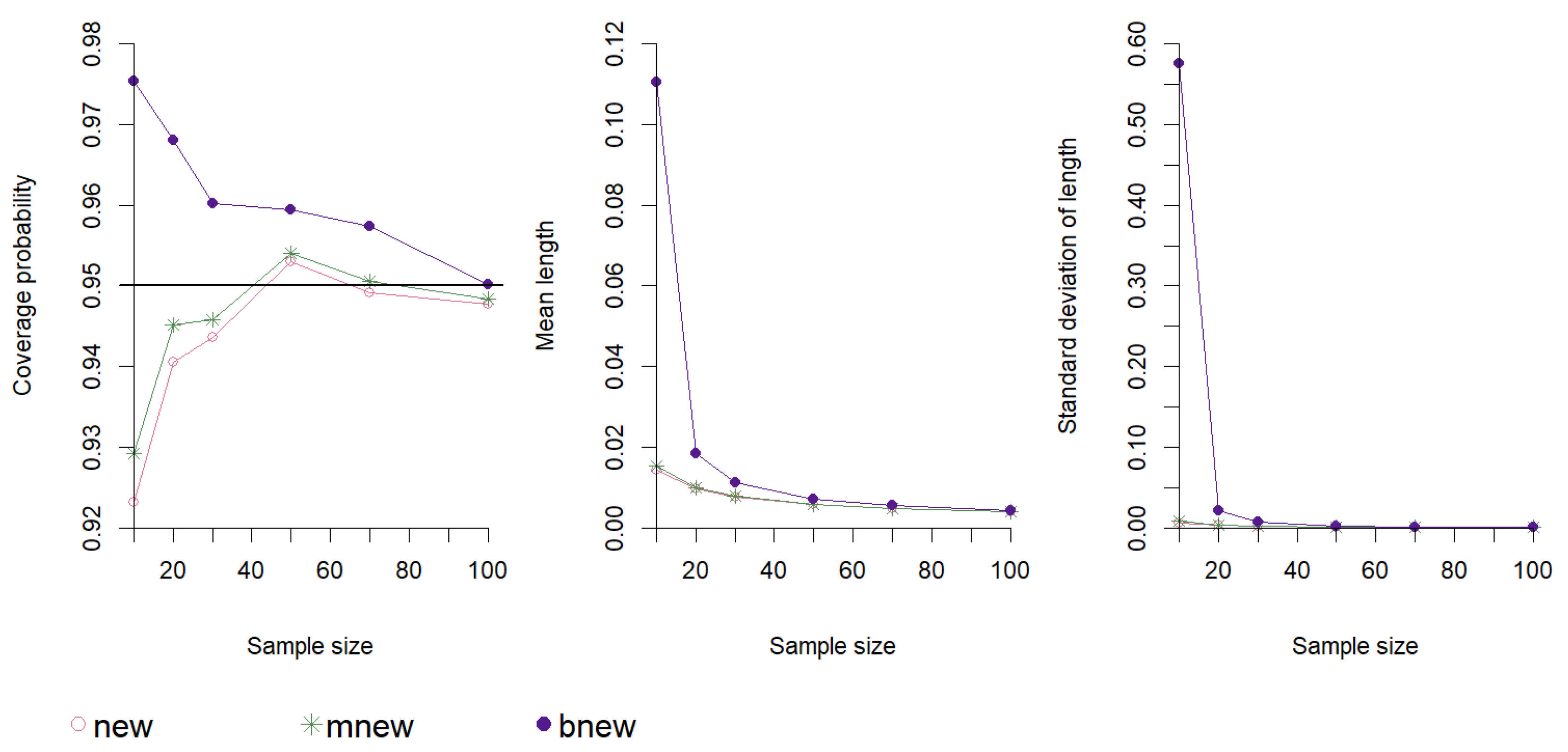
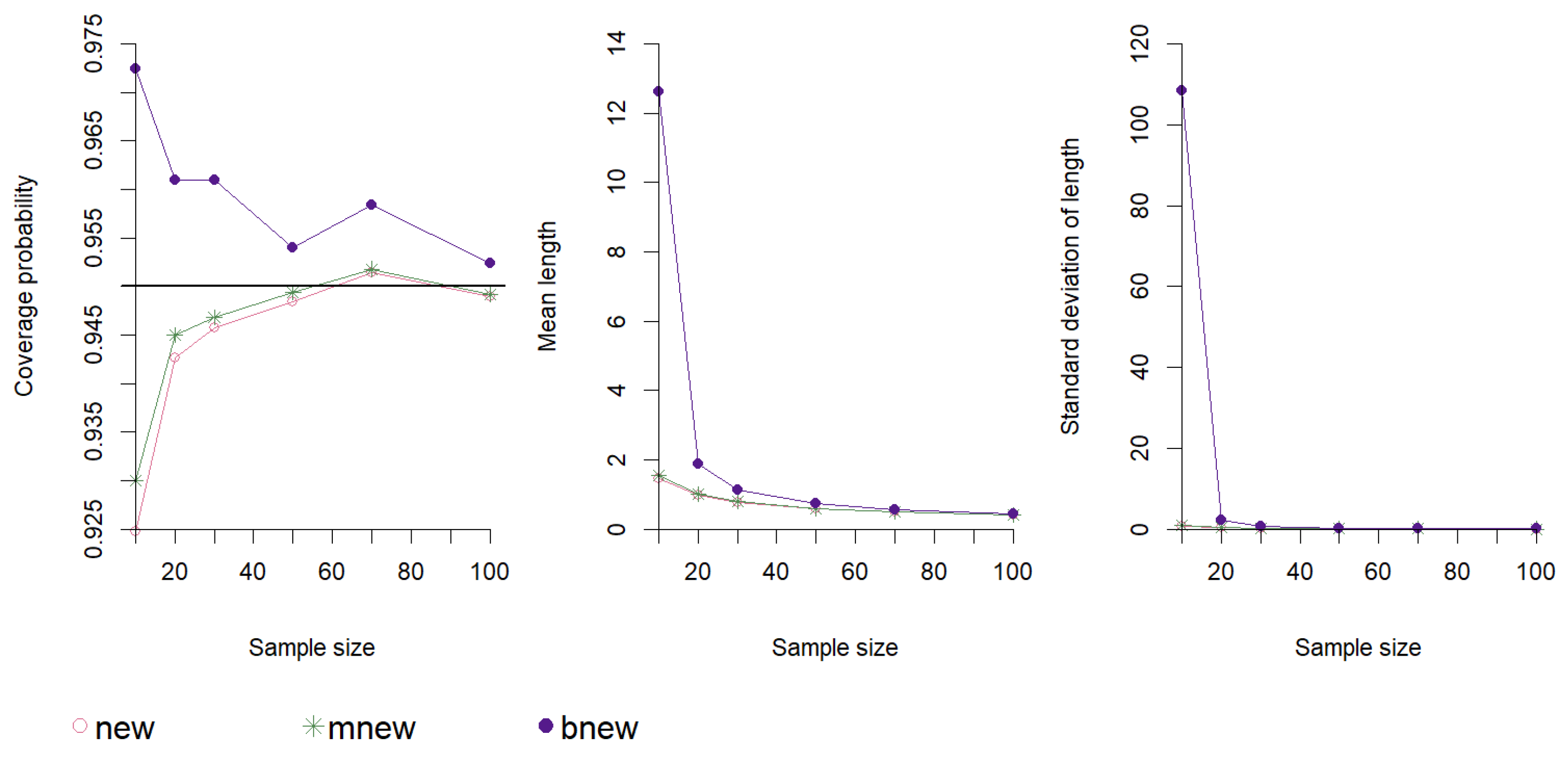
Regarding the newly proposed Edgeworth-based confidence interval, the modified version demonstrates a more pronounced advantage in terms of estimated coverage probability, accompanied by a slightly greater mean and standard deviation of the length. The bootstrap version has a higher estimated coverage probability than the other two for the majority of the sample sizes, but with a higher mean and standard deviation of the length, especially for the sample sizes n = 10 and n = 20 (see example Figure 3 and Figure 4).
The modified versions of the Edgeworth-based confidence intervals offers some improvement in the coverage probability and should be taken into account over the non-modified version. We included modified and bootstrap versions of the Edgeworth-based confidence intervals in the overall comparison of the performance of different interval estimators.

5.2. Overall Comparison of the Confidence Intervals

We summarized the results of the simulation study in Table 1 and Table 2. Normal distribution managed to attain the nominal coverage probability only for sample size n = 100 from normal distribution (with an estimated coverage probability equal to 95.08 % ). We did not include the results of the normal confidence interval in the presented tables due to the interval’s inferior performance.
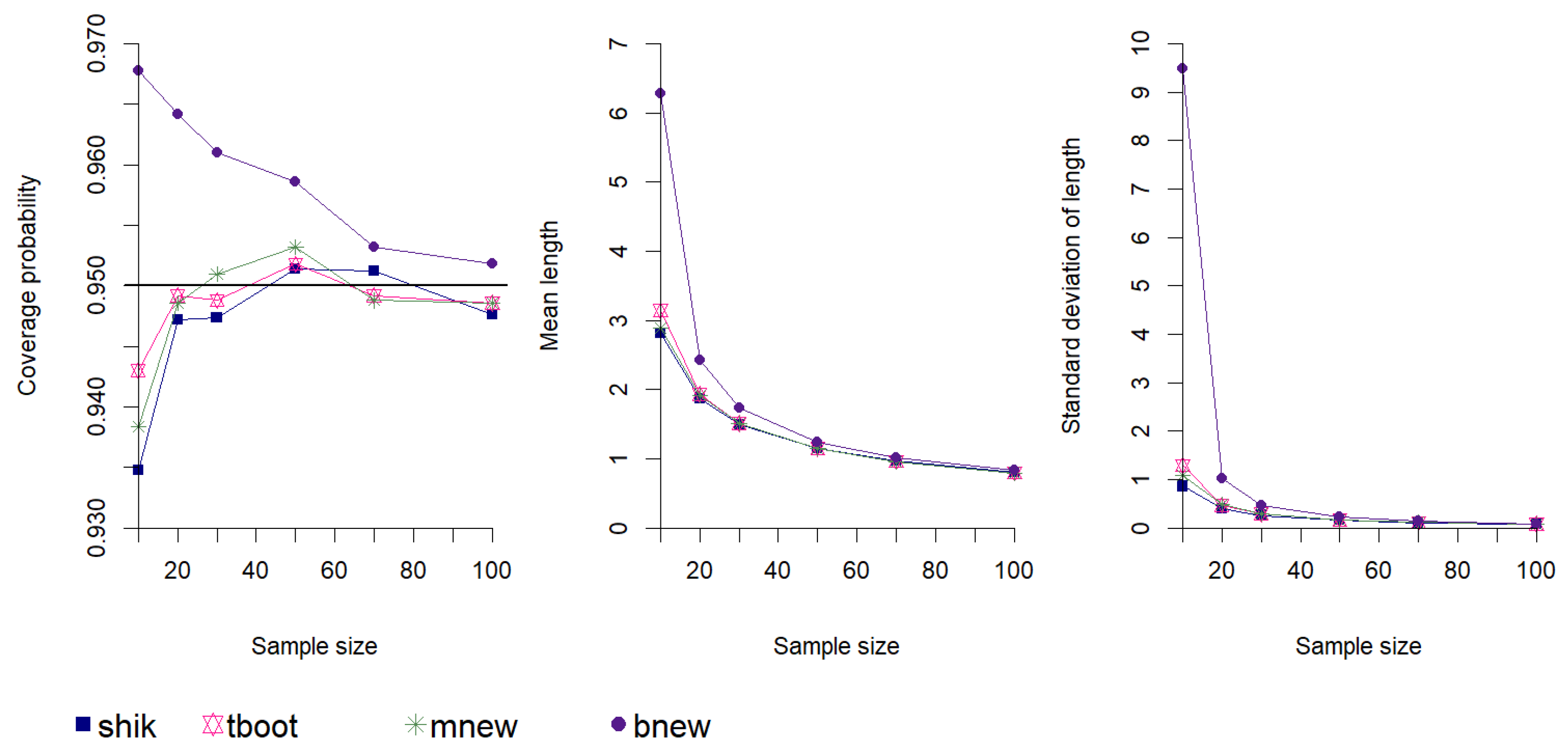
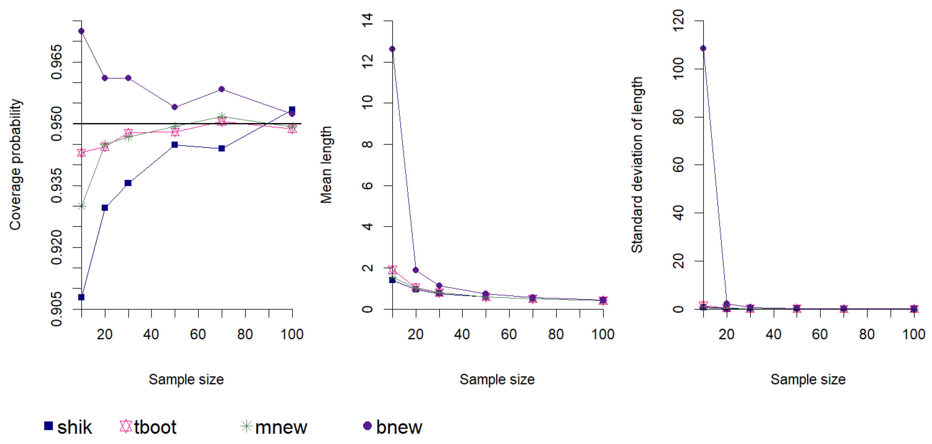
We further compared the confidence intervals by graphically representing the values of three key metrics (estimated coverage probability, mean, and standard deviation of the interval length) on line graphs for each of the considered distributions. In the graphical comparisons, we included only the interval estimators that attained nominal coverage probability for at least one sample size. Examples of the graphical comparisons for the random samples from the distribution with both moderate skewness and kurtosis and the distribution with both high skewness and kurtosis are shown in the Figure 5 and Figure 6.
The bootstrap new confidence interval achieved a nominal coverage probability for all positively skewed distributions and all sample sizes. However, for small samples ( n = 10 ), the mean and standard deviation of the length were significantly higher. In the case of small asymmetry, the modified new confidence interval attained nominal coverage probability for the majority of sample sizes. For moderate to high positive skewness, this confidence interval attained a nominal level for at least one sample size with the lowest estimated coverage probability of 92.9 % (beta B ( 1 , 100 ) distribution). Bootstrap t confidence interval was generally ranked third in terms of coverage (the lowest estimated coverage probability equal to 93.7 % for log-normal distribution), and Shi-Kibria’s t confidence interval was ranked fourth (with the lowest value of estimated coverage probability 90.78 % for exponential distribution). Other t confidence intervals failed to achieve the nominal coverage probability for moderate to highly skewed distributions, with the exception of larger samples from the log-normal distribution. Their performance was better in the cases of small skewness. Modified Hall’s confidence interval underperformed in all cases, except for the large samples from distributions with small asymmetry. Bootstrap Hall’s confidence interval had slightly better performance.
As expected, similar performance of the first four ranked methods is observed for negatively skewed distributions, with slightly worse performance of the t and bootstrap t confidence intervals for beta B ( 10 , 1 ) distribution than their positively skewed counterparts (see Table A1 in the Appendix A).
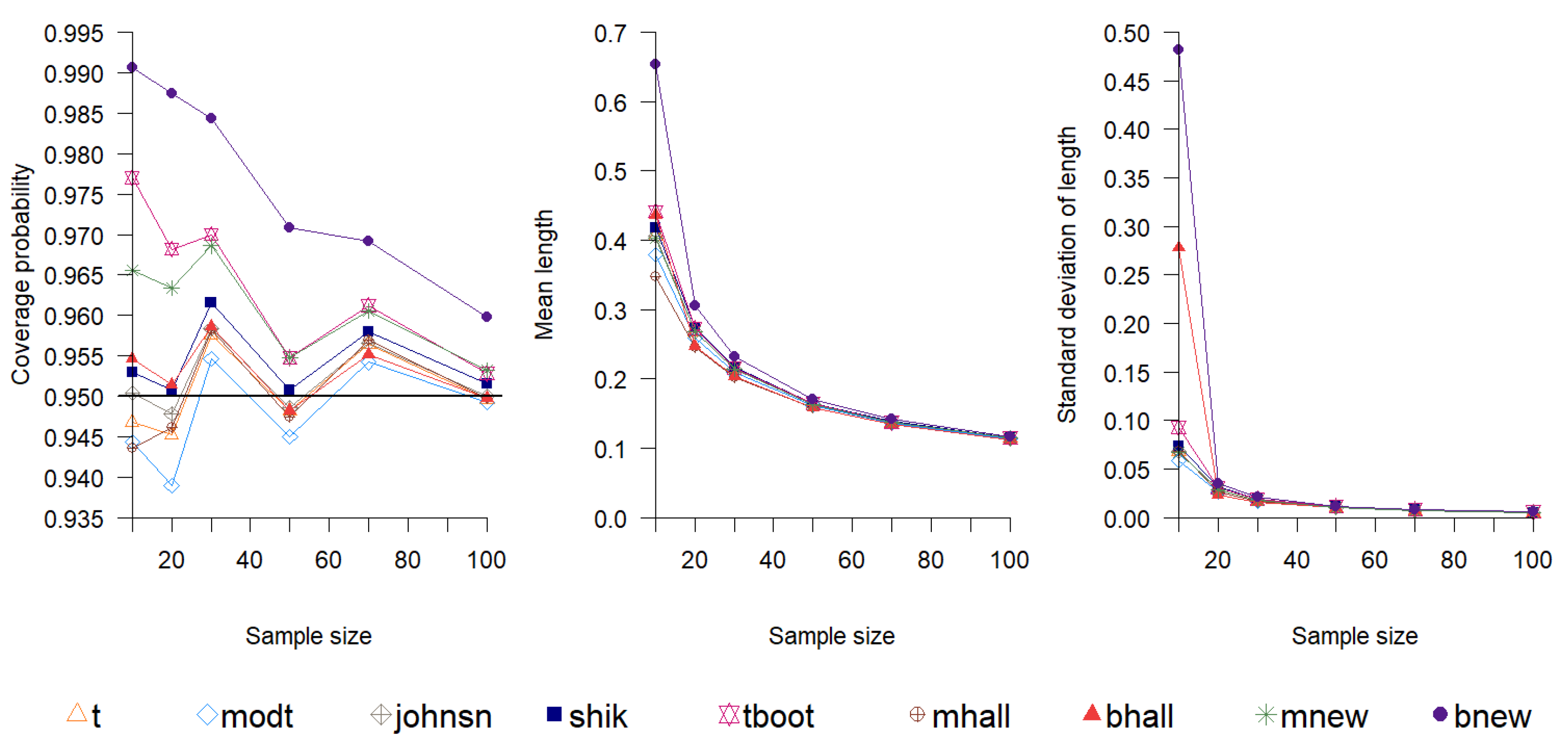
For symmetric distributions, bootstrap new confidence intervals attained nominal coverage probability for all sample sizes. One exception is the logistic distribution, which has a higher peak and heavier tails than a normal distribution with the same variance ( k = 1.2 ). In this case, the proposed bootstrap confidence interval fell below 95 % for sample sizes n = 30 and n = 100 , but with very little deviation (the lowest estimated coverage probability was 94.78 % ). Shi-Kibria’s t confidence interval achieved a nominal coverage probability for all sample sizes from the logistic distribution and for most sample sizes from other symmetric distributions. Johnson’s confidence interval ranked third in terms of coverage, except in the case of uniform distribution ( k = 1.2 ), where its performance was behind the bootstrap t and modified new confidence intervals. The new modified confidence interval reached the nominal coverage probability for the majority of the sample sizes, except for the logistic distribution, where it managed to attain 95 % for only one sample size (the lowest estimated coverage probability was 94.54 % ). The coverage of the bootstrap t confidence interval was poorer, whereas the other t and Hall’s confidence intervals showed better coverage compared to skewed distributions. An example of the graphical comparisons of the confidence intervals for the random samples from the uniform distribution is shown in Figure 7.
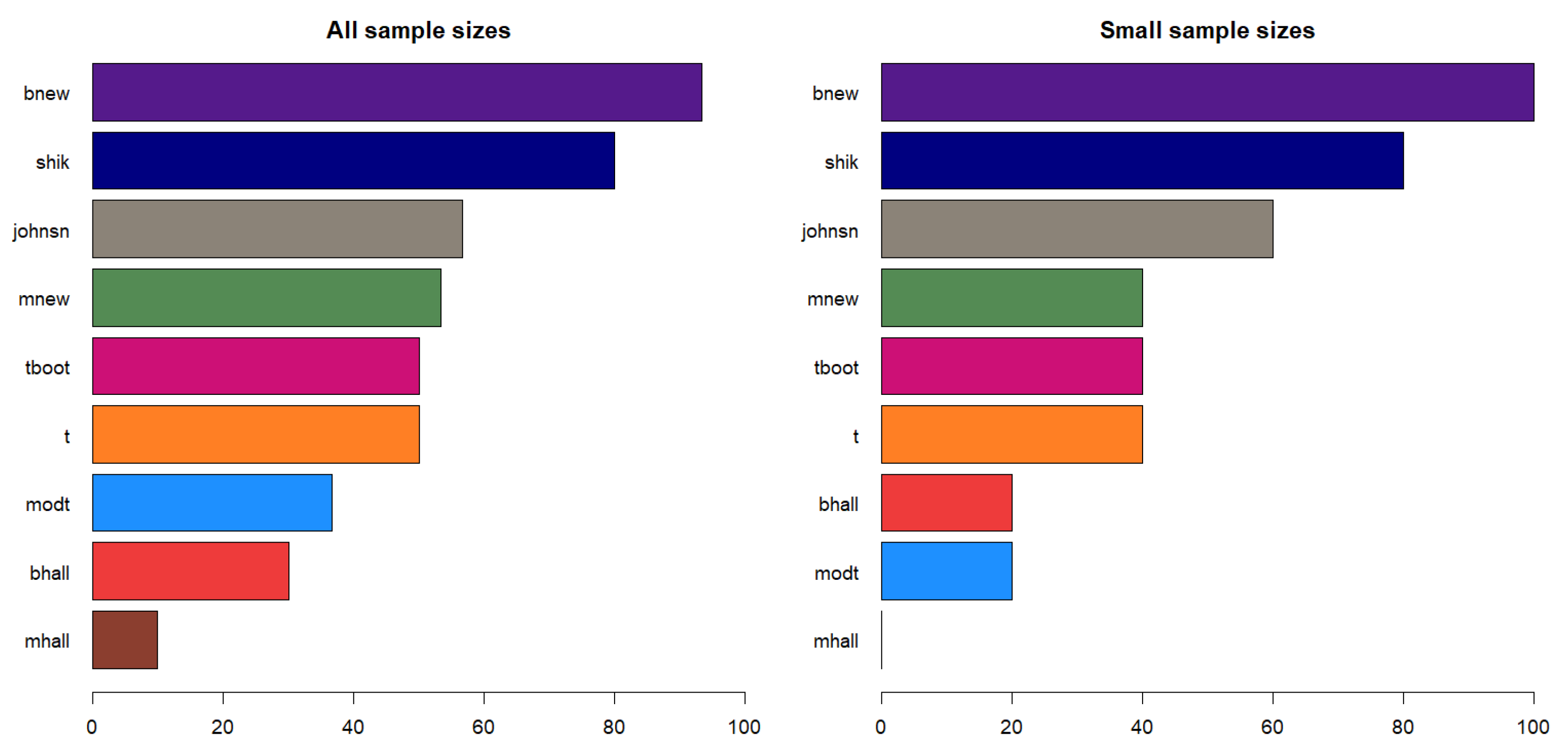
We displayed a simple summary of the confidence intervals’ performance in terms of coverage probability on the horizontal barplot. For each confidence interval, we counted how many times the estimated coverage probability was at least the nominal coverage probability. We repeated the procedure for symmetric and skewed distributions, taking into account all sample sizes or only small samples ( n = 10 and n = 20 ). Figure 8 represents a barplot of the confidence intervals’ percentages of success for skewed distributions.
The proposed bootstrap confidence interval had a percentage of success of 100 % for all sample sizes and also for small samples from skewed distributions. For all sample sizes, it was followed by a modified new confidence interval with a percentage of success of 50 % , then by the bootstrap t confidence interval with 45 % , and by Shi-Kibria’s t confidence interval with 36.7 % . In this group of four best-ranked methods, Shi-Kibria’s t confidence interval had the shortest mean length for 51.4 % samples, the modified new confidence interval for 34.7 % , and the bootstrap t confidence interval for 13.9 % . In small samples, the bootstrap t confidence interval had the second highest percentage of success ( 30 % ), followed by the modified new confidence interval ( 20 % ) and Shi-Kibria’s t confidence interval ( 15 % ). Comparing four best-ranked methods, Shi-Kibria’s t confidence interval had the shortest mean length for 70 % of the sample sizes and the modified new confidence interval for 30 % of them.
Figure 9 represents a barplot of the confidence intervals’ percentages of success for symmetric distributions.
The proposed bootstrap confidence interval had a percentage of success of 93.3 % for all sample sizes from symmetric distributions. It was followed by Shi-Kibria’s t confidence interval with a percentage of success of 80 % , then by Johnson’s t confidence interval with 56.7 % , and by the modified new confidence interval with 53.3 % . In this group of four best-ranked methods, Johnson’s t confidence interval had the shortest mean length for 82.8 % samples, the modified new confidence interval for 16.1 % , and the Shi-Kibria’s t confidence interval for 1.1 % . In small samples, the bootstrap new confidence interval had the highest percentage of success ( 100 % ), followed by Shi-Kibria’s ( 80 % ) and Johnson’s t ( 60 % ) confidence intervals, and modified new confidence interval ( 40 % ). Comparing four best-ranked methods, Johnson’s t confidence interval had the shortest mean length for 85 % of the sample sizes and the modified new confidence interval for 15 % of them.

6. Discussion

The proposed bootstrap Edgeworth-based confidence interval demonstrated superior coverage probability for both small and large random samples from diverse symmetric and skewed distributions. This confidence interval managed to attain nominal coverage probability for all considered distributions and all sample sizes, except for some medium-sized samples from symmetric logistic distribution, with the lowest estimated coverage probability of 94.78 % . However, the mean and standard deviation of the interval lengths were the highest of all the confidence intervals, with large values for small samples ( n = 10 ). Bootstrap t confidence interval is reported in the literature to produce long intervals for small samples [13,28]. A large standard deviation of the length shows that bootstrap confidence intervals produce both short and long intervals for small samples (i.e., the length is not consistently long). Approximation of the distribution of the test statistics can be poorer for small samples, as these samples provide much less information about the values of the variable of interest.
In the cases of no or small skewness, the modified new Edgeworth-based confidence interval achieved nominal coverage probability for at least half of the sample sizes. For moderate to high skewness, this confidence interval achieved 95 % for at least one sample size with the lowest estimated coverage probability of 92.9 % . The mean and standard deviation of its length are smaller than for the proposed bootstrap confidence interval. However, overall results show that the bootstrap distribution of the statistic T is much closer to the exact distribution than the Edgeworth expansion with the normal distribution as the baseline. The difference between these two methods is most apparent for small samples, where the modified new confidence interval manages to achieve nominal probability in only 40 % samples from symmetric distributions and 20 % samples from skewed distributions.
Johnson’s and Shi-Kibria’s t confidence intervals attain nominal coverage probability for a majority of samples from symmetric distributions. However, their performance is not satisfactory enough in skewed distributions, achieving 95 % only occasionally and with the lowest estimated coverage probability around 90 % . Bootstrap t confidence interval managed to achieve the nominal coverage probability for half of the samples from symmetric distributions and 45 % of the samples from skewed distributions. Normal, Hall’s modified, and Hall’s bootstrap confidence intervals underperformed by achieving nominal coverage probability for only one (normal) or just a few sample sizes (Hall) in total.

7. Conclusions

Previous research showed that finding an interval estimator for the population mean that performs well in the cases of highly skewed distributions poses a real challenge [17]. We have analyzed four types of confidence intervals for the population mean: normal confidence interval, t confidence intervals, bootstrap t confidence interval and confidence intervals based on Edgeworth expansion. The exact or approximate distribution of the statistic T = X ¯ μ S E M ^ is used for the construction of these confidence intervals. We proposed a new confidence interval for the population mean, which is based on the Edgeworth expansion of the second order of the distribution of the statistic T. This expansion corrects the normal approximation by incorporating information about the skewness and kurtosis of the population distribution. We have created two additional versions of the proposed interval estimator. The modified version includes the bias-corrected estimates of the skewness and kurtosis, while the bootstrap version uses the bootstrap distribution of the statistic T as the baseline.
We conducted a simulation study to compare various interval estimators by generating random samples of different sizes from symmetric and skewed distributions with varying levels of kurtosis. We measured the performance using the coverage probability, mean, and standard deviation of the interval length. The overall comparison of the confidence intervals included the modified versions of the Edgeworth-based confidence intervals, which had a slight advantage over the non-modified ones.
The proposed bootstrap confidence interval achieved a nominal coverage probability for all sample sizes from both symmetric and skewed distributions. One exception is the heavy-tailed logistic distribution, where the proposed bootstrap confidence interval fell below 95 % for some samples but with very little deviation (the lowest estimated coverage probability was 94.78 % ). However, the main drawbacks of this method are the high values of the mean and standard deviation for small samples ( n = 10 ). A large standard deviation of the length shows that the proposed bootstrap method produces intervals of both small and large length.
For symmetric or lightly skewed distributions, the proposed modified Edgeworth-based confidence interval achieved nominal coverage probability for the majority of sample sizes. For moderate to high positive skewness, this confidence interval attained 95 % for at least one sample size with the lowest estimated coverage probability of 92.9 % . In skewed distributions, bootstrap t confidence interval was generally ranked third in terms of coverage (the lowest estimated coverage probability of 93.7 % ), and Shi-Kibria’s t confidence interval was ranked fourth (with the lowest value of estimated coverage probability of 90.78 % ). These three methods generally provide shorter intervals than the proposed bootstrap confidence interval, but their overall coverage is not at the satisfactory level. For all sample sizes, the second-ranked modified new confidence interval achieves the nominal coverage probability in 50 % of the samples. In small samples, the difference between the first and second-ranked methods is even more drastic. The second-ranked bootstrap t confidence interval manages to attain 95 % in only 30 % samples. The percentage of success is even lower for other confidence intervals when considering all or only small samples. For symmetric distributions, the situation improves in terms of identifying a method with adequate coverage and a shorter interval length. Shi-Kibria’s confidence interval has a percentage of success of 80 % when considering both all sample sizes or only small samples.
The new bootstrap Edgeworth-based confidence interval for the population mean can be recommended for use in general practice for both symmetric and skewed distributions based on its superior coverage performance. If a researcher is concerned with the length of the confidence interval for samples up to size 20, we can make the following recommendations. For a small sample from symmetric distribution, we can recommend Shi-Kibria’s confidence interval. If the small sample comes from a skewed distribution, we cannot recommend any of the other confidence intervals, as they do not provide satisfactory coverage.
In our future work, we plan to focus on developing a modified version of our bootstrap Edgeworth-based confidence interval for the population mean, which will have both excellent coverage and a shorter mean length.

Funding

This research received no external funding.

Data Availability Statement

Data available on request from the author.

Conflicts of Interest

The author declares no conflicts of interest.

Appendix A

Table A1. Confidence intervals’ coverage, mean length and standard deviation of length for negatively skewed distributions.
nEstimated Coverage ProbabilityMean Length (Standard Deviation)
tmodtjohnsnshiktbootmhallbhallmnewbnewtmodtjohnsnshiktbootmhallbhallmnewbnew
beta B ( 2 , 1 ) ( γ = 0.57 , k = 0.6 )
100.940.93360.94080.9440.9620.93240.9450.95120.98220.33070.31560.33070.34150.37250.30710.42010.33760.6509
(0.0691)(0.0655)(0.0691)(0.0743)(0.1065)(0.1058)(0.2984)(0.0744)(0.8186)
200.94940.94620.95060.95220.96440.94980.95460.96060.98420.21830.2140.21830.22420.22520.2040.2120.22130.2624
(0.0308)(0.0292)(0.0308)(0.0335)(0.0331)(0.0304)(0.0458)(0.0312)(0.0468)
300.950.9480.9520.95520.96220.9490.95280.9610.97680.17520.1730.17520.17930.17810.1670.1690.1770.1952
(0.0195)(0.0187)(0.0195)(0.0212)(0.0204)(0.0185)(0.0178)(0.0196)(0.0235)
500.94740.94580.94860.95080.95520.94620.94560.95480.96780.13340.13240.13340.1360.13450.12950.13020.13420.1415
(0.0114)(0.0111)(0.0114)(0.0123)(0.0118)(0.011)(0.0109)(0.0114)(0.0126)
700.9420.94160.94240.94560.95040.94480.94480.95020.96180.1120.11140.1120.1140.11260.10970.110.11250.1166
(0.0081)(0.0079)(0.0081)(0.0088)(0.0085)(0.0079)(0.008)(0.0081)(0.0089)
1000.95160.95140.95220.95560.95620.9530.95320.95660.96440.09330.0930.09330.09490.09370.0920.09220.09360.096
(0.0056)(0.0055)(0.0056)(0.0061)(0.006)(0.0055)(0.0058)(0.0056)(0.0062)
beta B ( 10 , 1 ) ( γ = 1.52 , k = 2.78 )
100.91060.90480.91440.92060.94860.9040.92380.93760.97660.11210.11380.11210.11780.14780.13210.20440.12640.5854
(0.0392)(0.0455)(0.0392)(0.0427)(0.0867)(0.0805)(0.1596)(0.0562)(2.3048)
200.9230.92780.92560.93020.94640.92680.93640.94580.96560.07540.07830.07540.07890.08480.08610.10770.08250.1276
(0.0185)(0.0217)(0.0185)(0.0202)(0.0265)(0.0416)(0.0741)(0.0244)(0.0944)
300.93560.93920.93720.94260.95020.93860.94160.95060.96320.06080.06290.06080.06350.06540.06560.07290.0650.0828
(0.0123)(0.0141)(0.0123)(0.0135)(0.0153)(0.0251)(0.0391)(0.0152)(0.031)
500.94380.94720.94420.94980.9470.93880.9430.94740.95620.04670.04780.04670.04870.04870.04780.04940.04870.0554
(0.0073)(0.008)(0.0073)(0.008)(0.0084)(0.0106)(0.014)(0.0083)(0.0122)
700.94040.94440.94280.94940.9510.94540.94920.95260.96040.03930.04010.03930.0410.04050.03960.04020.04050.0442
(0.0052)(0.0055)(0.0052)(0.0057)(0.0057)(0.0058)(0.0064)(0.0057)(0.0073)
1000.94660.94860.94640.9530.94760.94640.9460.95040.95280.03270.03320.03270.03410.03340.03280.03310.03340.0355
(0.0035)(0.0037)(0.0035)(0.0039)(0.0038)(0.0037)(0.0039)(0.0038)(0.0045)
beta B ( 100 , 1 ) ( γ = 1.94 , k = 5.54 )
100.90180.90220.90540.90840.94240.9050.9220.93060.9750.0130.01350.0130.01370.01810.0160.02490.01520.0936
(0.0053)(0.0065)(0.0053)(0.0058)(0.0128)(0.0106)(0.0199)(0.0082)(0.402)
200.91920.92460.92120.9270.94840.92720.93640.94580.9670.00880.00940.00880.00920.01030.0110.01410.010.018
(0.0026)(0.0033)(0.0026)(0.0028)(0.0041)(0.0064)(0.0102)(0.0039)(0.0184)
300.92860.93640.93060.93540.95040.93680.94160.94820.96060.00710.00750.00710.00740.00790.00830.00970.00780.0109
(0.0017)(0.0021)(0.0017)(0.0019)(0.0024)(0.0042)(0.0065)(0.0024)(0.0072)
500.93540.94120.93740.9440.94940.93980.94480.94880.95480.00550.00570.00550.00570.00580.0060.00640.00590.007
(0.001)(0.0012)(0.001)(0.0011)(0.0013)(0.0023)(0.0032)(0.0013)(0.0024)
700.94180.9460.94180.94920.94760.94360.94480.95020.95540.00460.00480.00460.00480.00480.00490.00510.00490.0055
(0.0007)(0.0009)(0.0007)(0.0008)(0.0009)(0.0014)(0.0019)(0.0009)(0.0015)
1000.94160.94560.94160.95140.9490.94560.94760.94980.95280.00390.0040.00390.0040.0040.0040.0040.0040.0044
(0.0005)(0.0006)(0.0005)(0.0006)(0.0006)(0.0008)(0.001)(0.0006)(0.0008)
t—standard t confidence interval, modt—modified t confidence interval, johnsn—Johnson’s t confidence interval, shik—Shi-Kibria’s t confidence interval), tboot—bootstrap t-confidence interval, mhall—modified Hall’s confidence interval, bhall—bootstrap Hall’s confidence interval, mnew—modified new confidence interval, bnew—bootstrap new confidence interval.

References

  1. Thompson, S.G.; Barber, J.A. How should cost data in pragmatic randomised trials be analysed? BMJ 2000, 320, 1197–1200. [Google Scholar] [CrossRef] [PubMed]
  2. Klugman, S.A.; Panjer, H.H.; Willmot, G.E. Loss Models: From Data to Decisions, 5th ed.; Wiley: New York, NY, USA, 2019. [Google Scholar]
  3. Holmes, M.; Maser, K. Using Median Expenditures: Impact on Household Spending Data; Household Expenditures Research Paper Series; Statistics Canada: Ottawa, ON, Canada, 2003. [Google Scholar]
  4. Blanca, M.J.; Arnau, J.; López-Montiel, D.; Bono, R.; Bendayan, R. Skewness and kurtosis in real data samples. Methodol. Eur. J. Res. Methods Behav. Soc. Sci. 2013, 9, 78–84. [Google Scholar] [CrossRef]
  5. Indrayan, A.; Mishra, A. The importance of small samples in medical research. J. Postgrad. Med. 2021, 67, 219–223. [Google Scholar] [CrossRef] [PubMed]
  6. Johnson, N.J. Modified t-tests and confidence intervals for asymmetrical population. J. Am. Stat. Assoc. 1978, 73, 536–544. [Google Scholar] [CrossRef]
  7. Willink, R. A confidence interval and test for the mean of an asymmetric distribution. Commun. Stat. Methods 2005, 34, 753–766. [Google Scholar] [CrossRef]
  8. Shi, W.; Kibria, B.M.G. On some confidence intervals for estimating the mean of a skewed population. Int. J. Math. Educ. Sci. Technol. 2007, 38, 412–421. [Google Scholar] [CrossRef]
  9. Abu-Shawiesh, M.O.A.; Banik, B.; Kibria, B.M.G. Confidence Intervals based on absolute deviation for population mean of a positively skewed distribution. Int. J. Comput. Theor. Stat. 2018, 5, 1–13. [Google Scholar] [CrossRef] [PubMed]
  10. Abu-Shawiesh, M.O.A.; Saghir, A. Robust confidence intervals for the population mean alternatives to the Student-t confidence interval. J. Mod. Appl. Stat. Methods 2019, 18, eP2721. [Google Scholar] [CrossRef]
  11. O’Neill, B. Some Useful Moment Results in Sampling Problems. Am. Stat. 2014, 68, 282–296. [Google Scholar] [CrossRef]
  12. Efron, B. Nonparametric Standard Errors and Confidence Intervals. Can. J. Stat. 1981, 2, 139–158. [Google Scholar] [CrossRef]
  13. Di Ciccio, T.J.; Efron, B. Bootstrap Confidence Intervals. Stat. Sci. 1996, 11, 189–228. [Google Scholar]
  14. Hall, P. On the removal of skewness by transformation. J. R. Stat. Soc. Ser. 1992, 54, 221–228. [Google Scholar] [CrossRef]
  15. Zhou, X.H.; Dinh, P. Nonparametric confidence intervals for the one- and two-sample problems. Biostatistics 2005, 6, 187–200. [Google Scholar] [CrossRef] [PubMed]
  16. Zhou, X.-H.; Gao, S. One–sided confidence intervals for means of positively skewed distribution. Am. Stat. 2000, 54, 100–104. [Google Scholar] [CrossRef]
  17. Banik, S.; Kibria, B.M.G. Comparison of Some Parametric and Nonparametric Type One Sample Confidence Intervals for Estimating the Mean of a Positively Skewed Distribution. Commun. Stat. Simul. Comput. 2010, 39, 361–389. [Google Scholar] [CrossRef]
  18. DeCarlo, L.T. On the Meaning and Use of Kurtosis. Psychol. Methods 1997, 2, 292–307. [Google Scholar] [CrossRef]
  19. Neyman, J. Outline of a Theory of Statistical Estimation Based on the Classical Theory of Probability. Philos. Trans. R. Soc. 1937, 236, 333–380. [Google Scholar]
  20. Wasserman, L. All of Statistics: A Concise Course in Statistical Inference; Springer Texts in Statistics: New York, NY, USA, 2004; p. 75. [Google Scholar]
  21. Wilcox, R. Introduction to Robust Estimation and Hypothesis Testing, 3rd ed.; Academic Press: New York, NY, USA, 2012. [Google Scholar]
  22. Hall, P. The Bootstrap and Edgeworth Expansion; Springer: New York, NY, USA, 1992. [Google Scholar]
  23. Joanes, D.N.; Gill, C.A. Comparing Measures of Sample Skewness and Kurtosis. J. R. Stat. Soc. Ser. 1998, 47, 183–189. [Google Scholar] [CrossRef]
  24. Efron, B.; Tibshirani, R.; Tibshirani, R.J. An Introduction to the Bootstrap; Chapman & Hall/CRC Monographs on Statistics and Applied Probability: Philadelphia, PA, USA, 1994; pp. 124–125. [Google Scholar]
  25. Johnson, N.L.; Kotz, S.; Balakrishnan, N. Continuous Univariate Distributions, 2nd ed.; Wiley-Interscience: New York, NY, USA, 1994; Volume 1. [Google Scholar]
  26. Johnson, N.L.; Kotz, S.; Balakrishnan, N. Continuous Univariate Distributions; Wiley-Interscience: New York, NY, USA, 1995; Volume 2. [Google Scholar]
  27. Piovesana, A.; Senior, G. How Small Is Big: Sample Size and Skewness. Assessment 2018, 25, 793–800. [Google Scholar] [CrossRef] [PubMed]
  28. Davison, A.C.; Hinkley, D.V. Bootstrap Methods and Their Application; Cambridge University Press: Cambridge, UK, 1997. [Google Scholar]
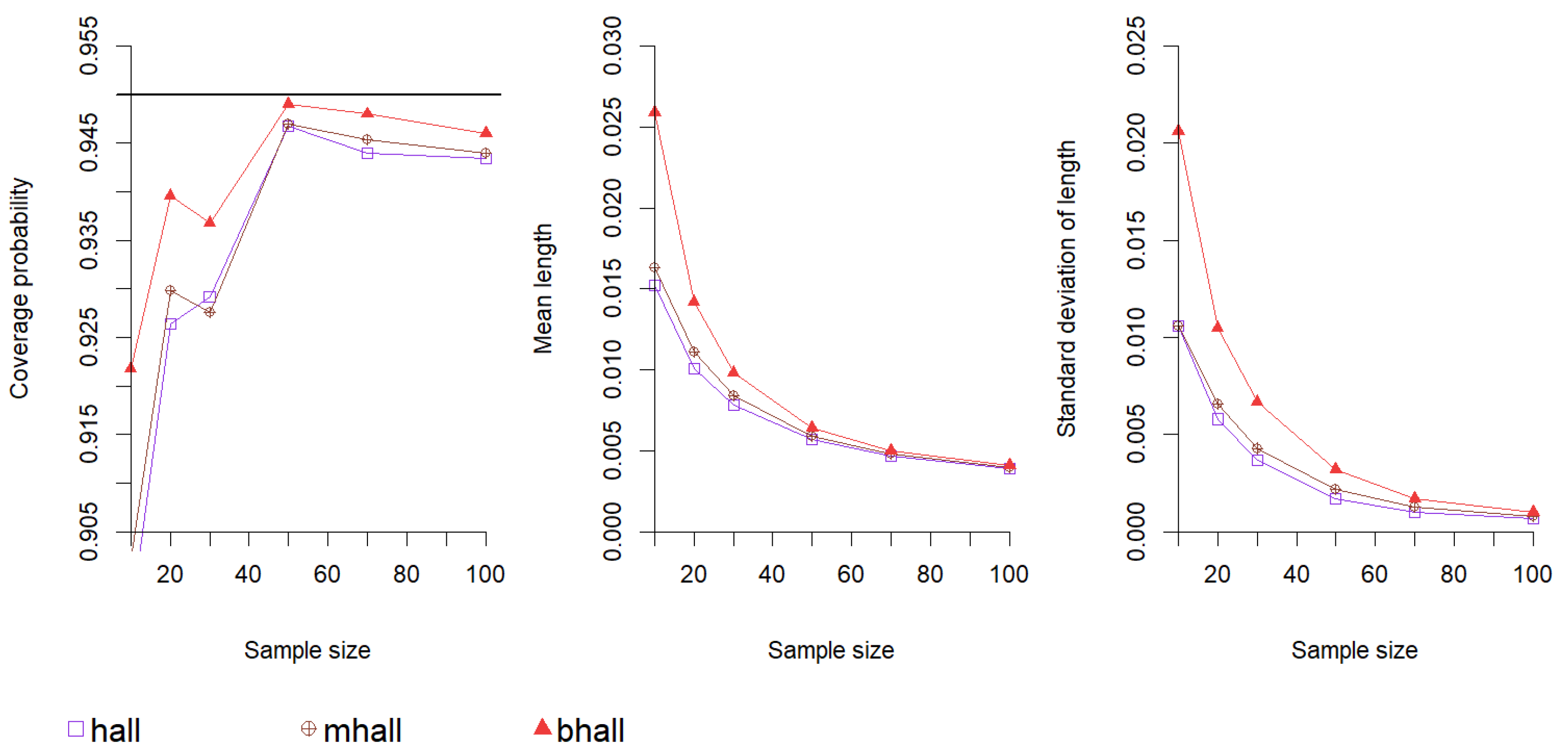
Figure 1. The comparison of the performance of three versions of Hall’s confidence intervals for samples from the beta distribution B ( 1 , 100 ) with skewness γ = 1.94 and excess kurtosis k = 5.54 . Abbreviations: hall-Hall’s confidence interval, mhall-modified Hall’s confidence interval, bhall-bootstrap Hall’s confidence interval.
Symmetry 16 01424 g001
Figure 2. The comparison of the performance of three versions of Hall’s confidence interval for samples from the gamma distribution G ( 1 , 1 ) with skewness γ = 2 and excess kurtosis k = 6 . Abbreviations: hall-Hall’s confidence interval, mhall-modified Hall’s confidence interval, bhall-bootstrap Hall’s confidence interval.
Symmetry 16 01424 g002
Figure 3. The comparison of the performance of three versions of the new confidence interval for samples from the beta distribution B ( 1 , 100 ) with skewness γ = 1.94 and excess kurtosis k = 5.54 . Abbreviations: new-new confidence interval, mnew-modified new confidence interval, bnew-bootstrap new confidence interval.
Symmetry 16 01424 g003
Figure 4. The comparison of the performance of three versions of the new confidence interval for samples from the gamma distribution G ( 1 , 1 ) with skewness γ = 2 and excess kurtosis k = 6 . Abbreviations: new-new confidence interval, mnew-modified new confidence interval, bnew-bootstrap new confidence interval.
Symmetry 16 01424 g004
Figure 5. The comparison of the performance of interval estimators that achieved nominal coverage probability for at least one sample size for random samples from gamma G ( 4 , 1 ) distribution ( γ = 1 , k = 1.5 ). Abbreviations: shik—Shi- Kibria’s t confidence interval, tboot—bootstrap t confidence interval, mnew—modified new confidence interval, bnew—bootstrap new confidence interval.
Symmetry 16 01424 g005
Figure 6. The comparison of the performance of interval estimators that achieved nominal coverage probability for at least one sample size for random samples from gamma G ( 1 , 1 ) distribution ( γ = 2 , k = 6 ). Abbreviations: shik—Shi- Kibria’s t confidence interval, tboot—bootstrap t confidence interval, mnew—modified new confidence interval, bnew—bootstrap new confidence interval.
Symmetry 16 01424 g006
Figure 7. The comparison of the performance of interval estimators that achieved nominal coverage probability for at least one sample size for random samples from beta B ( 1 , 1 ) (standard uniform) distribution ( γ = 0 , k = 1.2 ). Abbreviations: t—standard t confidence interval, modt—modified t confidence interval, johnsn—Johnson’s t confidence interval, shik—Shi-Kibria’s t confidence interval), tboot—bootstrap t-confidence interval, mhall—modified Hall’s confidence interval, bhall—bootstrap Hall’s confidence interval, mnew—modified new confidence interval, bnew—bootstrap new confidence interval.
Symmetry 16 01424 g007
Figure 8. The comparison of the confidence intervals’ performance in terms of coverage probability for skewed distributions. Abbreviations: t—standard t confidence interval, modt—modified t confidence interval, johnsn—Johnson’s t confidence interval, shik—Shi-Kibria’s t confidence interval), tboot—bootstrap t-confidence interval, mhall—modified Hall’s confidence interval, bhall—bootstrap Hall’s confidence interval, mnew—modified new confidence interval, bnew—bootstrap new confidence interval.
Symmetry 16 01424 g008
Figure 9. The comparison of the confidence intervals’ performance in terms of coverage probability for symmetric distributions. Abbreviations: t—standard t confidence interval, modt—modified t confidence interval, johnsn—Johnson’s t confidence interval, shik—Shi-Kibria’s t confidence interval), tboot—bootstrap t-confidence interval, mhall—modified Hall’s confidence interval, bhall—bootstrap Hall’s confidence interval, mnew—modified new confidence interval, bnew—bootstrap new confidence interval.
Symmetry 16 01424 g009
Table 1. Confidence intervals’ coverage, mean length, and standard deviation of length for positively skewed distributions.
nEstimated Coverage ProbabilityMean Length (Standard Deviation)
tmodtjohnsnshiktbootmhallbhallmnewbnewtmodtjohnsnshiktbootmhallbhallmnewbnew
beta B ( 1 , 2 ) ( γ = 0.57 , k = 0.6 )
100.93860.93140.94060.94360.96240.92620.94160.94980.9880.33090.31510.33090.34180.37420.30360.42920.33690.6677
(0.0703)(0.0659)(0.0703)(0.0757)(0.1129)(0.0988)(0.3202)(0.0744)(0.9364)
200.94360.94120.94640.94940.96160.94440.94960.9590.97960.21870.21420.21870.22450.22560.20410.21220.22160.2629
(0.0307)(0.0291)(0.0307)(0.0334)(0.033)(0.0296)(0.0439)(0.0309)(0.0522)
300.94560.94460.94760.95080.95860.94580.9470.95680.97220.17530.17310.17530.17940.17840.16710.16910.1770.1956
(0.02)(0.0192)(0.02)(0.0216)(0.0209)(0.0189)(0.0183)(0.0201)(0.0241)
500.94420.94340.9470.95020.95620.94680.9490.95540.96580.13330.13240.13330.1360.13450.12960.13030.13420.1417
(0.0115)(0.0112)(0.0115)(0.0125)(0.012)(0.0111)(0.0111)(0.0115)(0.0128)
700.94640.9460.94740.95140.95380.94920.94680.95580.96180.11210.11150.11210.11420.11270.10980.11020.11260.1169
(0.0081)(0.008)(0.0081)(0.0088)(0.0085)(0.0079)(0.0081)(0.0082)(0.0089)
1000.95080.95040.95180.95440.95520.9510.9510.95560.9630.09340.09310.09340.09510.09380.09210.09230.09380.0962
(0.0056)(0.0055)(0.0056)(0.0061)(0.0061)(0.0055)(0.0058)(0.0056)(0.0063)
beta B ( 1 , 10 ) ( γ = 1.52 , k = 2.78 )
100.91140.9080.91340.91620.94280.9030.92260.93280.9730.11090.11230.11090.11620.14470.12980.20270.12460.5473
(0.0388)(0.0446)(0.0388)(0.0422)(0.081)(0.0779)(0.1583)(0.0549)(2.8423)
200.92620.93040.92760.93380.95280.93260.9430.94960.9690.07530.07810.07530.07880.08470.0860.1070.08240.1279
(0.0186)(0.0219)(0.0186)(0.0203)(0.0264)(0.0421)(0.0733)(0.0249)(0.09)
300.93320.93880.93580.94380.95480.9440.9490.9560.96820.06070.06270.06070.06340.06540.0650.07280.06480.0831
(0.012)(0.0137)(0.012)(0.0131)(0.0152)(0.0235)(0.0389)(0.0149)(0.0325)
500.94180.9450.94240.94880.95380.94860.95220.95440.96320.04660.04780.04660.04860.04870.04760.04930.04870.0555
(0.0071)(0.0078)(0.0071)(0.0077)(0.0081)(0.0099)(0.0133)(0.0081)(0.0119)
700.93940.94460.94120.94820.95040.94440.94880.95040.95420.03920.040.03920.04090.04040.03950.04030.04040.0443
(0.0051)(0.0055)(0.0051)(0.0056)(0.0057)(0.0059)(0.0069)(0.0056)(0.0073)
1000.94160.9450.94260.94920.94760.94280.94380.94740.950.03270.03320.03270.03410.03340.03280.03320.03340.0356
(0.0036)(0.0038)(0.0036)(0.0039)(0.0039)(0.0038)(0.004)(0.0038)(0.0046)
beta B ( 1 , 100 ) ( γ = 1.94 , k = 5.54 )
100.90580.90260.90780.91180.94680.90220.92180.92920.97540.01310.01360.01310.01380.01860.01630.02590.01540.1106
(0.0053)(0.0065)(0.0053)(0.0057)(0.0136)(0.0106)(0.0206)(0.0084)(0.5761)
200.91760.92260.920.9250.9470.92980.93960.94520.9680.00880.00940.00880.00920.01030.01110.01420.010.0184
(0.0026)(0.0034)(0.0026)(0.0028)(0.0042)(0.0066)(0.0105)(0.0039)(0.0217)
300.92420.93240.92720.9340.9470.92760.93680.94580.96020.00710.00750.00710.00750.00790.00840.00980.00790.0112
(0.0017)(0.0022)(0.0017)(0.0019)(0.0025)(0.0043)(0.0067)(0.0025)(0.0077)
500.93840.9440.9390.94660.95220.9470.9490.9540.95940.00550.00570.00550.00570.00580.00590.00640.00590.0071
(0.001)(0.0012)(0.001)(0.0011)(0.0013)(0.0022)(0.0032)(0.0013)(0.0027)
700.9370.9430.93820.94760.94880.94540.9480.95060.95740.00460.00480.00460.00480.00480.00480.0050.00480.0055
(0.0007)(0.0008)(0.0007)(0.0008)(0.0009)(0.0013)(0.0017)(0.0009)(0.0014)
1000.94380.94780.94460.95060.9480.9440.9460.94840.95020.00390.0040.00390.0040.0040.0040.00410.0040.0044
(0.0005)(0.0006)(0.0005)(0.0006)(0.0006)(0.0008)(0.001)(0.0006)(0.0009)
gamma G ( 100 , 0.1 ) ( γ = 0.2 , k = 0.06 )
100.95060.94240.95160.95440.94740.90060.92420.9460.9682139.2332134.4575139.2332142.1655150.1299127.317178.6623140.8266224.3392
(33.8268)(33.7284)(33.8268)(34.751)(40.0917)(48.1457)(121.685)(36.1823)(131.2656)
200.9530.95080.95320.95560.95240.9320.9440.95020.964292.416591.689492.416593.578694.027786.095494.377293.1071106.8596
(15.4694)(15.6693)(15.4694)(15.7801)(16.2467)(16.4159)(26.0686)(15.981)(20.9608)
300.95020.94980.95020.95180.9480.93680.94580.94820.959674.069773.828774.069774.732674.595270.309574.031774.364580.4221
(9.7421)(9.8488)(9.7421)(9.8942)(10.033)(9.3735)(10.7363)(9.8881)(11.297)
500.95120.95040.95060.95240.95120.94360.9510.95140.958856.514256.460456.514256.847356.663854.723356.405956.618659.0601
(5.8096)(5.8405)(5.8096)(5.8882)(6.0061)(5.6589)(6.0662)(5.8546)(6.3869)
700.95180.9520.95220.9530.95480.94740.95440.95260.959447.628347.614847.628347.837847.695846.532647.569147.681149.0711
(4.0816)(4.1026)(4.0816)(4.1242)(4.2327)(4.0027)(4.2594)(4.1015)(4.4059)
1000.95260.95240.95240.9530.95460.95020.95380.95320.957639.621339.61939.621339.751539.653938.97639.592339.648140.4296
(2.8589)(2.8672)(2.8589)(2.8834)(2.9946)(2.819)(3.0057)(2.8679)(3.0771)
gamma G ( 4 , 1 ) ( γ = 1 , k = 1.5 )
100.92960.92420.93020.93480.9430.8950.92480.93840.96782.73192.69322.73192.81413.1412.81284.26272.89266.279
(0.8119)(0.8993)(0.8119)(0.8636)(1.2933)(1.5718)(3.4337)(1.0798)(9.493)
200.94380.9450.9450.94720.94920.92880.94360.94860.96421.8351.85521.8351.87771.93441.86772.22071.91652.425
(0.3815)(0.4357)(0.3815)(0.4055)(0.4745)(0.7602)(1.4046)(0.4819)(1.0333)
300.94420.94440.94480.94740.94880.9360.94520.9510.9611.46831.48761.46831.49731.51611.46461.5941.51561.7383
(0.2487)(0.2771)(0.2487)(0.2628)(0.2894)(0.4024)(0.6433)(0.2941)(0.4763)
500.94840.94960.94820.95140.95180.94360.94920.95320.95861.12631.1391.12631.14631.14781.11581.15751.14921.2411
(0.1488)(0.1629)(0.1488)(0.1578)(0.1656)(0.1946)(0.2451)(0.1673)(0.2205)
700.94760.94780.94820.95120.94920.94420.9490.94880.95320.94960.95830.94960.96510.96240.94010.96280.96311.0158
(0.1062)(0.1129)(0.1062)(0.1123)(0.1147)(0.1131)(0.1245)(0.1142)(0.137)
1000.94540.9470.9460.94760.94860.94360.94740.94860.95180.79130.7970.79130.80350.79870.78540.79860.79920.8294
(0.073)(0.0769)(0.073)(0.0772)(0.0787)(0.0761)(0.083)(0.0772)(0.0894)
gamma G ( 1 , 1 ) ( γ = 2 , k = 6 )
100.90020.8980.90320.90780.9430.90160.92260.930.97241.3271.38431.3271.41.90271.65972.65851.562712.6293
(0.5507)(0.6818)(0.5507)(0.6003)(1.4413)(1.0949)(2.1225)(0.8684)(108.5592)
200.92040.9270.92440.92960.94440.9230.93140.9450.9610.89840.95650.89840.9441.05521.12121.45181.01991.8825
(0.265)(0.3407)(0.265)(0.2872)(0.4302)(0.647)(1.0614)(0.4004)(2.1679)
300.9280.93360.9290.93560.94780.9320.93720.94680.9610.72260.76470.72260.75830.80570.85561.0190.79791.1368
(0.1752)(0.2183)(0.1752)(0.1898)(0.2461)(0.4334)(0.6937)(0.2452)(0.6946)
500.93820.9430.93860.94480.9480.93860.94280.94940.9540.55890.58620.55890.58610.59860.6180.67180.60090.7354
(0.1093)(0.1352)(0.1093)(0.1182)(0.1399)(0.2468)(0.3611)(0.1484)(0.3268)
700.9350.94060.9370.9440.95060.94720.94840.95180.95840.46940.48680.46940.49170.49290.49640.52010.49450.5658
(0.0789)(0.0932)(0.0789)(0.085)(0.0949)(0.1514)(0.2149)(0.0986)(0.1625)
1000.9420.94860.9430.95340.94880.94480.94740.94920.95240.39240.40330.39240.41110.4060.40330.41250.4070.4458
(0.0544)(0.0615)(0.0544)(0.0585)(0.0621)(0.079)(0.0994)(0.0635)(0.0886)
log-normal LN ( 1 , 0.5 ) ( γ = 1.75 , k = 5.9 )
100.9230.91540.92360.92720.93920.88920.91660.93220.9662.19682.24172.19682.28222.76732.55954.09272.48079.1887
(0.8359)(1.0291)(0.8359)(0.8987)(1.7204)(1.7349)(3.4579)(1.3234)(32.2238)
200.92640.92780.9270.93120.9370.91660.92920.93720.9571.47681.54991.47681.52391.64431.71232.23021.63562.5914
(0.4176)(0.5616)(0.4176)(0.4457)(0.653)(0.9989)(1.7264)(0.6846)(4.6306)
300.93940.94380.94120.9450.94640.93340.94260.95140.95661.19691.25611.19691.23261.29061.35621.61441.30091.7075
(0.2875)(0.3811)(0.2875)(0.3061)(0.4012)(0.7112)(1.1472)(0.4439)(1.2712)
500.94380.94720.94440.94820.94820.93940.94480.9490.95420.91680.95160.91680.9420.95970.98211.06950.96821.1193
(0.1673)(0.21)(0.1673)(0.1776)(0.2109)(0.3845)(0.5678)(0.231)(0.4332)
700.95040.95280.95080.95360.94920.94520.94880.9530.95320.77370.79790.77370.79420.79970.80720.8520.80640.8911
(0.121)(0.1477)(0.121)(0.1285)(0.1452)(0.2458)(0.3503)(0.1582)(0.2459)
1000.94680.950.94660.95220.95320.94840.95220.9530.950.64540.66150.64540.66210.66140.66140.68350.66510.7135
(0.0861)(0.1021)(0.0861)(0.0911)(0.1)(0.1491)(0.1937)(0.1064)(0.149)
t—standard t confidence interval, modt—modified t confidence interval, johnsn—Johnson’s t confidence interval, shik—Shi-Kibria’s t confidence interval), tboot—bootstrap t-confidence interval, mhall—modified Hall’s confidence interval, bhall—bootstrap Hall’s confidence interval, mnew—modified new confidence interval, bnew—bootstrap new confidence interval.
Table 2. Confidence intervals’ coverage, mean length and standard deviation of length for symmetric distributions.
nEstimated Coverage ProbabilityMean Length (Standard Deviation)
tmodtjohnsnshiktbootmhallbhallmnewbnewtmodtjohnsnshiktbootmhallbhallmnewbnew
normal N ( 2 , 1 ) ( γ = 0 , k = 0 )
100.9450.94060.94520.94820.94740.90340.92940.9430.96941.391.34191.391.41911.49291.26541.74511.40492.2066
(0.3325)(0.3297)(0.3325)(0.3419)(0.3935)(0.4606)(1.16)(0.353)(1.2298)
200.94940.94740.94960.95160.9490.9320.9440.9470.96660.92040.91330.92040.93140.93480.85650.93750.92631.059
(0.1526)(0.1542)(0.1526)(0.155)(0.1579)(0.1618)(0.2415)(0.1562)(0.1979)
300.9490.94780.94880.95040.94980.93660.94640.94760.95880.74060.73810.74060.74680.7450.70290.74010.74290.8016
(0.0976)(0.0978)(0.0976)(0.0988)(0.0993)(0.0957)(0.1098)(0.098)(0.1092)
500.95060.94960.94980.95180.94740.94120.94560.9490.95360.56530.56450.56530.56820.56640.5470.56370.56590.5894
(0.0576)(0.0576)(0.0576)(0.0581)(0.059)(0.0558)(0.0594)(0.0577)(0.0619)
700.95260.95240.95220.95320.95320.9460.95220.95240.9580.47630.4760.47630.47810.47690.46510.47570.47660.4902
(0.0407)(0.0408)(0.0407)(0.0409)(0.0421)(0.0398)(0.0424)(0.0407)(0.0434)
1000.9610.96120.96120.96140.96020.95620.95960.95980.96280.39610.3960.39610.39720.39650.38950.39580.39620.4039
(0.0279)(0.0279)(0.0279)(0.028)(0.0292)(0.0275)(0.0293)(0.0279)(0.0299)
beta B ( 300 , 300 ) ( γ = 0 , k = 0.01 )
100.9490.94240.950.95340.94960.90640.92880.94620.97080.02840.02740.02840.0290.03050.02580.03610.02870.0462
(0.0068)(0.0067)(0.0068)(0.007)(0.0082)(0.0093)(0.024)(0.0071)(0.0494)
200.94640.94420.94680.94860.94440.92880.93880.94440.95760.01880.01860.01880.0190.01910.01750.01910.01890.0216
(0.0031)(0.0031)(0.0031)(0.0031)(0.0032)(0.0031)(0.0045)(0.0031)(0.0039)
300.9510.94920.95160.95320.94720.93180.94560.94860.96160.01510.0150.01510.01520.01520.01430.0150.01510.0163
(0.002)(0.002)(0.002)(0.002)(0.002)(0.0019)(0.0021)(0.002)(0.0022)
500.94720.94680.94720.94780.94660.94120.94640.94760.95420.01150.01150.01150.01160.01150.01110.01150.01150.012
(0.0012)(0.0012)(0.0012)(0.0012)(0.0012)(0.0011)(0.0012)(0.0012)(0.0013)
700.94940.94880.94980.94980.95080.94380.94960.95080.95660.00970.00970.00970.00980.00970.00950.00970.00970.01
(0.0008)(0.0008)(0.0008)(0.0008)(0.0009)(0.0008)(0.0009)(0.0008)(0.0009)
1000.9480.9480.94760.9490.94840.94580.94880.9490.9520.00810.00810.00810.00810.00810.00790.00810.00810.0082
(0.0006)(0.0006)(0.0006)(0.0006)(0.0006)(0.0006)(0.0006)(0.0006)(0.0006)
beta B ( 5 , 5 ) ( γ = 0 , k = 0.46 )
100.95040.94080.95020.9530.9580.91240.93620.9510.9760.21090.20160.21090.21540.22560.18640.25150.21120.326
(0.0456)(0.043)(0.0456)(0.0472)(0.0539)(0.0538)(0.1594)(0.046)(0.1928)
200.950.94620.95020.9520.95640.9330.94860.95360.97340.13920.13680.13920.14090.14110.12820.13610.13940.1584
(0.0202)(0.0195)(0.0202)(0.0206)(0.0208)(0.0185)(0.0203)(0.0201)(0.0241)
300.95360.95240.95340.95560.9560.94480.95280.95660.96980.11190.11070.11190.11290.11260.10580.10970.1120.1207
(0.0129)(0.0126)(0.0129)(0.0132)(0.0133)(0.0122)(0.0125)(0.0129)(0.0143)
500.9490.94840.94940.95040.95080.94420.94880.95260.9610.08530.08480.08530.08580.08550.08240.08420.08530.0888
(0.0076)(0.0074)(0.0076)(0.0076)(0.0078)(0.0073)(0.0075)(0.0076)(0.0082)
700.9460.94560.94660.94740.94840.9430.94620.95020.95620.07160.07130.07160.07190.07170.06990.07090.07160.0736
(0.0053)(0.0053)(0.0053)(0.0054)(0.0056)(0.0052)(0.0054)(0.0053)(0.0057)
1000.94940.94840.94980.950.95040.94820.94820.95120.95640.05970.05950.05970.05980.05970.05860.05930.05970.0608
(0.0037)(0.0037)(0.0037)(0.0037)(0.0039)(0.0036)(0.0038)(0.0037)(0.004)
beta B ( 1 , 1 ) ( γ = 0 , k = 1.2 )
100.94680.94440.95040.9530.9770.94360.95460.96560.99060.40640.37960.40640.41790.44120.34770.43660.40370.6541
(0.0683)(0.059)(0.0683)(0.074)(0.0927)(0.0687)(0.2777)(0.0672)(0.4822)
200.94520.9390.94780.95080.96820.94620.95140.96340.98740.26840.25920.26840.27360.27220.24620.24740.26840.3051
(0.0292)(0.0266)(0.0292)(0.0314)(0.0305)(0.0265)(0.023)(0.0291)(0.0354)
300.95760.95460.95840.96160.970.95820.95860.96860.98440.21480.20980.21480.21770.21620.20280.20330.21490.2317
(0.0184)(0.0173)(0.0184)(0.0195)(0.0193)(0.0173)(0.0161)(0.0184)(0.0209)
500.94820.9450.94860.95080.95480.94740.94820.95480.97080.16380.16150.16380.16520.16420.15820.15840.16390.1708
(0.0107)(0.0103)(0.0107)(0.0112)(0.0113)(0.0103)(0.0102)(0.0107)(0.0118)
700.95640.95420.95660.9580.96120.9570.95520.96060.96920.13760.13620.13760.13850.13790.13430.13440.13770.1417
(0.0076)(0.0074)(0.0076)(0.0079)(0.0083)(0.0074)(0.0077)(0.0076)(0.0086)
1000.94960.94920.950.95160.95280.94980.94980.95320.95980.11450.11370.11450.1150.11460.11260.11260.11460.1168
(0.0052)(0.0051)(0.0052)(0.0053)(0.0058)(0.0051)(0.0055)(0.0052)(0.006)
logistic LG ( 4 , 0.5 ) ( γ = 0 , k = 1.2 )
100.95860.95180.95780.96080.94240.88960.91740.94620.95841.24771.23091.24771.27381.36071.22421.80941.29532.2564
(0.3509)(0.3792)(0.3509)(0.3602)(0.4516)(0.611)(1.3455)(0.4282)(2.7684)
200.95520.95620.95580.95820.9480.92280.94320.94760.95620.83380.84190.83380.84370.85210.80240.93040.85050.9899
(0.1657)(0.1818)(0.1657)(0.1682)(0.1785)(0.245)(0.4232)(0.1865)(0.2728)
300.95420.95440.95340.95620.94620.92960.94240.94540.94880.66880.67620.66880.67450.67580.64520.70350.67670.7374
(0.1094)(0.1184)(0.1094)(0.1105)(0.114)(0.1355)(0.1977)(0.1173)(0.142)
500.95740.9580.95760.95820.94880.94220.94780.94980.95020.51240.51710.51240.51490.51420.49830.52410.51470.5381
(0.0639)(0.0677)(0.0639)(0.0643)(0.0656)(0.0657)(0.0788)(0.0659)(0.0723)
700.95540.95760.95520.95620.95040.94540.95140.95160.95160.43030.43360.43030.43190.4310.42130.43730.43130.4443
(0.046)(0.0481)(0.046)(0.0462)(0.0472)(0.0458)(0.0522)(0.0467)(0.05)
1000.95280.95440.95280.95380.94840.9450.95020.94860.94780.35890.3610.35890.35990.35930.35340.36330.35930.3666
(0.0323)(0.0334)(0.0323)(0.0324)(0.0334)(0.0321)(0.0359)(0.0326)(0.0347)
t—standard t confidence interval, modt—modified t confidence interval, johnsn—Johnson’s t confidence interval, shik—Shi-Kibria’s t confidence interval), tboot—bootstrap t-confidence interval, mhall—modified Hall’s confidence interval, bhall—bootstrap Hall’s confidence interval, mnew—modified new confidence interval, bnew—bootstrap new confidence interval.
Disclaimer/Publisher’s Note: The statements, opinions and data contained in all publications are solely those of the individual author(s) and contributor(s) and not of MDPI and/or the editor(s). MDPI and/or the editor(s) disclaim responsibility for any injury to people or property resulting from any ideas, methods, instructions or products referred to in the content.