Mapping Properties of Associate Laguerre Polynomial in Symmetric Domains

Abstract

The significant characteristics of Associate Laguerre polynomials (ALPs) have noteworthy applications in the fields of complex analysis and mathematical physics. The present article mainly focuses on the inclusion relationships of ALPs and various analytic domains. Starting with the investigation of admissibility conditions of the analytic functions belonging to these domains, we obtained the conditions on the parameters of ALPs under which an ALP maps an open unit disc inside such analytical domains. The graphical demonstration enhances the outcomes and also proves the validity of our obtained results.

1. Introduction

Let $\mathbb{H}=\mathbb{H}[b,m]$ denote the class of analytic functions in the open unit disc $\mathbb{M}=\{\zeta \in \mathbb{C}:|\zeta |<1\}$ of the form

$$g\left(\zeta \right)=b+b_n{\zeta }^n+b_{n+1}{\zeta }^{n+1}+\dots ,\forall \zeta \in \mathbb{M},$$

(1)

where $b\in \mathbb{C}$ and n are the positive integers. Let $\mathbb{S}$ be the subclass of $\mathbb{H}$ that contains normalized univalent functions. Convex and starlike functions are two important subclasses of univalent functions and they map the unit disc onto convex and starlike domains, respectively. Let g be an analytic function. Then, $g\in \mathit{C}$, if and only if

$$Re\{{(\zeta g^{\prime }(\zeta ))}^{\prime }/g^{\prime }(\zeta )\}>0,\forall \zeta \in \mathbb{M},$$

where $\mathit{C}$ is the class of convex functions. Let g be an analytic function. Then, $g\in \mathbf{S}*$, if and only if

$$Re\{(\zeta g^{\prime }(\zeta ))/g(\zeta )\}>0,\forall \zeta \in \mathbb{M},$$

where $\mathbf{S}*$ is the class of starlike functions. Let k and l be two analytic functions. Then, the function k is said to be subordinate to l, written as $k\prec l$ or $k(\zeta )\prec l(\zeta )$ if there exists a Schwarz function v that is analytic in $\mathbb{M}$, with $v(0)=0$ and $|v(\zeta )|<1$, such that $k(\zeta )=l(v(\zeta ))$. Associate Laguerre polynomials (ALPs) play a significant role in various fields of mathematics and physics and has made significant contributions in several areas of mathematical research. Associate Laguerre polynomials are mostly used in mathematical physics [1], the Geometric Function Theory (GFT) and engineering [2]. In GFT, they are used for solving differential equations and approximate analytic functions. Moreover, they are also useful for analyzing the growth, distortion and coefficient bounds of univalent functions, as well as function expansions and orthogonal polynomials [3]. These applications help with the study of function behavior in GFT, especially in subclasses such as convex and starlike functions.

An associate Laguerre polynomial denoted by ${\mathcal{L}}_m^{\beta }(\zeta )$ [4] is the solution of the following differential equation:

$$\zeta y^{″}(\zeta )+(1+\beta -\zeta )y^{\prime }(\zeta )+my(\zeta )=0,\beta \in \mathbb{C}.$$

(2)

The associate Laguerre polynomial with $\beta \in \mathbb{C}$ is defined as

$${\mathcal{L}}_m^{\beta }(\zeta )={{\displaystyle \frac{{(1+\beta )}_m}{m!}}}_1{\mathbb{F}}_1(-m;1+\beta ;\zeta ),$$

(3)

where ${}_1\mathbb{F}_1$ is the confluent hypergeometric function, m is a non-negative integer, and ${(b)}_m$ is the renowned Pochhammer symbol, defined as

$${(b)}_0=1,{(b)}_m=b(b+1)\dots (b+m-1),m\in \mathbb{N}.$$

The initial couple of phrases of the associate Laguerre polynomial are

$$\begin{array}{cc}\hfill {\mathcal{L}}_0^{\beta }(\zeta )& =1,\hfill \\ \hfill {\mathcal{L}}_1^{\beta }(\zeta )& =\beta -\zeta +1,\hfill \\ \hfill {\mathcal{L}}_2^{\beta }(\zeta )& ={\displaystyle \frac{{\zeta }^2}{2}}-(\beta +2)\zeta +{\displaystyle \frac{(\beta +2)(\beta +1)}{2}},\hfill \\ \hfill {\mathcal{L}}_3^{\beta }(\zeta )& =-{\displaystyle \frac{{\zeta }^3}{6}}+{\displaystyle \frac{(\beta +3){\zeta }^2}{2}}-{\displaystyle \frac{(\beta +3)(\beta +2)\zeta }{2}}+{\displaystyle \frac{(\beta +3)(\beta +2)(\beta +1)}{6}}.\hfill \end{array}$$

To obtain the normalized form of an ALP, we consider the following function:

$${\mathbb{F}}_{\beta ,m}(\zeta )={\displaystyle \frac{m!}{{(\beta +1)}_m}}{\mathcal{L}}_m^{\beta }(\zeta ),\zeta \in \mathbb{M}.$$

(4)

The function ${\mathbb{F}}_{\beta ,m}$ fulfills the normalized condition ${\mathbb{F}}_{\beta ,m}(0)=1$. Moreover, ${\mathbb{F}}_{\beta ,m}$ is the solution of the following differential equation:

$${\zeta }^2{y}^{″}(\zeta )+(1+\beta -\zeta )z{y}^{\prime }(\zeta )+mzy(\zeta )=0,\beta \in \mathbb{C}.$$

(5)

Ma and Minda introduced in 1992 [5] a unified presentation of starlike and convex functions by using a general function $\varphi (\zeta )$ instead of ${\displaystyle \frac{1+\zeta }{1-\zeta }}$. By substituting different functions for $\varphi (\zeta )$, many researchers introduced several new subclasses of analytic functions; for more details, see [6,7,8]. Working in the same manner, we obtained conditions on the parameters for which the subordination ${\mathbb{F}}_{\beta ,m}\prec \varphi (\zeta )$ holds. The well-known functions ${\varphi }_s(\zeta )=1+\sin (\zeta )$, ${\varphi }_t(\zeta )=1+{\displaystyle \frac{4}{5}}\zeta +{\displaystyle \frac{1}{5}}{\zeta }^4$, ${\varphi }_c(\zeta )=1+{\displaystyle \frac{4}{3}}\zeta +{\displaystyle \frac{2}{3}}{\zeta }^2$, and ${\varphi }_l(\zeta )={(1+S\zeta )}^2$ where $0<S\le {\displaystyle \frac{1}{\sqrt{2}}}$ investigated by different researchers in [9,10,11,12], are taken as $\varphi (\zeta )$. These functions map the open unit disc onto different types of domains illustrated in Figure 1. The recent work on these types of domains can be seen in [13,14,15,16].

Mondal [17] discussed the mapping properties of ALP in the Leminiscate, Exponential and Nephroid Domain. Inspired by this work, we obtained some significant results in the present article. Firstly, we discussed the admissibility criteria for some analytic functions. We used these conditions to obtain the inclusion relationship between ALPs and those analytic functions. All of the results are explained graphically. Let $\mathcal{Q}$ be the set of univalent and analytic functions p and injective on $𝜕\mathbb{M}/E(p)$, where

$$E(p)=\{\varsigma \in 𝜕\mathbb{M}:\underset{\zeta \to \varsigma }{lim}p(\zeta )=\infty \},$$

such that $p^{\prime }(\varsigma )\ne 0$ for $\varsigma \in 𝜕\mathbb{M}/E(p)$.

Definition 1 

([18]). Assume that $\mathcal{D}$ is a set in $\mathbb{C}$ and $p\in \mathcal{Q}$, and m is a positive integer. Define ${\Psi }_m[\mathcal{D},p]$ as a class of admissible functions, which consists of those functions $\Psi :{\mathbb{C}}^3\times \mathbb{M}\to \mathbb{C}$ that meet the admissibility criteria $\Psi (r,s,t;\zeta )\notin \mathcal{D}$ whenever $r=p(\varsigma )$, $s=n\varsigma p^{\prime }(\varsigma )$ and $Re({\displaystyle \frac{t}{s}}+1)\ge n({\displaystyle \frac{\varsigma p^{″}(\varsigma )}{p^{\prime }(\varsigma )}}+1)$, where $\varsigma \in \mathbb{M}$, $\varsigma \in 𝜕\mathbb{M}/E(p)$ and $n\ge m\ge 1$ is a positive integer.

In this paper, we will construct the admissibility criteria for numerous types of analytic functions belonging to different types of domains like Sine, the three-leaf-type domain, the cardioid domain and the Limacon domain. These results are important for constructing inclusion relations between the ALP and the specified function. Including these proofs of lemmas increases the reliability of our conclusions.

2. A Set of Lemmas

Lemma 1 

([18]). Let $\Psi \in {\Psi }_m[\mathcal{D},p]$, with $p(0)=b$. For $q\in \mathbb{H}[b,m]$ if $\Psi (q(\zeta ),\zeta q^{\prime }(\zeta )$, ${\zeta }^2{q}^{″}(\zeta );\zeta )\in \mathcal{D}$, then $q(\zeta )\prec p(\zeta ),\forall \zeta \in \mathbb{M}$

Lemma 2. 

Let $q\in \mathbb{H}[1,m]$, with $q(\zeta )\ne 1$ and $m\ge 1$. Let $\mathcal{D}\subset \mathbb{C}$, and $\Psi :{\mathbb{C}}^3\times \mathbb{M}\to \mathbb{C}$ hold $\Psi (r,s,t;\zeta )\notin \mathcal{D}$ for all $\zeta \in \mathbb{M}$, and for $\pi /4\ge \vartheta \ge -\pi /4$, $n\ge m\ge 1$.

$$r=1+sin(e^{\iota \vartheta }),s=n{e}^{\iota \vartheta }cos(e^{\iota \vartheta }),$$

(6)

$$\begin{array}{c}\hfill Re((t+s)e^{-\iota \vartheta })\ge n^{2}cos(cos\vartheta )cosh(sin\vartheta )\left\{{\displaystyle \frac{-sin2(cos\vartheta )cos\vartheta +\sinh 2(\sin \vartheta )\sin \vartheta }{cos2(cos\vartheta )+cosh2(sin\vartheta )}}+1\right\}.\end{array}$$

(7)

If $\Psi (q(\zeta ),\zeta q^{\prime }(\zeta )$, ${\zeta }^2{q}^{″}(\zeta );\zeta )\in \mathcal{D}$ for $\zeta \in \mathbb{M}$, then $q(\zeta )\prec {\varphi }_s(\zeta )$ in $\mathbb{M}$. When we take two dimensions, if $\Psi :{\mathbb{C}}^2\times \mathbb{M}\to \mathbb{C}$ holds, $\Psi (r,s;\zeta )\notin \mathcal{D}$ for all $\zeta \in \mathbb{M}$, and for $\pi /4\ge \vartheta \ge -\pi /4$, $n\ge m\ge 1$.

$$r=1+sin(e^{\iota \vartheta }),s=n{e}^{\iota \vartheta }cos(e^{\iota \vartheta }).$$

If $\Psi (q(\zeta )$,$\zeta q^{\prime }(\zeta )$;ζ)$\in \mathcal{D}$ for $\zeta \in \mathbb{M}$, then $q(\zeta )\prec {\varphi }_s(\zeta )$ in $\mathbb{M}$.

Proof. 

Since ${\varphi }_s(\zeta )=1+\sin \zeta$, then ${{\varphi }_s}^{\prime }(\zeta )=\cos \zeta$, ${{\varphi }_s}^{″}(\zeta )=-\sin \zeta$.

Taking $\varsigma$ = $e^{\iota \vartheta }$ and $p(\zeta )={\varphi }_s(\zeta )$, we have

$$\begin{array}{c}\hfill r=1+\sin (e^{\iota \vartheta }),\\ \hfill s=n{e}^{\iota \vartheta }cos(e^{\iota \vartheta }),\end{array}$$

so,

$$\begin{array}{cc}\hfill Re((t+s)e^{-\iota \vartheta })& =Re({\displaystyle \frac{t}{s}}+1)Re(s{e}^{-\iota \vartheta }).\hfill \end{array}$$

(8)

$$\begin{array}{cc}\hfill Re({\displaystyle \frac{t}{s}}+1)& \ge nRe({\displaystyle \frac{\varsigma {{\varphi }_s}^{″}(\varsigma )}{{{\varphi }_s}^{\prime }(\varsigma )}}+1).\hfill \end{array}$$

(9)

Also, we have

$$\begin{array}{c}\hfill Re({\displaystyle \frac{\varsigma {{\varphi }_s}^{″}(\varsigma )}{{{\varphi }_s}^{\prime }(\varsigma )}}+1)=Re(-e^{\iota \vartheta }tan(e^{\iota \vartheta })+1).\end{array}$$

Therefore,

$$\begin{array}{c}\hfill Re({\displaystyle \frac{\varsigma {{\varphi }_s}^{″}(\varsigma )}{{{\varphi }_s}^{\prime }(\varsigma )}}+1)={\displaystyle \frac{-\sin 2(\cos \vartheta )\cos \vartheta +\sin \vartheta \sinh 2(\sin \vartheta )+\cosh 2(\sin \vartheta )+\cos 2(\cos \vartheta )}{\cosh 2(\sin \vartheta )+\cos 2(\cos \vartheta )}}.\end{array}$$

(10)

Combining (9) and (10), we obtain

$$\begin{array}{c}\hfill Re({\displaystyle \frac{t}{s}}+1)\ge n{\displaystyle \frac{-\cos \vartheta \sin 2(\cos \vartheta )+\sin \vartheta \sinh 2(\sin \vartheta )+\cosh 2(\sin \vartheta )+\cos 2(\cos \vartheta )}{\cosh 2(\sin \vartheta )+\cos 2(\cos \vartheta )}}.\end{array}$$

(11)

So, we have

$$Re(s{e}^{-\iota \vartheta })=Re(e^{-\iota \vartheta }n{e}^{\iota \vartheta }cos(e^{\iota \vartheta })).$$

After some simplification, we obtain

$$\begin{array}{cc}\hfill Re(s{e}^{-\iota \vartheta })& =n\cos (\cos \vartheta )\cosh (\sin \vartheta ).\hfill \end{array}$$

(12)

Combining (8), (11) and (12), we obtain

$$\begin{array}{cc}\hfill Re((t+s)e^{-\iota \vartheta })& \ge n^2\cos (\cos \vartheta )\cosh (\sin \vartheta )({\displaystyle \frac{-\cos \vartheta \sin 2(\cos \vartheta )+\sinh 2(\sin \vartheta )\sin \vartheta }{\cosh 2(\sin \vartheta )+\cos 2(\cos \vartheta )}}+1).\hfill \end{array}$$

(13)

So, the function $\Psi$ satisfies the admissibility criteria if relation (7) holds. Since it is proven that $\Psi \in {\Psi }_m[\mathcal{D},p]$ with $p(z)={\varphi }_s(\zeta )$, then by using Lemma (1), If $\Psi (q(\zeta ),\zeta q^{\prime }(\zeta )$, ${\zeta }^2{q}^{″}(\zeta );\zeta )\in \mathcal{D}$ for $\zeta \in \mathbb{M}$, then $q(\zeta )\prec {\varphi }_s(\zeta )$ in $\mathbb{M}$. which gives us the required subordination. □

Lemma 3. 

Let $q\in \mathbb{H}[1,m]$, with $q(\zeta )\ne 1$ and $m\ge 1$. Let $\mathcal{D}\subset \mathbb{C}$, and $\Psi :{\mathbb{C}}^3\times \mathbb{M}\to \mathbb{C}$ holds, $\Psi (r,s,t;\zeta )\notin \mathcal{D}$ for all $\zeta \in \mathbb{M}$, and for $\pi /4\ge \vartheta \ge -\pi /4$, $n\ge m\ge 1$.

$$\begin{array}{c}\hfill r=1+{\displaystyle \frac{4}{5}}{e}^{\iota \vartheta }+{\displaystyle \frac{1}{5}}{e}^{4\iota \vartheta },s={\displaystyle \frac{4}{5}}n{e}^{\iota \vartheta }(1+e^{3\iota \vartheta }),\end{array}$$

(14)

$$\begin{array}{c}\hfill Re((t+s)e^{-\iota \vartheta })\ge 2n^2(1+cos3\vartheta ).\end{array}$$

(15)

If $\Psi (q(\zeta ),\zeta q^{\prime }(\zeta )$, ${\zeta }^2{q}^{″}(\zeta );\zeta )\in \mathcal{D}$ for $\zeta \in \mathbb{M}$, then $q(\zeta )\prec {\varphi }_t(\zeta )$ in $\mathbb{M}$. When we take two dimensions, if $\Psi :{\mathbb{C}}^2\times \mathbb{M}\to \mathbb{C}$ holds, $\Psi (r,s;\zeta )\notin \mathcal{D}$ for all $\zeta \in \mathbb{M}$, and for $\pi /4\ge \vartheta \ge -\pi /4$, $n\ge m\ge 1$.

$$r=1+{\displaystyle \frac{4}{5}}{e}^{\iota \vartheta }+{\displaystyle \frac{1}{5}}{e}^{4\iota \vartheta },s={\displaystyle \frac{4}{5}}n{e}^{\iota \vartheta }(1+e^{3\iota \vartheta }).$$

If $\Psi (q(\zeta )$,$\zeta q^{\prime }(\zeta )$;z) $\in \mathcal{D}$ for $\zeta \in \mathbb{M}$, then $q(\zeta )\prec {\varphi }_t(\zeta )$ in $\mathbb{M}$.

Proof. 

Consider ${\varphi }_t(\zeta )=1+{\displaystyle \frac{4}{5}}\zeta +{\displaystyle \frac{1}{5}}{\zeta }^4$, ${{\varphi }_t}^{\prime }(\zeta )={\displaystyle \frac{4}{5}}+{\displaystyle \frac{4}{5}}{\zeta }^3$, ${{\varphi }_t}^{″}(\zeta )={\displaystyle \frac{12}{5}}{\zeta }^2$.

Let us take $\varsigma$ = $e^{\iota \vartheta }$, then we obtain

$$\begin{array}{cc}\hfill r& =1+{\displaystyle \frac{4}{5}}{e}^{\iota \vartheta }+{\displaystyle \frac{1}{5}}{e}^{4\iota \vartheta },\hfill \\ \hfill s& ={\displaystyle \frac{4n}{5}}{e}^{\iota \vartheta }(1+e^{3\iota \vartheta }),\hfill \end{array}$$

and so, we have

$$\begin{array}{cc}\hfill Re((t+s)e^{-\iota \vartheta })& =Re({\displaystyle \frac{t}{s}}+1)Re(s{e}^{-\iota \vartheta }).\hfill \end{array}$$

(16)

$$\begin{array}{cc}\hfill Re({\displaystyle \frac{t}{s}}+1)& \ge nRe({\displaystyle \frac{\varsigma {{\varphi }_t}^{″}(\varsigma )}{{{\varphi }_t}^{\prime }(\varsigma )}}+1).\hfill \end{array}$$

(17)

Now, we obtain

$$\begin{array}{cc}\hfill Re({\displaystyle \frac{\varsigma {{\varphi }_t}^{″}(\varsigma )}{{{\varphi }_t}^{\prime }(\varsigma )}}+1)& =Re({\displaystyle \frac{\frac{12}{5}{e}^{3\iota \vartheta }}{\frac{4}{5}(1+e^{3\iota \vartheta })}}+1).\hfill \end{array}$$

After some computations, we obtain

$$\begin{array}{cc}\hfill Re({\displaystyle \frac{\varsigma {{\varphi }_t}^{″}(\varsigma )}{{{\varphi }_t}^{\prime }(\varsigma )}}+1)& ={\displaystyle \frac{5}{2}}.\hfill \end{array}$$

(18)

Combining (16) and (17), we obtain

$$Re({\displaystyle \frac{t}{s}}+1)\ge {\displaystyle \frac{5}{2}}n.$$

(19)

Now, we obtain

$$Re(s{e}^{-\iota \vartheta })=Re({\displaystyle \frac{4n}{5}}{e}^{\iota \vartheta }(1+e^{3\iota \vartheta })e^{-\iota \vartheta }).$$

After some simplification, we obtain

$$\begin{array}{cc}\hfill Re(s{e}^{-\iota \vartheta })& ={\displaystyle \frac{4n}{5}}(1+\cos 3\vartheta ).\hfill \end{array}$$

(20)

After combining (15), (18) and (19), we obtain

$$\begin{array}{cc}\hfill Re((t+s)e^{-\iota \vartheta })& \ge 2n^2(1+\cos 3\vartheta ).\hfill \end{array}$$

Therefore, by using Lemma (1), we obtain the required subordination. □

Lemma 4. 

Let $q\in \mathbb{H}[1,m]$, with $q(\zeta )\ne 1$ and $m\ge 1$. Let $\mathcal{D}\subset \mathbb{C}$, and $\Psi :{\mathbb{C}}^3\times \mathbb{M}\to \mathbb{C}$ holds, $\Psi (r,s,t;\zeta )\notin \mathcal{D}$ for all $\zeta \in \mathbb{M}$, and for $\pi /4\ge \vartheta \ge -\pi /4$, $n\ge m\ge 1$.

$$\begin{array}{c}\hfill r=1+{\displaystyle \frac{4}{3}}{e}^{\iota \vartheta }+{\displaystyle \frac{2}{3}}{e}^{2\iota \vartheta },s={\displaystyle \frac{4n}{3}}{e}^{\iota \vartheta }(1+e^{\iota \vartheta }),\end{array}$$

(21)

$$\begin{array}{c}\hfill Re((t+s)e^{-\iota \vartheta })\ge 2n^2(1+cos\vartheta ).\end{array}$$

(22)

If $\Psi (q(\zeta ),\zeta q^{\prime }(\zeta )$,${\zeta }^2{q}^{″}(\zeta );\zeta )\in \mathcal{D}$ for $\zeta \in \mathbb{M}$, then $q(\zeta )\prec {\varphi }_c(\zeta )$ in $\mathbb{M}$. When we take two dimensions, if $\Psi :{\mathbb{C}}^2\times \mathbb{M}\to \mathbb{C}$ holds, $\Psi (r,s;\zeta )\notin \mathcal{D}$ for all $\zeta \in \mathbb{M}$, and for $\pi /4\ge \vartheta \ge -\pi /4$, $n\ge m\ge 1$.

$$r=1+{\displaystyle \frac{4}{3}}{e}^{\iota \vartheta }+{\displaystyle \frac{2}{3}}{e}^{2\iota \vartheta },s={\displaystyle \frac{4n}{3}}{e}^{\iota \vartheta }(1+e^{\iota \vartheta }).$$

If $\Psi (q(\zeta ),\zeta q^{\prime }(\zeta );\zeta )\in \mathcal{D}$ for $\zeta \in \mathbb{M}$, then $q(\zeta )\prec {\varphi }_c(\zeta )$ in $\mathbb{M}$.

Proof. 

Consider ${\varphi }_c(\zeta )=1+{\displaystyle \frac{4}{3}}\zeta +{\displaystyle \frac{2}{3}}{\zeta }^2$, ${{\varphi }_c}^{\prime }(\zeta )={\displaystyle \frac{4}{3}}+{\displaystyle \frac{4}{3}}\zeta$, ${{\varphi }_c}^{″}(\zeta )={\displaystyle \frac{4}{3}}$. Let us take $\varsigma$ = $e^{\iota \vartheta }$, then we obtain

$$\begin{array}{cc}\hfill r& =1+{\displaystyle \frac{4}{3}}{e}^{\iota \vartheta }+{\displaystyle \frac{2}{3}}{e}^{2\iota \vartheta },\hfill \\ \hfill s& ={\displaystyle \frac{4n}{3}}{e}^{\iota \vartheta }(1+e^{\iota \vartheta }),\hfill \end{array}$$

and we take

$$\begin{array}{cc}\hfill Re((t+s)e^{-\iota \vartheta })& =Re({\displaystyle \frac{t}{s}}+1)Re(s{e}^{-\iota \vartheta }).\hfill \end{array}$$

(23)

$$\begin{array}{cc}\hfill Re({\displaystyle \frac{t}{s}}+1)& \ge nRe({\displaystyle \frac{\varsigma {{\varphi }_c}^{″}(\varsigma )}{{{\varphi }_c}^{\prime }(\varsigma )}}+1).\hfill \end{array}$$

(24)

Now, we obtain

$$\begin{array}{cc}\hfill Re({\displaystyle \frac{\varsigma {{\varphi }_c}^{″}(\varsigma )}{{{\varphi }_c}^{\prime }(\varsigma )}}+1)& =Re({\displaystyle \frac{\frac{4}{3}{e}^{\iota \vartheta }}{\frac{4}{3}(1+e^{\iota \vartheta })}}+1).\hfill \end{array}$$

After some computations, we obtain

$$\begin{array}{cc}\hfill Re({\displaystyle \frac{\varsigma {{\varphi }_c}^{″}(\varsigma )}{{{\varphi }_c}^{\prime }(\varsigma )}}+1)& ={\displaystyle \frac{3}{2}}.\hfill \end{array}$$

(25)

Combining (23) and (24), we obtain

$$\begin{array}{cc}\hfill Re({\displaystyle \frac{t}{s}}+1)& \ge {\displaystyle \frac{3n}{2}}.\hfill \end{array}$$

(26)

Now, we obtain

$$\begin{array}{cc}\hfill Re(s{e}^{-\iota \vartheta })& =Re({\displaystyle \frac{4n}{3}}{e}^{\iota \vartheta }(1+e^{\iota \vartheta })e^{-\iota \vartheta }).\hfill \end{array}$$

After some simplification, we obtain

$$\begin{array}{cc}\hfill Re(s{e}^{-\iota \vartheta })& ={\displaystyle \frac{4n}{3}}(1+\cos \vartheta ).\hfill \end{array}$$

(27)

After combining (22), (25) and (26), we obtain

$$\begin{array}{cc}\hfill Re((t+s)e^{-\iota \vartheta })& \ge 2n^2(1+\cos \vartheta ).\hfill \end{array}$$

Hence, by using Lemma (1), we obtain the required subordination. □

Lemma 5. 

Let $q\in \mathbb{H}[1,m]$, with $q(\zeta )\ne 1$ and $m\ge 1$. Let $\mathcal{D}\subset \mathbb{C}$, and $\Psi :{\mathbb{C}}^3\times \mathbb{M}\to \mathbb{C}$ holds, $\Psi (r,s,t;\zeta )\notin \mathcal{D}$ for all $\zeta \in \mathbb{M}$, and for $\pi /4\ge \vartheta \ge -\pi /4$, $n\ge m\ge 1$.

$$\begin{array}{c}\hfill r=1+2S{e}^{\iota \vartheta }+S^2{e}^{2\iota \vartheta },s=2Sn{e}^{\iota \vartheta }(1+S{e}^{\iota \vartheta }),\end{array}$$

(28)

$$\begin{array}{c}\hfill Re((t+s)e^{-\iota \vartheta })\ge 2S{n}^2(1+Scos\vartheta )({\displaystyle \frac{1+2S^2+3S\cos \vartheta }{1+S^2+2S\cos \vartheta }}).\end{array}$$

(29)

If $\Psi (q(\zeta ),\zeta q^{\prime }(\zeta )$,${\zeta }^2{q}^{″}(\zeta );\zeta )\in \mathcal{D}$ for $\zeta \in \mathbb{M}$, then $q(\zeta )\prec {\varphi }_l(\zeta )$ in $\mathbb{M}$. When we take two dimensions, if $\Psi :{\mathbb{C}}^2\times \mathbb{M}\to \mathbb{C}$ holds, $\Psi (r,s;\zeta )\notin \mathcal{D}$ for all $\zeta \in \mathbb{M}$, and for $\pi /4\ge \vartheta \ge -\pi /4$, $n\ge m\ge 1$.

$$r=1+2S{e}^{\iota \vartheta }+S^2{e}^{2\iota \vartheta },s=2Sn{e}^{\iota \vartheta }(1+S{e}^{\iota \vartheta }).$$

If $\Psi (q(\zeta )$,$\zeta q^{\prime }(\zeta )$;ζ)$\in \mathcal{D}$ for $\zeta \in \mathbb{M}$, then $q(\zeta )\prec {\varphi }_l(\zeta )$ in $\mathbb{M}$.

Proof. 

Consider ${\varphi }_l(\zeta )={(1+S\zeta )}^2$, ${{\varphi }_l}^{\prime }(\zeta )=2S(1+S\zeta )$, ${{\varphi }_l}^{″}(\zeta )=2S^2$.

Let us take $\varsigma =e^{\iota \vartheta }$, then we obtain

$$\begin{array}{cc}\hfill r& =1+2S{e}^{\iota \vartheta }+S^2{e}^{2\iota \vartheta },\hfill \\ \hfill s& =2Sn{e}^{\iota \vartheta }(1+S{e}^{\iota \vartheta }),\hfill \end{array}$$

and we take

$$\begin{array}{cc}\hfill Re((t+s)e^{-\iota \vartheta })& =Re({\displaystyle \frac{t}{s}}+1)Re(s{e}^{-\iota \vartheta }).\hfill \end{array}$$

(30)

$$\begin{array}{cc}\hfill Re({\displaystyle \frac{t}{s}}+1)& \ge nRe({\displaystyle \frac{\varsigma {{\varphi }_l}^{″}(\varsigma )}{{{\varphi }_l}^{\prime }(\varsigma )}}+1).\hfill \end{array}$$

(31)

Now, we obtain

$$\begin{array}{cc}\hfill Re({\displaystyle \frac{\varsigma {{\varphi }_l}^{″}(\varsigma )}{{{\varphi }_l}^{\prime }(\zeta )}}+1)& =Re(2S^2(e^{\iota \vartheta })2S(1+S{e}^{\iota \vartheta })+1).\hfill \end{array}$$

After some computations, we obtain

$$\begin{array}{cc}\hfill Re({\displaystyle \frac{\varsigma {{\varphi }_l}^{″}(\varsigma )}{{{\varphi }_l}^{\prime }(\varsigma )}}+1)& ={\displaystyle \frac{1+2S^2+3S\cos (\vartheta )}{1+S^2+2S\cos (\vartheta )}}.\hfill \end{array}$$

(32)

Combining (30) and (31), we obtain

$$\begin{array}{cc}\hfill Re({\displaystyle \frac{t}{s}}+1)& \ge n({\displaystyle \frac{1+2S^2+3S\cos (\vartheta )}{1+S^2+2S\cos (\vartheta )}}).\hfill \end{array}$$

(33)

Now, we obtain

$$\begin{array}{cc}\hfill Re(s{e}^{-\iota \vartheta })& =Re(2Sn{e}^{\iota \vartheta }(1+S{e}^{\iota \vartheta })e^{-\iota \vartheta }).\hfill \end{array}$$

After some simplification, we obtain

$$\begin{array}{cc}\hfill Re(s{e}^{-\iota \vartheta })& =2Sn(1+S\cos \vartheta ).\hfill \end{array}$$

(34)

After combining (29), (32) and (33), we obtain

$$\begin{array}{cc}\hfill Re((t+s)e^{-\iota \vartheta })& \ge 2S{n}^2(1+S\cos \vartheta )({\displaystyle \frac{1+2S^2+3S\cos (\vartheta )}{1+S^2+2S\cos (\vartheta )}}).\hfill \end{array}$$

Thus, by using Lemma 1, we obtain the required subordination. □

3. Main Results

Theorem 1. 

For $Re(\beta )>2m$, ${\mathbb{F}}_{\beta ,m}(\zeta )\prec {\varphi }_s(\zeta )$.

Proof. 

Let $q(\zeta )={\mathbb{F}}_{\beta ,m}(\zeta )$. Assume that $\mathcal{D}=\left\{0\right\}$. Define

$$\begin{array}{cc}\hfill \Psi (q,\zeta q^{\prime },{\zeta }^2{q}^{″};\zeta )& ={\zeta }^2{q}^{″}(\zeta )+(1+\beta -\zeta )\zeta q^{\prime }(\zeta )+m\zeta q.\hfill \end{array}$$

It follows from relation (5) that $\Psi (q,\zeta q^{\prime },{\zeta }^2{q}^{″};\zeta )\in \mathcal{D}$. In Lemma 2, we proved that $\Psi (r,s,t;\zeta )\notin \mathcal{D}$ for r, s and t, which are stated in Equations (6) and (7). So,

$$\begin{array}{cc}\hfill |\Psi (r,s,t;\zeta )|& =|(t+(1+\beta -\zeta )s+m\zeta r)|\hfill \\ \hfill & \ge |(t+s)+(\beta -\zeta )s|-|m\zeta r|\hfill \\ \hfill & \ge |(t+s)+(\beta -\zeta )n{e}^{\iota \vartheta }\cos (e^{\iota \vartheta })|-m|r|\hfill \\ \hfill & \ge |(t+s)e^{-\iota \vartheta }+(\beta -\zeta )n\cos (e^{\iota \vartheta })||e^{\iota \vartheta }|-m|1+\sin (e^{\iota \vartheta })|\hfill \end{array}$$

$$\begin{array}{c}\hfill \ge Re(\beta )-2m>0\end{array}$$

provided that $Re(\beta )>2m$. Therefore, $\Psi (r,s,t;\zeta )\notin \mathcal{D}$ implies that $Re(\beta )>2m$. Hence, using Lemma 2, we obtain the required result. □

For $m\in N$, is the value ${\beta }_0=2m$ the best possible value in Theorem 1? We attempt to explore this by experimenting with graphical representations of ${\mathbb{F}}_{\beta ,m}(\mathbb{M})$ and ${\varphi }_s(\mathbb{M})$. Here, it is important to note that $\mathbb{F}\subset {\varphi }_s$ when $\mathbb{F}\prec {\varphi }_s$. We thus make our cases for $m=2,3,4$.

For $m=2$, $Re(\beta )>4$ implies that ${\mathbb{F}}_{\beta ,m}(\mathbb{M})\subset {\varphi }_s(\mathbb{M})$. Moreover, Figure 2 shows that for real $\beta$, the subordination property for which ${\mathbb{F}}_{\beta ,m}(\mathbb{M})\subset {\varphi }_s(\mathbb{M})$ follows for $\beta \ge {\beta }_0$, where ${\beta }_0$ can be any possible value in the interval $(1.6,1.7)$. This result is bounded at ${\beta }_0=1.6$ and also holds for all values of ${\beta }_0>1.7$.

For $m=3$, $Re(\beta )>6$ implies that ${\mathbb{F}}_{\beta ,m}(\mathbb{M})\subset {\varphi }_s(\mathbb{M})$. Moreover, Figure 3 shows that for real $\beta$, the subordination property for which ${\mathbb{F}}_{\beta ,m}(\mathbb{M})\subset {\varphi }_s(\mathbb{M})$ follows for $\beta \ge {\beta }_0$, where ${\beta }_0$ can be any possible value in the interval $(3.0,3.1)$. This result is bounded at ${\beta }_0=3.0$ and also holds for all values of ${\beta }_0>3.1$.

For $m=4$, $Re(\beta )>8$ implies that ${\mathbb{F}}_{\beta ,m}(\mathbb{M})\subset {\varphi }_s(\mathbb{M})$. Moreover, Figure 4 shows that for real $\beta$, the subordination property for which ${\mathbb{F}}_{\beta ,m}(\mathbb{M})\subset {\varphi }_s(\mathbb{M})$ follows for $\beta \ge {\beta }_0$, where ${\beta }_0$ can be any possible value in the interval $(4.6,4.7)$. This result is bounded at ${\beta }_0=4.6$ and also holds for all values of ${\beta }_0>4.7$.

Theorem 2. 

For $Re(\beta )>{\displaystyle \frac{5}{4}}m-{\displaystyle \frac{3}{2}}$, ${\mathbb{F}}_{\beta ,m}(\zeta )\prec {\varphi }_t(\zeta )$.

Proof. 

Let $q(\zeta )={\mathbb{F}}_{\beta ,m}(\zeta )$. Assume that $\mathcal{D}=\left\{0\right\}$. Define

$$\begin{array}{cc}\hfill \Psi (q,\zeta q^{\prime },{\zeta }^2{q}^{″};\zeta )& ={\zeta }^2{q}^{″}(\zeta )+(1+\beta -\zeta )\zeta q^{\prime }(\zeta )+m\zeta q,\hfill \end{array}$$

then it follows that $\Psi (q,\zeta q^{\prime },{\zeta }^2{q}^{″};\zeta )\in \mathcal{D}$. By using Lemma 3, it is proven that $\Psi (r,s,t;\zeta )\notin \mathcal{D}$ for r, s and t, which is stated in (13) and (14).

$$\begin{array}{cc}\hfill |\Psi (r,s,t;\zeta )|& =|(t+(1+\beta -\zeta )s+m\zeta r)|\hfill \\ \hfill & \ge |(t+s)+(\beta -\zeta )s|-|m\zeta r|\hfill \\ \hfill & \ge |(t+s)+(\beta -\zeta ){\displaystyle \frac{4m}{5}}{e}^{\iota \vartheta }(1+e^{3\iota \vartheta })|-m|r|\hfill \\ \hfill & \ge |(t+s)e^{-\iota \vartheta }+(\beta -\zeta ){\displaystyle \frac{4n}{5}}(1+e^{3\iota \vartheta })||e^{\iota \vartheta }|-m|1+{\displaystyle \frac{4}{5}}{e}^{\iota \vartheta }+{\displaystyle \frac{1}{5}}{e}^{4\iota \vartheta }|\hfill \\ \hfill & \ge Re((t+s)e^{-\iota \vartheta })+{\displaystyle \frac{4n}{5}}Re(\beta -\zeta )(1+\cos 3\vartheta )-m(1+{\displaystyle \frac{4}{5}}(\cos \vartheta )+{\displaystyle \frac{1}{5}}(\cos 4\vartheta ))\hfill \\ \hfill & \ge {\displaystyle \frac{12}{5}}+{\displaystyle \frac{8}{5}}Re(\beta )-2m>0\hfill \end{array}$$

provided that $Re(\beta )>{\displaystyle \frac{5}{4}}m-{\displaystyle \frac{3}{2}}$. □

For $m\in N$, is the value ${\beta }_0={\displaystyle \frac{5}{4}}m-{\displaystyle \frac{3}{2}}$ the best possible value in Theorem 2? We attempt to explore this by experimenting with graphical depictions of ${\mathbb{F}}_{\beta ,m}(\mathbb{M})$ and ${\varphi }_t(\mathbb{M})$. Here, it is important to note that $\mathbb{F}\subset {\varphi }_t$ when $\mathbb{F}\prec {\varphi }_t$. We thus make our cases for $m=2,3,4$.

For $m=2$, $Re(\beta )>1$ implies that ${\mathbb{F}}_{\beta ,m}(\mathbb{M})\subset {\varphi }_t(\mathbb{M})$. Moreover, Figure 5 shows that for real $\beta$, the subordination property for which ${\mathbb{F}}_{\beta ,m}(\mathbb{M})\subset {\varphi }_t(\mathbb{M})$ follows for $\beta \ge {\beta }_0$, where ${\beta }_0$ can be any possible value in the interval $(2.2,2.3)$. This result is bounded at ${\beta }_0=2.2$ and also holds for all values of ${\beta }_0>2.3$.

For $m=3$, $Re(\beta )>{\displaystyle \frac{9}{4}}$ implies that ${\mathbb{F}}_{\beta ,m}(\mathbb{M})\subset {\varphi }_t(\mathbb{M})$. Moreover, Figure 6 shows that for real $\beta$, the subordination property for which ${\mathbb{F}}_{\beta ,m}(\mathbb{M})\subset {\varphi }_t(\mathbb{M})$ follows for $\beta \ge {\beta }_0$, where ${\beta }_0$ can be any possible value in the interval $(4.0,4.1)$. This result is bounded at ${\beta }_0=4.0$ and also holds for all values of ${\beta }_0>4.1$.

For $m=4$, $Re(\beta )>{\displaystyle \frac{7}{2}}$ implies that ${\mathbb{F}}_{\beta ,m}(\mathbb{M})\subset {\varphi }_t(\mathbb{M})$. Moreover, Figure 7 shows that for real $\beta$, the subordination property for which ${\mathbb{F}}_{\beta ,m}(\mathbb{M})\subset {\varphi }_t(\mathbb{M})$ follows for $\beta \ge {\beta }_0$, where ${\beta }_0$ can be any possible value in the interval $(5.8,5.9)$. This result is bounded at ${\beta }_0=5.8$ and also holds for all values of ${\beta }_0>5.9$.

Theorem 3. 

For $Re(\beta )>{\displaystyle \frac{9}{8}}m-{\displaystyle \frac{1}{2}}$, ${\mathbb{F}}_{\beta ,m}(\zeta )\prec {\varphi }_c(\zeta )$.

Proof. 

Let $q(\zeta )={\mathbb{F}}_{\beta ,m}(\zeta )$. Assume that $\mathcal{D}=\left\{0\right\}$. Define

$$\begin{array}{cc}\hfill \Psi (q,\zeta q^{\prime },{\zeta }^2{q}^{″};\zeta )& ={\zeta }^2{q}^{″}(\zeta )+(1+\beta -\zeta )\zeta q^{\prime }(\zeta )+m\zeta q.\hfill \end{array}$$

It follows that $\Psi (q,\zeta q^{\prime },{\zeta }^2{q}^{″};\zeta )\in \mathcal{D}$. By using Lemma 4, it is proven that $\Psi (r,s,t;\zeta )\notin \mathcal{D}$ for r, s and t, which is stated in (20) and (21).

$$\begin{array}{cc}\hfill |\Psi (r,s,t;\zeta )|& =|(t+(1+\beta -\zeta )s+m\zeta r)|\hfill \\ \hfill & \ge |(t+s)+(\beta -\zeta )s|-|m\zeta r|\hfill \\ \hfill & \ge |(t+s)+(\beta -\zeta )s|-m|r|\hfill \\ \hfill & \ge |(t+s)e^{-\iota \vartheta }+(\beta -\zeta ){\displaystyle \frac{4m}{3}}(1+e^{\iota \vartheta })||e^{\iota \vartheta }|-m|1+{\displaystyle \frac{4}{3}}{e}^{\iota \vartheta }+{\displaystyle \frac{2}{3}}{e}^{2\iota \vartheta }|\hfill \\ \hfill & \ge Re((t+s)e^{-\iota \vartheta })+{\displaystyle \frac{4n}{3}}Re(\beta -\zeta )(1+\cos \vartheta )-m(1+{\displaystyle \frac{4}{3}}(\cos \vartheta ))+{\displaystyle \frac{2}{3}}(\cos 2\vartheta ))\hfill \\ \hfill & \ge {\displaystyle \frac{4}{3}}+{\displaystyle \frac{8}{3}}Re(\beta )-3m>0\hfill \end{array}$$

provided that $Re(\beta )>{\displaystyle \frac{9}{8}}m-{\displaystyle \frac{1}{2}}$. □

For $m\in N$, is the value ${\beta }_0={\displaystyle \frac{9}{8}}m-{\displaystyle \frac{1}{2}}$ the best possible value in Theorem 3? We attempt to explore this by experimenting with graphical depictions of ${\mathbb{F}}_{\beta ,m}(\mathbb{M})$ and ${\varphi }_c(\mathbb{M})$. Here, it is important to note that $\mathbb{F}\subset {\varphi }_c$ when $\mathbb{F}\prec {\varphi }_c$. We thus make our cases for $m=2,3,4$.

For $m=2$, $Re(\beta )>{\displaystyle \frac{7}{4}}$ implies that ${\mathbb{F}}_{\beta ,m}(\mathbb{M})\subset {\varphi }_c(\mathbb{M})$. Moreover, Figure 8 shows that for real $\beta$, the subordination property for which ${\mathbb{F}}_{\beta ,m}(\mathbb{M})\subset {\varphi }_c(\mathbb{M})$ follows for $\beta \ge {\beta }_0$, where ${\beta }_0$ can be any possible value in the interval $(1.3,1.4)$. This result is bounded at ${\beta }_0=1.3$ and also holds for all values of ${\beta }_0>1.4$.

For $m=3$, $Re(\beta )>{\displaystyle \frac{23}{8}}$ implies that ${\mathbb{F}}_{\beta ,m}(\mathbb{M})\subset {\varphi }_c(\mathbb{M})$. Moreover, Figure 9 shows that for real $\beta$, the subordination property for which ${\mathbb{F}}_{\beta ,m}(\mathbb{M})\subset {\varphi }_c(\mathbb{M})$ follows for $\beta \ge {\beta }_0$, where ${\beta }_0$ can be any possible value in the interval $(2.2,2.3)$. This result is bounded at ${\beta }_0=2.2$ and also holds for all values of ${\beta }_0>2.3$.

For $m=4$, $Re(\beta )>4$ implies that ${\mathbb{F}}_{\beta ,m}(\mathbb{M})\subset {\varphi }_c(\mathbb{M})$. Moreover, Figure 10 shows that for real $\beta$, the subordination property for which ${\mathbb{F}}_{\beta ,m}(\mathbb{M})\subset {\varphi }_c(\mathbb{M})$ follows for $\beta \ge {\beta }_0$, where ${\beta }_0$ can be any possible value in the interval $(3.3,3.4)$. This result is bounded at ${\beta }_0=3.3$ and also holds for all values of ${\beta }_0>3.4$.

Theorem 4. 

For $Re(\beta )>{\displaystyle \frac{(1+S)}{2S}}m-{\displaystyle \frac{S}{1+S}}$, ${\mathbb{F}}_{\beta ,m}(\zeta )\prec {\varphi }_l(\zeta )$.

Proof. 

Let $q(\zeta )={\mathbb{F}}_{\beta ,m}(\zeta )$. Assume that $\mathcal{D}=0$. Define

$$\begin{array}{cc}\hfill \Psi (q,\zeta q^{\prime },{\zeta }^2{q}^{″};\zeta )& ={\zeta }^2{q}^{″}(\zeta )+(1+\beta -\zeta )\zeta q^{\prime }(\zeta )+m\zeta q.\hfill \end{array}$$

It follows that $\Psi (q,\zeta q^{\prime },{\zeta }^2{q}^{″};\zeta )\in \mathcal{D}$. By using Lemma 5, it is proven that $\Psi (r,s,t;\zeta )\notin \mathcal{D}$ for r, s and t, which is stated in (27) and (28).

$$\begin{array}{cc}\hfill |\Psi (r,s,t;\zeta )|& =|(t+(1+\beta -\zeta )s+m\zeta r)|\hfill \\ \hfill & \ge |(t+s)+(\beta -\zeta )s|-|m\zeta r|\hfill \\ \hfill & \ge |(t+s)+(\beta -\zeta )s|-m|r|\hfill \\ \hfill & \ge |(t+s)e^{-\iota \vartheta }+2Sn(\beta -\zeta )(1+S{e}^{\iota \vartheta })||e^{\iota \vartheta }|-m|1+2S{e}^{\iota \vartheta }+S^2{e}^{2\iota \vartheta }|\hfill \\ \hfill & \ge 2S^2+2S(1+S)Re(\beta )-{(1+S)}^{2}m>0\hfill \end{array}$$

provided that $Re(\beta )>{\displaystyle \frac{(1+S)}{2S}}m-{\displaystyle \frac{S}{1+S}}$. □

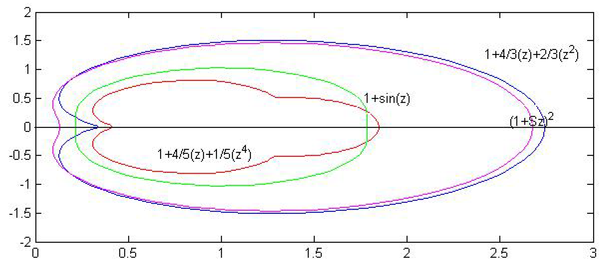
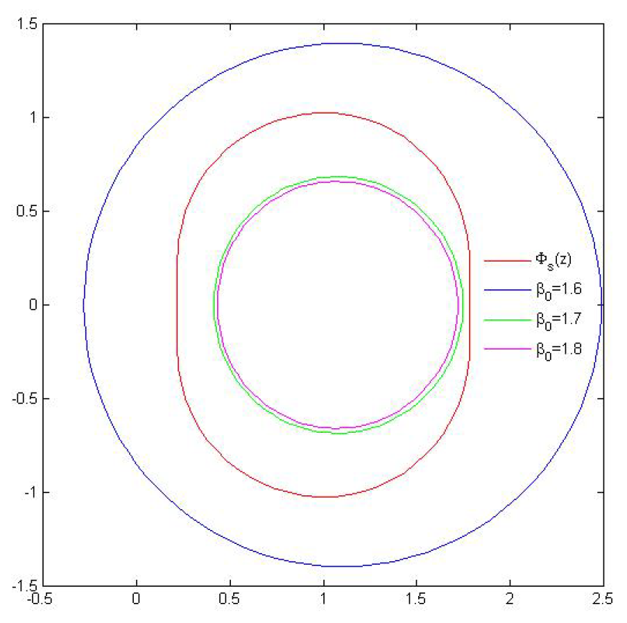
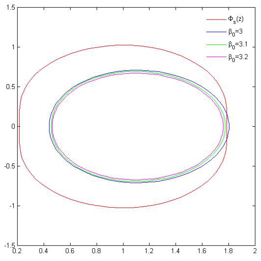
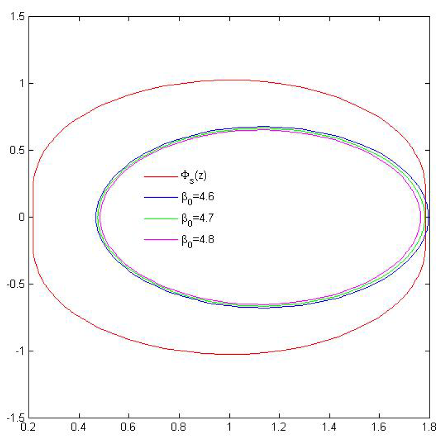
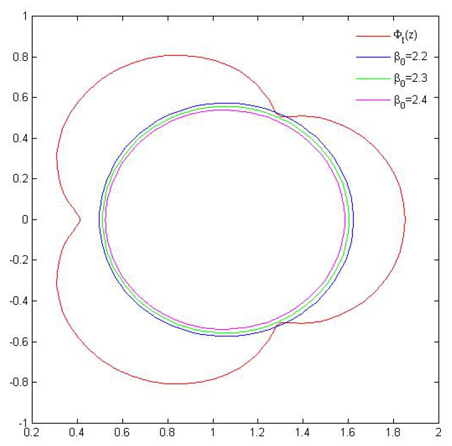
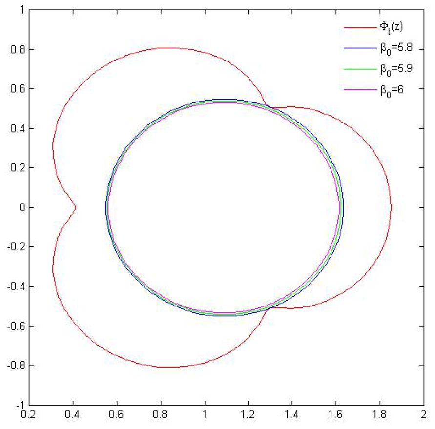
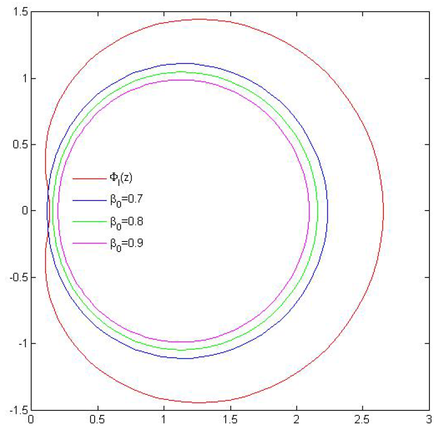
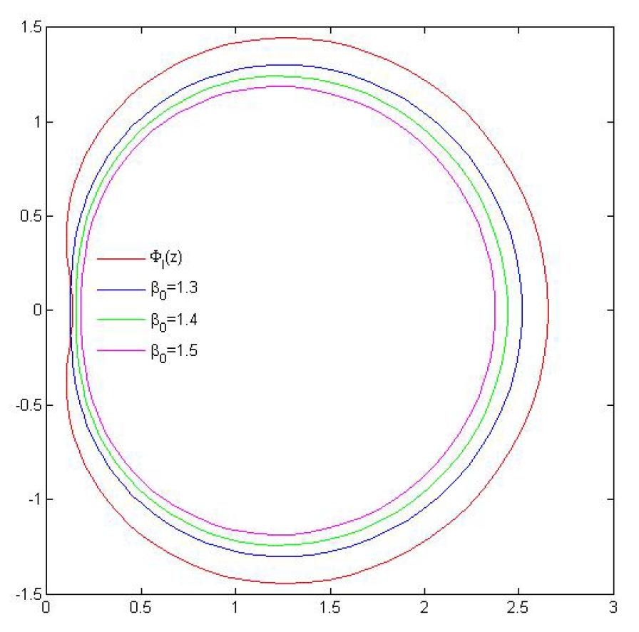
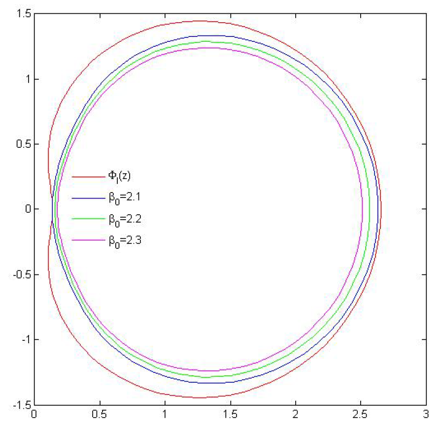
• where we take $S={\displaystyle \frac{7}{10}}$. For $m\in N$, is the value ${\beta }_0={\displaystyle \frac{3}{2}}m-{\displaystyle \frac{3}{4}}$ the best possible value in Theorem 4? We attempt to explore it by experimenting with a graphical depiction of ${\mathbb{F}}_{\beta ,m}(\mathbb{M})$ and ${\varphi }_l(\mathbb{M})$. Here, it is important to note that $\mathbb{F}\subset {\varphi }_l$ when $\mathbb{F}\prec {\varphi }_l$. We thus make our cases for $m=2,3,4$.

For $m=2$, $Re(\beta )>{\displaystyle \frac{240}{119}}$ implies that ${\mathbb{F}}_{\beta ,m}(\mathbb{M})\subset {\varphi }_l(\mathbb{M})$. Moreover, Figure 11 shows that for real $\beta$, the subordination property for which ${\mathbb{F}}_{\beta ,m}(\mathbb{M})\subset {\varphi }_c(\mathbb{M})$ follows for $\beta \ge {\beta }_0$, where ${\beta }_0$ can be any possible value in the interval $(0.7,0.8)$. This result is bounded at ${\beta }_0=0.7$ and also holds for all values of ${\beta }_0>0.8$.

For $m=3$, $Re(\beta )>{\displaystyle \frac{769}{238}}$ implies that ${\mathbb{F}}_{\beta ,m}(\mathbb{M})\subset {\varphi }_l(\mathbb{M})$. Moreover, Figure 12 shows that for real $\beta$, the subordination property for which ${\mathbb{F}}_{\beta ,m}(\mathbb{M})\subset {\varphi }_c(\mathbb{M})$ follows for $\beta \ge {\beta }_0$, where ${\beta }_0$ can be any possible value in the interval $(1.3,1.4)$. This result is bounded at ${\beta }_0=1.3$ and also holds for all values of ${\beta }_0>1.4$.

For $m=4$, $Re(\beta )>{\displaystyle \frac{529}{119}}$ implies that ${\mathbb{F}}_{\beta ,m}(\mathbb{M})\subset {\varphi }_l(\mathbb{M})$. Moreover, Figure 13 shows that for real $\beta$, the subordination property for which ${\mathbb{F}}_{\beta ,m}(\mathbb{M})\subset {\varphi }_c(\mathbb{M})$ follows for $\beta \ge {\beta }_0$, where ${\beta }_0$ can be any possible value in the interval $(2.1,2.2)$. This result is bounded at ${\beta }_0=2.1$ and also holds for all values of ${\beta }_0>2.2$.

4. Conclusions

The main focus of the present research is to investigate the inclusion relation of an ALP with different analytic domains. We derived the admissibility criteria for analytical functions. Moreover, we determined the conditions on the parameters $\beta$ and m, under which ${\mathbb{F}}_{\beta ,m}(\zeta )$ is subordinate to the different analytic domains. The graphical representations provide a clear view of the inclusion relation. The suggested technique accurately reflects subordination tendencies. The investigation of inclusion relations of different analytic domains and associated Laguerre polynomials is a promising area of research that can significantly contribute to various fields of science and mathematics. By exploring these relationships, researchers can develop new mathematical theories, enhance computational methods and create innovative applications across disciplines such as physics, engineering, biology and beyond. This interdisciplinary approach fosters a deeper understanding of fundamental principles and paves the way for future advancements in both theoretical and applied sciences.

References

- Carvajal, M.; Arias, J.M.; Gómez-Camacho, J. Analytic evaluation of Franck-Condon integrals for anharmonic vibrational wave functions. Phys. Rev. A 1999, 59, 3462. [Google Scholar] [CrossRef]
- Chung, Y.S.; Sarkar, T.K.; Jung, B.H.; Salazar-Palma, M.; Ji, Z.; Jang, S.; Kim, K. Solution of time domain electric field integral equation using the Laguerre polynomials. IEEE Trans. Antennas Propag. 2004, 52, 2319–2328. [Google Scholar] [CrossRef]
- Mawhin, J.; Ronveaux, A. Schrödinger and Dirac equations for the hydrogen atom, and Laguerre polynomials. Arch. Hist. Exact Sci. 2010, 64, 429–460. [Google Scholar] [CrossRef]
- Khan, M.K.R. A Study of Laguerre Polynomials and its generalization. Doctoral Dissertation, Aligarh Muslim University, Aligarh, India, 2008. [Google Scholar]
- Ma, W.; Minda, D. A unified treatment of some special classes of univalent functions. In Proceedings of the Conference on Complex Analysis; International Press Inc.: Somerville, MA, USA, 1992; pp. 157–169. [Google Scholar]
- Kanwal, B.; Noor, K.I.; Hussain, S. Properties of Certain Classes of Holomorphic Functions Related to Strongly Janowski Type Function. J. Math. 2021, 2021, 1806174. [Google Scholar] [CrossRef]
- Long, P.; Liu, J.; Gangadharan, M.; Wang, W. Certain subclass of analytic functions based on q-derivative operator associated with the generalized Pascal snail and its applications. AIMS Math. 2022, 7, 13423–13441. [Google Scholar] [CrossRef]
- Srivastava, H.M.; Sabir, P.O.; Eker, S.S.; Wanas, A.K.; Mohammed, P.O.; Chorfi, N.; Baleanu, D. Some m-fold symmetric bi-univalent function classes and their associated Taylor-Maclaurin coefficient bounds. J. Inequalities Appl. 2024, 47, 1–18. [Google Scholar] [CrossRef]
- Gandhi, S. Radius estimates for three leaf function and convex combination of starlike functions. In Mathematical Analysis I: Approximation Theory, Proceedings of the International Conference on Recent Advances in Pure and Applied Mathematics, New Delhi, India, 23–25 October 2018; Springer: Singapore, 2018; pp. 173–184. [Google Scholar]
- Cho, N.E.; Kumar, V.; Kumar, S.S.; Ravichandran, V. Radius problems for starlike functions associated with the sine function. Bull. Iran. Math. Soc. 2019, 45, 213–232. [Google Scholar] [CrossRef]
- Sharma, K.; Jain, N.K.; Ravichandran, V. Starlike functions associated with a cardioid. Afr. Mat. 2016, 27, 923–939. [Google Scholar] [CrossRef]
- Bano, K.; Raza, M. Starlikeness associated with Limacon. Filomat 2023, 37, 851–862. [Google Scholar] [CrossRef]
- Breaz, D.; Panigrahi, T.; El-Deeb, S.M.; Pattnayak, E.; Sivasubramanian, S. Coefficient Bounds for Two Subclasses of Analytic Functions Involving a Limacon-Shaped Domain. Symmetry 2024, 16, 183. [Google Scholar] [CrossRef]
- Saliu, A.; Noor, K.I.; Hussain, S.; Darus, M. Some results for the family of univalent functions related with Limac¸on domain. AIMS Math. 2021, 6, 3410–3431. [Google Scholar] [CrossRef]
- Alahmade, A.; Mujahid, Z.; Tawfiq, F.M.O.; Khan, B.; Khan, N.; Tchier, F. Third Hankel Determinant for Subclasses of Analytic and m-Fold Symmetric Functions Involving Cardioid Domain and Sine Function. Symmetry 2023, 15, 2039. [Google Scholar] [CrossRef]
- Raza, M.; Mushtaq, S.; Malik, S.N.; Sokół, J. Coefficient inequalities for analytic functions associated with cardioid domains. Hacet. J. Math. Stat. 2020, 49, 2017–2027. [Google Scholar] [CrossRef]
- Mondal, S.R. Mapping Properties of Associate Laguerre Polynomials in Leminiscate, Exponential and Nephroid Domain. Symmetry 2022, 14, 2303. [Google Scholar] [CrossRef]
- Miller, S.S.; Mocanu, P.T. Differential Subordinations: Theory and applications, Monographs and Textbooks in Pure and Applied Mathematics 225; CRC Press: Boca Raton, FL, USA, 2000. [Google Scholar]
Disclaimer/Publisher’s Note: The statements, opinions and data contained in all publications are solely those of the individual author(s) and contributor(s) and not of MDPI and/or the editor(s). MDPI and/or the editor(s) disclaim responsibility for any injury to people or property resulting from any ideas, methods, instructions or products referred to in the content. |
© 2024 by the authors. Licensee MDPI, Basel, Switzerland. This article is an open access article distributed under the terms and conditions of the Creative Commons Attribution (CC BY) license (https://creativecommons.org/licenses/by/4.0/).
Share and Cite
Al-Sa’di, S.; Siddiqa, A.; Kanwal, B.; Alamri, M.A.; Hussain, S.; Noor, S. Mapping Properties of Associate Laguerre Polynomial in Symmetric Domains. Symmetry 2024, 16, 1545. https://doi.org/10.3390/sym16111545
Al-Sa’di S, Siddiqa A, Kanwal B, Alamri MA, Hussain S, Noor S. Mapping Properties of Associate Laguerre Polynomial in Symmetric Domains. Symmetry. 2024; 16(11):1545. https://doi.org/10.3390/sym16111545
Chicago/Turabian StyleAl-Sa’di, Sa’ud, Ayesha Siddiqa, Bushra Kanwal, Mohammed Ali Alamri, Saqib Hussain, and Saima Noor. 2024. "Mapping Properties of Associate Laguerre Polynomial in Symmetric Domains" Symmetry 16, no. 11: 1545. https://doi.org/10.3390/sym16111545
APA StyleAl-Sa’di, S., Siddiqa, A., Kanwal, B., Alamri, M. A., Hussain, S., & Noor, S. (2024). Mapping Properties of Associate Laguerre Polynomial in Symmetric Domains. Symmetry, 16(11), 1545. https://doi.org/10.3390/sym16111545