Article

Uncertainly Analysis of Prior Distribution in Accelerated Degradation Testing Bayesian Evaluation Method Based on Deviance Information Criterion

1
Technology and Engineering Center for Space Utilization, Chinese Academy of Sciences, Beijing 100094, China
2
University of Chinese Academy of Sciences, Chinese Academy of Sciences, Beijing 100049, China
*
Author to whom correspondence should be addressed.
Symmetry 2024, 16(2), 160; https://doi.org/10.3390/sym16020160
Submission received: 9 January 2024 / Revised: 25 January 2024 / Accepted: 27 January 2024 / Published: 30 January 2024

Abstract

:
The accelerated degradation testing (ADT) Bayesian evaluation method comprehensively utilizes product degradation data under accelerated stress levels collected over a short period of time and multiple sources of prior information, such as historical information, similar product information, simulation information, etc., to conduct life and reliability evaluation. Through the prior distribution, prior information affects the ADT Bayesian evaluation results ultimately. However, different evaluators may obtain different prior distributions based on the same prior information due to varying experiences or rules, which may lead to differences in the ADT Bayesian evaluation results. Therefore, it is necessary to analyze and study the impact of prior distribution uncertainty on the ADT Bayesian evaluation results while also finding criteria to judge the quality of prior distributions. This paper focuses on the ADT Bayesian evaluation method based on the Wiener process and the Arrhenius relation, studying the influence of different prior distributions on the robustness of ADT Bayesian evaluation results. Additionally, based on the deviance information criterion (DIC), a criterion for selecting prior distributions in the ADT Bayesian evaluation method is proposed. Through carrying out uncertainty analysis of prior distribution in the ADT Bayesian evaluation method, a theoretical system and framework for analyzing prior uncertainty in ADT Bayesian evaluation based on DIC are established, providing a better foundation for the practical application of the ADT Bayesian evaluation method in engineering.

1. Introduction

Through quickly collecting product degradation data in a short period of time, accelerated degradation testing (ADT) technology can fully utilize experimental resources under limited conditions, reduce test duration, and save testing costs. It is very suitable for the evaluation of high-reliability and long-life products [1]. Meanwhile, the Bayesian evaluation method can comprehensively use information from multiple sources and conduct life and reliability assessment through Bayesian information fusion methods, which is suitable for evaluating small-sample products [2]. The ADT Bayesian evaluation method combines ADT technology with Bayesian theory, which can improve its accuracy in reliability assessment of small-sample and long-life products.
In recent years, a great deal of research has been conducted on ADT Bayesian analysis. Prakash, G. [3] conducted reliability analysis work on rolling element bearings and presented two Bayesian hierarchical models—one utilizing the life-time data and the other using the degradation data. Guo, J. [4] proposed three novel Bayesian information fusion models to characterize the inherent relationship between the failure-time data and the degradation data and integrate the heterogeneous data to obtain accurate reliability analysis results with a small sample size. Fan, T.-H. [5] focused on the failure time other than the degradation model and used Bayesian predictive analysis based on the inverse Gaussian process with conjugate priors to deduce the failure time inference, which is associated with the degradation model and its goodness-of-fit test, from a complete Bayesian perspective. However, most of the current research on ADT Bayesian evaluation is focused on modeling, data fusion, posterior inference, and so on. They usually assume a certain prior distribution for analysis, thus overlooking the impact of prior distribution uncertainty on the analysis results [6]. Therefore, the analysis of the impact of different prior distributions on evaluation results and how to choose an appropriate prior distribution is still in need of further research.
In the ADT Bayesian evaluation method, prior distribution is primarily obtained through the product’s own historical test data, similar products’ data, engineering experience, etc. Information accumulated in related work in the field before ADT can all serve as prior information [7]. Rich prior information can bring more convenience to the ADT Bayesian evaluation method, but different evaluators using the same prior information may construct different prior distributions. The difficulty lies in how to transform prior information into an objective understanding of the prior parameters, rather than using subjective information to construct the prior distribution. Ferguson, T.S. [8] pointed out that the construction of prior distributions should have sufficient support for prior information in order to ensure flexibility and generality when using prior distributions for inference. Currently, the construction of prior distributions usually relies on some classical statistical methods, including Jeffreys’ prior [9], reference prior [10], noninformative prior [11], ML-II prior [12], maximum entropy prior [13], maximum data information prior [14], and multi-level prior [15].
Appropriate prior distribution can improve the accuracy of ADT Bayesian evaluation, while unreliable prior distribution may have the opposite effect. Currently, research on prior distribution mainly focuses on how to construct prior distribution. However, there is a lack of criteria for evaluating the accuracy and rationality of the constructed prior distributions [16]. Chipman, H. [17] studied the choice of prior distributions and the impact of this choice on subset selection, computation, and practical analysis. Bayarri, M. [18] presented a new approach called the prior-based Bayes information criterion (PBIC) to prior distribution selection based on Laplace expansions. Villa, C. [19] introduced a novel approach to objectively determining model prior probabilities based on measuring the worth using the Kullback–Leibler divergence between densities from different models. Liu, C.C. [20] showed how Bayes factors can be very sensitive to prior assumptions and discussed model generalizability and the generalization criterion. Currently, there is relatively little research directly focused on the criteria for selecting prior distributions, with most studies drawing on the model selection criteria. Therefore, this paper also considers using the deviance information criterion (DIC) from model selection to conduct research on prior distribution selection.
This article focuses on the research of uncertainty issues for prior distribution. It mainly studies the effect of prior distributions on ADT Bayesian evaluation results and proposes a method for selecting prior distributions based on the DIC. The structure of this paper is as follows: Section 2 provides an introduction to modeling for the ADT Bayesian evaluation method; the Wiener process and the Arrhenius relation are selected as the modeling basis for the degradation model and the accelerated model, respectively. In Section 3, principles of how to construct prior distribution and robustness analysis of prior distribution for the ADT Bayesian method are introduced. Through a brief introduction to the DIC theory, the criterion for selecting prior distributions based on the DIC is considered theoretically feasible. Section 4 introduces a simulation case: different combined forms of distributions representing different types of prior information are selected as the prior input for the ADT Bayesian evaluation method. The robustness of the results of the ADT Bayesian evaluation method under the different distributions is investigated, and the reason for the differences in evaluation results caused by different prior distributions is analyzed. Combining the robustness analysis results, the uncertainty of prior information in the ADT Bayesian evaluation method is quantified based on the DIC. The research on analyzing the uncertainty of prior distributions in ADT Bayesian evaluation based on the DIC provides convenience for the engineering application of ADT Bayesian evaluation methods.

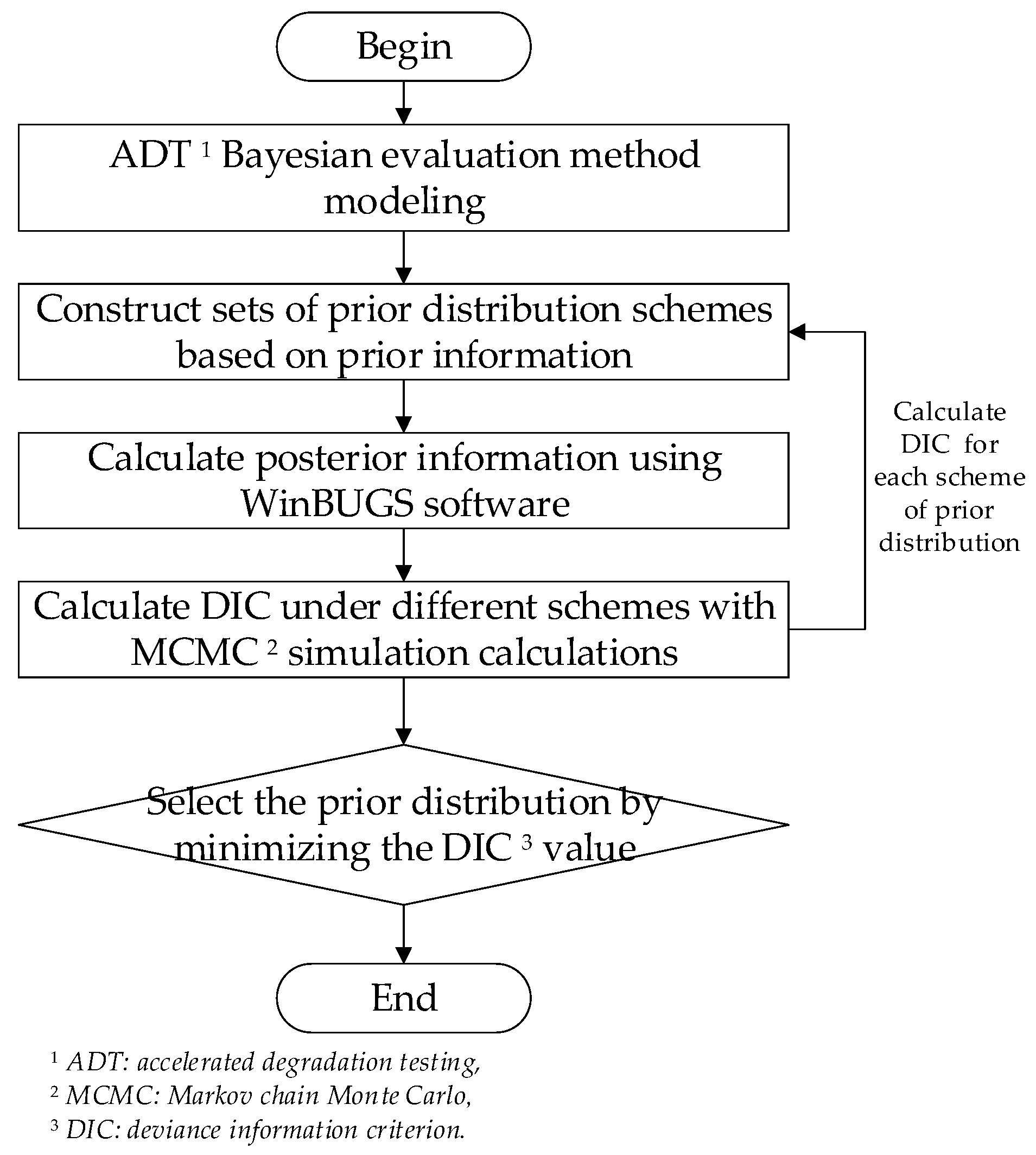
2. Modeling of ADT Bayesian Evaluation

This section introduces the basic process of ADT Bayesian evaluation modeling. The key to ADT Bayesian evaluation modeling lies in two types of models, namely, stochastic process models based on degradation paths and accelerated models describing the relationship between accelerated stress and degradation rate. Currently, scholars have conducted a large amount of relevant research on the modeling of ADT Bayesian. This paper chooses the Wiener process for the degradation model and the Arrhenius relation for the accelerated model, which provides a research foundation for analyzing the impact of prior distributions on ADT Bayesian evaluation.

2.1. Modeling of Accelerated Degradation Processes

When using Bayesian theory to conduct an evaluation of ADT, it is necessary to describe the degradation process of ADT and establish the corresponding ADT model. Stochastic processes can effectively characterize the influence of some stochastic factors in degradation processes and have therefore been widely applied in degradation modeling [21]. The Wiener process, as a stochastic process with continuous time and continuous space parameters, is the most fundamental, simple, and important stochastic process, which has been widely studied in many fields of product degradation modeling [22].
In a traditional ADT scenario, Y(t) is used to represent the degradation process of the product’s performance. Assuming that Y(t) follows a Wiener process with drift constant u and diffusion coefficient σ, the Wiener process can be represented as [23]:
Y t = u t + σ B t .
where B(t) represents the standard Brownian motion. yijk represents the degradation data value at time tijk, where i denotes the number of accelerated stress levels, j denotes the number of samples tested under accelerated stress levels, and k denotes the number of inspections. The degradation increment of the product at time tijk can be represented as:
Δ y t i j k = y i j k y i j k 1 .
Defining the increment of degradation y(t) = Δy(t) as a new form of data. When the degradation process of product performance follows a Wiener process, y(t) follows a normal distribution [2], i.e., y(t)~N (Λ(t), σ2·Λ(t)), where Λ(t) is a non-negative increasing function of time, which is defined as a linear function of time in this paper. The probability density function y(t) is given by
y t ~ 1 σ 2 π Λ t exp y u Λ t 2 2 σ 2 Λ t .
The acceleration model is used to describe the relationship between the acceleration stress s and the degradation rate u [24]. This paper only considers the acceleration model under a single stress. The Arrhenius relation based on failure physics is currently the most widely used acceleration model [25]. Through logarithmic transformation, it can be expressed as a simple linear equation as:
ln u = a + b / s .
where a and b are constant parameters.

2.2. ADT Bayesian Evaluation Model

Bayesian evaluation is a statistical inference based on three types of information (overall information, sample information, and prior information), known as Bayesian statistics [26]. Its main difference from classical probability statistics lies in whether prior information is used for inference analysis. Through the collection, mining, and processing of historical information or empirical knowledge, a prior distribution is formed, which is then incorporated into the statistical analysis of products through data fusion to improve the quality of assessment [27]. The expression for the Bayesian equation is as follows:
π θ | y = f y | θ π θ m y .
where π(θ) is the prior distribution of the prior parameter θ in the absence of sample information. f(y|θ), denoted as a likelihood function, represents the probability distribution of the data y given the parameter θ. The marginal density function m(y) contains no information about the parameter θ; it is a “normalizing” constant that is important for determining the posterior distribution. π(θ|y) is the posterior distribution, which is the description of θ given the sample information of y. The posterior distribution is obtained after integrating the three types of information: overall information, sample information, and prior information.
In the ADT Bayesian evaluation model based on the Wiener process of Equation (3) and the Arrhenius relation of Equation (4), the prior parameters θ include {a, b, σ}. Therefore, the likelihood function of the ADT Bayesian evaluation model is:
l θ | y = f y | θ = i = 1 l j = 1 m i k = 1 n i j f y i j k | a , b , σ .
The logarithmic form of Equation (6) is as follows:
L θ | y = i = 1 l j = 1 m i k = 1 n i j ln σ 1 2 ln 2 π Λ t i j k y i j k exp a + b / s Λ t i j k 2 2 σ 2 Λ t i j k .
By maximizing the logarithmic form of the likelihood function, the maximum likelihood estimation θ ^ = a ^ , b ^ , σ ^ can be obtained. Due to the complexity of the posterior distribution, WinBUGS v.1.4.3 was chosen as calculation software, which can cover the need to estimate the posterior distribution of any parameter of interest in complicated Bayesian models through the Markov chain Monte Carlo (MCMC) method [28]. Doodle in WinBUGS is a graphical interface in which a model can be defined by drawing the corresponding directed acyclic graph (DAG). DAG describes the conditional dependencies of the Bayesian model we wish to fit. Once the model, the data, and the initial values have been specified, the MCMC algorithm can be compiled, run, and iterated to obtain the posterior distribution [29]. Then, through the posterior distribution π(θ|y) = π(a, b, σ|y), the reliability or life expectancy information of the product under normal stress can be evaluated.
The reliability evaluation based on the Wiener process has been studied in reference [30], which suggests that the first-passage time of the Wiener process is a problem-solving of crossing probability distribution for continuous boundary-crossing. Assuming the failure threshold parameter is d, the first-passage time follows an inverse Gaussian distribution, and the reliability function is given by:
R ( t ) = Φ d u Λ ( t ) σ Λ ( t ) exp 2 u d σ 2 Φ d + u Λ ( t ) σ Λ ( t ) .
where Φ(·) is the standard normal cumulative distribution function. In fact, when the value of u is much greater than σ, the latter term of Equation (8) can be ignored, and the Wiener process can be considered non-decreasing [31]. Therefore, the reliability distribution function of first-passage time can be approximated by a normal distribution, i.e., Y(t) is approximately normally distributed with mean Λ(t) and variance σ2·Λ(t).
R t Φ d u Λ t σ Λ t .

3. Uncertainty Analysis of Prior Distributions

This section briefly introduces the principles of how to construct prior distributions, robustness analysis of prior distributions for the ADT Bayesian method, and criteria for prior distribution selection based on DIC. Combined with the ADT Bayes evaluation results and robustness analysis of prior distribution, DIC can prove to be a good selection criterion for prior distribution.

3.1. Principles for Constructing Prior Distributions

According to the theories of the Wiener process for the degradation model and the Arrhenius relation for the accelerated model, θ of the ADT Bayesian evaluation method includes three prior parameters {a, b, σ}. Assuming that the parameters a, b, and σ are independent of each other. To evaluate the impact of different prior distributions on the ADT Bayesian evaluation results, it is possible to consider setting several types of prior distribution schemes with different prior information for each of the three prior parameters. Different forms of prior distributions and different values of parameters can be considered for each type of prior distribution scheme in order to evaluate the uncertainty of different prior distributions.
Based on whether there is prior information that can be referred to, the construction of prior distributions can usually be divided into two categories: one category is when there is prior information available, and the other is when there is no prior information available. In cases with prior information, the construction of a prior distribution can be considered based on prior parameter samples. Cases with the absence of prior information generally refer to situations where there is no historical data or similar product data available for reference in constructing the prior parameters. In this case, non-informative prior distributions are constructed, which typically include Bayesian assumptions, Jeffreys’ prior distribution, reference prior distribution, uniform distribution, etc.
This paper establishes three types of prior distribution schemes in order to conduct an uncertainty analysis of prior distribution. The first type of scheme represents prior distribution combinations of three parameters with biased information, indicating that partial information about the prior parameters, mainly including the mean and variance of the prior parameters, is known through prior information. However, this information is biased with respect to sample information, which is a common occurrence in the Bayesian method during ADT processes. The normal distribution and gamma distribution are often used as representative fitting distributions. The normal distribution is a widely applicable and important probability distribution with characteristics such as centrality, symmetry, and uniform variability, while the gamma distribution is an independent and non-negative probability distribution. Both distributions are well-suited for use as prior parameter distributions. This article selects normal distribution and gamma distribution as specific forms of distribution in these schemes, ensuring that the means and variances of the two types of distributions are the same and examining their impact on the ADT Bayesian evaluation results. The second type of scheme represents prior distribution combinations without prior information, i.e., the mean or variance information of the prior parameters cannot be known through historical information, which is also a common occurrence in the application of ADT Bayesian evaluation. To simplify calculations, it is possible to consider using a uniform distribution over a certain range to replace the non-information prior distribution [32]. The third type of scheme represents prior distribution combinations with accurate prior information, where the mean and variance information of prior distributions is more consistent with sample data information. In such cases, the prior parameters usually have a better fit with the sample data. The purpose of adding the third type of scheme is to analyze the influence of different values of parameters under the same prior distribution on the evaluation results. It can also be understood as a sensitivity analysis of parameters under the same prior distribution.

3.2. Robustness Analysis of Prior Distributions for the ADT Bayesian Method

Uncertainty analysis of prior distributions primarily refers to analyzing the impact of different forms of prior distributions and parameter fluctuations in distributions on the robustness of ADT Bayesian evaluation results. Robustness generally refers to the ability of a product’s performance to remain operational and stable within an acceptable range under the influence of various factors in a specified operating environment or conditions [33]. In uncertainty analysis of prior distributions on the robustness of evaluation results, “specified operating environment” mainly refers to using different prior distributions as input under the same prior information, while “performance” mainly refers to the accuracy of ADT Bayesian evaluation results. Therefore, this paper establishes different prior distribution schemes with different prior information, which contain different types of prior distribution combinations, examining the impact of prior distribution on the ADT Bayesian evaluation results. Robustness analysis of ADT Bayesian evaluation results caused by prior distribution provides input on how to evaluate the quality of prior distribution and how to adjust the modeling of prior distribution. The process of uncertainly analyzing prior distributions based on ADT Bayesian evaluation results is shown in Figure 1.
Step 1: Select an appropriate degradation process and an acceleration model to construct an ADT Bayesian evaluation model for the sample data.
Step 2: For the ADT Bayesian model, build several prior distribution scheme sets {Πv} containing different prior information; each set includes different forms of prior distribution {πi(θ)}.
Step 3: Under the same Bayesian model and sample data, extract πi(θ) from Πv and conduct ADT Bayesian evaluation calculations using WinBUGS software to obtain the posterior distribution {πi(θ|y)}.
Step 4: Based on the posterior distribution, along with the MCMC method [34] and Equation (9), compute the reliability evaluation curve to obtain the ADT Bayesian evaluation results.
Step 5: Return to Step 2, repeat Steps 2~4 for each scheme of prior distribution in set space; obtain evaluation results for all prior distributions.
Step 6: Analyze and compare the posterior distribution of parameters and reliability evaluation results for all different prior distributions, obtaining the impact of prior distribution uncertainty on the robustness of ADT Bayesian evaluation results.

3.3. Criteria for Prior Distribution Selection Based on DIC

DIC was proposed by Spiegelhalter, D.J. [35], which is very suitable for Bayesian model selection problems where the posterior distributions are obtained by MCMC simulation. DIC considers the model’s fit to the data and its own complexity. As the model parameters increase, the fit of the model improves, but the bias function is penalized, leading to an increase in the DIC value. DIC is defined as:
DIC = 2 D θ ¯ D θ ¯ .
where D ( θ ) ¯ represents the mean of deviance for θ, D ( θ ¯ ) represents the deviance of the posterior mean of θ. The expression of deviance of θ is given as follows:
D θ = 2 log f y | θ + C
where C is a constant that cancels out in the calculation of DIC and therefore does not need to be known.
DIC can be calculated through MCMC simulation calculations using WinBUGS software, which is one of the advantages of DIC over other criteria [36]. In fact, DIC was initially proposed mainly for model selection, and a smaller DIC value means better model fitting [35]. However, DIC incorporates both prior information and sample information, ultimately influencing the calculation of DIC values through the posterior distribution. Different posterior distributions resulting from different prior distributions will cause different DIC values to be calculated in the same Bayesian model [37]. Therefore, a smaller DIC value means a better posterior distribution, which is due to the choice of the prior distribution under the same Bayesian model. The prior distribution with a smaller DIC value will be more helpful for posterior evaluation. Combining reliability assessment results under different prior distributions can verify whether the prior distribution selection criteria can effectively evaluate the quality of the prior distributions. The analysis process for selecting prior distributions based on DIC is shown in Figure 2.
Step 1: Build an ADT Bayesian evaluation model.
Step 2: Build sets of prior distribution schemes {Πv}; each set includes different prior distributions {πi(θ)}.
Step 3: Under the same Bayesian model and sample data, extract πi(θ) from Πv, combine with WinBUGS software to conduct an ADT Bayesian evaluation calculation, and obtain the posterior distribution {πi(θ|y)}.
Step 4: Calculate the DIC value based on the posterior distribution, combined with the MCMC method.
Step 5: Go back to Step 2, repeating Steps 2~4 for each scheme in the prior distribution set space; obtain the DIC value for all prior distributions within the set of schemes.
Step 6: Combine the robustness analysis of the uncertainty of prior distribution with the results of the ADT Bayesian evaluation, analyze the characteristics of the DIC values under different sets, and discuss the feasibility of prior distribution selection criteria based on DIC.

4. An Illustrative Simulation Case

4.1. Simulation Data Declaration

In order to study the uncertain analysis of prior distributions, it is necessary to make some certain assumptions for ADT Bayesian evaluation. Through a simulation case, the uncertainty of the prior distribution’s impact on the evaluation results of the ADT Bayesian evaluation method can be analyzed, and the superiority or inferiority of the prior distributions can be judged by DIC. The simulation case is designed for 3 levels of constant stress ADT, whose models consist of the Wiener process for the degradation model and the Arrhenius relation for the accelerated model, which facilitates the analysis and comparison of results. The basic information settings of the illustrative simulation case are shown in Table 1. The reliability curve obtained from the parameters in the table can represent the true reliability level of the product.
The sample data obtained from the simulation based on the parameters in Table 1 are shown in Figure 3. The horizontal axis in the figure represents the measurement time, and the vertical axis represents performance data. If the performance degradation exceeds 30, i.e., the failure threshold d = 30, the product is considered to have failed. This evaluation aims to assess the reliability level of the product under normal operating conditions (T = 45 °C). Based on this simulated data, by comparing the evaluation results under different prior distributions with the evaluation result under the hypothesis parameters of Table 1, the impact of prior distribution uncertainty on the evaluation results can be analyzed, and criteria for selecting prior distributions based on the DIC criterion can be examined.

4.2. Construct Sets of Prior Distributions

To analyze the uncertainty of different prior distributions on the Bayesian evaluation results of ADT, the simulation case builds three different sets Π1, Π2, Π3 for prior distribution schemes.
According to the principles for constructing prior distributions, different combinations of prior distribution forms and parameter settings in Table 2 are set to analyze the influence of different prior distributions on ADT Bayesian results. Π1 represents the prior distribution schemes with biased information. All πi(θ) in Π1 have mean(a)=12, mean(b) = −6000, and mean(σ) = 0.01, which deviates from the hypothesis condition in Table 1. Normal distribution and gamma distribution are selected as prior distribution forms to analyze. In the prior distribution of π1(θ), the parameters a and b are chosen to follow the normal distribution, and σ is chosen to follow the gamma distribution, for it represents the standard deviation in the Wiener process, which has the characteristic of non-negativity. Then, based on π1(θ), different distribution forms are sequentially set for the prior parameters a, b, and σ, totaling 4 combinations, i.e., Π1 = {πi(θ)}, i = 1, 2, 3, 4. Π2 represents the schemes of non-informative prior distributions. Similarly, based on π1(θ) in Π1, prior parameters a, b, and σ are sequentially set to be uniform distribution for non-informative prior, while another combination with all parameters follows uniform distribution, totaling 4 combinations, i.e., Π2={πi(θ)}, i = 5, 6, 7, 8. Π3 represents the prior distribution scheme of precise information. All the prior distributions in Π3 are the same as in Π1, but the parameters’ values of the prior distribution are consistent with the hypothesis condition, which follows mean(a) = 10, mean(b) = −5000, and mean(σ) = 0.005.

4.3. Comparison of Prior and Posterior Distributions

Choosing WinBUGS as calculation software for the posterior parameter estimation of the ADT Bayesian evaluation model. By establishing the Doodle model of the ADT Bayesian method based on the Wiener process and Arrhenius acceleration relation, posterior parameter data can be obtained through Bayesian inference with different prior distributions πi(θ). After conducting 10,000 iterations, the posterior parameter sampling chain stabilizes and converges. Discard the first 5000 data points from the posterior parameter vector as the aging stage, and extract the subsequent 5000 data sample points for the analysis and calculation of the posterior distribution. Figure 4, Figure 5 and Figure 6 show the comparison of prior and posterior distributions for respective parameters under sets of Π1, Π2, and Π3. Combining the changes from the prior distribution with the posterior distribution, partial conclusions regarding the uncertainty analysis of the prior distribution can be drawn.
(1)
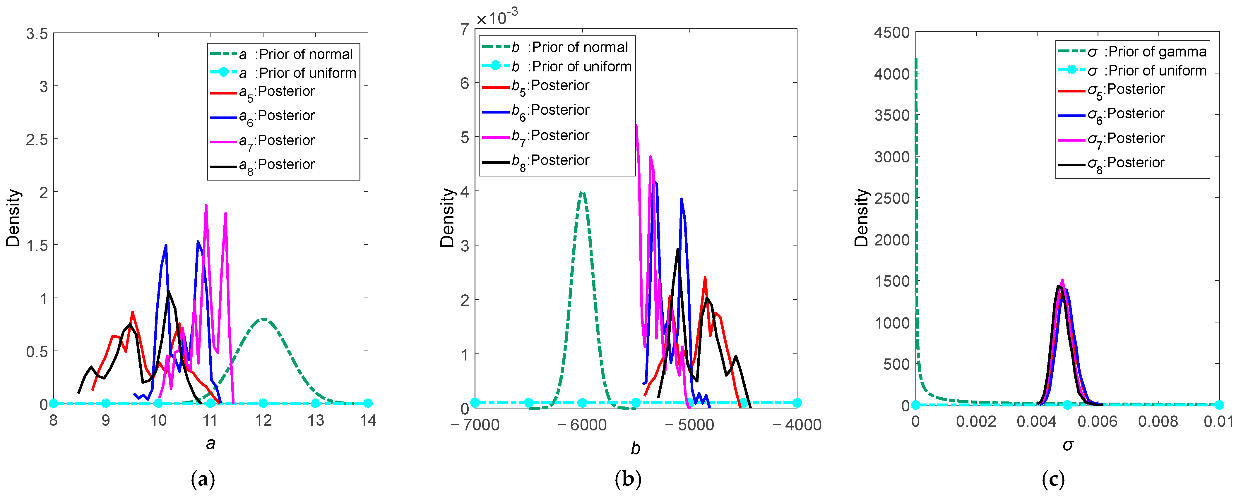
From the comparison graphs, it is obvious that there is a difference between the prior distribution and the posterior distribution. This result is consistent with Bayesian theory, which means that by adjusting the prior distribution based on the sample data, a posterior distribution can be obtained. However, the form of posterior distributions is different from each other, which also indicates that the prior distribution settings do have an impact on ADT Bayesian evaluation results.
(2)
Under Π1, the posterior distributions of a and b are divided into two categories: for πi(θ), i = 1, 2, 4, the posterior distributions of a and b are adjusted by the sample information normally, but posterior distributions do not exhibit obvious distribution characteristics; for π3(θ), when prior parameter b follows a gamma distribution, the prior and posterior distributions of b are almost identical, without the expected adjustment in the posterior distribution, which in turn leads to an unexpected posterior distribution of a.
(3)
Under Π2, both posterior distributions of a and b fluctuate around the original simulated hypothetical values. Compared to Π1, setting non-informative prior distributions has a significant impact on the posterior distributions of a and b. Additionally, whether non-informative prior distributions are chosen between a and b will affect the posterior distribution of the other parameter.
(4)
Under Π3, the posterior distributions of a and b exhibit more noticeable distribution characteristics, with less fluctuation. However, similar to π3(θ), the prior and posterior distributions of parameter b under π11(θ) are almost identical.
(5)
The common feature of π3(θ) and π11(θ) is that the prior parameter b is assigned a gamma distribution. It can be seen from the figure that under the gamma prior distribution, the prior data for parameter b is highly concentrated. But the construction of prior distributions should have sufficient support for prior information. An overconcentrated prior distribution may not be conducive to posterior estimation [8]. Since parameter b represents the coefficient of stress level in the Arrhenius acceleration model, when the prior distribution of b is highly concentrated, it may lead to insufficient adjustment capability of small sample data, thereby affecting the calculation of the posterior distribution for a.
(6)
Under all prior distributions πi(θ), σ exhibits noticeable distribution characteristics with high consistency, indicating that the choice of different prior distributions has little impact on the posterior distribution of σ.
(7)
According to the posterior data points, Table 3 lists the mean, standard deviation (std), 2.5th percentile, and 97.5th percentile of the posterior parameters under different prior distributions in Π1, Π2, and Π3 after convergence of the iterations, for the purpose of comparative analysis. Combining comparison graphs of prior and posterior distributions, it can be concluded as follows:
(1)
Under Π1, for πi(θ|y), i = 1, 2, 4, mean(a) ≈ 10 and mean(b) ≈ −5000, which are close to the values of simulation assumptions. However, for π3(θ|y), mean(a) ≈ 12.7 and mean(b) ≈ −6000, showing a significant deviation from the simulated values.
(2)
In Π2, the posterior means of a and b are close to the simulated values, and std(a) is in the range of 0.3 to 0.6, and std(b) is in the range of 100 to 250, which shows a clear trend of larger standard deviations compared to those of the posterior distribution in Π1. It can be concluded that under non-informative prior distributions, the posterior parameters are not easily converging and exhibit greater fluctuations in this simulation case.
(3)
For the posterior means under Π3, mean(a) ≈ 10 and mean(b) ≈ −5000, with a standard deviation significantly smaller than the posterior parameter standard deviations under Π1 and Π2, making the results more accurate and closer to the simulated hypothesis values.
(4)
Under all prior distributions, the mean of the parameter σ is around 0.005, with a standard deviation of around 0.0003. The 2.5th and 97.5th percentile values are also very close. It can be seen that the different settings of prior distributions have a minor impact on the parameter σ, which is mainly adjusted through the sample data.
(5)
The choice of prior distribution for b has a noticeable impact on the posterior distribution. In π3(θ) and π11(θ), due to the setting of the gamma distribution for b, the posterior distribution’s mean and variance of b are almost identical to the set prior distribution. In the case of π11(θ), although the posterior mean of b is very close to the simulated hypothesis value, its variance still differs significantly from the variances of other posterior distributions under Π3.
(6)
Under Π2, when all three parameters a, b, and σ are assigned non-informative prior distributions, the posterior distribution’s mean achieves results close to the simulated hypothesis condition. This indicates that under non-informative prior distributions, the Bayesian model can effectively find posterior parameters that better match the sample data, but the downside is that the posterior data fluctuates significantly.

4.4. Robustness Analysis of Evaluation Results

Based on 5000 stable and convergent posterior sample data points for each prior distribution, the reliability of the product is calculated. Figure 7 shows the reliability curves of product ADT under the Bayesian evaluation results. The bold red line represents the reliability curve under the hypothesis condition, which can be considered the true performance of the product reliability. The other labeled lines represent the reliability curves for each prior distribution within Π1, Π2, and Π3. From Figure 7, several conclusions can be drawn, as follows:
(1)
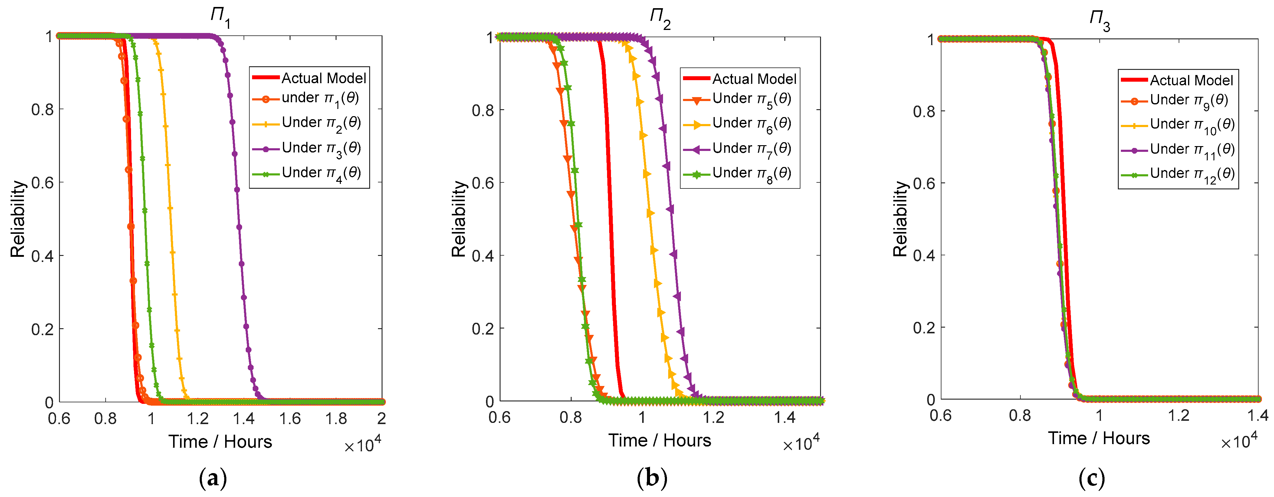
Reliability curves under different prior distributions in Π1 and Π2 have certain differences, even significant disparities, while under different prior distributions in Π3, they are relatively consistent.
(2)
The reliability curve under π1(θ) is quite close to the correct reliability curve. In π1(θ), a and b both use a normal prior distribution, while σ uses a non-negative gamma distribution, which corresponds well to the nature of σ representing the diffusion coefficient of the degradation process. In this setting of prior distribution combination, the reliability curve obtained through the posterior distribution adjusted from the sample data are very accurate. However, the reliability curves under other prior distributions in Π1 deviate from the correct reliability curve.
(3)
In Π2, reliability curves under different prior distributions lie on both sides of the correct reliability curve, showing a certain deviation from each other. Although using non-informative prior distributions, compared to Π1, it still produces results that are close to the correct reliability curve. Therefore, in the absence of explicit prior information, using non-informative prior distributions is not a terribly bad choice for constructing a prior distribution.
(4)
Comparing the reliability curves under π1(θ) with other distributions under Π2, it indicates that when conducting ADT Bayesian evaluation with the correct prior distribution model, prior distributions with biased information will still yield better assessment results than non-informative prior distributions.
(5)
Under Π3, the reliability curves of all prior distributions are highly consistent and very close to the true curve. This is mainly due to the fact that the posterior distribution of a, b, and σ under Π3 is quite consistent and close to the simulated values, with very little fluctuation. This means that when using prior distributions with precise information, the sample data reinforces the prior information, resulting in a smaller variance of the posterior distribution and obtaining a fairly accurate reliability evaluation result.

4.5. Prior Distribution Analysis Based on DIC Value

For prior distributions under Π1, Π2, and Π3, the DIC is used for analysis to compare DIC values under different prior distributions, which are shown in Figure 8. Combining reliability evaluation results under different prior distributions, some conclusions can be drawn as follows:
(1)
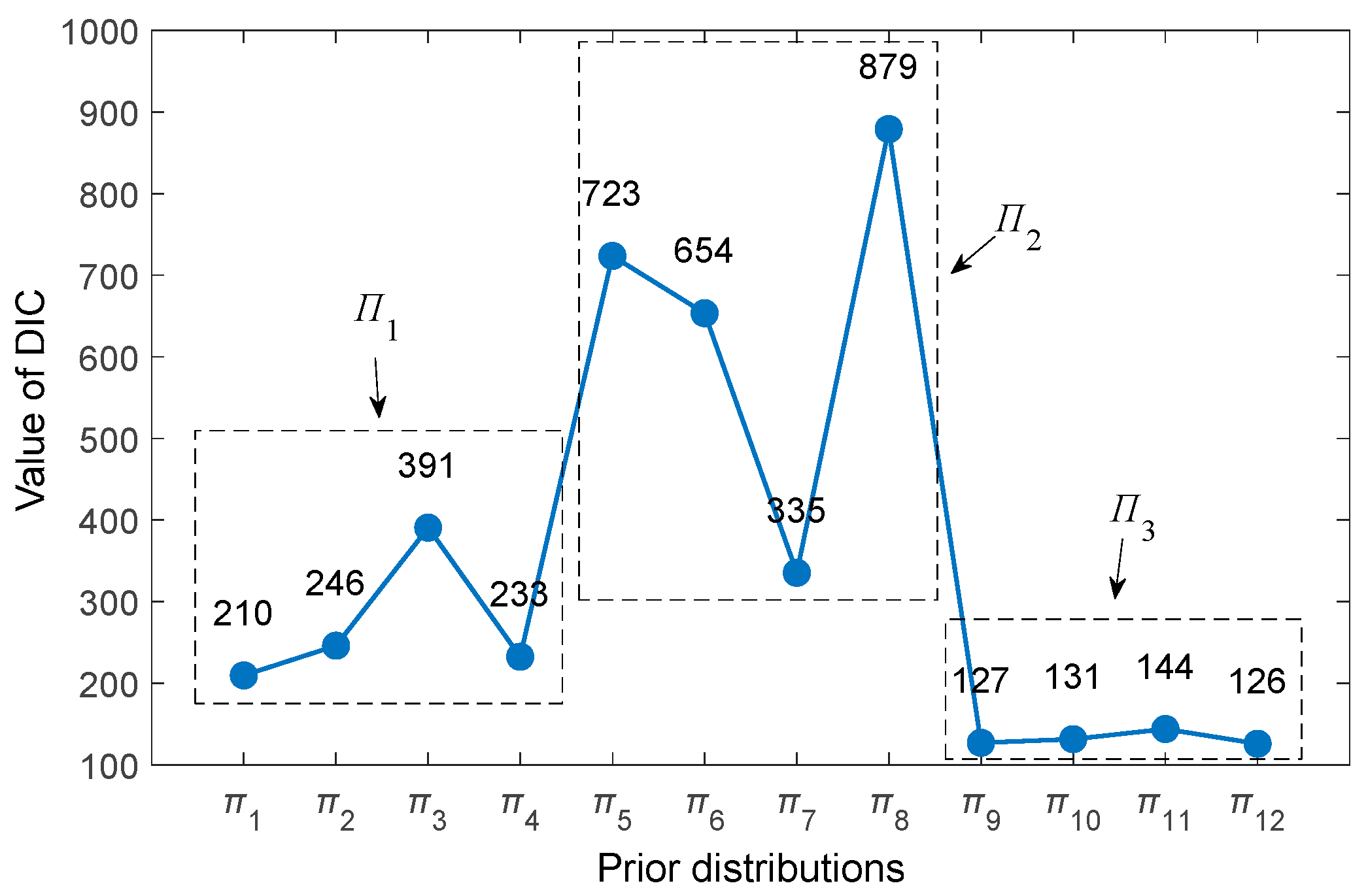
Different prior distribution sets exhibit similarity in DIC values: under Π1, the DIC values are in the range of 200 to 400; under Π2, the DIC values show significant fluctuations, ranging from 300 to 900; under Π3, the DIC values are highly concentrated, ranging from 120 to 150.
(2)
According to the principle of selecting prior distributions based on DIC, which states that a smaller DIC value indicates better model fitting [35]. The performance of DIC values under prior distribution sets allows us to conclude the following ranking: accurate prior information distribution > biased prior information distribution > non-informative prior distribution. Similar conclusions can be found in reference [38]. This indicates that DIC can effectively screen the quality of prior distributions.
(3)
The DIC value of π1(θ) is the smallest in Π1, and the reliability result of π1(θ) is also the best in Π1, correspondingly. Additionally, the issue of significant posterior distribution bias caused by the selection of gamma distribution as the prior distribution for b is also reflected in the DIC values, with the DIC value of π3(θ) being larger than that of other prior distributions.
(4)
The DIC values under Π2 are generally large and exhibit significant fluctuations, indicating that non-informative prior distributions generally yield larger DIC values and are not the optimal choice for prior distributions.
(5)
The relatively smaller DIC values under Π3 indicate that having accurate prior information is significantly beneficial in selecting prior distributions for ADT Bayesian evaluation.
(6)
It is worth noting that the DIC can serve as a guideline for selecting prior distributions, but it is not an absolute rule. This is because in conducting ADT Bayesian evaluation, there may not always be prior information available, or it may not be certain that the prior information obtained matches the true models. Therefore, when using the DIC as a guideline for selecting prior distributions, judgment based on the actual situation is still necessary.

5. Conclusions

This article is based on the ADT Bayesian evaluation method and studies the influence of prior distribution uncertainty on the robustness of the evaluation results. It concludes that the information content and form of the prior distribution both have a certain impact on the ADT Bayesian evaluation method. To address the uncertainty of prior distribution, research on the issue of prior distribution selection for the ADT Bayesian evaluation method is conducted by borrowing from the idea of model selection criteria. DIC is related to the posterior distribution, which is obtained by combining the prior distribution with the sample data. Different posterior distributions resulting from different prior distributions will also cause different DIC values to be calculated in the same Bayesian model. Through the simulation case, it is demonstrated that the DIC can help judge the quality of the prior distribution. Through an uncertain analysis of prior distribution in the ADT Bayesian evaluation method based on DIC, it is possible to fully utilize prior information in engineering practice to develop a more robust and trustworthy ADT Bayesian evaluation method.

Author Contributions

Conceptualization, T.Z. and C.L.; methodology, T.Z.; software, K.L.; validation, W.W.; formal analysis, T.Z.; investigation, K.L.; resources, K.W.; data curation, W.W.; writing—original draft preparation, T.Z.; writing—review and editing, K.L. and W.W.; visualization, K.L.; supervision, C.L.; project administration, K.W.; funding acquisition, T.Z. All authors have read and agreed to the published version of the manuscript.

Funding

This work was supported by the National Natural Science Foundation of China under Grant No. 61703391.

Data Availability Statement

The data presented in this study are available on request from the corresponding author.

Acknowledgments

The authors would like to thank the referees for their careful reading of the manuscript and fruitful comments.

Conflicts of Interest

The authors declare no conflicts of interest.

References

  1. Sun, F.; Liu, L.; Li, X.; Liao, H. Stochastic modeling and analysis of multiple nonlinear accelerated degradation processes through information fusion. Sensors 2016, 16, 1242. [Google Scholar] [CrossRef]
  2. Wang, L.; Pan, R.; Li, X.; Jiang, T. A Bayesian reliability evaluation method with integrated accelerated degradation testing and field information. Reliab. Eng. Syst. Saf. 2013, 112, 38–47. [Google Scholar] [CrossRef]
  3. Prakash, G. A Bayesian approach to degradation modeling and reliability assessment of rolling element bearing. Commun. Stat.-Theory Methods 2021, 50, 5453–5474. [Google Scholar] [CrossRef]
  4. Guo, J.; Li, Y.F.; Peng, W.; Huang, H.Z. Bayesian information fusion method for reliability analysis with failure-time data and degradation data. Qual. Reliab. Eng. Int. 2022, 38, 1944–1956. [Google Scholar] [CrossRef]
  5. Fan, T.-H.; Dong, Y.-S.; Peng, C.-Y. A Complete Bayesian Degradation Analysis Based on Inverse Gaussian Processes. IEEE Trans. Reliab. 2023, 1–13. [Google Scholar] [CrossRef]
  6. Kass, R.E.; Wasserman, L. The selection of prior distributions by formal rules. J. Am. Stat. Assoc. 1996, 91, 1343–1370. [Google Scholar] [CrossRef]
  7. Zou, T.; Dang, W.; Zhang, G.; Liu, K.; Li, P. Prior Distribution Selection Criterion in Accelerated Degradation Testing Bayesian Optimization Design Based on Bayes Factors. In Proceedings of the 2017 International Conference on Sensing, Diagnostics, Prognostics, and Control (SDPC), Shanghai, China, 16–18 August 2017; pp. 694–698. [Google Scholar]
  8. Ferguson, T.S. A Bayesian analysis of some nonparametric problems. Ann. Stat. 1973, 1, 209–230. [Google Scholar] [CrossRef]
  9. Jeffreys, H. The Theory of Probability; OuP Oxford: Oxford, UK, 1998. [Google Scholar]
  10. Sun, D.; Berger, J.O. Reference priors with partial information. Biometrika 1998, 85, 55–71. [Google Scholar] [CrossRef]
  11. Tibshirani, R. Noninformative priors for one parameter of many. Biometrika 1989, 76, 604–608. [Google Scholar] [CrossRef]
  12. Sinha, P.; Bansal, A.K. Bayesian optimization analysis with ML-II ϵ-contaminated prior. J. Appl. Stat. 2008, 35, 203–211. [Google Scholar] [CrossRef]
  13. Handley, W.; Millea, M. Maximum-entropy priors with derived parameters in a specified distribution. Entropy 2019, 21, 272. [Google Scholar] [CrossRef]
  14. Soofi, E.S. Capturing the intangible concept of information. J. Am. Stat. Assoc. 1994, 89, 1243–1254. [Google Scholar] [CrossRef]
  15. Lindley, D.V.; Smith, A.F. Bayes estimates for the linear model. J. R. Stat. Soc. Ser. B Stat. Methodol. 1972, 34, 1–18. [Google Scholar] [CrossRef]
  16. Zou, T.-J.; Li, X.-Y.; Li, M.-J. Impact analysis of prior distributions on ADT Bayesian optimization design based on DIC. In Proceedings of the 2015 Annual Reliability and Maintainability Symposium (RAMS), Palm Harbor, FL, USA, 26–29 January 2015; pp. 1–6. [Google Scholar]
  17. Chipman, H. Prior distributions for Bayesian analysis of screening experiments. In Screening: Methods for Experimentation in Industry, Drug Discovery, and Genetics; Springer: Berlin/Heidelberg, Germany, 2006; pp. 236–267. [Google Scholar]
  18. Bayarri, M.; Berger, J.O.; Jang, W.; Ray, S.; Pericchi, L.R.; Visser, I. Prior-based Bayesian information criterion. Stat. Theory Relat. Fields 2019, 3, 2–13. [Google Scholar] [CrossRef]
  19. Villa, C.; Walker, S. An objective Bayesian criterion to determine model prior probabilities. Scand. J. Stat. 2015, 42, 947–966. [Google Scholar] [CrossRef]
  20. Liu, C.C.; Aitkin, M. Bayes factors: Prior sensitivity and model generalizability. J. Math. Psychol. 2008, 52, 362–375. [Google Scholar] [CrossRef]
  21. Liu, L.; Li, X.; Sun, F.; Wang, N. A general accelerated degradation model based on the Wiener process. Materials 2016, 9, 981. [Google Scholar] [CrossRef] [PubMed]
  22. Tsai, C.-C.; Tseng, S.-T.; Balakrishnan, N. Mis-specification analyses of gamma and Wiener degradation processes. J. Stat. Plan. Inference 2011, 141, 3725–3735. [Google Scholar] [CrossRef]
  23. Park, C.; Padgett, W. Accelerated degradation models for failure based on geometric Brownian motion and gamma processes. Lifetime Data Anal. 2005, 11, 511–527. [Google Scholar] [CrossRef] [PubMed]
  24. Pan, Z.; Balakrishnan*, N. Multiple-steps step-stress accelerated degradation modeling based on Wiener and gamma processes. Commun. Stat.-Simul. Comput. 2010, 39, 1384–1402. [Google Scholar] [CrossRef]
  25. Nelson, W. Analysis of accelerated life test data-part I: The arrhenius model and graphical methods. IEEE Trans. Electr. Insul. 1971, EI-6, 165–181. [Google Scholar] [CrossRef]
  26. Box, G.E.; Tiao, G.C. Bayesian Inference in Statistical Analysis; John Wiley & Sons: Hoboken, NJ, USA, 2011. [Google Scholar]
  27. Li, X.; Hu, Y.; Sun, F.; Kang, R. A Bayesian optimal design for sequential accelerated degradation testing. Entropy 2017, 19, 325. [Google Scholar] [CrossRef]
  28. Ntzoufras, I. Bayesian Modeling Using WinBUGS; John Wiley & Sons: Hoboken, NJ, USA, 2011; Volume 698. [Google Scholar]
  29. Lykou, A.; Ntzoufras, I. WinBUGS: A tutorial. Wiley Interdiscip. Rev. Comput. Stat. 2011, 3, 385–396. [Google Scholar] [CrossRef]
  30. Wang, X.; Wang, B.X.; Wu, W.; Hong, Y. Reliability analysis for accelerated degradation data based on the Wiener process with random effects. Qual. Reliab. Eng. Int. 2020, 36, 1969–1981. [Google Scholar] [CrossRef]
  31. Ye, Z.-S.; Chen, N. The inverse Gaussian process as a degradation model. Technometrics 2014, 56, 302–311. [Google Scholar] [CrossRef]
  32. Nguyen-Trang, T.; Vo-Van, T. A new approach for determining the prior probabilities in the classification problem by Bayesian method. Adv. Data Anal. Classif. 2017, 11, 629–643. [Google Scholar] [CrossRef]
  33. Parkinson, A.; Sorensen, C.; Pourhassan, N. A General Approach for Robust Optimal Design. J. Mech. Des. 1993, 115, 74–80. [Google Scholar] [CrossRef]
  34. Hafez, E.H.; Riad, F.H.; Mubarak, S.A.; Mohamed, M.S. Study on Lindley distribution accelerated life tests: Application and numerical simulation. Symmetry 2020, 12, 2080. [Google Scholar] [CrossRef]
  35. Spiegelhalter, D.J.; Best, N.G.; Carlin, B.P.; Van Der Linde, A. Bayesian measures of model complexity and fit. J. R. Stat. Soc. Ser. B Stat. Methodol. 2002, 64, 583–639. [Google Scholar] [CrossRef]
  36. Ward, E.J. A review and comparison of four commonly used Bayesian and maximum likelihood model selection tools. Ecol. Model. 2008, 211, 1–10. [Google Scholar] [CrossRef]
  37. Berg, A.; Meyer, R.; Yu, J. Deviance information criterion for comparing stochastic volatility models. J. Bus. Econ. Stat. 2004, 22, 107–120. [Google Scholar] [CrossRef]
  38. Grzenda, W. Informative Versus Non-Informative Prior Distributions and their Impact on the Accuracy of Bayesian Inference. Stat. Transition. New Ser. 2016, 17, 763–780. [Google Scholar] [CrossRef]
Figure 1. Robustness analysis of prior distributions on ADT Bayesian evaluation results.
Symmetry 16 00160 g001
Figure 2. Analysis process for selecting prior distributions based on DIC.
Symmetry 16 00160 g002
Figure 3. Degradation paths of simulation data: (a) under 65 °C; (b) under 85 °C; (c) under 100 °C.
Symmetry 16 00160 g003
Figure 4. Comparison graph of prior and posterior distributions in Π1: (a) a; (b) b; (c) σ.
Symmetry 16 00160 g004
Figure 5. Comparison graph of prior and posterior distributions in Π2: (a) a; (b) b; (c) σ.
Symmetry 16 00160 g005
Figure 6. Comparison graph of prior and posterior distributions in Π3: (a) a; (b) b; (c) σ.
Symmetry 16 00160 g006
Figure 7. (a) Reliability curve under Π1; (b) Reliability curve under Π2; (c) Reliability curve under Π3.
Symmetry 16 00160 g007
Figure 8. Comparison graph of DIC values under different prior distributions. DIC: deviance information criterion.
Symmetry 16 00160 g008
Table 1. Basic information settings of the illustrative simulation case.
ContentValues
Degradation processWiener
Accelerated modelArrhenius
Simulation parameter θa = 10, b = −5000, σ = 0.005
Stress levels (Temperature/°C)65, 85, 100
Normal stress level (Temperature/°C)45
Sample size under each stress level6, 6, 6
Monitor times10, 10, 10
Failure threshold30
Table 2. Information settings for sets of prior distributions.
Πkπi(θ)abσ
Π1π1(θ)N(12,1) 1N(−6000,100)Γ(0.1,10)
π2(θ)Γ (144,12)N(−6000,100)Γ(0.1,10)
π3(θ)N(12,1)b~Γ(360,000,60) 2Γ(0.1,10)
π4(θ)N(12,1)N(−6000,100)N(0.01,0.001)
Π2π5(θ)U(−100,100) 3N(6000,100)Γ(0.1,10)
π6(θ)N(12,1)U(−10,000,0)Γ(0.1,10)
π7(θ)N(12,1)N(6000,100)U(0,10)
π8(θ)U(−100,100)U(−10,000,0)U(0,1)
Π3π9(θ)N(10,1)N(−5000,100)Γ(0.05,10)
π10(θ)Γ(100,10)N(−5000,100)Γ(0.05,10)
π11(θ)N(10,1)b~Γ(250,000,50)Γ(0.05,10)
π12(θ) N(10,1)N(−5000,100)N(0.005,0.0005)
1 N(p,q) represents normal distribution. 2 Γ(p,q) represents the gamma distribution. Due to the non-negativity of the gamma distribution, −b~Γ(p,q) represents that the negative of parameter b follows gamma distribution. 3 U(p,q) represents uniform distribution within the interval [p,q].
Table 3. Posterior parameter information for sets of prior distribution schemes.
Πkπi(θ|y)abσ
MeanStd 12.5%97.5%MeanStd2.5%97.5%MeanStd2.5%97.5%
Π1π1(θ|y)10.320.26629.78710.93−511098.04−5336−49130.0050.000290.00450.0056
π2(θ|y)10.690.314110.0911.33−5247115.7−5483−50260.0050.000290.00450.0056
π3(θ|y)12.730.032612.6612.79−59999.981−6018−59790.00530.000310.00470.0059
π4(θ|y)10.220.32729.55710.67−5073120.4−5243−48280.00490.000280.00430.0054
Π2π5(θ|y)9.8330.59138.89910.93−4931217.4−5335−45870.0050.000280.00450.0056
π6(θ|y)10.510.37169.89911.05−5179137−5382−49520.0050.000290.00450.0056
π7(θ|y)10.910.342410.1911.37−5329126−5496−50600.00490.000270.00440.0055
π8(θ|y)9.7490.57568.64910.61−4901211.5−5216−44970.00480.000270.00440.0054
Π3π9(θ|y)10.020.017149.98510.05−50000.5054−5001−49990.0050.000290.00440.0056
π10(θ|y)10.020.017519.98510.05−50000.5019−5001−49990.0050.000290.00440.0056
π11(θ|y)10.020.032029.95410.08−50009.906−5019−49800.0050.00030.00440.0056
π12(θ|y)10.020.016929.98510.05−50000.4979−5001−49990.00480.000270.00440.0054
1 std represents standard deviation.
Disclaimer/Publisher’s Note: The statements, opinions and data contained in all publications are solely those of the individual author(s) and contributor(s) and not of MDPI and/or the editor(s). MDPI and/or the editor(s) disclaim responsibility for any injury to people or property resulting from any ideas, methods, instructions or products referred to in the content.

