A Five-Step Block Method Coupled with Symmetric Compact Finite Difference Scheme for Solving Time-Dependent Partial Differential Equations

Abstract

In this article, we present a five-step block method coupled with an existing fourth-order symmetric compact finite difference scheme for solving time-dependent initial-boundary value partial differential equations (PDEs) numerically. Firstly, a five-step block method has been designed to solve a first-order system of ordinary differential equations that arise in the semi-discretisation of a given initial boundary value PDE. The five-step block method is derived by utilising the theory of interpolation and collocation approaches, resulting in a method with eighth-order accuracy. Further, characteristics of the method have been analysed, and it is found that the block method possesses A-stability properties. The block method is coupled with an existing fourth-order symmetric compact finite difference scheme to solve a given PDE, resulting in an efficient combined numerical scheme. The discretisation of spatial derivatives appearing in the given equation using symmetric compact finite difference scheme results in a tridiagonal system of equations that can be solved by using any computer algebra system to get the approximate values of the spatial derivatives at different grid points. Two well-known test problems, namely the nonlinear Burgers equation and the FitzHugh-Nagumo equation, have been considered to analyse the proposed scheme. Numerical experiments reveal the good performance of the scheme considered in the article.

1. Introduction

Nonlinear partial differential equations are used to model many important physical phenomena that appear in real-world applications of sciences and engineering [1]. It is well-known that the availability of analytical methods for solving nonlinear partial differential equations is limited to a specific class of problems; considering numerical approximations to the solution is one possible way to approach the given problem in this instance [2,3,4,5,6,7]. One ongoing objective in this field is to solve these problems by creating new, efficient numerical schemes or modifying existing ones. Our work in this article examines the approximate solution of time-dependent initial-boundary value PDEs of one dimension in the following form

$$u_t=F(x,t,u,u_x,u_{xx}),\mathrm{with}a\le x\le b,t\ge t_0,$$

(1)

with initial condition

$$u(x,t_0)=\psi \left(x\right),$$

and boundary conditions as

$$u(a,t)={\varphi }_1\left(t\right),u(b,t)={\varphi }_2\left(t\right),$$

where u represents the exact solution of the problem whereas x and t are space and time variables, respectively. In this paper, we actually consider only a special type of Equation (1) in which the second order partial derivative is linear. The spatial semi-discretisation of the above problem (1) converts it into a system of first-order ordinary differential equations in t as follows

$$\frac{dU}{dt}=f(t,U)\mathrm{and}U\left(t_0\right)=U_0,$$

(2)

which can be solved by various existing time integration techniques, for instance, Runge–Kutta or linear multi-step methods [8]. In this article, our focus is on employing a time-marching numerical method of block nature to address the resulting system of first-order ordinary differential equations (ODEs) (2). To assess its performance, we examine two well-known nonlinear time-dependent partial differential equations (PDEs) found in the scientific literature, each with numerous real-world applications. FitzHugh–Nagumo and Burgers’ equations have been analysed numerically using a block approach with a compact finite difference scheme. A nonlinear reaction-diffusion equation, the FitzHugh–Nagumo equation originated in science and technology, particularly in neurophysiology and population growth models, flame propagation, logistic population growth, nuclear reactor theory and catalytic chemical reactions. Some researchers have looked at finite difference and compact difference methods, as in [9,10,11], to obtain numerical solutions of FitzHugh–Nagumo equations.

Another important nonlinear partial differential equation that primarily appears in shock theory and turbulence modelling is the Burgers’ equation. Applications of the Burgers’ equation can be found in many different domains, including quantum fields, traffic flow, fluid dynamics, gas dynamics, shock theory, viscous flow and turbulence. Numerous numerical techniques based on the finite element method, finite difference method, compact finite difference method, MacCormack method, quadrature method, Haar wavelet quasilinearisation approach, splitting methods, etc., have been used in the past to study the Burgers’ equation [12,13,14,15,16,17,18,19,20,21].

Due to their smaller stencil size and increased accuracy, compact finite difference schemes have been more widely used than standard finite difference schemes over the past 50 years [22,23]. Firstly, we develop a five-step block method and combine it with a fourth-order compact finite difference scheme to solve a given problem (1). Block methods are good alternatives for linear multi-step methods that require no starting values to get an approximate solution to a given problem. These methods are self-starting and were first proposed by Milne [24]. With these techniques, multiple points can be approximated simultaneously, saving computation time without sacrificing accuracy [25]. Here, we want to increase the applicability of block methods for solving time-dependent PDEs by combining them with compact finite difference schemes.

2. Development of a Five-Step Block Method

We discretize the time domain $[t_0,t_f]$ with equal step size $k=t_{i+1}-t_i$ for finding the approximate solution of a problem (2). The method for solving a scalar problem $u^{\prime }=f(t,u),u\left(t_0\right)=u_0$ could be applied using a component implementation to solve a system like the one in problem (2). Consider the following polynomial to provide the approximate solution to this problem on an interval $[t_n,t_{n+5}]$ as

$$u\left(t\right)\approx p\left(t\right)=\sum _{n=0}^{n=8}{a}_n{t}^n$$

(3)

where $a_n$ are the constants that must be determined. To differentiate (3) w.r.t.t two times, we get

$$u^{\prime }\left(t\right)\approx p^{\prime }\left(t\right)=\sum _{n=1}^{n=8}n{a}_n{t}^{n-1}$$

(4)

and

$$u^{″}\left(t\right)\approx p^{″}\left(t\right)=\sum _{n=2}^{n=8}n(n-1)a_n{t}^{n-2}$$

(5)

where $a_n$ are the unknown coefficients. To determine the values of nine unknown coefficients, the following interpolatory and collocation conditions are imposed

$$p\left(t_n\right)=u_n,p^{\prime }\left(t_n\right)=f_n,p^{\prime }\left(t_{n+1}\right)=f_{n+1},p^{\prime }\left(t_{n+2}\right)=f_{n+2}$$

$$p^{\prime }\left(t_{n+3}\right)=f_{n+3},p^{\prime }\left(t_{n+4}\right)=f_{n+4},p^{\prime }\left(t_{n+5}\right)=f_{n+5}$$

$$p^{″}\left(t_n\right)=f_n^{\prime },p^{″}\left(t_{n+5}\right)=f_{n+5}^{\prime }$$

Here, $u_{n+j},f_{n+j}$ and $f_{n+j}^{\prime }$ are respectively approximations to $u\left(t_{n+j}\right),u^{\prime }\left(t_{n+j}\right)$ and $u^{″}\left(t_{n+j}\right)$. The above equations can be written in a matrix form as

$$\left[\begin{array}{ccccccccc}1& t_n& t_n^2& t_n^3& t_n^4& t_n^5& t_n^6& t_n^7& t_n^8\\ 0& 1& 2t_n& 3t_n^2& 4t_n^3& 5t_n^4& 6t_n^5& 7t_n^6& 8t_n^7\\ 0& 1& 2t_{n+1}& 3t_{n+1}^2& 4t_{n+1}^3& 5t_{n+1}^4& 6t_{n+1}^5& 7t_{n+1}^6& 8t_{n+1}^7\\ 0& 1& 2t_{n+2}& 3t_{n+2}^2& 4t_{n+2}^3& 5t_{n+2}^4& 6t_{n+2}^5& 7t_{n+2}^6& 8t_{n+2}^7\\ 0& 1& 2t_{n+3}& 3t_{n+3}^2& 4t_{n+3}^3& 5t_{n+3}^4& 6t_{n+3}^5& 7t_{n+3}^6& 8t_{n+3}^7\\ 0& 1& 2t_{n+4}& 3t_{n+4}^2& 4t_{n+4}^3& 5t_{n+4}^4& 6t_{n+4}^5& 7t_{n+4}^6& 8t_{n+4}^7\\ 0& 1& 2t_{n+5}& 3t_{n+5}^2& 4t_{n+5}^3& 5t_{n+5}^4& 6t_{n+5}^5& 7t_{n+5}^6& 8t_{n+5}^7\\ 0& 0& 2& 6t_n& 12t_n^2& 20t_n^3& 30t_n^4& 42t_n^5& 56t_n^6\\ 0& 0& 2& 6t_{n+5}& 12t_{n+5}^2& 20t_{n+5}^3& 30t_{n+5}^4& 42t_{n+5}^5& 56t_{n+5}^6\end{array}\right]\left[\begin{array}{c}{a}_0\\ a_1\\ a_2\\ a_3\\ a_4\\ a_5\\ a_6\\ a_7\\ a_8\end{array}\right]=\left[\begin{array}{c}{u}_n\\ f_n\\ f_{n+1}\\ f_{n+2}\\ f_{n+3}\\ f_{n+4}\\ f_{n+5}\\ f_n^{\prime }\\ f_{n+5}^{\prime }\end{array}\right]$$

Using the Mathematica system, the values of the nine unknowns that appear in the above system of equations have been determined. By substituting these values and changing the variable t to $t_n+mk$, the polynomial in (3) can be re-written as

$$p(t_n+mk)=b_0{u}_n+k(b_1{f}_n+b_2{f}_{n+1}+b_3{f}_{n+2}+b_4{f}_{n+3}+b_5{f}_{n+4}+b_6{f}_{n+5})+k^2(b_7{f}_n^{\prime }+b_8{f}_{n+5}^{\prime })$$

(6)

where the coefficients $b_j^{\prime }s$ are continuous functions of variable m. After evaluating the above polynomial for $m=1,2,3,4,5$, we get a complete structure of the block method that consists of the following five formulas

$$\begin{array}{cc}\hfill u_{n+1}& =u_n+\frac{k}{\mathrm{6,048,000}}(\mathrm{3,068,391}{f}_n+\mathrm{3,678,525}{f}_{n+1}-\mathrm{1,128,100}{f}_{n+2}+\mathrm{663,900}{f}_{n+3}\hfill \\ \hfill & -\mathrm{353,475}{f}_{n+4}+\mathrm{118,759}{f}_{n+5})+\frac{60k^2}{\mathrm{6,048,000}}(7899f_n^{\prime }-731f_{n+5}^{\prime })\hfill \\ \hfill u_{n+2}& =u_n+\frac{k}{\mathrm{189,000}}(\mathrm{844,431}{f}_n+\mathrm{214,650}{f}_{n+1}+\mathrm{85,900}{f}_{n+2}-8600f_{n+3}\hfill \\ \hfill & +2025f_{n+4}-418f_{n+5})+\frac{k^2}{\mathrm{189,000}}(\mathrm{11,220}{f}_n^{\prime }+120f_{n+5}^{\prime })\hfill \\ \hfill u_{n+3}& =u_n+\frac{k}{\mathrm{224,000}}(\mathrm{106,213}{f}_n+\mathrm{231,975}{f}_{n+1}+\mathrm{230,100}{f}_{n+2}+\mathrm{118,100}{f}_{n+3}\hfill \\ \hfill & -\mathrm{20,025}{f}_{n+4}+5637f_{n+5})+\frac{k^2}{\mathrm{224,000}}(\mathrm{15,420}{f}_n^{\prime }-1980f_{n+5}^{\prime })\hfill \\ \hfill u_{n+4}& =u_n+\frac{k}{\mathrm{23,625}}(\mathrm{10,686}{f}_n+\mathrm{26,100}{f}_{n+1}+\mathrm{20,600}{f}_{n+2}+\mathrm{27,600}{f}_{n+3}\hfill \\ \hfill & +\mathrm{10,350}{f}_{n+4}-836f_{n+5})+\frac{240k^2}{\mathrm{23,625}}(6f_n^{\prime }+f_{n+5}^{\prime })\hfill \\ \hfill u_{n+5}& =u_n+\frac{k}{\mathrm{48,384}}(\mathrm{22,835}{f}_n+\mathrm{50,625}{f}_{n+1}+\mathrm{47,500}{f}_{n+2}+\mathrm{47,500}{f}_{n+3}\hfill \\ \hfill & +\mathrm{50,625}{f}_{n+4}+\mathrm{22,835}{f}_{n+5})+\frac{3300k^2}{\mathrm{48,384}}(f_n^{\prime }-f_{n+5}^{\prime })\hfill \end{array}$$

(7)

The above method is a five-step second derivative block method that will simultaneously yield approximations of solutions to the initial-value problems (2) at the nodal points $t_{n+1},t_{n+2},t_{n+3},t_{n+4}$ and $t_{n+5}$.

3. Basic Characteristics of the Method and Stability Analysis

This section discusses various characteristics of the block method (7).

3.1. Order of Accuracy and Consistency

Consider a difference operator ${\mathcal{L}}_j$ related to the five-step block method given by (7)

$$\mathcal{L}\left[u\right(t),k]=u(t+jk)-$$

$$F_j[k,u\left(t\right),u^{\prime }\left(t\right),u^{\prime }(t+k),u^{\prime }(t+2k),u^{\prime }(t+3k),u^{\prime }(t+4k),u^{\prime }(t+5k),u^{\prime \prime }\left(t\right),u^{\prime \prime }(t+5k)]$$

(8)

with $j=1,2,3,4,5$ and $F_j$ is the corresponding right-hand side of each formula. Expanding the expression (8) using Taylor’s series about the point t and combining the like terms in k, the local truncation errors of each formula given in (7) are obtained as

$${\mathcal{LTE}}_1=\frac{-3061u^9\left(t\right)k^9}{6350400}+O\left(k^{10}\right)$$

$${\mathcal{LTE}}_2=\frac{-113u^9\left(t\right)k^9}{1587600}+O\left(k^{10}\right)$$

$${\mathcal{LTE}}_3=\frac{-33u^9\left(t\right)k^9}{78400}+O\left(k^{10}\right)$$

$${\mathcal{LTE}}_4=\frac{-u^9\left(t\right)k^9}{9925}+O\left(k^{10}\right)$$

$${\mathcal{LTE}}_5=\frac{-125u^9\left(t\right)k^9}{254016}+O\left(k^{10}\right)$$

The above expressions for local truncation errors conclude that the proposed method has eighth-order accuracy, implying that the proposed block method is consistent.

3.2. Zero Stability

The block method (7) is said to be zero-stable if the roots of its first characteristic equation $\rho \left(\lambda \right)=0$ have modulus < 1, and the roots of modulus one must be simple. By considering the limit as k tends to zero, from the method (7), we get

$$I{U}_n-R{U}_{n-1}=0$$

where $U_n={(U_{n+1},U_{n+2},U_{n+3},U_{n+4},U_{n+5})}^T$ and $U_{n-1}={(U_{n-4},U_{n-3},U_{n-2},U_{n-1},U_n)}^T$

$$R=\left[\begin{array}{ccccc}0& 0& 0& 0& 1\\ 0& 0& 0& 0& 1\\ 0& 0& 0& 0& 1\\ 0& 0& 0& 0& 1\\ 0& 0& 0& 0& 1\end{array}\right]$$

and I is the identity matrix of order five. The characteristic equation for the above method is $\rho \left(\lambda \right)=det(R-\lambda I)={\lambda }^4(1-\lambda )=0$. The roots are $\{0,0,0,0,1\}$. It implies that the five-step block method is zero-stable.

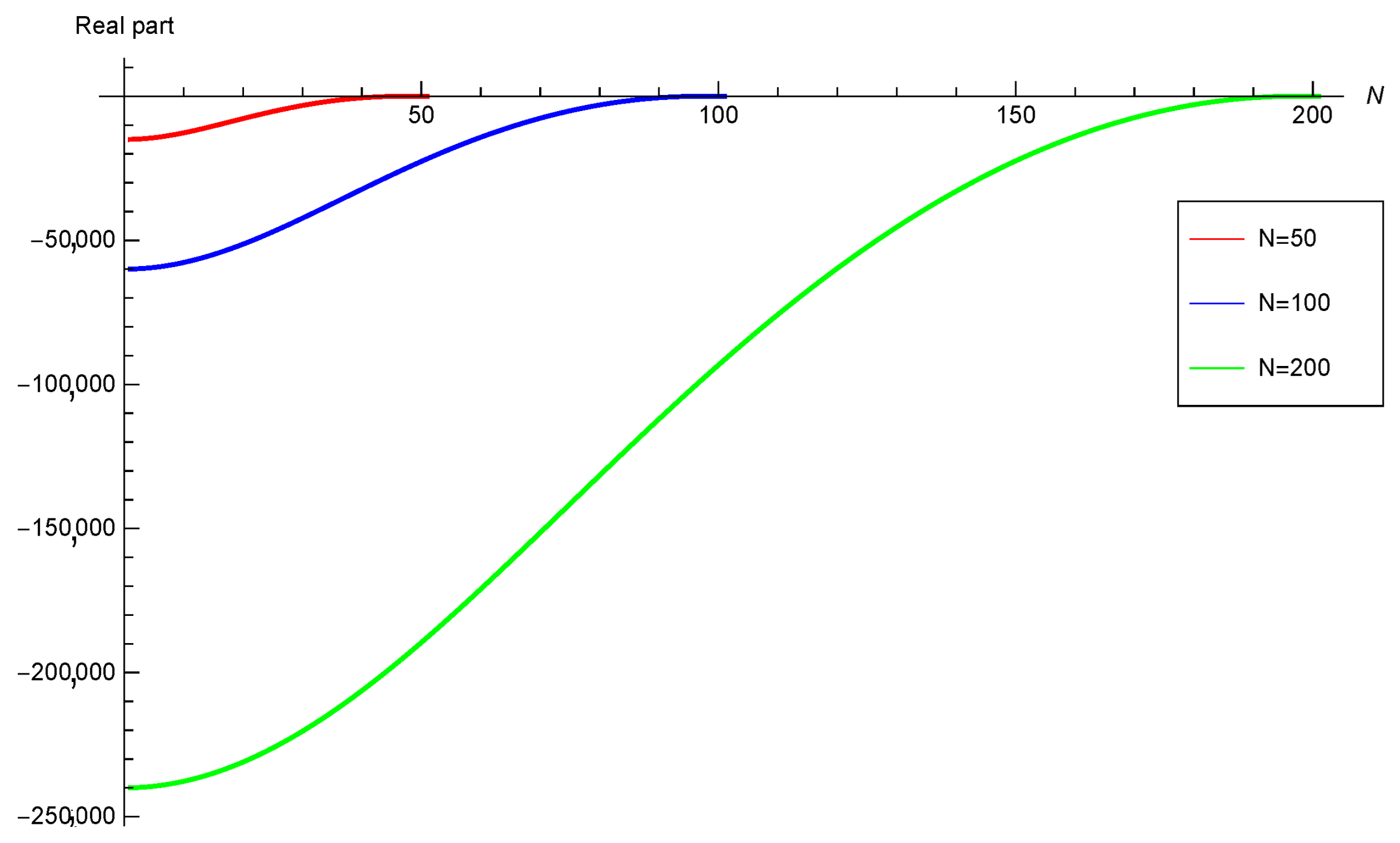
3.3. Linear Stability Analysis

The linear stability analysis of a numerical scheme is carried out by applying it to Dahlquist’s test equation

$$u^{\prime }=\lambda u,Re\left(\lambda \right)<0.$$

(9)

As t approaches ∞, any true solution $c{e}^{\lambda t}$ to the above Equation (9) will decay. For the numerical method to be stable, the behaviour of the numerical solution should match the nature of the true solution. After substituting $\lambda k=\overline{k}$ and appying the proposed block method to Equation (9), we obtain a difference system in matrix form as

$$L\left[\begin{array}{c}{u}_{n+1}\\ u_{n+2}\\ u_{n+3}\\ u_{n+4}\\ u_{n+5}\end{array}\right]=M\left[\begin{array}{c}{u}_{n-4}\\ u_{n-3}\\ u_{n-2}\\ u_{n-1}\\ u_n\end{array}\right]$$

where matrices L and M are respectively given as

$$L=\left[\begin{array}{ccccc}1-\frac{3678525\overline{k}}{6048000}& \frac{1128100\overline{k}}{6048000}& \frac{-663900\overline{k}}{6048000}& \frac{353475\overline{k}}{6048000}& \frac{418\overline{k}+43860{\overline{k}}^2}{6048000}\\ \frac{-214650\overline{k}}{189000}& 1-\frac{85900\overline{k}}{189000}& \frac{8600\overline{k}}{189000}& \frac{-2025\overline{k}}{189000}& \frac{418\overline{k}-120{\overline{k}}^2}{189000}\\ \frac{-231975\overline{k}}{224000}& \frac{-230100\overline{k}}{224000}& 1-\frac{118100\overline{k}}{224000}& \frac{20025\overline{k}}{224000}& \frac{-5637\overline{k}+1980{\overline{k}}^2}{224000}\\ \frac{-26100\overline{k}}{23625}& \frac{-20600\overline{k}}{23625}& \frac{-27600\overline{k}}{23625}& 1-\frac{10350\overline{k}}{23625}& \frac{836\overline{k}-240{\overline{k}}^2}{23625}\\ \frac{-50625\overline{k}}{48384}& \frac{-47500\overline{k}}{48384}& \frac{-47500\overline{k}}{48384}& \frac{-50625\overline{k}}{48384}& 1+\frac{-22835\overline{k}+3300{\overline{k}}^2}{48384}\end{array}\right]$$

$$M=\left[\begin{array}{ccccc}0& 0& 0& 0& 1+\frac{3068391\overline{k}+3068391{\overline{k}}^2}{6048000}\\ 0& 0& 0& 0& 1+\frac{84443\overline{k}+11220{\overline{k}}^2}{189000}\\ 0& 0& 0& 0& 1+\frac{106213\overline{k}+15420{\overline{k}}^2}{224000}\\ 0& 0& 0& 0& 1+\frac{10686\overline{k}+240{\overline{k}}^2}{23625}\\ 0& 0& 0& 0& 1+\frac{22835\overline{k}+3300{\overline{k}}^2}{48384}\end{array}\right]$$

Thus, we have

$$\left[\begin{array}{c}{u}_{n+1}\\ u_{n+2}\\ u_{n+3}\\ u_{n+4}\\ u_{n+5}\end{array}\right]=N\left(\overline{k}\right)\left[\begin{array}{c}{u}_{n-4}\\ u_{n-3}\\ u_{n-2}\\ u_{n-1}\\ u_n\end{array}\right]$$

where the matrix $N\left(\overline{k}\right)=L^{-1}M$ is the stability matrix. To find out the stability characteristics of the block method, we consider the spectral of the stability matrix $\{0,0,0,0,P\left(\overline{k}\right)\}$ where

$$P\left(\overline{k}\right)=\frac{3360+8400\overline{k}+9600{\overline{k}}^2+6500{\overline{k}}^3+2798{\overline{k}}^4+745{\overline{k}}^5+100{\overline{k}}^6}{3360-8400\overline{k}+9600{\overline{k}}^2-6500{\overline{k}}^3+2798{\overline{k}}^4-745{\overline{k}}^5+100{\overline{k}}^6}$$

The region of absolute stability [26] is given by

$$S=\{\overline{k}\in C:|P\left(\overline{k}\right)|<1\}$$

The given method (7) is said to be A-stable if the left half of the complex plane is contained within S. In Figure 1, the absolute stability region of method (7) has been plotted, indicating its A-stability.

4. Symmetric Compact Finite Difference Scheme

To discretise the spatial derivatives appearing in a given PDE (1), we have used symmetric compact finite difference schemes rather than conventional finite difference approximations to spatial derivatives—the reason for considering this because due to their better accuracy and smaller stencils compared to the traditional finite difference scheme. Note that discretisation of spatial derivatives present in the given PDE using symmetric compact finite difference schemes results in a tridiagonal system of equations that can be easily handled by Mathematica software. Many researchers have developed compact schemes with various boundary conditions and different orders, as in [27,28].

Discretise the space variable $a<x<b$ into N subintervals of equal length $h=x_{i+1}-x_i$ where $i=1,2,3\dots \dots ,N+1$.

Consider a fourth-order compact finite difference scheme for discretising the first-order spatial derivative appearing in (1) at the interior nodes $i=2,3,4\dots \dots ,N.$

$$\frac{1}{4}{u}_{i-1}^{\prime }+u_i^{\prime }+\frac{1}{4}{u}_{i+1}^{\prime }=\frac{3}{4h}(u_{i+1}-u_{i-1})$$

where the prime denotes the derivative concerning the space variable and the following one-sided boundary scheme to obtain approximations at boundary points given

for $i=1$

$$u_1^{\prime }+3u_2^{\prime }=\frac{1}{h}\left(-\frac{17}{6}{u}_1+\frac{3}{2}{u}_2+\frac{3}{2}{u}_3-\frac{1}{6}{u}_4\right)$$

and for $i=N+1$

$$u_{N+1}^{\prime }+3u_N^{\prime }=\frac{1}{h}\left(\frac{17}{6}{u}_{N+1}-\frac{3}{2}{u}_N-\frac{3}{2}{u}_{N-1}+\frac{1}{6}{u}_{N-2}\right).$$

The above equations can be written in a matrix form given by

$$A_1{U}^{\prime }=B_{1}U$$

(10)

$$A_1={\left[\begin{array}{ccccccc}1& 3& 0& 0& \cdots & 0& 0\\ 1/4& 1& 1/4& 0& \cdots & 0& 0\\ 0& 1/4& 1& 1/4& \cdots & 0& 0\\ ⋮& \ddots & \ddots & \ddots & \ddots & 0& 0\\ 0& 0& 0& 0& \cdots & 1/4& 0\\ 0& 0& 0& 0& \cdots & 1& 1/4\\ 0& 0& 0& 0& \cdots & 3& 1\end{array}\right]}_{(N+1)\times (N+1)}$$

$$B_1=\frac{1}{2h}{\left[\begin{array}{cccccccc}17/3& 3& 3& -1/3& 0& \cdots & 0& 0\\ -3/2& 0& 3/2& 0& 0& \cdots & 0& 0\\ 0& -3/2& 0& 3/2& 0& \cdots & 0& 0\\ ⋮& \ddots & \ddots & \ddots & \ddots & \ddots & 0& 0\\ 0& 0& 0& \cdots & -3/2& 0& 3/2& 0\\ 0& 0& 0& \cdots & 0& -3/2& 0& 3/2\\ 0& 0& 0& \cdots & 1/3& -3& -3& -17/3\end{array}\right]}_{(N+1)\times (N+1)}$$

$$U={\left[\begin{array}{c}{U}_1\\ U_2\\ U_3\\ .\\ .\\ .\\ U_N\\ U_{N+1}\end{array}\right]}_{(N+1)\times 1}$$

Solving the above system of equations, we can obtain approximations to first-order space derivatives at the discrete points of interest.

Similarly, to approximate the second spatial derivative appearing in the equation, we consider the following fourth-order compact finite difference scheme for interior nodes $i=2,3,\dots N$ given by

$$\frac{1}{10}{u}_{i-1}^{″}+u_i^{″}+\frac{1}{10}{u}_{i+1}^{″}=\frac{6}{5h^2}\left(u_{i+1}-2u_i+u_{i-1}\right).$$

For boundary points, we have:

for $i=1,$

$$u_1^{″}+10u_2^{″}=\frac{1}{h^2}\left(\frac{145}{12}{u}_1-\frac{76}{3}{u}_2+\frac{29}{2}{u}_3-\frac{4}{3}{u}_4+\frac{1}{12}{u}_5\right)$$

and for $i=N+1$

$$u_{N+1}^{″}+10u_N^{″}=\frac{1}{h^2}\left(\frac{145}{12}{u}_{N+1}-\frac{76}{3}{u}_N+\frac{29}{2}{u}_{N-1}-\frac{4}{3}{u}_{N-2}+\frac{1}{12}{u}_{N-3}\right)$$

The complete matrix system for the tridiagonal fourth-order compact scheme for approximating the second derivative can be written as follows

$$A_2{U}^{″}=B_{2}U$$

(11)

$$A_2={\left[\begin{array}{ccccccc}1& 10& 0& 0& \cdots & 0& 0\\ 1/10& 1& 1/10& 0& \cdots & 0& 0\\ 0& 1/10& 1& 1/10& \cdots & 0& 0\\ ⋮& \ddots & \ddots & \ddots & \ddots & 0& 0\\ 0& 0& 0& 0& \cdots & 1/10& 0\\ 0& 0& 0& 0& \cdots & 1& 1/10\\ 0& 0& 0& 0& \cdots & 10& 1\end{array}\right]}_{(N+1)\times (N+1)}$$

$$B_2=\frac{1}{h^2}{\left[\begin{array}{ccccccccc}145/12& -76/3& 29/2& -4/3& 1/12& 0& \cdots & 0& 0\\ 6/5& -12/5& 6/5& 0& 0& 0& \cdots & 0& 0\\ 0& 6/5& -12/5& 6/5& 0& 0& \cdots & 0& 0\\ ⋮& \ddots & \ddots & \ddots & \ddots & \ddots & \ddots & 0& 0\\ 0& 0& 0& 0& \cdots & 6/5& -12/5& 6/5& 0\\ 0& 0& 0& 0& 0& \cdots & 6/5& -12/5& 6/5\\ 0& 0& 0& \cdots & 1/12& -4/3& 29/2& -76/3& 145/12\end{array}\right]}_{(N+1)\times (N+1)}$$

$$U={\left[\begin{array}{c}{U}_1\\ U_2\\ U_3\\ .\\ .\\ .\\ U_N\\ U_{N+1}\end{array}\right]}_{(N+1)\times 1}$$

Solving the above system of equations, one can get an approximation to the second-order space derivatives appearing in the equation at the discrete points of interest.

5. Test Problems

The two well-known nonlinear problems, Burgers’ and FitzHugh–Nagumo equations, will be solved using the above combined numerical scheme based on the block method in conjunction with a compact finite difference scheme. Additionally, special consideration has been given to the stability of the resulting differential systems.

5.1. Burgers’ Equation

Consider the one-dimensional Burgers’ equation:

$$u_t+u{u}_x=v{u}_{xx}$$

(12a)

with the initial condition

$$u(x,0)=\psi \left(x\right);a\le x\le b,$$

(12b)

and two boundary conditions are given as

$$u(a,t)={\varphi }_1\left(t\right)=u_1\left(t\right)andu(b,t)={\varphi }_2\left(t\right)=u_{N+1}\left(t\right),t\ge 0.$$

(12c)

where u represents fluid’s velocity, v is the kinematic viscosity and $xandt$ are the space and time variables, respectively. The system of first-order ODEs derived from (12a)–(12c) can be expressed as follows after semi-discretisation:

$$\left[\begin{array}{c}{u}_1^{\prime }\\ u_2^{\prime }\\ \cdots \\ u_N^{\prime }\\ u_{N+1}^{\prime }\end{array}\right]=v\left(A_2^{-1}{B}_2\right)\left[\begin{array}{c}{u}_1\\ u_2\\ \cdots \\ u_N\\ u_{N+1}\end{array}\right]-\left[\begin{array}{c}{u}_1\\ u_2\\ \cdots \\ u_N\\ u_{N+1}\end{array}\right]\circ \left(A_1^{-1}{B}_1\right)\left[\begin{array}{c}{u}_1\\ u_2\\ \cdots \\ u_N\\ u_{N+1}\end{array}\right]$$

where “∘” indicates the elementwise product of two matrices of the same dimensions. The above system can be expressed in a compact form as

$$U^{\prime }=CU+D$$

(13)

where $C=v\left(A_2^{-1}{B}_2\right)$ is an $(N+1)times(N+1)$ matrix and the D matrix contains non-linear terms.

5.2. FitzHugh–Nagumo Equation

Consider the FitzHugh–Nagumo equation:

$$u_t=u_{xx}+u(1-u)(u-\mathsf{\mu })$$

(14a)

with initial condition

$$u(x,0)=\psi \left(x\right);a\le x\le b,$$

(14b)

and boundary conditions

$$u(a,t)={\varphi }_1\left(t\right)=u_1\left(t\right)andu(b,t)={\varphi }_2\left(t\right)=u_{N+1}\left(t\right),t\ge 0.$$

(14c)

where x and t are space and time variables, respectively. The spatial derivatives in this equation will be approximated using a fourth-order compact finite difference scheme. After semi-discretisation, the system of first-order ODEs obtained from (14a)–(14c) can be expressed as follows

$$\left[\begin{array}{c}{u}_1^{\prime }\\ u_2^{\prime }\\ \cdots \\ u_N^{\prime }\\ u_{N+1}^{\prime }\end{array}\right]=(A_2^{-1}{B}_2-\mathsf{\mu }I)\left[\begin{array}{c}{u}_1\\ u_2\\ \cdots \\ u_N\\ u_{N+1}\end{array}\right]+(1+\mathsf{\mu })\left[\begin{array}{c}{u}_1^2\\ u_2^2\\ \cdots \\ u_N^2\\ u_{N+1}^2\end{array}\right]-\left[\begin{array}{c}{u}_1^3\\ u_2^3\\ \cdots \\ u_N^3\\ u_{N+1}^3\end{array}\right]$$

The above system can be written as

$$U^{\prime }=CU+D$$

(15)

where $C=(A_2^{-1}{B}_2-\mathsf{\mu }I)$ is an $(N+1)\times (N+1)$ matrix and the D matrix contains non-linear terms.

5.3. Stability of Differential System

To examine the stability of the differential systems for the considered PDEs, semidiscretise the problem by applying a compact finite difference scheme to the spatial derivatives in the Equation (1). This will result in a system of ODEs of the form

$$U^{\prime }=CU+D$$

(16)

where C is an $(N+1)$ square matrix and D is an $(N+1)\times 1$ vector containing nonhomogeneous parts.

The matrix for the Burgers’ equation can be written as

$$C=v{C}_2$$

and the matrix for the FitzHugh–Nagumo equation is

$$C=(C_2-\mathsf{\mu }I)$$

For both of the PDEs, the matrix $C_2$ is given by $C_2=A_2^{-1}{B}_2$.

To find out the stability of differential system (16), we linearise the non-linear terms appearing in both PDEs by assuming the value of $u(x,t)=U_j$ is constant. Thus, the stability of the ensuing linear differential system will imply the stability of the non-linear differential system. The stability of the differential system is related to the eigenvalues of matrix C. It is said to be stable if the real part of each eigenvalue is either zero or negative. This has been validated for the two differential systems under investigation for the various spatial grid points depicted in Figure 2 and Figure 3. The differential system is stable in both cases.

6. Numerical Experiments

In this section, some numerical experiments have been presented to illustrate the performance of the block method in conjunction with a compact finite difference scheme. We have used Wolfram Mathematicaversion 11.0 for performing numerical computations. The standard formulas are utilized to compute the $L_{\infty }$ and $L_{rms}$ errors [29,30]

$$L_{\infty }=\underset{1\le i\le N+1}{max}\left|e_i\right|$$

$$L_{rms}={\left(\sum _{i=1}^{N+1}\frac{e_i^2}{N+1}\right)}^{1/2}$$

where

$$e_i=u(x_i,t)-U(x_i,t).$$

Here, $u(x_i,t)$ and $U(x_i,t)$ represent the analytical and numerical solutions at the point $(x_i,t)$, respectively.

6.1. Nonlinear Burgers’ Equation

6.1.1. Example 1

We consider the initial and boundary conditions for the Burgers’ equation in (12a) given by

$$u(x,0)=sin\left(\pi x\right),0\le x\le 1$$

$$u(0,t)=u(1,t)=0,t>0$$

The exact solution is given as [16]

$$u(x,t)=2v\pi \frac{{\sum }_{n=1}^{\infty }{a}_{n}exp(-n^2{\pi }^{2}vt)nsinn\pi x}{a_0+{\sum }_{n=1}^{\infty }exp(-n^2{\pi }^{2}vt)cosn\pi x}$$

with the Fourier coefficients

$$a_0={\int }_0^{1}exp{(-2v\pi )}^{-1}[1-cos\left(\pi x\right)]dx$$

$$a_n=2{\int }_0^{1}exp{(-2v\pi )}^{-1}[1-cos\left(\pi x\right)]cosn\pi xdx,n=1,2,3...$$

In Figure 4, we have plotted the exact solution of the given PDE and its numerical solution obtained by the proposed method for a specific value of time $t=0.5$ by considering various grid points as $x=0.1,0.3,0.5,0.7,0.9$ with $N=100, k=0.001$ and $v=0.01$. It shows that the physical behavior of both solutions is similar.

6.1.2. Example 2

Consider the test problem (12a) taking $v=0.01$ and $a=2$ subject to the initial and boundary conditions given by

$$u(x,0)=\frac{2v\pi sin\left(\pi x\right)}{a+cos\left(\pi x\right)},0\le x\le 1$$

$$u(0,t)=u(1,t)=0,t>0$$

gives the exact solution to the problem [20]

$$u(x,t)=\frac{2v\pi sin\left(\pi x\right){exp}^{-{\pi }^{2}vt}}{a+cos\left(\pi x\right){exp}^{-{\pi }^{2}vt}}$$

Table 1. Absolute error at $t=0.1$.

x	Absolute Error
0.1	4.6342 × ${10}^{-9}$
0.2	1.4033 × ${10}^{-10}$
0.3	1.9936 × ${10}^{-9}$
0.4	1.2330 × ${10}^{-10}$
0.5	4.9473 × ${10}^{-9}$
0.6	2.3491 × ${10}^{-8}$
0.7	3.8157 × ${10}^{-8}$
0.8	6.0069 × ${10}^{-8}$
0.9	1.5378 × ${10}^{-8}$

presents absolute errors for $t=0.1$ by applying the proposed scheme for $N=20,k=0.001$. It demonstrates that the proposed scheme integrates the given problem accurately.

In

Table 2. Comparison of results with $v=1$ and $N=40$.

x	Absolute Error (Asai [31])	Absolute Error (Mittal [20])	Absolute Error (The Proposed Scheme)
0.1	4.50 × ${10}^{-5}$	7.40 × ${10}^{-5}$	3.84 × ${10}^{-8}$
0.2	7.70 × ${10}^{-5}$	6.00 × ${10}^{-6}$	5.45 × ${10}^{-9}$
0.3	1.21 × ${10}^{-4}$	1.20 × ${10}^{-5}$	6.79 × ${10}^{-9}$
0.4	2.40 × ${10}^{-5}$	1.78 × ${10}^{-4}$	1.23 × ${10}^{-9}$
0.5	2.53 × ${10}^{-4}$	3.90 × ${10}^{-5}$	4.41 × ${10}^{-8}$
0.6	3.56 × ${10}^{-4}$	4.40 × ${10}^{-5}$	1.63 × ${10}^{-7}$
0.7	4.84 × ${10}^{-4}$	1.00 × ${10}^{-5}$	2.53 × ${10}^{-7}$
0.8	3.32 × ${10}^{-4}$	7.40 × ${10}^{-5}$	3.48 × ${10}^{-7}$
0.9	4.17 × ${10}^{-4}$	2.81 × ${10}^{-4}$	7.86 × ${10}^{-7}$

and

Table 3. Comparison of results with $v=0.5$ and $N=40$.

x	Absolute Error (Asai [31])	Absolute Error (Mittal [20])	Absolute Error (The Proposed Scheme)
0.1	4.00 × ${10}^{-6}$	0.000000	5.76 × ${10}^{-10}$
0.2	9.00 × ${10}^{-6}$	2.00 × ${10}^{-6}$	1.47 × ${10}^{-9}$
0.3	1.40 × ${10}^{-5}$	3.00 × ${10}^{-6}$	1.96 × ${10}^{-9}$
0.4	2.20 × ${10}^{-5}$	6.00 × ${10}^{-6}$	2.82 × ${10}^{-10}$
0.5	3.20 × ${10}^{-5}$	1.00 × ${10}^{-5}$	9.95 × ${10}^{-9}$
0.6	4.90 × ${10}^{-5}$	1.20 × ${10}^{-5}$	4.02 × ${10}^{-9}$
0.7	7.50 × ${10}^{-5}$	7.50 × ${10}^{-5}$	6.72 × ${10}^{-9}$
0.8	4.50 × ${10}^{-5}$	1.00 × ${10}^{-4}$	1.58 × ${10}^{-9}$
0.9	8.10 × ${10}^{-5}$	7.40 × ${10}^{-5}$	3.35 × ${10}^{-7}$

, absolute error of the proposed scheme has been compared with [20] and [31] for various values of v and $t=0.001$. We use the same number of time steps as in [20]. It shows that the proposed scheme offers better results.

Table 4. ${\mathcal{L}}_{\infty }$-error and ROC.

N	${\mathcal{L}}_{\mathit{\infty }}$-Error	ROC
40	8.08777 × ${10}^{-9}$
80	9.97993 × ${10}^{-10}$	3.0186
160	3.83759 × ${10}^{-11}$	4.7008
320	1.69230 × ${10}^{-12}$	4.5031

shows the Rate of Convergence (ROC) of the proposed scheme in the spatial direction for the values $v=0.01$, $t=0.001$ and $k=0.0001$. It can be observed from Table 4 that the ROC agrees with the theoretical order of convergence of the proposed scheme in the spatial direction.

6.2. Non-Linear FitzHugh–Nagumo Equation

6.2.1. Example 1

Consider the test problem (14a) using $\mathsf{\mu }=0.75$ along with initial condition as

$$u(x,0)=\frac{1}{2}+\frac{1}{2}tanh\left(\frac{x}{2\sqrt{2}}\right),-10\le x\le 10.$$

The exact solution to the problem is [9]

$$u(x,t)=\frac{1}{2}+\frac{1}{2}tanh\left(\frac{x}{2\sqrt{2}}-\frac{(2\mathsf{\mu }-1)t}{4}\right)$$

Table 5. Comparison of $L_{\infty }$-error norm at time $t=0.2$.

N	${\mathit{L}}_{\mathit{\infty }}$-Error with CPU (sec.) (The Proposed Scheme)	${\mathit{L}}_{\mathit{\infty }}$ (Method in Akkoyunlu [9])
12	6.3673 × ${10}^{-4}$	3.9857 × ${10}^{-4}$
	(0.65)
24	4.7712 × ${10}^{-5}$	2.3475 × ${10}^{-5}$
	(2.34)
48	8.0504 × ${10}^{-6}$	8.3749 × ${10}^{-6}$
	(9.60)
64	4.7818 × ${10}^{-6}$	5.9363 × ${10}^{-6}$
	(17.75)
No. of iterations	4	20

compares the $L_{\infty }$ error norm using the proposed scheme with some available data from Akkoyunlu [9] for different values of N at time $t=0.2$. With the proposed scheme, we have almost the same or even better accuracy in the numerical approximation after just four applications, while the scheme presented in Akkoyunlu [9] has reached similar accuracy after 20 time steps. As a result, the proposed scheme produced similar errors in fewer iterations, saving computational effort.

In

Table 6. Comparison with different approaches for Example1 with $\mathsf{\mu }=0.75$ and $N=100$.

	Ahmad [32]	Jiwari [11]	The Proposed Scheme
$\mathit{t}$	${\mathcal{L}}_{\mathbf{rms}}$-Errorh	${\mathcal{L}}_{\mathbf{rms}}$-Error	${\mathcal{L}}_{\mathbf{rms}}$-Error with CPU (sec.)
0.2	2.1960 × ${10}^{-7}$	1.5880 × ${10}^{-5}$	4.0099 × ${10}^{-7}$
			(47.89)
0.5	1.5696 × ${10}^{-6}$	3.8433 × ${10}^{-5}$	2.8629 × ${10}^{-6}$
			(125.23)
1.0	7.1449 × ${10}^{-6}$	8.1870 × ${10}^{-5}$	1.3175 × ${10}^{-5}$
			(268.56)
1.5	1.7262 × ${10}^{-5}$	1.3387 × ${10}^{-4}$	3.2282 × ${10}^{-5}$
			(395.18)
2	3.1857 × ${10}^{-5}$	1.9433 × ${10}^{-4}$	6.1114 × ${10}^{-5}$
			(527.95)
time step-size(k)	0.0001	0.001	0.01

, we have compared the $L_{rms}$ error for this problem using the proposed scheme with the results from Ahmad et al. [32] and Jiwari et al. [11] for $N=100$ and $v=0.75$ at different values of time. It must be mentioned here that the proposed scheme integrates the given problem with a large time step size and produces similar accuracy in just four iterations. In contrast, the approaches presented in [11,32] achieve similar accuracy with smaller time steps resulting in many iterations. Thus, the proposed method provides better or equal results for fewer iterations.

6.2.2. Example 2

Consider the test problem given by (14a) taking $\mathsf{\mu }=0.5$ along with the initial condition as

$$u(x,0)=\frac{1}{1+exp(\frac{-x}{\sqrt{2}})},0\le x\le 1.$$

where the exact solution is given by [33].

Table 7. Comparison of maximum absolute error for Example 2 with $\mathsf{\mu }=0.5$ and $t=0.04$.

x	The Proposed Scheme	ExpFDM [33]	ANM [33]
0.2	2.5011 × ${10}^{-7}$	3.00 × ${10}^{-6}$	2.00 × ${10}^{-7}$
0.4	3.5686 $\times {10}^{-7}$	1.00 $\times {10}^{-5}$	5.00 × ${10}^{-7}$
0.6	1.0422 × ${10}^{-7}$	2.00 × ${10}^{-5}$	7.00 × ${10}^{-7}$
0.8	9.7036 × ${10}^{-7}$	4.00 × ${10}^{-5}$	6.00 × ${10}^{-7}$
No. of iterations	1	8	8

compares errors produced by the proposed scheme and the approaches given in [33]. The errors produced by the schemes in Inan et al. [33] called ANM and ExpFDM are bigger than those obtained using the proposed scheme. Also, note that the proposed scheme uses only one iteration to integrate the problem.

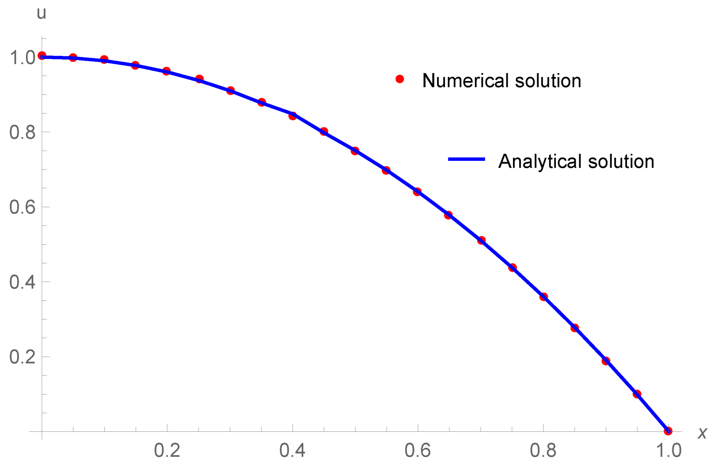
6.3. PDE with Manufactured Solution

Consider the PDE

$$u_t-u_{xx}-u^2=f(x,t)$$

(17)

whose exact solution will be manufactured. We will formulate its solution with the help of a technique called Method of manufactured solutions (MMS). In this method, we choose a function $u(x,t)$, which satisfies the initial and two boundary conditions. For the above PDE, one choice is $u(x,t)=xsint+1-x^2$. So, we substitute this value into the above differential equation to find $f(x,t)$.

Thus, we have the exact solution $u(x,t)=xsint+1-x^2$ to the initial-boundary value problem:

$$u_t-u_{xx}-u^2=xcost+2+x^2{sin}^{2}t+{(1-x^2)}^2+2x(1-x^2)sint0\le t\le T,0<x<1$$

(18)

with initial condition

$$u(x,0)=1-x^2$$

and boundary conditions

$$u(0,t)=1,u(1,t)=sint.$$

In Figure 5, we have plotted the manufactured solution of the given PDE and its numerical solution obtained by the proposed method, demonstrating the proposed method’s good performance.

7. Conclusions

This article considers a five-step block method coupled with a compact finite difference scheme for numerically integrating time-dependent initial-boundary value PDEs. Theoretical development of the block method and its basic characteristics have been presented. The block method has very good stability characteristics with eighth-order accuracy. Further, a combined numerical scheme is obtained by coupling the block method with a compact finite difference scheme. The effectiveness of the presented approach has been demonstrated by applying it to two well-known test problems: Burgers’ equation and FitzHugh–Nagumo equation. The approach considered in this article is a good alternative for solving the types of problems considered in the article.

References

1. Debnath, L. Nonlinear Partial Differential Equations for Scientists and Engineers; Birkhauser: Basel, Switzerland, 2012. [Google Scholar]
2. Collatz, L. The Numerical Treatment of Differential Equations, 1st ed.; Springer: Berlin/Heidelberg, Germany, 1966. [Google Scholar]
3. Li, H.-B.; Song, M.-Y.; Zhong, E.-J.; Gu, X.-M. Numerical Gradient Schemes for Heat Equations Based on the Collocation Polynomial and Hermite Interpolation. Mathematics 2019, 7, 93. [Google Scholar] [CrossRef]
4. Luo, W.-H.; Huang, T.-Z.; Gu, X.-M.; Liu, Y. Barycentric rational collocation methods for a class of nonlinear parabolic partial differential equations. Appl. Math. Lett. 2017, 68, 13–19. [Google Scholar] [CrossRef]
5. Mehta, A.; Singh, G. Solving one-dimensional third order nonlinear KdV equation using MacCormack method coupled with compact finite difference scheme. AIP Conf. Proc. 2022, 2451, 020064. [Google Scholar]
6. Parvizi, M.; Khodadadian, A.; Eslahchi, M.R. A mixed finite element method for solving coupled wave equation of Kirchhoff type with nonlinear boundary damping and memory term. Math. Method Appl. Sci. 2021, 44, 12500–12521. [Google Scholar] [CrossRef]
7. Parvizi, M.; Khodadadian, A.; Eslahchi, M.R. Analysis of Ciarlet-Raviart mixed finite element methods for solving Boussinesq equation. J. Comput. Appl. Math. 2020, 379, 112818. [Google Scholar] [CrossRef]
8. Butcher, J.C. Numerical Methods for Ordinary Differential Equations, 2nd ed.; John Wiley & Sons: Hoboken, NJ, USA, 2008. [Google Scholar]
9. Akkoyunlu, C. Compact finite difference method for Fitz-Hugh-Nagumo equation. Univ. J. Math. Appl. 2019, 4, 180–187. [Google Scholar] [CrossRef]
10. Agbavon, K.M.; Appadu, A.R. Construction and analysis of some nonstandard finite difference methods for the Fitz-Hugh-Nagumo equation. Numer. Differ. Equ. 2020, 36, 1145–1169. [Google Scholar] [CrossRef]
11. Jiwari, R.; Gupta, R.; Kumar, V. Polynomial differential quadrature method for numerical solutions of the generalized Fitzhugh-Nagumo equation with time-dependent coefficients. Ain Shams Eng. 2014, 5, 1343–1350. [Google Scholar] [CrossRef]
12. Jiwari, R. A haar wavelet quasilinearization approach for numerical simulation of Burgers’ equation. Comput. Phys. Commun. 2012, 183, 2413–2423. [Google Scholar] [CrossRef]
13. Jiwari, R. A hybrid numerical scheme for the numerical solution of Burgers’ equation. Comput. Phys. Commun. 2015, 188, 59–67. [Google Scholar] [CrossRef]
14. Benton, E.; Platzman, G.W. A table of solutions of the one-dimensional Burgers’ equations. Quart. Appl. Math. 1972, 30, 195–212. [Google Scholar] [CrossRef]
15. Zhang, P.G.; Wang, J.P. A predictor-corrector compact finite difference scheme for Burgers’ equation. Appl. Math. Comput 2012, 219, 892–898. [Google Scholar] [CrossRef]
16. Sari, M.; Gurarslan, G. A sixth-order compact finite difference scheme to numerical solution of Burgers’ equation. Appl. Math. Comput. 2009, 208, 475–483. [Google Scholar] [CrossRef]
17. Gao, F.; Chi, C. Numerical solution of non-linear Burgers’ equation using high accuracy multi-quadric quasi interpolation. Appl. Math. Comput. 2014, 229, 414–421. [Google Scholar] [CrossRef]
18. Hassanian, I.A.; Salama, A.A.; Hosham, H.A. Fourth-order finite difference method for solving Burgers’ equation. Appl. Math. Comput. 2005, 170, 892–898. [Google Scholar] [CrossRef]
19. Yang, X.; Ge, Y.; Zhang, L. A class of high-order compact difference schemes for solving the Burgers’ equation. Appl. Math. Comput. 2019, 358, 394–417. [Google Scholar] [CrossRef]
20. Mittal, R.C.; Jain, R.K. Numerical solution of non-linear Burgers’ equation with modified cubic b-splines collocation method. Appl. Math. Comput. 2012, 358, 7839–7855. [Google Scholar] [CrossRef]
21. Gulsu, M. A finite difference approach for solution of Burgers’ equation. Appl. Math. Comput. 2006, 175, 1245–1255. [Google Scholar] [CrossRef]
22. Lele, S.K. Compact finite difference schemes with spectral-like resolution. J. Comput. Phys. 1992, 103, 16–42. [Google Scholar] [CrossRef]
23. Zhao, J. Highly accurate compact mixed methods for two point boundary value problems. Appl. Math. Comput. 2017, 188, 1402–1418. [Google Scholar] [CrossRef]
24. Milne, W.E. Numerical Solution of Differential Equations; Wiley: New York, NY, USA, 1953; Volume 9. [Google Scholar]
25. Lambert, J.D. Computational methods in ordinary differential equations. In Introductory Mathematics for Scientists and Engineers; Wiley: New York, NY, USA, 1973; Volume 54. [Google Scholar]
26. Harrier, E.; Wanner, G. Solving Ordinary Differential Equations-II: Stiff and Differential-Algebraic Problems; Springer: Berlin/Heidelberg, Germany, 1996. [Google Scholar]
27. Tyler, G.J. Analysis and Implementation of High-Order Compact Finite Difference Schemes. Master’s Thesis, Brigham Young University, Provo, UT, USA, 2007. [Google Scholar]
28. Mehra, M.; Patel, K.S. A suite of Compact Finite Difference Schemes. ACM Trans. Math. Softw. 2017, 44, 1–31. [Google Scholar] [CrossRef]
29. Erdogan, L.; Sakar, M.G.; Saldir, O. A finite difference method on layer-adapted mesh for singularly perturbed delay differential equations. Appl. Math. Nonlinear Sci. 2020, 5, 425–436. [Google Scholar] [CrossRef]
30. Jain, M.K.; Iyengar, S.R.K.; Jain, R.K. Computational methods for partial differential equations. New Age Int. Publ. 2016, 5, 425–436. [Google Scholar]
31. Asai, A. Numerical solution of the Burgers’ equation by automatic differentiation. Appl. Math. Comput. 2010, 216, 2700–2708. [Google Scholar]
32. Ahmad, I.; Ahsan, M.; Din, Z.U. An efficient local formulation for time-dependent PDEs. Mathematics 2019, 7, 216. [Google Scholar] [CrossRef]
33. Inan, B.; Ali, K.K.; Saha, A.; Ak, T. Analytical and numerical solutions of the Fitz Hugh–Nagumo equation and their multistability behavior. Numer. Methods Partial. Differ. Equ. 2020, 37, 7–23. [Google Scholar] [CrossRef]
Figure 1. Stability region for the proposed block method. It shows that the method is A-stable.
Symmetry 16 00307 g001
Figure 2. Real part of eigenvalues for Burgers’ equation with v = 0.01 .
Symmetry 16 00307 g002
Figure 3. Real part of eigenvalues for FitzHugh–Nagumo equation using μ = 0.75 .
Symmetry 16 00307 g003
Figure 4. Numerical solution v/s Analytical solution at t = 0.5 .
Symmetry 16 00307 g004
Figure 5. Numerical solution v/s Analytical solution for (17). We have plotted the numerical solution against the exact solution for the values N = 20 ,   k = 0.0001 ,   t = 0.01 . It shows that the physical behavior of both the solutions is similar.
Symmetry 16 00307 g005