

A Novel Money Laundering Prediction Model Based on a Dynamic Graph Convolutional Neural Network and Long Short-Term Memory


Abstract
:1. Introduction
- (1)
- A novel prediction model that integrates dynamic graph convolution and LSTM is proposed to address the shortcomings of the previous models in terms of capturing the dynamic spatial features contained in the static graph consisting of all transactions.
- (2)
- A dynamic graph convolution method is constructed based on snapshots to reduce the risk of excessively smoothing the transaction nodes.
- (3)
- Comprehensive experimental studies are conducted to significantly improve the performance of the proposed money laundering prediction model.
2. Related Works
3. Construction of the MDGC-LSTM Model
3.1. Spatial Feature Extraction
3.1.1. Message Passing and Aggregation
3.1.2. Dynamic Graph Snapshots
3.1.3. Dynamic Graph Convolution
3.2. Temporal Feature Extraction
3.3. Modeling Spatiotemporal Features
| Algorithm 1 Model Based on Dynamic Graph Convolutional and LSTM (MDGC_LSTM) |
| Input: Dynamic Snapshot , Features |
| Output: Prediction , MDGC_LSTM model |
| 1: ; //Initialize embedding from and |
| 2: for do |
| 3: Load the model from the previous time step; |
| 4: for do |
| 5: ; //Equation (2) |
| 6: ; //Equation (6) |
| 7: ; //Equation (8) |
| 8: ; |
| 9: Update model via back propagation based on , ; |
| 10: |
4. Experimental Design and Analysis
4.1. Experimental Setup
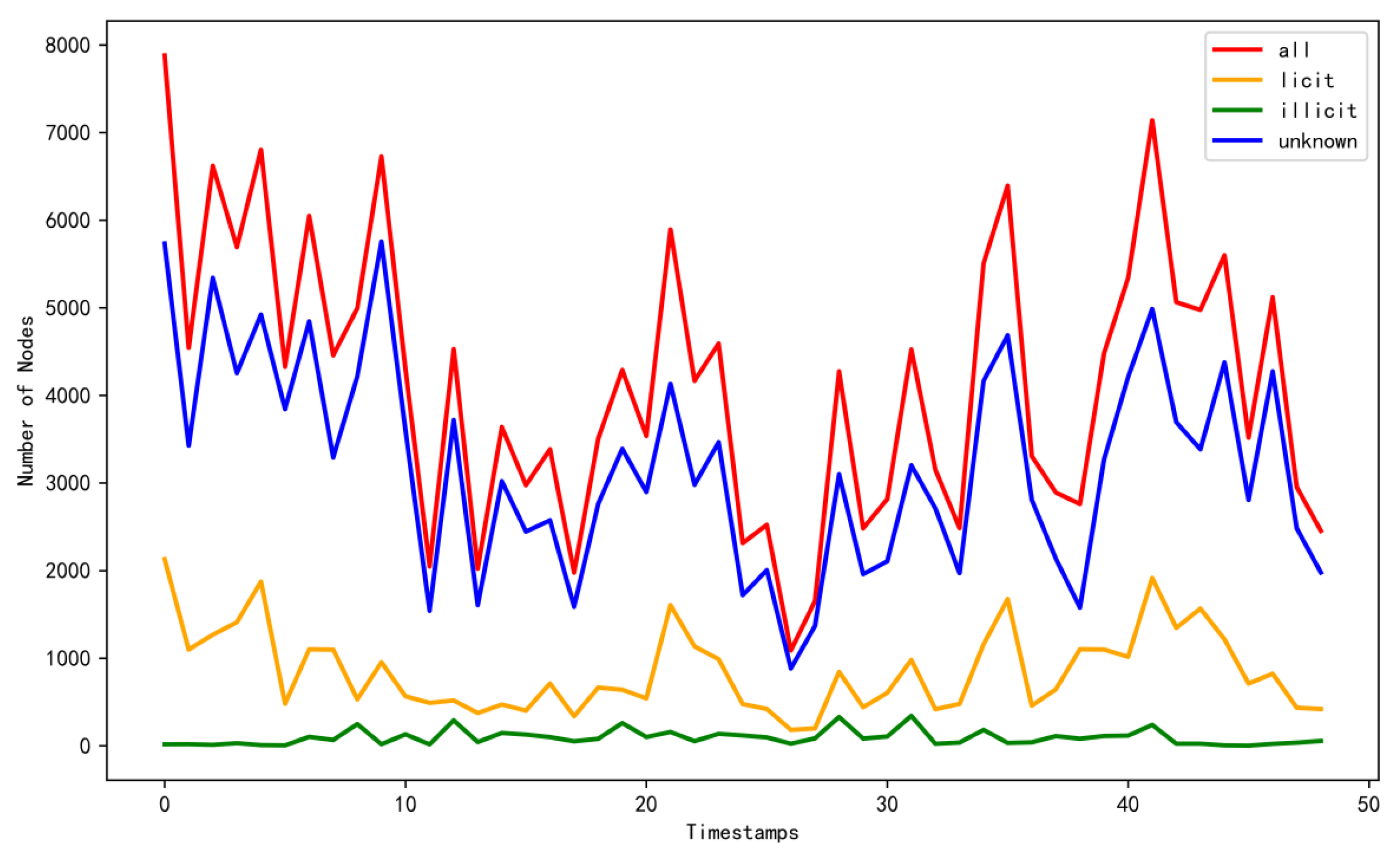
4.1.1. Description of the Dataset
4.1.2. Evaluation Metric Selection
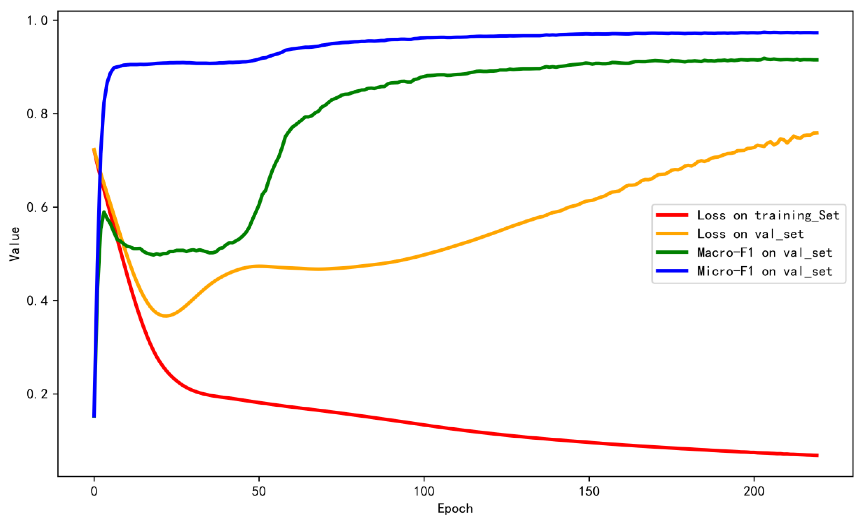
4.1.3. Model Parameter Selection
4.1.4. Baselines
4.2. Experimental Results and Analysis
4.3. Model Parameter Comparison and Analysis
4.3.1. Impact of the Graph Convolutional Layer Depth
4.3.2. Impact of Graph Convolutional Dropout
4.3.3. Impact of the Weight Decay Coefficient
5. Conclusions
Author Contributions
Funding
Data Availability Statement
Conflicts of Interest
References
- Korejo, M.S.; Rajamanickam, R.; Said, M.H.M. The concept of money laundering: A quest for legal definition. J. Money Laund. Control 2021, 24, 725–736. [Google Scholar] [CrossRef]
- Idowu, A.; Obasan, K.A. Anti-money laundering policy and its effects on bank performance in Nigeria. Bus. Intell. J. 2012, 5, 367–373. [Google Scholar]
- Gomber, P.; Kauffman, R.J.; Parker, C.; Weber, B.W. On the fintech revolution: Interpreting the forces of innovation, disruption, and transformation in financial services. J. Manag. Inf. Syst. 2018, 35, 220–265. [Google Scholar] [CrossRef]
- Awotunde, J.B.; Adeniyi, E.A.; Ogundokun, R.O.; Ayo, F.E. Application of big data with fintech in financial services. In Fintech with Artificial Intelligence, Big Data, and Blockchain; Springer: Singapore, 2021; pp. 107–132. [Google Scholar] [CrossRef]
- Juels, A.; Kosba, A.; Shi, E. The ring of gyges: Using smart contracts for crime. Aries 2015, 40, 54. [Google Scholar]
- Dyntu, V.; Dykyi, O. Cryptocurrency in the system of money laundering. Balt. J. Econ. Stud. 2018, 4, 75–81. [Google Scholar] [CrossRef]
- Bouri, E.; Lau, C.K.M.; Lucey, B.; David, R. Trading volume and the predictability of return and volatility in the cryptocurrency market. Financ. Res. Lett. 2019, 29, 340–346. [Google Scholar] [CrossRef]
- Chen, Z.; Khoa, L.D.V.; Teoh, E.N.; Nazir, A.; Karuppiah, E.K.; Lam, K.S. Machine learning techniques for anti-money laundering (AML) solutions in suspicious transaction detection: A review. Knowl. Inf. Syst. 2018, 57, 245–285. [Google Scholar] [CrossRef]
- Zhamiyeva, R.M.; Sultanbekova, G.B.; Abzalbekova, M.T.; Zhakupov, B.A.; Kozhanov, M.G. The role of financial investigations in combating money laundering. Int. J. Electron. Secur. Digit. Forensics 2022, 14, 188–198. [Google Scholar] [CrossRef]
- Ai, L. “Rule-based but risk-oriented” approach for combating money laundering in Chinese financial sectors. J. Money Laund. Control 2012, 15, 198–209. [Google Scholar] [CrossRef]
- Lokanan, M.E. Data mining for statistical analysis of money laundering transactions. J. Money Laund. Control 2019, 22, 753–763. [Google Scholar] [CrossRef]
- Liu, X.; Zhang, P. A scan statistics based suspicious transactions detection model for anti-money laundering (AML) in financial institutions. In Proceedings of the 2010 International Conference on Multimedia Communications, Hong Kong, China, 7–8 August 2010; pp. 210–213. [Google Scholar] [CrossRef]
- Levchenko, V.; Boyko, A.; Bozhenko, V.; Mynenko, S. Money laundering risk in developing and transitive economies: Analysis of cyclic component of time series. Verslas Teor. Ir Prakt./Bus. Theory Pract. 2019, 20, 492–508. [Google Scholar] [CrossRef]
- Gao, Z.; Ye, M. A framework for data mining-based anti-money laundering research. J. Money Laund. Control 2007, 10, 170–179. [Google Scholar] [CrossRef]
- Xia, P.; Ni, Z.; Zhu, X.; He, Q.; Chen, Q. A novel prediction model based on long short-term memory optimised by dynamic evolutionary glowworm swarm optimisation for money laundering risk. Int. J. Bio-Inspired Comput. 2022, 19, 77–86. [Google Scholar] [CrossRef]
- Weber, M.; Domeniconi, G.; Chen, J.; Weidele, D.K.I.; Bellei, C.; Robinson, T.; Leiserson, C.E. Anti-money laundering in bitcoin: Experimenting with graph convolutional networks for financial forensics. arXiv 2019, arXiv:1908.02591. [Google Scholar] [CrossRef]
- Weber, M.; Chen, J.; Suzumura, T.; Pareja, A.; Ma, T.; Kanezashi, H.; Kaler, T.; Leiserson, C.E.; Schardl, T.B. Scalable graph learning for anti-money laundering: A first look. arXiv 2018, 295, 18–32. [Google Scholar] [CrossRef]
- Pambudi, B.N.; Hidayah, I.; Fauziati, S. Improving money laundering detection using optimized support vector machine. In Proceedings of the 2019 International Seminar on Research of Information Technology and Intelligent Systems (ISRITI), Yogyakarta, Indonesia, 5–6 December 2019; pp. 273–278. [Google Scholar] [CrossRef]
- Chen, M.R.; Chen, B.P.; Zeng, G.Q. An adaptive fractional order BP neural network based on extremal optimization for handwritten digits recognition. Neurocomputing 2020, 391, 260–272. [Google Scholar] [CrossRef]
- Jiang, S.; Fengli, Z. Analysis and Prediction of E-Bank Suspicious Accounts Based on Ensemble Learning Under Imbalance Data. Int. Conf. Comput. Financ. Bus. Anal. 2023, 32, 231–242. [Google Scholar]
- Khokhsarai, H.M.; Shahriari, M.; Rudpashti, F.R.; Jaghargh, S.A.S. Presenting a methodology based on the self-organizing maps and multi-layer neural networks for suspected money laundering events at bank branches. J. New Res. Math. 2022, 8, 83–100. [Google Scholar] [CrossRef]
- Wang, S.; Liu, C.; Gao, X.; Qu, H.; Xu, W. Session-based fraud detection in online e-commerce transactions using recurrent neural networks. In Machine Learning and Knowledge Discovery in Databases (Lecture Notes in Computer Science); Springer: Cham, Switzerland, 2017; pp. 241–252. [Google Scholar] [CrossRef]
- Hochreiter, S.; Schmidhuber, J. Long short-term memory. Neural Comput. 1997, 9, 1735–1780. [Google Scholar] [CrossRef]
- Alghofaili, Y.; Albattah, A.; Rassam, M.A. A financial fraud detection model based on LSTM deep learning technique. J. Appl. Secur. Res. 2020, 15, 498–516. [Google Scholar] [CrossRef]
- Zhang, Y.; Yan, B.; Aasma, M. A novel deep learning framework: Prediction and analysis of financial time series using CEEMD and LSTM. Expert Syst. Appl. 2020, 159, 113609. [Google Scholar] [CrossRef]
- Chung, J.; Gulcehre, C.; Cho, K.H.; Bengio, Y. Empirical evaluation of gated recurrent neural networks on sequence modeling. arXiv 2014, arXiv:1412.3555. [Google Scholar] [CrossRef]
- Luo, S.; Ni, Z.; Zhu, X.; Xia, P.; Wu, H. A novel methanol futures price prediction method based on multicycle CNN-GRU and attention mechanism. Arab. J. Sci. Eng. 2023, 48, 1487–1501. [Google Scholar] [CrossRef]
- Labanca, D.; Primerano, L.; Markland-Montgomery, M.; Polino, M.; Carminati, M.; Zanero, S. Amaretto: An active learning framework for money laundering detection. IEEE Access 2022, 10, 41720–41739. [Google Scholar] [CrossRef]
- Alarab, I.; Prakoonwit, S.; Nacer, M.I. Competence of graph convolutional networks for anti-money laundering in bitcoin blockchain. In Proceedings of the 2020 5th International Conference on Machine Learning Technologies, Beijing, China, 19–21 June 2020; pp. 23–27. [Google Scholar] [CrossRef]
- You, J.; Gomes-Selman, J.M.; Ying, R.; Leskovec, J. Identity-aware Graph Neural Networks. Proc. AAAI Conf. Artif. Intell. 2021, 35, 10737–10745. [Google Scholar] [CrossRef]
- Li, G.; Muller, M.; Qian, G.; Perez, I.C.D.; Abualshour, A.; Thabet, A.K.; Ghanem, B. Deepgcns: Making gcns go as deep as cnns. IEEE Trans. Pattern Anal. Mach. Intell. 2021, 45, 6923–6939. [Google Scholar] [CrossRef]
- Mohan, A.; Karthika, P.V.; Sankar, P.; Manohar, M.; Peter, A. Improving anti-money laundering in bitcoin using evolving graph convolutions and deep neural decision forest. Data Technol. Appl. 2022, 57, 313–329. [Google Scholar] [CrossRef]
- Xia, P.; Ni, Z.; Xiao, H.; Zhu, X.; Peng, P. A novel spatiotemporal prediction approach based on graph convolution neural networks and long short-term memory for money laundering fraud. Arab. J. Sci. Eng. 2022, 47, 1921–1937. [Google Scholar] [CrossRef]
- Alarab, I.; Prakoonwit, S. Graph-based lstm for anti-money laundering: Experimenting temporal graph convolutional network with bitcoin data. Neural Process. Lett. 2023, 55, 689–707. [Google Scholar] [CrossRef]
- Jia, B.; Wang, C.; Zhao, H.; Shi, L. An Entity Linking Algorithm Derived from Graph Convolutional Network and Contextualized Semantic Relevance. Symmetry 2022, 14, 2060. [Google Scholar] [CrossRef]
- Yang, W.; Zhang, J.; Cai, J.; Xu, Z. Relation Selective Graph Convolutional Network for Skeleton-Based Action Recognition. Symmetry 2021, 13, 2275. [Google Scholar] [CrossRef]
- You, J.; Du, T.; Leskovec, J. ROLAND: Graph learning framework for dynamic graphs. In Proceedings of the 28th ACM SIGKDD Conference on Knowledge Discovery and Data Mining, Washington, DC, USA, 14–18 August 2022; pp. 2358–2366. [Google Scholar] [CrossRef]
- Zhu, J.; Li, B.; Zhang, Z.; Zhao, L.; Li, H. High-Order Topology-Enhanced Graph Convolutional Networks for Dynamic Graphs. Symmetry 2022, 14, 2218. [Google Scholar] [CrossRef]
- Vaswani, A.; Shazeer, N.; Parmar, N.; Uszkoreit, J.; Jones, L.; Gomez, A.N.; Kaiser, L.; Polosukhin, I. Attention is all you need. In Proceedings of the 2017 Neural Information Processing Systems, Long Beach, CA, USA, 4–9 December 2017; pp. 5998–6008. [Google Scholar]
- Tatulli, M.P.; Paladini, T.; D’Onghia, M.; Carminati, M.; Zanero, S. HAMLET: A Transformer Based Approach for Money Laundering Detection. In Proceedings of the International Symposium on Cyber Security, Cryptology, and Machine Learning, Beer Sheva, Israel, 29–30 June 2023; pp. 234–250. [Google Scholar]
- Huang, H.; Wang, P.; Zhang, Z.; Zhao, Q. A Spatio-Temporal Attention-Based GCN for Anti-money Laundering Transaction Detection. In International Conference on Advanced Data Mining and Applications; Springer: Cham, Switzerland, 2023; pp. 634–648. [Google Scholar] [CrossRef]
- Peng, H.; Wang, H.; Du, B.; Bhuiyan, M.Z.A.; Ma, H.; Liu, J.; Wang, L.; Yang, Z.; Du, L.; Wang, S.; et al. Spatial temporal incidence dynamic graph neural networks for traffic flow forecasting. Inf. Sci. 2020, 521, 277–290. [Google Scholar] [CrossRef]
- Wang, X.; Ma, Y.; Wang, Y.; Jin, W.; Wang, X.; Tang, J.; Jia, C.; Yu, J. Traffic flow prediction via spatial temporal graph neural network. In Proceedings of the Web Conference 2020, Taipei, Taiwan, 20–24 April 2020; pp. 1082–1092. [Google Scholar] [CrossRef]
- Yu, B.; Yin, H.; Zhu, Z. Spatio-temporal graph convolutional networks: A deep learning framework for traffic forecasting. In Proceedings of the Twenty-Seventh International Joint Conference on Artificial Intelligence, Stockholm, Sweden, 13–19 July 2018; pp. 3634–3640. [Google Scholar] [CrossRef]
- Hu, W.; Fey, M.; Zitnik, M.; Dong, Y.; Ren, H.; Liu, B.; Catasta, M.; Leskovec, J. Open graph benchmark: Datasets for machine learning on graphs. Adv. Neural Inf. Process. Syst. 2020, 33, 22118–22133. [Google Scholar] [CrossRef]
- Wang, M.Y. Deep graph library: Towards efficient and scalable deep learning on graphs. In Proceedings of the ICLR Workshop on Representation Learning on Graphs and Manifolds, New Orleans, LA, USA, 6 May 2019. [Google Scholar]
- Ahmed, A. Anti-money laundering recognition through the gradient boosting classifier. Acad. Account. Financ. Stud. J. 2021, 25, 1–11. [Google Scholar]
- Zhang, Y.; Yu, W.; Li, Z.; Raza, S.; Cao, H. Detecting ethereum Ponzi schemes based on improved LightGBM algorithm. IEEE Trans. Comput. Soc. Syst. 2021, 9, 624–637. [Google Scholar] [CrossRef]
- Chen, D.; Lin, Y.; Li, W.; Li, P.; Zhou, J.; Sun, X. Measuring and relieving the over-smoothing problem for graph neural networks from the topological view. Proc. AAAI Conf. Artif. Intell. 2020, 34, 3438–3445. [Google Scholar] [CrossRef]


| Dataset | Categories | Timestamps | Feature Dimensions | Nodes | Edges |
|---|---|---|---|---|---|
| Elliptic | 2 | 49 | 166 | 203,769 | 234,355 |
| OGB-Arxiv | 40 | 41 | 129 | 169,343 | 1,166,243 |
| Parameter | Value |
|---|---|
| Training set proportion | 80% |
| Validation set proportion | 10% |
| Test set proportion | 10% |
| RNN_layers | 2 |
| Graph_layers | 2 |
| Support | 2 |
| Training epochs | 220 |
| Lr | 0.001 |
| Loss function | Cross entropy |
| Optimizer | Adam |
| Weight_decay | 5 × 10⁻⁵ |
| Activation function | ReLU |
| Dataset | Model | Micro-Precision | Micro-Recall | Micro-F1 | Macro-Precision | Macro-Recall | Macro-F1 | Ex-Time(s) |
|---|---|---|---|---|---|---|---|---|
| Elliptic | GRU | 0.9345 | 0.9345 | 0.9345 | 0.8670 | 0.6937 | 0.7474 | 12.58 |
| LSTM | 0.9364 | 0.9364 | 0.9364 | 0.8651 | 0.7104 | 0.7619 | 14.50 | |
| GCN | 0.9192 | 0.9192 | 0.9192 | 0.7596 | 0.8173 | 0.7844 | 14.73 | |
| GCN-GRU | 0.9310 | 0.9310 | 0.9310 | 0.7927 | 0.8103 | 0.8012 | 30.50 | |
| MGC-LSTM | 0.9351 | 0.9351 | 0.9351 | 0.8107 | 0.7938 | 0.8019 | 32.95 | |
| DGCN-GRU | 0.9360 | 0.9360 | 0.9360 | 0.8096 | 0.8109 | 0.8103 | 27.20 | |
| MDGC-LSTM | 0.9435 | 0.9435 | 0.9435 | 0.8380 | 0.8161 | 0.8266 | 30.34 |
| Dataset | Model | Micro-Precision | Micro-Recall | Micro-F1 | Macro-Precision | Macro-Recall | Macro-F1 | Ex-Time(s) |
|---|---|---|---|---|---|---|---|---|
| OGB- Arxiv | GRU | 0.2814 | 0.2435 | 0.2331 | 0.2814 | 0.2435 | 0.2331 | 71.08 |
| LSTM | 0.2747 | 0.2434 | 0.2398 | 0.2747 | 0.2434 | 0.2398 | 92.41 | |
| GCN | 0.2992 | 0.2495 | 0.2476 | 0.2992 | 0.2495 | 0.2476 | 94.66 | |
| GCN-GRU | 0.3635 | 0.2589 | 0.2708 | 0.3635 | 0.2589 | 0.2708 | 175.69 | |
| MGC-LSTM | 0.3536 | 0.2675 | 0.2804 | 0.3536 | 0.2675 | 0.2804 | 209.18 | |
| DGCN-GRU | 0.3157 | 0.3011 | 0.2988 | 0.3157 | 0.3011 | 0.2988 | 162.05 | |
| MDGC-LSTM | 0.3414 | 0.3131 | 0.3169 | 0.3414 | 0.3131 | 0.3169 | 202.43 |
| Dataset | Model | Micro-Precision | Micro-Recall | Micro-F1 | Macro-Precision | Macro-Recall | Macro-F1 | Ex-Time(s) |
|---|---|---|---|---|---|---|---|---|
| Elliptic | LR | 0.9338 | 0.9338 | 0.9338 | 0.8356 | 0.7372 | 0.7755 | 0.24 |
| SVM | 0.9540 | 0.9540 | 0.9540 | 0.9758 | 0.7584 | 0.8283 | 4893 | |
| RF | 0.9531 | 0.9531 | 0.9531 | 0.9691 | 0.7558 | 0.8247 | 0.34 | |
| BP | 0.9596 | 0.9596 | 0.9596 | 0.9231 | 0.8282 | 0.8681 | 3.96 | |
| XGBoost | 0.9600 | 0.9600 | 0.9600 | 0.9119 | 0.8419 | 0.8728 | 0.38 | |
| LightGBM | 0.9598 | 0.9598 | 0.9598 | 0.9099 | 0.8428 | 0.8725 | 0.45 | |
| MDGC-LSTM | 0.9742 | 0.9742 | 0.9742 | 0.9491 | 0.8922 | 0.9183 | 30.34 |
| Dataset | Model | Micro-Precision | Micro-Recall | Micro-F1 | Macro-Precision | Macro-Recall | Macro-F1 | Ex-Time(s) |
|---|---|---|---|---|---|---|---|---|
| OGB-Arxiv | LR | 0.4102 | 0.4102 | 0.4102 | 0.1344 | 0.1104 | 0.0974 | 1.12 |
| SVM | 0.2759 | 0.2759 | 0.2759 | 0.4013 | 0.1061 | 0.1351 | 26084 | |
| RF | 0.2441 | 0.2441 | 0.2441 | 0.1855 | 0.2575 | 0.1687 | 1.77 | |
| BP | 0.4425 | 0.4425 | 0.4425 | 0.2814 | 0.2435 | 0.2331 | 21.72 | |
| XGBoost | 0.3482 | 0.3482 | 0.3482 | 0.1888 | 0.1069 | 0.1095 | 1.92 | |
| LightGBM | 0.2701 | 0.2701 | 0.2701 | 0.2018 | 0.2824 | 0.1873 | 2.61 | |
| MDGC-LSTM | 0.5629 | 0.5629 | 0.5629 | 0.4202 | 0.3486 | 0.3715 | 202.43 |
Disclaimer/Publisher’s Note: The statements, opinions and data contained in all publications are solely those of the individual author(s) and contributor(s) and not of MDPI and/or the editor(s). MDPI and/or the editor(s) disclaim responsibility for any injury to people or property resulting from any ideas, methods, instructions or products referred to in the content. |
© 2024 by the authors. Licensee MDPI, Basel, Switzerland. This article is an open access article distributed under the terms and conditions of the Creative Commons Attribution (CC BY) license (https://creativecommons.org/licenses/by/4.0/).
Share and Cite
Wan, F.; Li, P. A Novel Money Laundering Prediction Model Based on a Dynamic Graph Convolutional Neural Network and Long Short-Term Memory. Symmetry 2024, 16, 378. https://doi.org/10.3390/sym16030378
Wan F, Li P. A Novel Money Laundering Prediction Model Based on a Dynamic Graph Convolutional Neural Network and Long Short-Term Memory. Symmetry. 2024; 16(3):378. https://doi.org/10.3390/sym16030378
Chicago/Turabian StyleWan, Fei, and Ping Li. 2024. "A Novel Money Laundering Prediction Model Based on a Dynamic Graph Convolutional Neural Network and Long Short-Term Memory" Symmetry 16, no. 3: 378. https://doi.org/10.3390/sym16030378
APA StyleWan, F., & Li, P. (2024). A Novel Money Laundering Prediction Model Based on a Dynamic Graph Convolutional Neural Network and Long Short-Term Memory. Symmetry, 16(3), 378. https://doi.org/10.3390/sym16030378