Abstract
Single-phase-to-ground fault in low-current grounding systems represents a serious public safety concern. Low-voltage (LV) sensors, with their growing maturity, can now monitor multiple points of the mid-voltage (MV) distribution network. This paper proposes a new method for identifying single-phase-to-ground line faults and locating them using LV sensors deployed on the LV side of distribution transformers. We analyze the characteristics of the negative-sequence signal on the LV side after a single-phase grounding fault occurs on the MV side. The negative-sequence current can distinguish between fault and non-fault lines. By setting the ratio coefficient of negative-sequence voltage and positive-sequence voltage, we can use multi-point collaborative calculation and comparison to determine the section of the fault point. We consider the unbalanced load on the LV side and the special case of a fault point on one end of the line. Through simulation of combined MV and LV distribution systems in MATLAB software and dynamic model experiments, we verify that the proposed method has good robustness and accuracy. Monitoring the status information of the MV distribution network through LV sensors has great potential in practical application and implementation for realizing the fault detection of low-current grounding systems.
1. Introduction
In China’s 3~10 kV distribution networks, the neutral point is often left ungrounded or grounded through arc suppression coils, which are also referred to as low-current grounding systems [1,2]. As a critical link connecting the power system with end users, the characteristics of distribution networks dictate their vulnerability to external factors and internal equipment issues, rendering them more susceptible to faults compared to transmission networks. Single-phase grounding faults are prevalent in low-current grounding systems, constituting over 80% of the distribution network fault rate. During faults, voltages in non-fault phases increase, posing risks to the insulation of the power grid and the safe operation of electrical equipment. Moreover, faults can lead to electric shock accidents, resulting in injuries and fatalities, with single-phase electric shock accidents comprising over 70% of all electric shock incidents. In recent years, power companies have increasingly recognized the significance of this issue [3,4]. Hence, rapid, efficient, and precise fault detection methods are imperative for identifying faulted lines and promptly confirming fault section locations, enabling maintenance personnel to address issues promptly [5,6].
In the current widespread application of low-current grounding systems, the fault detection and discrimination of faulty lines are of significant importance for enhancing the reliability of power system operation and effectively maintaining the safety of grid equipment. However, due to the indistinct characteristics of single-phase grounding faults in low-current grounding systems, fault detection remains a recognized industry challenge [7]. Over the years, numerous scholars have conducted extensive research and proposed many methods for detecting low-current grounding faults and determining faulty lines. These methods can be categorized into steady-state methods and transient methods. Steady-state methods include specific techniques such as the zero-sequence admittance method, zero-sequence current amplitude ratio phase method, zero-sequence current active component method, negative-sequence current method, and harmonic method [8,9,10,11]. These methods offer advantages such as clear fault characteristic quantities and stable signal acquisition. Unlike steady-state methods, transient methods provide rich transient information and distinct local features but have poor disturbance resistance. They include traditional energy methods, inherent modal energy methods, wavelet analysis methods, and correlation analysis methods [12,13,14,15,16]. However, due to economic considerations, only a small number of fault detection devices are typically installed on the mid-voltage (MV) side at substations or along lines, and sometimes their actual performance is not satisfactory. Power companies are forced to resort to traditional methods such as fault location through line patrolling, leading to interruptions in power supply to non-faulty lines and affecting power quality, resulting in the abnormal operation of sensitive electrical equipment [17]. Therefore, power companies urgently need to improve the accuracy of low-current system grounding fault detection and enhance the safety and reliability of low-current system operation, without adding too many additional devices so that economic requirements can be met [18].
In recent years, there has been rapid progress in the construction of distribution Internet of Things (IoT), especially the widespread deployment of smart distribution transformer terminals. These smart terminals, installed on the low-voltage (LV) side of each distribution transformer, maintain network time synchronization with cloud-based main stations through broadband carrier waves, low-power wireless communication, and other means. This enables power companies to have comprehensive situational awareness of the distribution network throughout the system. By using measurement data from the low-voltage side, some local faults can be detected, thereby enhancing the management and control of the low-voltage distribution network [19]. Additionally, it brings new solutions to the challenge of detecting low-current grounding faults on the MV side of the system. In this paper, we analyze the monitoring signals from the smart distribution transformer terminals installed on the LV side of distribution transformers. We extract and identify the negative-sequence current on the MV side of the distribution network after a fault occurs. By comparing multiple sensing signals, our method uses the magnitude of the negative-sequence current to determine the faulty lines. Furthermore, it utilizes the ratio coefficient of negative-sequence voltage to positive-sequence voltage for multi-point collaborative determination of the fault section position. Special considerations are given to cases of unbalanced loads on the LV side and faults occurring at one end of the line.
The proposed method, utilizing measurement data from the installed smart terminals on the LV side, serves as an auxiliary means for monitoring on the MV side. It effectively addresses the problem of fault identification and section localization in low-current systems, thereby enhancing the fault-management capabilities of the MV distribution network. This approach ensures both economic efficiency and system safety while safeguarding equipment and personal safety.
2. LV-Side Perception Analysis
2.1. Characteristics of Negative-Sequence Current in Fault Lines
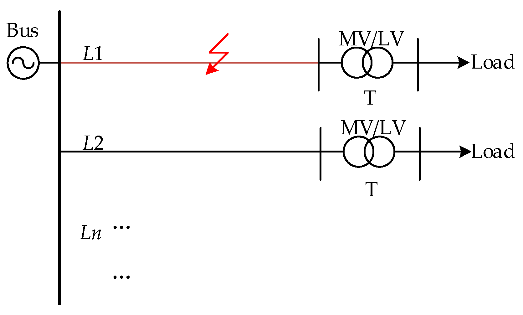
In low-current grounding systems, the equivalent circuits for zero sequence vary depending on the grounding method at the system’s neutral point. Consequently, the distribution of zero-sequence current changes with variations in the grounding method. However, the equivalent circuit for the negative sequence remains unaffected by changes in the neutral-point grounding method. Neither Δ/Y nor Y/Y connection winding configurations impede the flow of negative-sequence quantities. Additionally, signals within the 3 kHz range can be transmitted to the LV side without accounting for errors introduced by transformer conversion [20,21]. Further analysis of the characteristics of negative-sequence quantities in the system depicted in Figure 1 is presented in the following.

Figure 1.
Diagram of topology of system.
The system depicted in Figure 1 includes multiple MV lines (L1–Ln), with smart terminals installed on the LV side of distribution transformers. In the event of a single-phase grounding fault occurring on line L1, the distribution of negative-sequence current in the system can be illustrated by the equivalent circuit shown in Figure 2.
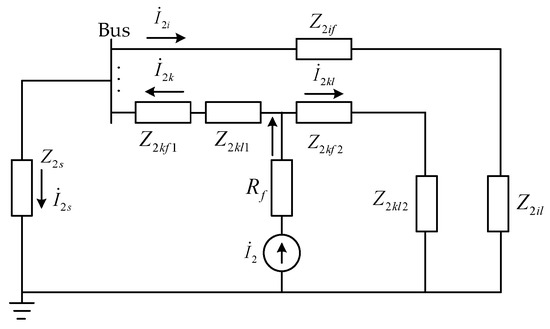
Figure 2.
Negative-sequence current distribution of single-phase grounding fault.
In Figure 2, Rf represents the fault resistance, Z2s denotes the system’s negative-sequence impedance, Z2if stands for the negative-sequence impedance of normal line i, Z2kf1 represents the negative-sequence impedance from the bus to the fault point for the faulted line, Z2kf2 signifies the negative-sequence impedance for other parts of the faulted line, Z2il indicates the negative-sequence impedance of the load for the normal line, Z2kl1 represents the negative-sequence impedance from the fault point to the bus for line k, and Z2kl2 denotes the negative-sequence impedance for other parts of line k’s load.
The negative-sequence currents generated at the fault point flow, respectively, towards the power supply side and the load side. As shown in Figure 2,
In (1), represents the ratio of negative-sequence current flowing towards the non-fault line to that flowing towards the power source.
Due to the low conversion of the system’s high-voltage side negative-sequence impedance to the LV side [22] and the high impedance value of distribution network loads, which is typically tens to hundreds of times larger than the system’s negative-sequence impedance, we have the following:
Moreover, in urban areas, the length of distribution feeder lines typically ranges from 2 to 10 km, with the feeder line’s negative-sequence impedance significantly being smaller than the negative-sequence impedance of the load; therefore,
It is generally believed that K2 is less than 0.01 [22]. Hence, it can be concluded that
In summary, it is apparent that the negative-sequence current arising from single-phase grounding faults in low-current systems predominantly flows towards the power source upon reaching the bus. Conversely, the negative-sequence current directed towards non-fault lines is negligible. Consequently, by contrasting the magnitude of negative-sequence currents sensed on the LV side of feeder lines at the onset of the distribution area, discerning between faulty and non-faulty lines on the MV side becomes feasible.
2.2. Characteristics of Negative-Sequence Voltage Upstream and Downstream of the Fault Point
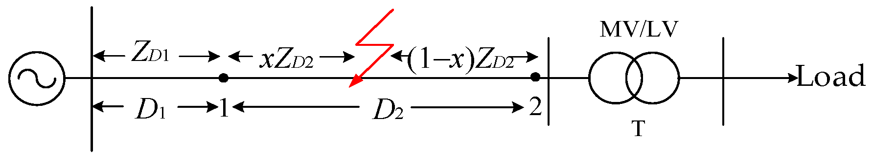
Once the faulty line is identified, further determination of the fault section location is made by analyzing the fault characteristics sensed on the LV side upstream and downstream of the fault point. By disregarding the non-faulty lines in Figure 1, the fault single-line diagram is obtained, as illustrated in Figure 3.
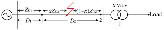
Figure 3.
Fault circuit diagram.
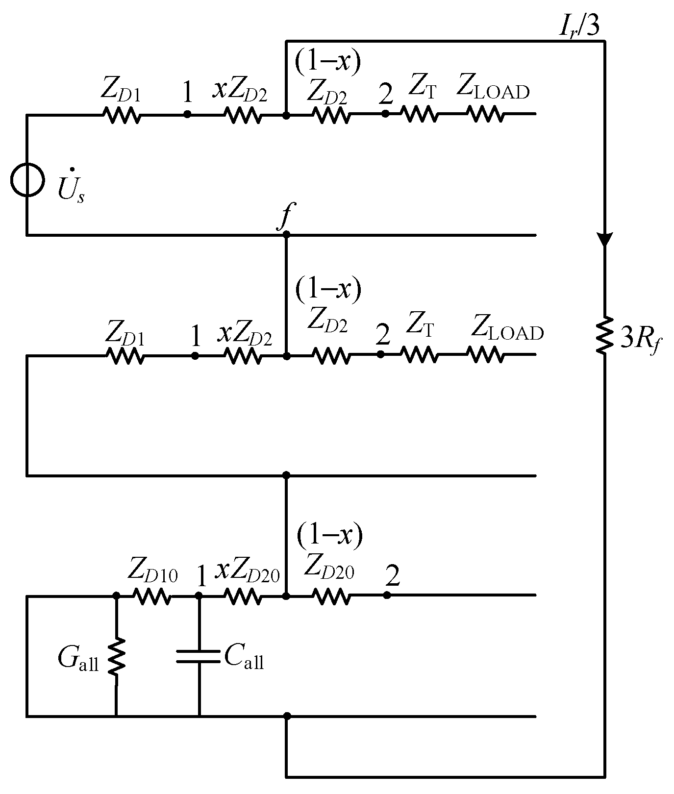
In Figure 3, the fault point is located between transformer 1 and transformer 2; the length from the busbar to transformer 1 is denoted as D1, with impedance ZD1 representing the line impedance. The length between transformer 1 and 2 is denoted as D2, with impedance ZD2 representing the line impedance. The fault point is situated at a position x along the length D2 from transformer 1. After the fault occurs, the system’s equivalent composite sequence network is depicted in Figure 4.
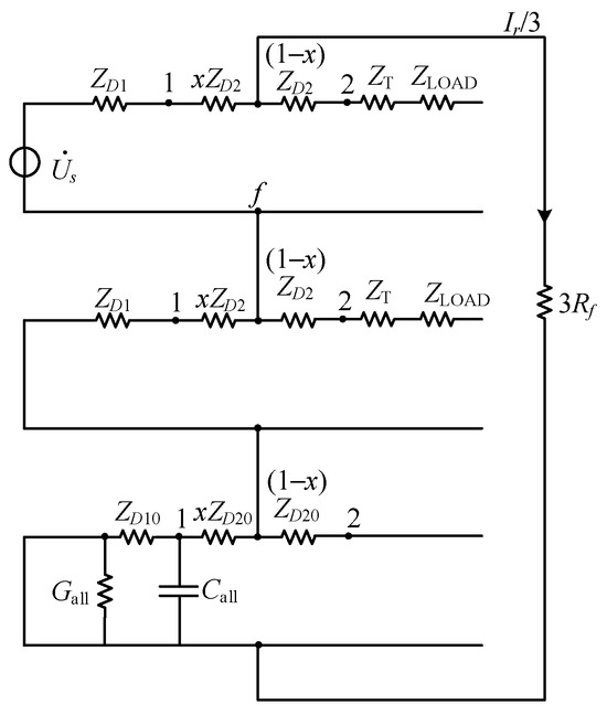
Figure 4.
Compound sequence network of single-phase grounding fault.
In Figure 4, Z10 and Z20 represent the line zero-sequence impedance, while Gall and Call, respectively, denote the total parallel conductance and capacitance to ground. If represents the fault current. From Equation (1), it can be inferred that the current flowing downstream from the fault point is minimal. Therefore, downstream of the fault point can be approximated as an open circuit [23,24]. Thus, the positive-sequence voltage Uf+, negative-sequence voltage Uf−, and zero-sequence voltage Uf0 at the fault point can be expressed as follows:
In the equation, Z0 represents the total zero-sequence impedance of the line. We introduce the coefficient ηf to represent the ratio of negative-sequence voltage to positive-sequence voltage at the fault point:
Similarly, the positive-sequence voltage Uf1+, negative-sequence voltage Uf1−, zero-sequence voltage Uf10, and coefficient ηf1 at point 1 upstream of the fault are expressed as follows:
Comparing Equation (6) with Equation (8), the relationship between the negative-sequence voltages at the fault point and upstream location 1 is Uf− > Uf1−. Similarly, the relationship between positive-sequence voltages is Uf+ < Uf1+, thus yielding ηf > ηf1 as the relationship between the coefficients at the fault point and upstream location 1. As deduced in Section 2.1, the current flowing downstream from the fault point is minimal, and therefore the voltage change downstream is approximately the same as at the fault point. Consequently, the relationship between the coefficients at the fault point and downstream location 2 can be approximated as ηf ≈ ηf2. Thus, the relationship between the coefficients at the fault point and upstream and downstream locations satisfies:
In conclusion, based on the relationship between the coefficient ratios of the fault point and upstream and downstream locations on the line, fault section localization between distribution areas along the line can be achieved through coordinated comparison at multiple points on the LV side.
3. Fault Detection Method
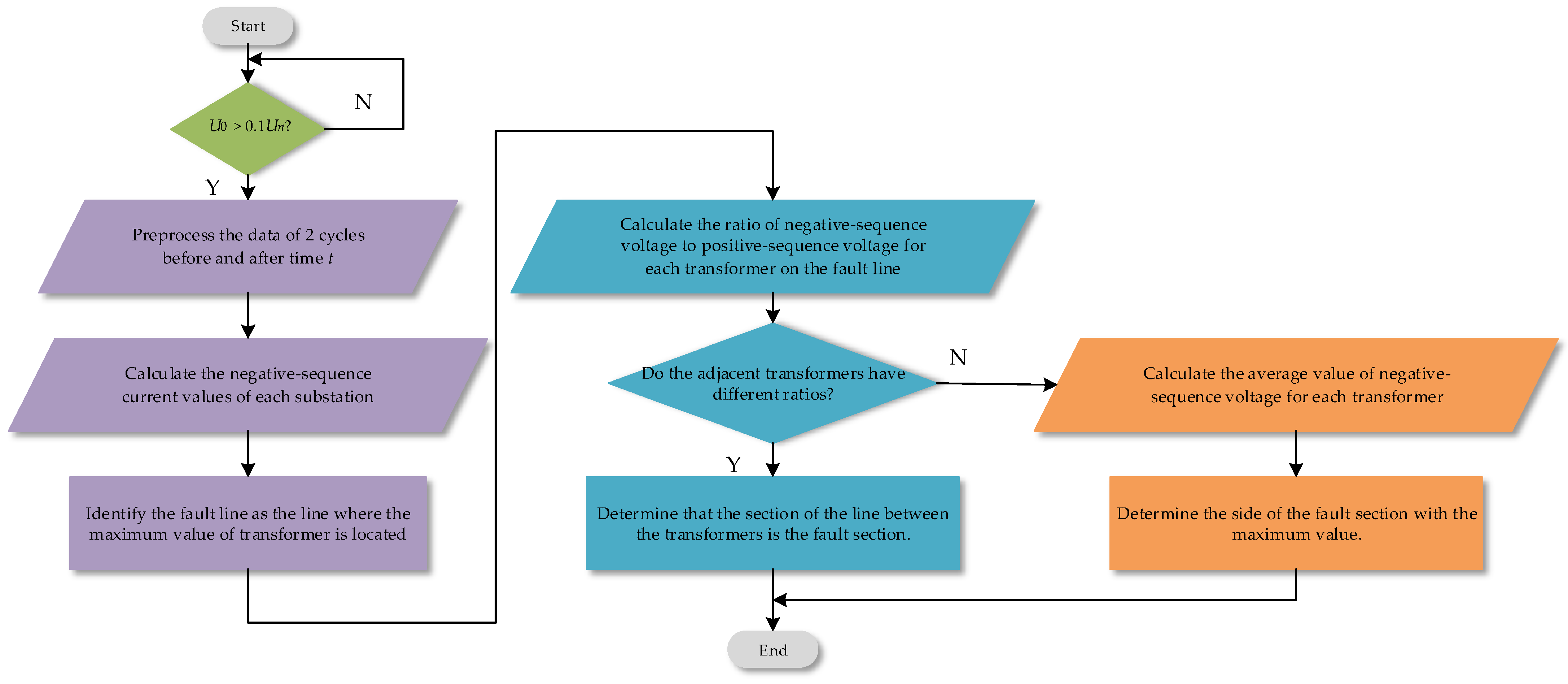
Based on the preceding analysis, it is apparent that in low-current systems, when a single-phase grounding fault occurs on the MV side, fault signal characteristics can be monitored on the LV side. To enhance the stability of the proposed method, it can be integrated with fault detection methods on the MV side. An activation criterion can be set, triggering when the abnormality of zero-sequence voltage detected on the MV side exceeds a preset threshold (typically set at 10% of the phase voltage, varying with system asymmetry), concurrently with abnormal changes in negative-sequence current detected on the LV side. Specifically, within two consecutive power frequency cycles, if the change in the negative-sequence current value on one line’s LV side is significantly greater than that of all other lines, it is considered that a single-phase grounding fault may have occurred, and this event is recorded at time t. The criteria for fault detection are illustrated in Figure 5.
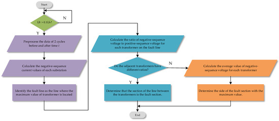
Figure 5.
Fault detection procedure.
Typically, the duration of asymmetrical loads on the LV side exceeds that of fault occurrences, warranting brief sampling times to minimize the impact of asymmetrical load fluctuations. Hence, data from each outgoing line’s terminal distribution area, spanning two power frequency cycles before and after time t, are selected as raw data. Preprocessing involves subtracting the mean value of the two cycles after time t from that of the two cycles before time t, effectively neutralizing the influence of asymmetrical loads on subsequent fault selection and localization. Subsequently, the line associated with the distribution area with the highest average value is identified as the faulty line.
After determining the faulty line, various LV measurement data from distribution areas along the faulty line are utilized to introduce the coefficient ratio η for determining the fault section location. This involves computing the ratio Pi (I = 1, …, n) of negative-sequence voltage to positive-sequence voltage for the n distribution areas on the fault line after preprocessing. Subsequently, clustering calculation is performed on Pi using Equation (9), aiming to divide them into two groups, Pi1 and Pi2, while maximizing inter-class variance and minimizing intra-class variance.
When a fault occurs at the beginning or end of a line, the coefficient ratio η for each distribution area along the line is approximately the same. Therefore, it is necessary to compare the magnitude of negative-sequence voltages to determine whether the distribution areas contained in Pi1 and Pi2 are located on either side of the fault section.
If correct, the line connecting Pi1 and Pi2 is designated as the fault section. If denied, the fault point should be at one end of the line. The average negative-sequence voltage of n distribution areas on the fault line is computed after preprocessing, and the distribution area with the highest average negative-sequence voltage is designated as the fault section.
4. Analysis of Simulation and Dynamic Model Experiment
4.1. Analysis of Simulation Results
4.1.1. Analysis of Faulty Line Selection Results
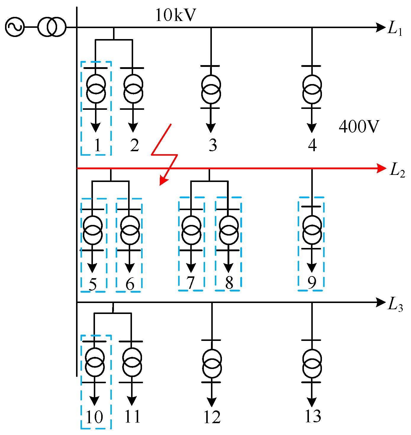
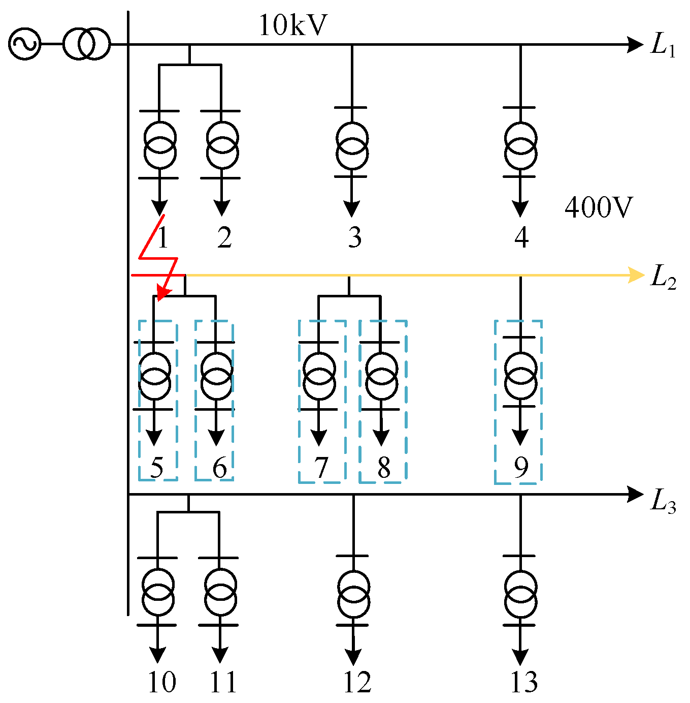
In SIMULINK, a simulation environment is constructed, comprising three 10 kV lines, L1, L2, and L3, along with a total of 13 LV distribution areas. The transformers in the distribution areas are all connected in ∆/Y configuration, with the system neutral point not grounded. Line L2 is chosen as the fault line, and the simulation system structure is shown in Figure 6.
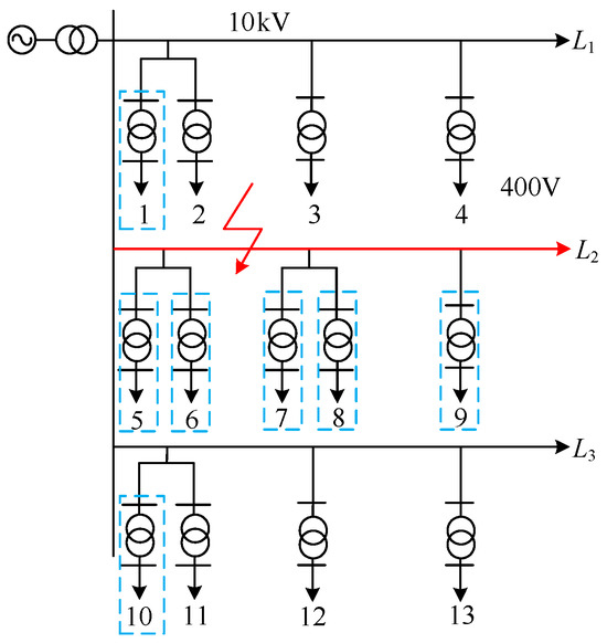
Figure 6.
Simulation system for fault line selection results.
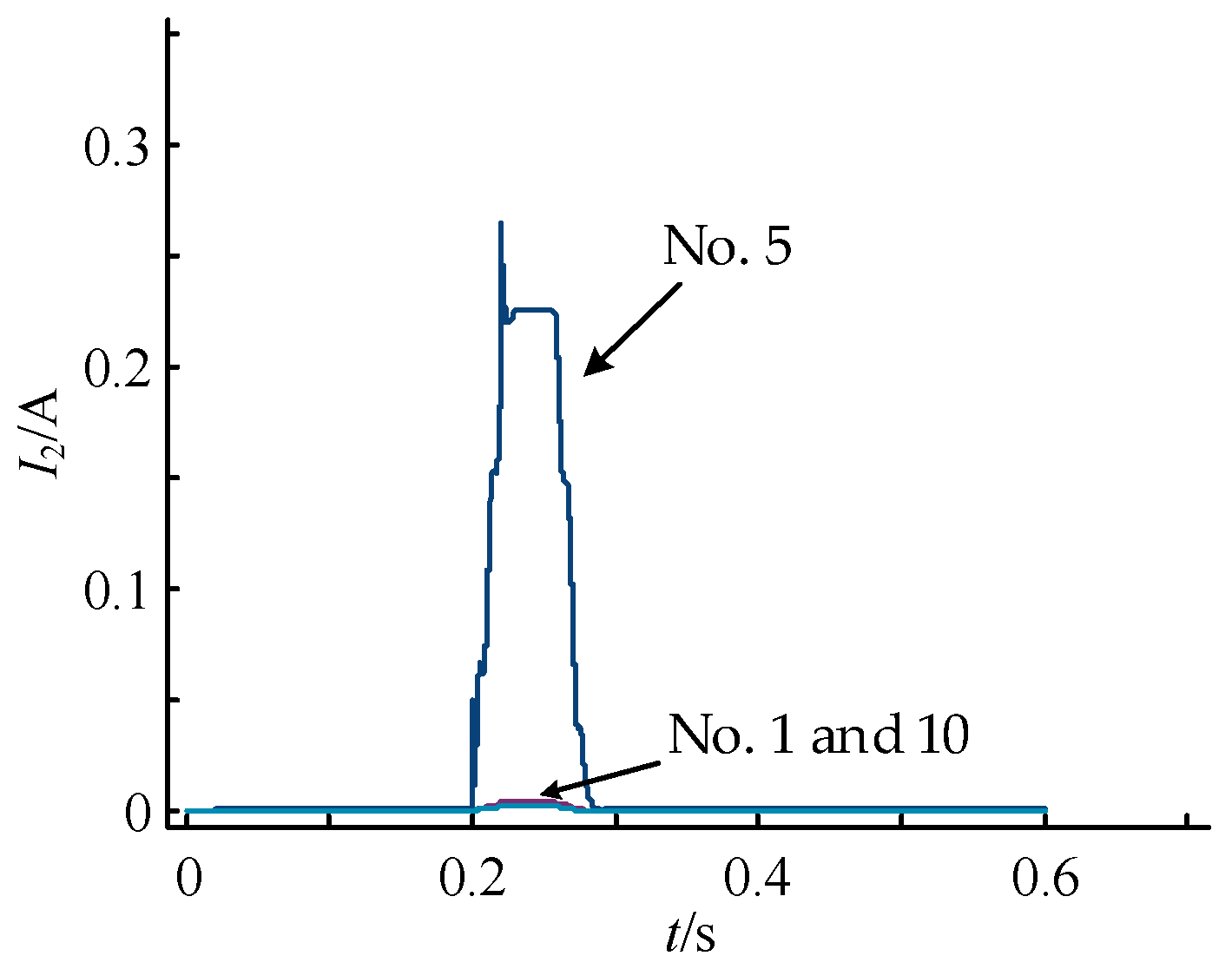
The single-phase-to-ground fault occurs at the power supply end of the 10 kV line, triggered at 0.2 s and recovered at 0.25 s, with a fault resistance value of 100 Ω. After the fault occurs, the comparison of the negative-sequence currents at the low-voltage ends of the L1, L2, and L3 lines is shown in Figure 7.
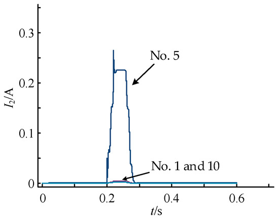
Figure 7.
Comparison of LV negative-sequence current values (No. 1, 5, and 10 transformers). Ground fault resistance: 100 Ω.
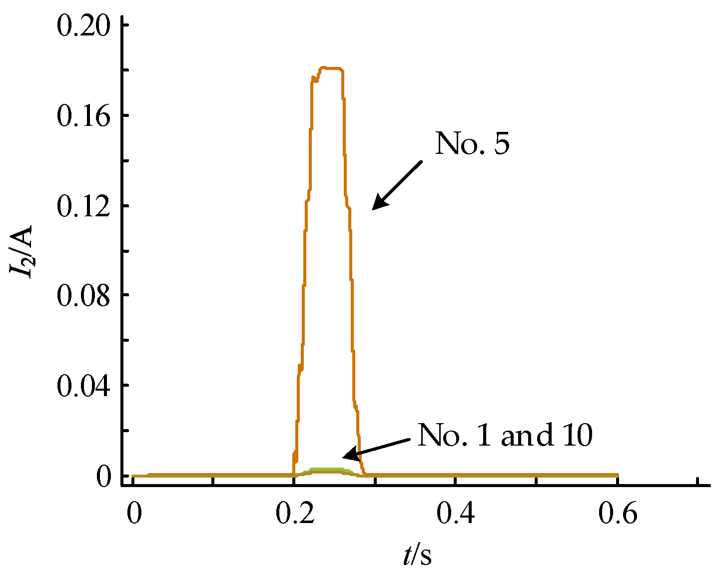
From Figure 7, it can be observed that the negative-sequence current at the LV end of transformer 5, which is at the fault line’s starting point, is significantly higher than that of transformers 1 and 10. This indicates that the negative-sequence current generated by the fault flows mostly towards the system side after reaching the bus, with very little flowing towards the non-faulted lines. In Figure 8, when the fault grounding resistance is increased to 2000 Ω, the negative-sequence current at the LV side decreases, but still maintains the relationship where the negative-sequence current at the fault line’s starting point is much higher than that of the non-faulted lines.
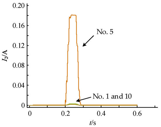
Figure 8.
Comparison of LV negative-sequence current values (No. 1, 5, and 10 transformers) upon increasing the fault grounding resistance to 2000 Ω.
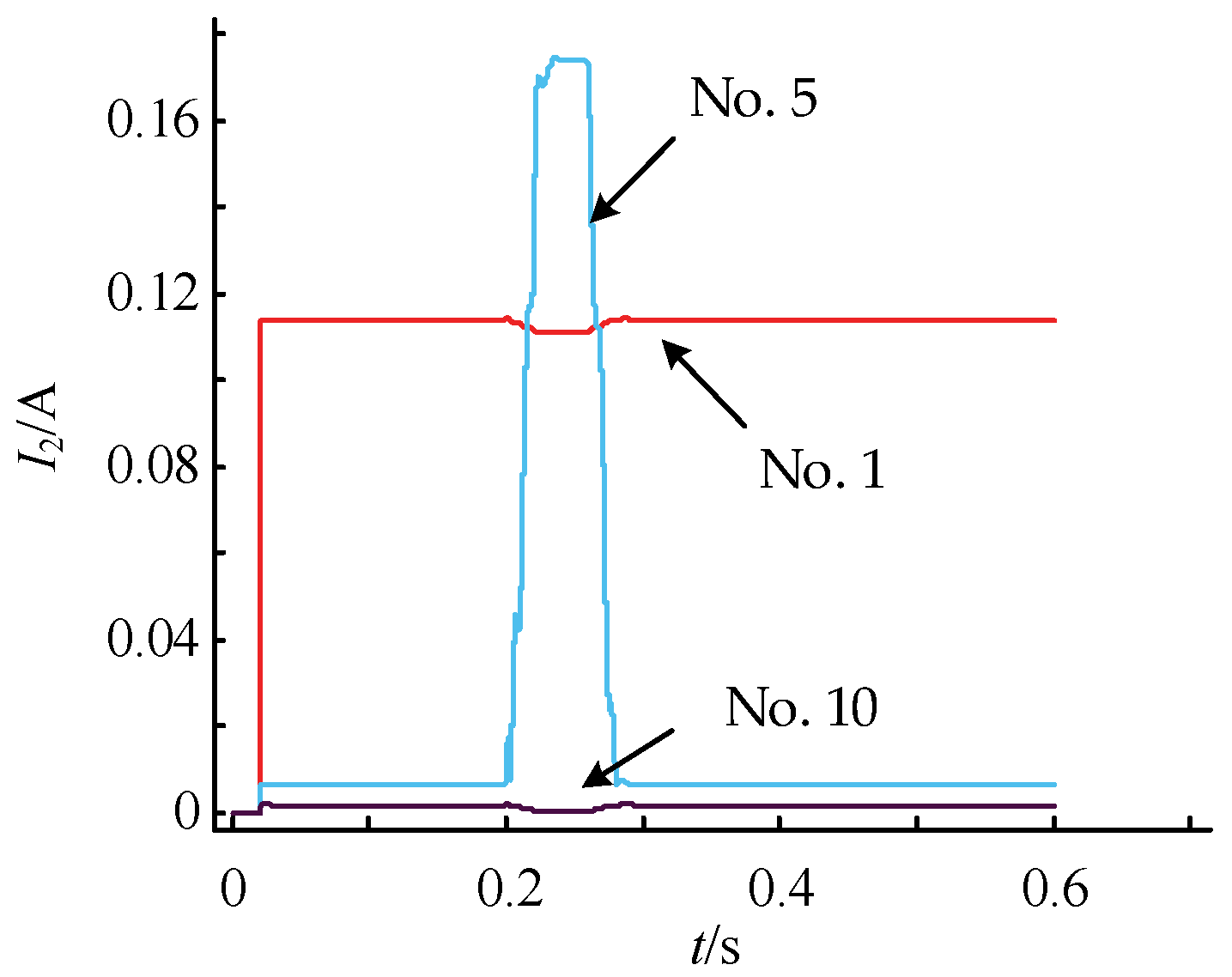
Considering the common factor of unbalanced operation on the LV side, the simulation results under three-phase unbalanced conditions are shown in Figure 9.
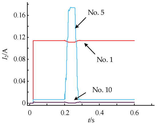
Figure 9.
Comparison of LV negative-sequence current values (No. 1, 5, and 10 transformers) for three-phase unbalanced operation.
The grounding fault resistance remains unchanged at 2000 Ω, with 20% three-phase imbalance in transformer 3 of non-fault line L1. Clear negative-sequence currents appear on the LV side of transformer 1 of the same line. Comparing the changes in negative-sequence currents caused by faults on the MV side, the negative-sequence currents generated by LV three-phase imbalance persist for a longer duration, with stable and almost constant amplitudes. Hence, averaging the values over two power-frequency cycles after 0.2 s and subtracting them from the averages over the preceding two cycles can eliminate the influence of three-phase imbalance on the analysis of negative-sequence currents.
4.1.2. Analysis of Fault Section Localization Results
After identifying the faulty line, the fault section location is determined by comparing the ratio of negative-sequence voltage to positive-sequence voltage on the LV side of each transformer along the faulty line. The simulation system is illustrated in Figure 10.
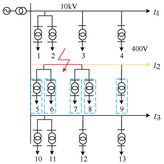
Figure 10.
Simulation system for fault section location results.
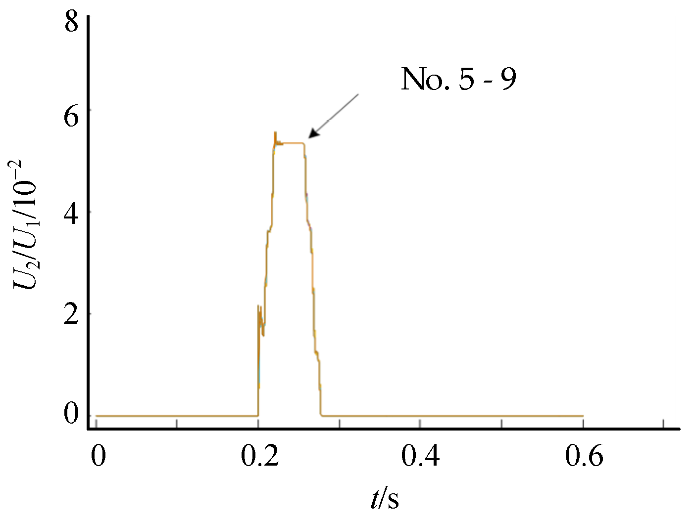
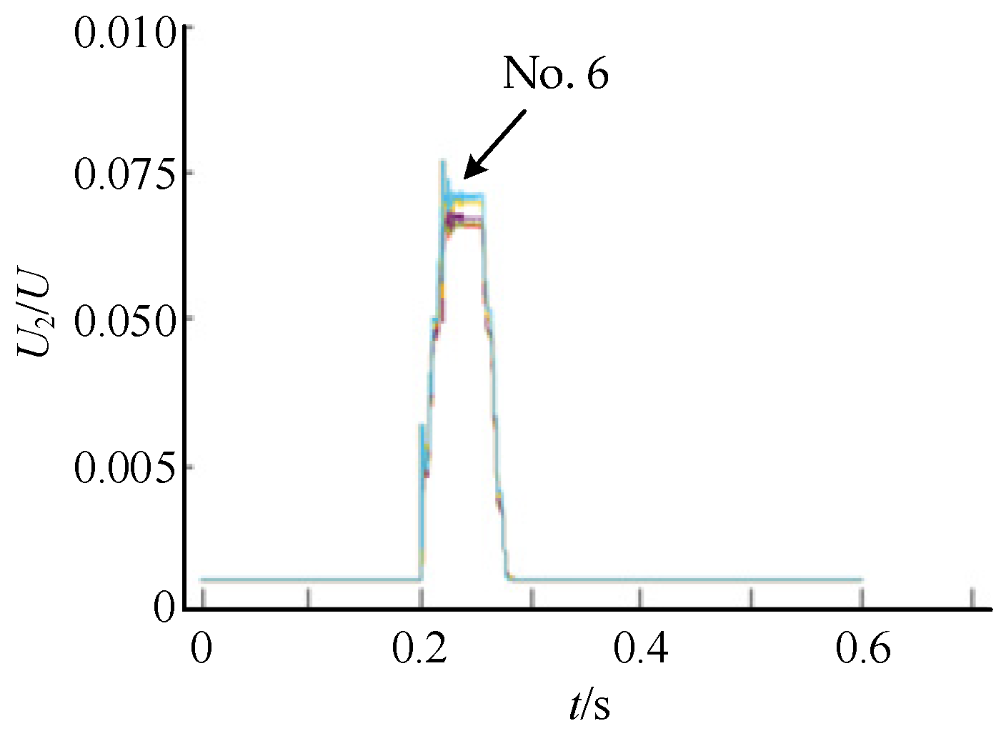
As shown in Figure 10, the faulty line is still selected as L2, with the fault occurring between transformers 6 and 7 at 0.2 s, with a ground fault resistance of 100 Ω and recovery at 0.25 s. The comparison between the ratio of negative-sequence voltage U2 to positive-sequence voltage U1 on the LV side of each transformer along line L2 is depicted in Figure 11.
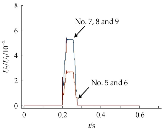
Figure 11.
Comparison of negative-sequence and positive-sequence voltage value ratios on the LV side of fault line L2 (No. 5, 6, 7, 8, and 9 transformers).
In Figure 11, the upper curve set represents the results of transformers 7, 8, and 9 downstream of the fault point, while the lower curve set represents transformers 5 and 6. After calculating the ratio coefficient η, it is evident that the ratio results on the LV side of transformers on the same side of the fault point are essentially identical, with the downstream substations showing higher values than the upstream ones. This further confirms the section of the fault point.
When the fault point is located at either end of the line, as shown in Figure 12, since all substations are on the same side of the fault point, the ratio of negative-sequence voltage U2 to positive-sequence voltage U1 is essentially the same, as depicted in Figure 13. Thus, it is not possible to determine whether the fault location is at the start or the end.
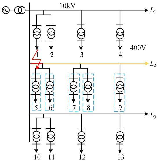
Figure 12.
Simulation system with fault points located at both ends of the line.
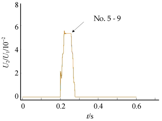
Figure 13.
Comparison of negative-sequence and positive-sequence voltage value ratios on the LV side of fault points located at both ends of the line (No. 5, 6, 7, 8, and 9 transformers).
When the fault occurs at the start of the line, as shown in Figure 14, the negative-sequence voltage value at transformer 6 at the start of the line is the highest. Therefore, it is possible to simply determine the location of the fault point at the start or end based on the magnitude of the negative-sequence voltage at each transformer.
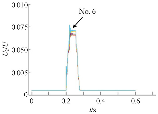
Figure 14.
Comparison of LV negative-sequence voltage values of a fault occurring at the beginning of the line (No. 5, 6, 7, 8, and 9 transformers).
Simulation analysis reveals that when a single-phase ground fault occurs on the MV side, significant variations in negative-sequence quantities can be observed on the LV side, with the magnitude of the negative-sequence quantity influenced by the fault grounding resistance.
4.2. Analysis of Dynamic Model Experimental Results
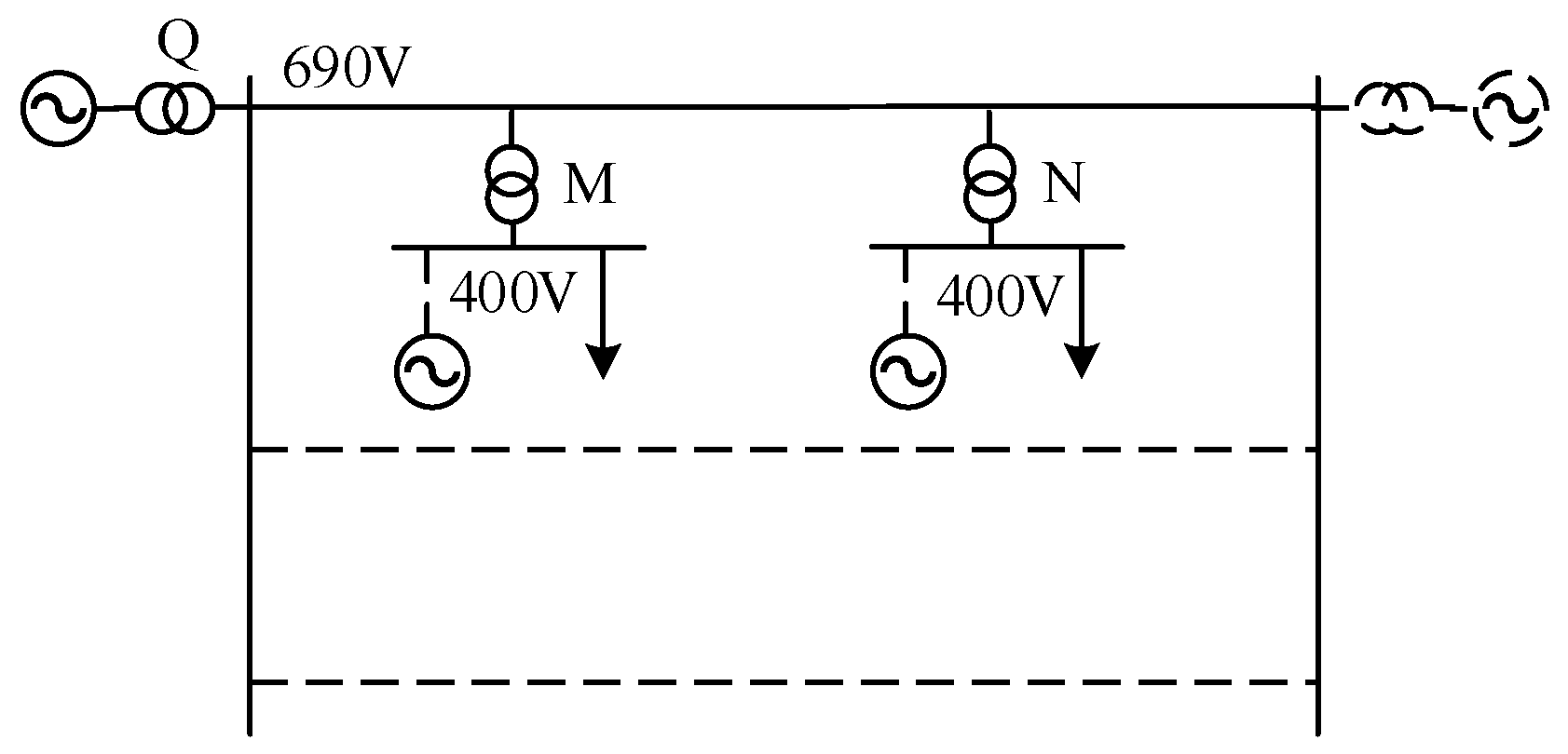
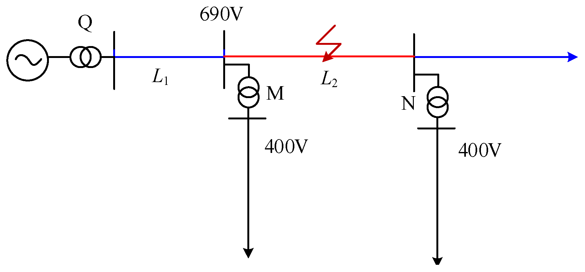
The dynamic model experiment system illustrated in Figure 15 features a simplified topology with dashed lines indicating non-operational components, as shown in Figure 16. The system comprises two voltage levels, MV 690 V and LV 400 V, with line L1 and L2 each spanning a length of 100 m. The transformer winding connections for transformers M and N are both configured as DY-type, while the main transformer Q utilizes a YD-type winding connection. The 690 V-side connection is established through a grounding transformer. Due to the limitation of the dynamic simulation topology containing only one line, the experiment focuses solely on verifying the fault characteristics on the LV side upstream and downstream of the fault point. Experimental data are sourced directly from DLP5000 recorders capturing voltage and current data from the LV side of areas M and N.

Figure 15.
Structure of dynamic simulation system.

Figure 16.
Simplified structure of dynamic simulation system (fault section L2).
4.2.1. Analysis of Fault in Section L2
When the faulted line is in section L2, the experimental conditions for tests 1 to 3 are as shown in Table 1. A single-phase grounding fault occurs in section L2 with a fault resistance of 10 Ω, and the neutral-point operation modes are as follows: ungrounded, arc suppression coil compensation, and high-resistance.

Table 1.
Experiment cases (fault section L2).
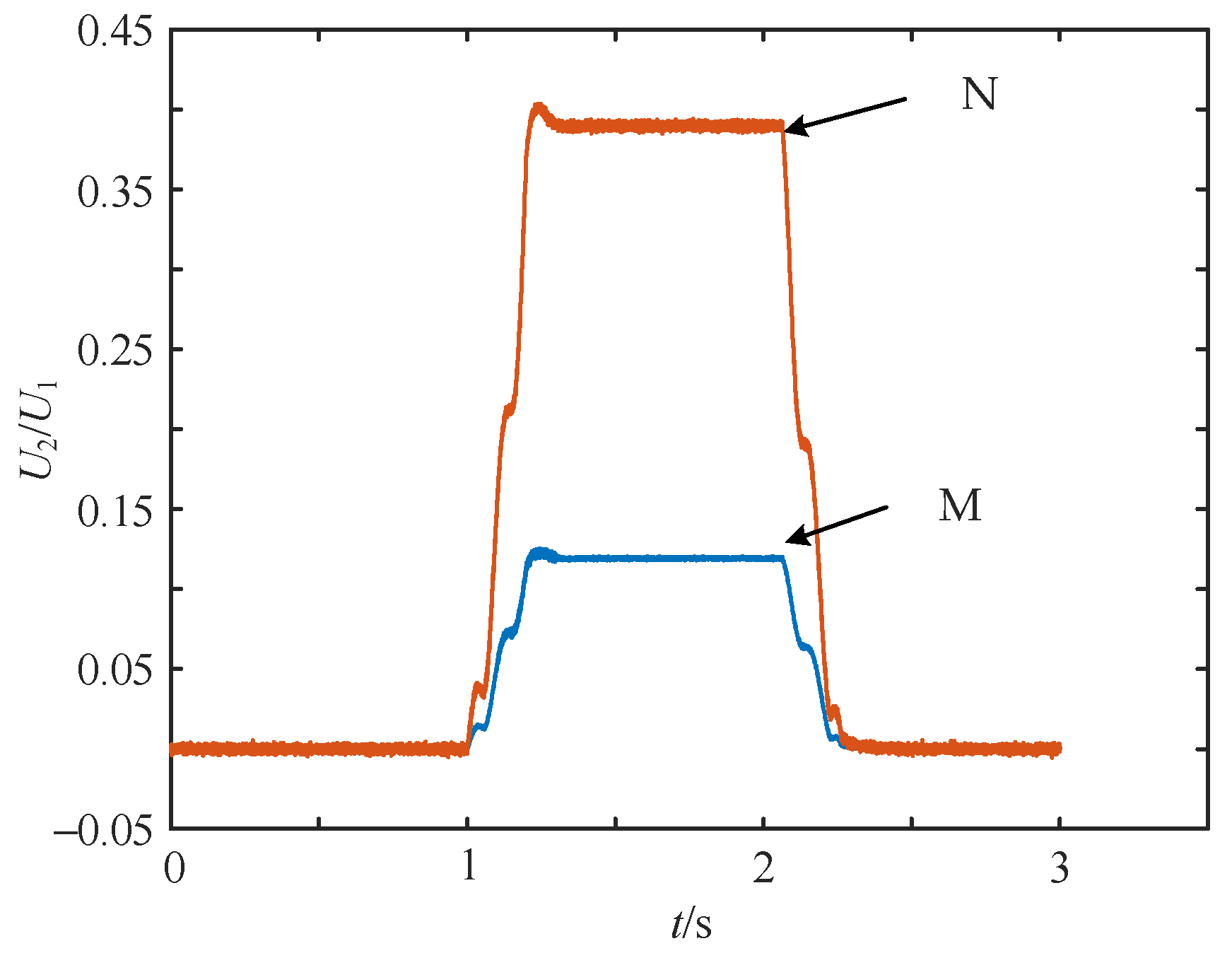
Under test condition 1, the comparison of the ratios of negative-sequence to positive-sequence voltage for transformers M and N on the LV side is shown in Figure 17.
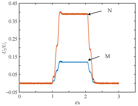
Figure 17.
Comparison of negative-sequence and positive-sequence voltage value ratios on the LV side (M and N transformers) (test condition 1).
As observed in Figure 17, following a single-phase grounding fault occurrence along section L2, the values of coefficient η on the LV side for transformers M and N on either side of the fault point exhibit significant changes. Referring to the results in Table 2, under test condition 1, the maximum value of coefficient η for transformer N downstream of the fault point reaches 0.394, surpassing the maximum value of 0.122 for the upstream transformer. This effectively identifies the position of fault section L2.
Table 2.
Experimental results of fault section L2.
As indicated in Table 2, when section L2 of the line experiences a single-phase grounding fault, under three different grounding conditions, coefficient η on the LV side of the power supply-side transformer adjacent to the fault point remains lower than that on the load side. Moreover, it is unaffected by the grounding method, aligning with theoretical expectations.
4.2.2. Analysis of Fault in Section L1
When the faulty line corresponds to the L1 section at the line’s initial end, the topological structure is depicted in Figure 18. The experimental conditions for tests 4 to 6 are outlined in Table 3, with a fault resistance of 10 Ω and neutral-point operation methods varying between ungrounded, arc suppression coil, and high-resistance.
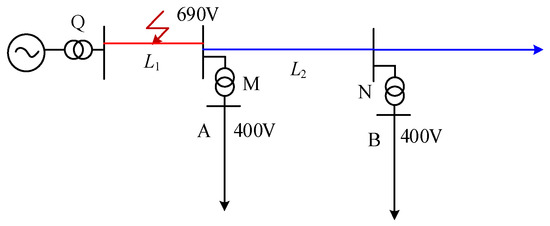
Figure 18.
Simplified structure of dynamic simulation system (fault section L1).
Table 3.
Experiment cases (fault section L1).
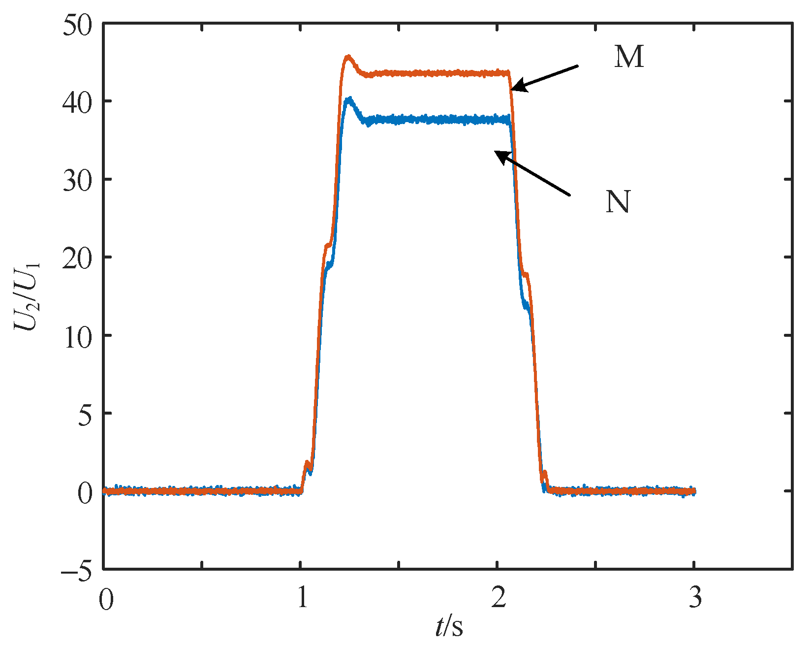
Under test condition 4, the comparison of the negative-sequence voltage on the LV side of transformers M and N is illustrated in Figure 19.
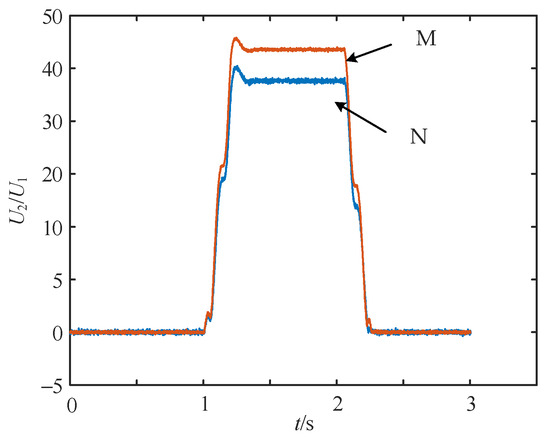
Figure 19.
Comparison of negative-sequence and positive-sequence voltage value ratios on the LV side (M and N transformers) (test condition 4).
From Figure 19, it is evident that there is a noticeable change in the negative-sequence voltage at transformers M and N on the LV side when a single-phase ground fault occurs at the beginning of line section L1. Referring to the results in Table 4, under the conditions of test 4, the maximum value of the negative-sequence voltage at transformer M, which is close to the fault point, is 46.353 V, exceeding the maximum value of 39.174 V at transformer N, which is farther downstream.
Table 4.
Experimental results of fault section L1.
According to Table 4, when the fault point is located at the beginning of the line, transformers M and N on the LV side experience simultaneous increases in negative-sequence voltage. The negative-sequence voltage at transformers near the fault point is greater than that at downstream transformers along the line, and this observation is independent of the grounding method. In summary, the results of the six experiments confirm the feasibility of the method proposed in this paper.
5. Discussion
This paper introduces a fresh perspective on tackling the issue of detecting single-phase ground faults in low-current systems. It suggests leveraging the extensive monitoring infrastructure on the LV side to utilize fault negative-sequence characteristic information for pinpointing both the faulted line and its section. This method can serve as a supplementary strategy or stand-alone diagnostic tool for identifying faults in MV systems.
In complex distribution networks, apart from the fault analysis discussed in this paper, there are many other factors to consider, such as the influence of meshed network structures and other fault factors. Additionally, the magnitude of negative-sequence voltage and current measured on the LV side is affected by fault resistance. Further refinement and analysis are needed in the future to enhance the reliability of single-phase ground fault discrimination.
This paper provides a comprehensive theoretical analysis of the negative-sequence quantity characteristics measured on the LV side. However, this technology requires further validation in field environments to meet practical operational requirements.
Author Contributions
Conceptualization, M.Z.; methodology, M.Z.; software, M.Z. and X.A.; validation, M.Z. and X.A.; formal analysis, X.A.; investigation, X.A.; resources, X.A.; data curation, M.Z.; writing—original draft preparation, M.Z.; writing—review and editing, M.Z.; supervision, X.A.; funding acquisition, X.A. All authors have read and agreed to the published version of the manuscript.
Funding
This research was supported by the National Key R&D Program of China (Grant no. 2020YFB0905900).
Data Availability Statement
The data presented in this study are available on request from the corresponding author.
Conflicts of Interest
The authors declare no conflicts of interest.
References
- Cheng, L.; Chen, Q. A survey on faulty line selection technology for single-phase grounded transmission line in small current neutral grounded system. Power Syst. Technol. 2009, 33, 219–224. [Google Scholar]
- Zhang, M.; Luan, W.; Ai, X.; Xu, B. Single-phase Grounding Fault Detection in Non-solidly Earthed Network Based on Low-voltage Measurements. Power Syst. Technol. 2023, 47, 3457–3466. [Google Scholar]
- Shao, W.; Bai, J.; Cheng, Y.; Zhang, Z.; Li, N. Research on a faulty line selection method based on the zero-sequence disturbance power of resonant grounded distribution networks. Energies 2019, 12, 846. [Google Scholar] [CrossRef]
- Li, Y.; Li, Y.; Chen, X.; Yu, J. Denoising and feature extraction algorithms using NPE combined with VMD and their applications in ship-radiated noise. Symmetry 2017, 9, 256. [Google Scholar] [CrossRef]
- Wang, S.; Sun, Y.; Zhou, Y.; Jamil Mahfoud, R.; Hou, D. A new hybrid short-term interval forecasting of PV output power based on EEMD-SE-RVM. Energies 2019, 13, 87. [Google Scholar] [CrossRef]
- Liu, F.; Gao, J.; Liu, H. The feature extraction and diagnosis of rolling bearing based on CEEMD and LDWPSO-PNN. IEEE Access 2020, 8, 19810–19819. [Google Scholar] [CrossRef]
- Liu, J.; Zhang, X.; Shen, W.; Zhang, Z. Performance testing of single phase to earth fault location for distribution network with neutral point non-effectively grounded systems. Autom. Electr. Power Syst. 2018, 42, 138–143. [Google Scholar]
- Zeng, X.; Yin, X.; Yu, Y. New methods for control and protection relay in a compensated medium voltage distribution network based on injecting various frequency current. Proc. CSEE 2000, 20, 29–32. [Google Scholar]
- Luan, X.; Wu, S.; Jia, C.; Yang, Y.; Zhang, Z.; Luo, X. Fault line selection principle of single-phase-to-ground fault based on improved zero-sequence admittance. Power Syst. Technol. 2022, 46, 353–360. [Google Scholar]
- Sang, Z.; Zhang, H.; Pan, Z.; Tian, Z. Protection for single phase to earth fault line selection for ungrounded power system by injecting signal. Autom. Electr. Power Syst. 1996, 20, 11–12+35. [Google Scholar]
- Jiang, B.; Dong, X.; Shi, S. A method of single phase to ground fault feeder selection based on single phase current traveling wave for distribution lines. Proc. CSEE 2014, 34, 6216–6227. [Google Scholar]
- Li, G.; Xue, Y.; Xu, B.; Yang, F. Analysis on arc reignition transient characteristics for grounding fault in non-solidly grounding system. Autom. Electr. Power Syst. 2020, 44, 189–196. [Google Scholar]
- Li, T.; Wang, F.; Zhu, L.; Li, J. A new method of distribution network single-phase ground fault line selection based on the intrinsic mode energy entropy. Power Syst. Technol. 2008, 32, 128–132. [Google Scholar]
- Fang, Y.; Xue, Y.; Song, H.; Guan, Y.; Yang, F.; Xu, B. Transient energy analysis and faulty feeder identification method of high impedance fault in the resonant grounding system. Proc. CSEE 2018, 38, 5636–5645. [Google Scholar]
- Xue, Y.; Xu, B.; Feng, Z.; Li, T. The principle of directional earth fault protection using zero sequence transients in non-solid earthed network. Proc. CSEE 2003, 23, 51–56. [Google Scholar]
- Xue, Y.; Feng, Z.; Xu, B.; Chen, Y.; Li, J. Earth fault protection in non-solidly earthed network based on transient zero sequence current comparison. Autom. Electr. Power Syst. 2003, 27, 48–53. [Google Scholar]
- Ye, Y.; Cai, X.; Xie, M.; Xu, B.; Wei, L. Fault phase fast detection of the single-phase-to-ground fault in a power distribution network. Power Syst. Prot. Control 2021, 49, 96–103. [Google Scholar]
- Xiao, B.; Shu, H.; Gao, F. Survey of the methods of fault line selection for single-phase-to-earth fault in networks with unground neutral. Relay 2001, 29, 16–20. [Google Scholar]
- Lv, J.; Luan, W.; Liu, R.; Wang, P.; Lin, J. Architecture of distribution internet of things based on widespread sensing & software defined technology. Power Syst. Technol. 2018, 42, 3108–3115. [Google Scholar]
- Xue, Y. Research on Single-Phase Grounding Fault Detection in Distribution Networks Based on Transient Characteristic Information. Ph.D. Thesis, Xi’an Jiaotong University, Xi’an, China, 2003. [Google Scholar]
- Zhao, M. Research on Data Perception and Intelligent Maintenance Decision of Distribution Transformers. Ph.D. Thesis, North China Electric Power University, Beijing, China, 2019. [Google Scholar]
- Zeng, X.; Yin, X.; Zhang, Z.; Chen, D. Study for negative sequence current distributing and ground fault protection in middle voltage power systems. Proc. CSEE 2001, 21, 84–89. [Google Scholar]
- Xu, B.; Li, T.; Xue, Y. Distribution Network Relay Protection and Automation; China Electric Power Press: Beijing, China, 2017; pp. 120–125. [Google Scholar]
- He, J.; Li, Y.; Dong, X.; Li, B. Relay Protection of Power System, 4th ed.; China Electric Power Press: Beijing, China, 2010; pp. 72–90. [Google Scholar]


Disclaimer/Publisher’s Note: The statements, opinions and data contained in all publications are solely those of the individual author(s) and contributor(s) and not of MDPI and/or the editor(s). MDPI and/or the editor(s) disclaim responsibility for any injury to people or property resulting from any ideas, methods, instructions or products referred to in the content. |
© 2024 by the authors. Licensee MDPI, Basel, Switzerland. This article is an open access article distributed under the terms and conditions of the Creative Commons Attribution (CC BY) license (https://creativecommons.org/licenses/by/4.0/).