Early Fault Diagnosis of Bearings Based on Symplectic Geometry Mode Decomposition Guided by Optimal Weight Spectrum Index

Abstract

When the rotating machinery fails, the signal generated by the faulty component often no longer maintains the original symmetry, which makes the vibration signal with nonlinear and non-stationary characteristics, and is easily affected by background noise and other equipment excitation sources. In the early stage of fault occurrence, the fault signal is weak and difficult to extract. Traditional fault diagnosis methods are not able to easily diagnose fault information. To address this issue, this paper proposes an early fault diagnosis method for symplectic geometry mode decomposition (SGMD) based on the optimal weight spectrum index (OWSI). Firstly, using normal and fault signals, the optimal weight spectrum is derived through convex optimization. Secondly, SGMD is used to decompose the fault signal, obtaining a series of symplectic geometric modal components (SGCs) and calculating the optimal weight index of each component signal. Finally, using the principle of maximizing the OWSI, sensitive components reflecting fault characteristics are selected, and the signal is reconstructed based on this index. Then, envelope analysis is performed on the sensitive components to extract early fault characteristics of rolling bearings. OWSI can effectively distinguish the interference components in fault signals using normal signals, while SGMD has the characteristic of unchanged phase space structure, which can effectively ensure the integrity of internal features in data. Using actual fault data of rolling bearings for verification, the results show that the proposed method can effectively extract sensitive components that reflect fault characteristics. Compared with existing methods such as Variational Mode Decomposition (VMD), Feature Mode Decomposition (FMD), and Spectral Kurtosis (SK), this method has better performance.

1. Introduction

Rolling bearings are one of the most important key components of rotating machinery and are often used in rail transit, aerospace and petrochemical industries [1,2]. Due to the harsh working environment, they often face high speed, high pressure and other conditions, and often fail. Especially when early failure occurs, the fault signal is susceptible to the impact of background noise and other equipment incentive sources; if not found in time, this may easily lead to production suspension and economic losses, and in serious cases, even endanger the safety of human life [3,4]. Therefore, both the condition detection and fault diagnosis of rolling bearings are very important for the safe operation of mechanical equipment.

Rolling bearings are composed of four parts: inner ring, outer ring, rolling element and cage. When a bearing component fails, the destruction of signal symmetry may be caused by a variety of factors. For example, faults such as rotor imbalance, misalignment, looseness or rub impact may lead to asymmetric signal waveform, and corresponding fault characteristic frequency will appear in the frequency domain [5]. The fault characteristics can be extracted by testing the vibration signal of the bearing. However, when the bearing experiences early failure, the fault characteristic frequency is often submerged in the noise interference, which makes it difficult to effectively extract the sensitive components related to the fault and affects the fault identification.

Therefore, scholars have designed many noise reduction problems for bearing fault diagnosis. Among these commonly used fault signal processing techniques, time-frequency analysis (TFA), empirical mode decomposition (EMD), wavelet transform (WT), and singular value decomposition (SVD) are the most prominent, and these methods help to identify the fault characteristics of bearings. Time-frequency analysis is a good method to capture the characteristics of time-varying non-stationary signals, which has been proven to be effective for the analysis of bearing vibration signals under actual operating conditions [6,7,8]. Yu [9] proposed a transient-extraction transform (TET) for instantaneous pulse signals, which was successfully applied to the characterization of the transient characteristics of bearing fault signals. Miao [10] proposed an automatic instantaneous frequency estimation method, which can realize instantaneous frequency estimation and feature extraction of a variable number of multi-component signals. Wang et al. [11] proposed a data-driven adaptive chirp mode decomposition (DD-ACMD) method. By introducing an instantaneous frequency estimation method based on signal derivative normalization, the adaptability of the ACMD method to multi-component signals and noise robustness are improved, and the method has been successfully applied to fault diagnosis of rolling bearings and the axle box of a heavy locomotive under variable speed conditions. Zhang et al. [12] used time-frequency images as the input of enhanced convolutional neural networks to achieve accurate identification of bearing fault types. The method of time-frequency analysis can solve the problem of fault feature extraction and identification in time-varying working conditions, but for early faults, limited by noise interference, it is easy to cause energy divergence, and fault features are easily submerged in the background noise.

As a data-driven adaptive decomposition method, EMD can decompose complex signals into several eigenmode functions, so as to identify bearing fault information. Notable advancements include Xia et al.’s [13] implementation of a double iterative EMD to mitigate the effects of local polar deviation, Lashari et al.’s [14] application of a time-varying filtered EMD for single-channel system identification, and Wu et al.’s [15] introduction of an improved version of EMD, termed Ensemble Empirical Mode Decomposition (EEMD), to enhance fault detection in rotating machinery. Furthermore, Lei et al. [16] and Li et al. [17] have refined EEMD through improved adaptive resonance techniques, demonstrating their effectiveness in the fault diagnosis of bearings. Despite their utility, these algorithms, reliant on iterative time-domain calculations, suffer from low computational efficiency and are vulnerable to cumulative errors, significantly impacting the precision of the final modal decomposition.

As a typical noise reduction method, wavelet transform (WT) can deeply mine local information of data and extract weak fault features hidden in local areas [18,19,20,21]. The signal is decomposed into a series of wavelet coefficients, which represent the characteristics of the signal at different scales and different positions, through the stretching and shifting wavelet basis function. Through multi-scale analysis, the detailed information and low-frequency components in the signal can be separated, so as to realize the noise reduction and feature extraction of the signal. In fault diagnosis, wavelet decomposition can effectively remove the noise in the signal and improve the signal-to-noise ratio of the fault signal by means of threshold processing. However, wavelet transform has the following fatal shortcomings [22]: (1) As a Fourier transform with adjustable window size, wavelet transform has the problem of modal confusion. (2) When the signal is decomposed by wavelet transform, the wavelet basis needs to be selected according to prior knowledge. The decomposition of the same signal by different wavelet bases will produce different results, so the wavelet transform is not self-adaptive. (3) When the noise is low, the noise reduction effect of wavelet transform is not ideal.

The field of signal denoising via matrix decomposition has increasingly captivated scholarly interest. Singular Value Decomposition (SVD) stands out as a notable technique in this realm. Sun et al. [23] utilized an enhanced SVD approach to mitigate the ambiguities associated with the original SVD’s reconstruction order and its limited noise reduction capability, facilitating the extraction of the bearing’s fault characteristic frequency. Zhang et al. [24] introduced a time-variant SVD technique to accentuate periodic faults and successfully extract the fault eigenfrequencies of bearings. Yang et al. [25] used amplitude filtering and the negative entropy index as screening indexes to extract effective singular values and retain effective fault information after reconstruction. Although SVD effectively reduces noise by matrix decomposition and discarding eigenvectors associated with small eigenvalues, in the case of strong background noise, the effect is often poor, resulting in incomplete noise reduction and retaining some interference components.

In recent years, relevant researchers have abandoned traditional research ideas and proposed constraint optimization methods to complete signal decomposition [26]. For example, Dragomiretskiy et al. [27] proposed a variational mode decomposition (VMD) method to transform the signal decomposition into a constrained variational problem, thus adaptive decomposition into multiple eigenmodal components. However, in the VMD method, the number of decomposition modes needs to be predetermined [28]. Li et al. [29] improved the adaptive aspects of VMD and sparse coding. Although the sparse coding algorithm has a good denoising ability, its denoising threshold cannot be manually drafted, and the purpose of adaptive denoising cannot be realized. Moreover, the Minimum Entropy Deconvolution (MED) method was innovated to negate the effects of the transmission path, premised on the notion of an impulsive original excitation to maximize kurtosis through the identification of an inverse filter [30]. Endo et al. [31] were pioneers in applying MED for fault detection, achieving promising outcomes. McDonald et al. [32] critiqued MED for its propensity to deconvolve isolated or select pulses rather than the anticipatory periodic pulses seen during fault cycles, thereby proposing the Maximum Correlated Kurtosis Deconvolution (MCKD) as a method geared towards deconvolving periodic pulse faults by acknowledging the fault’s periodic nature. Recently, MCKD has been widely adopted for extracting periodic pulse signals in fault diagnosis [33]. Miao et al. [34] introduced the Feature Mode Decomposition (FMD) algorithm, proving its superiority over VMD in fault signal decomposition. FMD draws upon blind deconvolution theory, integrating it into the signal decomposition process to bolster the filtering of complex signals with indeterminate transfer functions and unpredictable noise [35].

The Symplectic Geometric Similar Transform (SGST) method represents a matrix decomposition-based signal processing technique [36], achieving adaptive signal transformation while preserving the integrity of the original signal structure. SGST’s enhanced classification performance has spurred the development of improved algorithms, such as the Adaptive Weighted Sim-geometric Decomposition (AWSGD) method proposed by Cheng et al. [37], which leverages period kurtosis for adaptive signal decomposition. Zhang et al. [38] introduced an advanced Symplectic Geometric Modal Decomposition (SGMD) technique, proposing a novel fault diagnosis approach based on the refined Sim-geometric modal decomposition, although its applicability to noise-dominated signals remains limited. Hou et al. [39,40] proposed the concept of an optimal weight spectrum, extracting fault components based on the optimal weight spectrum index within VMD and WT methodologies, showcasing effective performance. Nevertheless, the efficacy of the optimal weight spectral index in the context of matrix transformation denoising remains an area ripe for exploration.

To solve the problems discussed above, this paper proposes a fault diagnosis method for SGMD based on the optimal weight spectrum index. The contributions of this work are as follows:

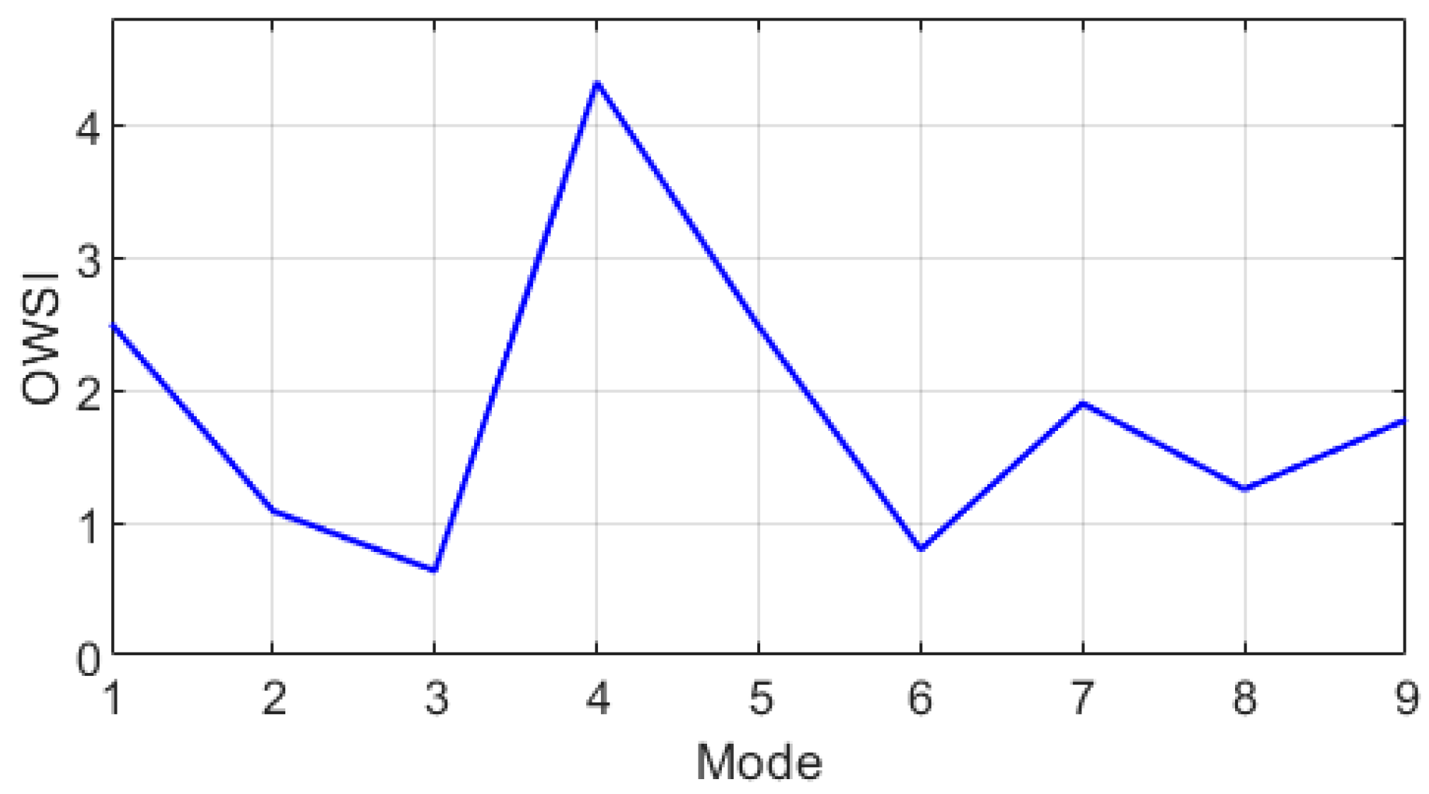
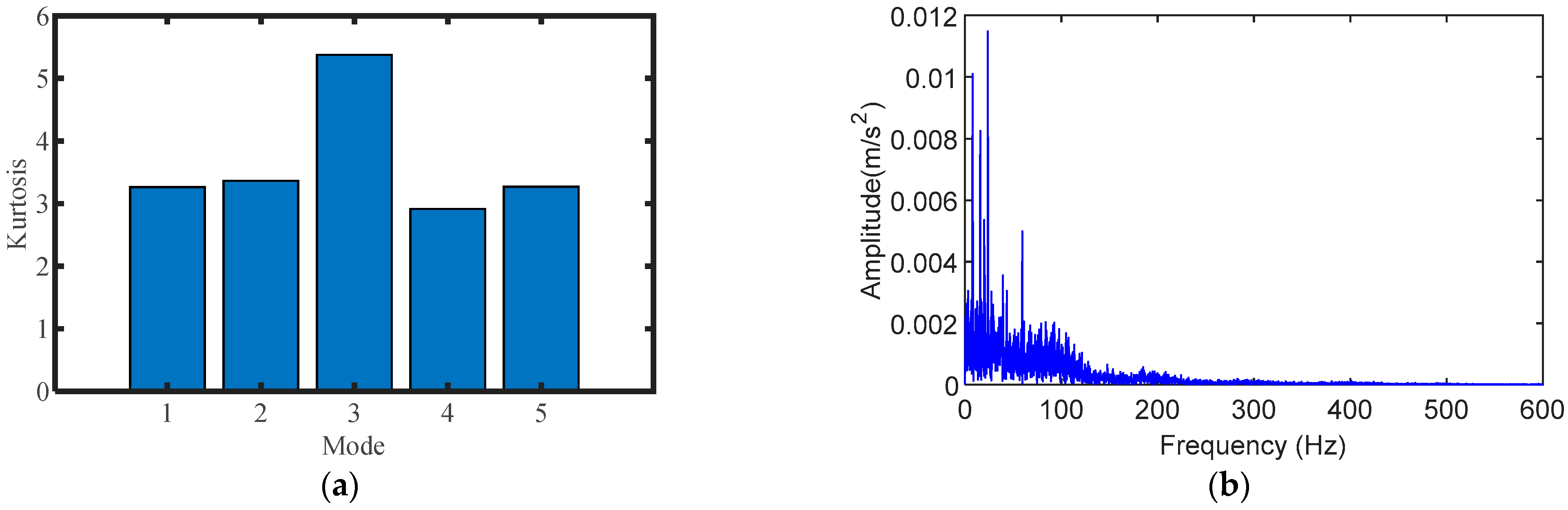
• An SGMD signal reconstruction method guided by the optimal weight spectrum index is proposed to screen out sensitive components reflecting fault characteristics and reduce the influence of noise and interference components.
• Using the information of health and fault signals, the optimal weight spectrum is generated to generate effective fault indicators and provide a robust framework for fault detection.
• Validation of the proposed methodology can be conducted through signal experiments focused on early bearing faults, which substantiates its efficacy in practical applications.

The remaining sections of this paper are arranged as follows: Section 2 is the theoretical introduction of SGMD Guided by Optimal Weight Spectrum Index, which lays the foundation for the method proposed in this paper. Section 3 is the entire process of the method proposed, offering a step-by-step guide to its implementation. Section 4 presents an analysis of experimental signals, demonstrating the method’s applicability and effectiveness in real-world scenarios. Finally, Section 5 provides a summary, encapsulating the key findings and contributions of this study.

2. Methodological Theory

2.1. Optimal Weight Spectrum Theory

Hou et al. [37] introduced a concept of optimal weight spectrum using convex optimization technology to identify fault and interference components in signals, which showed good performance in practical applications. Below is an introduction to the theory. Suppose a set of signals is represented by $x=[x_1,x_2,\dots ,x_n]$, where n is the number of sampling points. The Fourier spectrum of the signal x is defined as $FS=fft(x)$ , where $fft(\cdot )$ represents the fast Fourier transform, and the normalized Fourier spectrum is defined as follows:

$$NFS=FS/{\Vert FS\Vert }_{L1}$$

(1)

In real industry, most of the data obtained are normal data. The main difference between the fault signal and the normal signal is that there are some narrowband fault components in the fault data, while there are interference components and noise related to machinery and equipment in most health data. These interference components also exist in the fault signals tested by the same equipment. The useful information in these health signals can be used to denoise the fault signals and screen out the sensitive components that reflect the fault characteristics. Suppose that $P$ and $Q$ samples of normal signal and fault signal are collected and the corresponding sample sets are denoted as ${\left\{x_H\right\}}^P$ and ${\left\{x_F\right\}}^Q$, respectively. Furthermore, the normalized Fourier spectrum set of the healthy and faulty signal sets can be calculated, which can be expressed as ${\left\{NF{S}_H\right\}}^P$ and ${\left\{NF{S}_F\right\}}^Q$. Based on the aforementioned two sets, OWS can be obtained in the following ways. First, a sum of weighted normalized Fourier spectrum ($SWNFS$) [38] is defined as follows:

$$SWNFS={\omega }^{T}NFS+b=0$$

(2)

where $\omega$ is a weights vector, and $b$ is a bias. The $SWNFS$ can be conceptualized as a hyperplane in a high-dimensional space, where ${\left\{NF{S}_H\right\}}^P$ and ${\left\{NF{S}_F\right\}}^Q$ represent two point clusters. The primary purpose of the hyperplane is to optimize the separation between the two point clusters. By utilizing maximum logarithmic likelihood estimation, an objective function to achieve the maximum distance is defined as follows:

$$\begin{array}{cc}\hfill \min L(\xi )& =\frac{1}{2(P+Q)}\lambda {\xi }^T\xi \hfill \\ & +\frac{1}{2(P+Q)}{\displaystyle \sum _{i=1}^{P+Q}\left[-y_i{\xi }^T{\rho }_i+\log (1+\exp ({\xi }^T{\rho }_i))\right]}\hfill \end{array}$$

(3)

where $\xi ={\left[{\omega }^{T}b\right]}^T$, ${\rho }_i={\left[{(NF{S}^i)}^{T}1\right]}^T$; $\lambda$ is the coefficient of the regularization item, $y_i$ is label variable, if $NF{S}^i\in {\left\{NF{S}_H\right\}}^P$, $y_i=0$; if $NF{S}^i\in {\left\{NF{S}_F\right\}}^Q$, $y_i=1$. The objective function in Equation (3) can be easily solved by using the gradient descent method, and the obtained optimal weights ${\omega }^{\ast }$ is named optimized weights spectrum ($OWS$) [39].

Based on OWS, the optimal weight spectrum index ($OWSI$) is defined as follows:

$$OWSI(SCG)={\left({\omega }^{*}\right)}^{T}F{S}_{SGC},whereF{S}_{SGC}=\left|fft(SGC)\right|$$

(4)

where $SGC$ is the component decomposed by SGMD, and the specific form is explained in Section 2.2. Reference for specific properties of $OWSI$ can be found in [40].

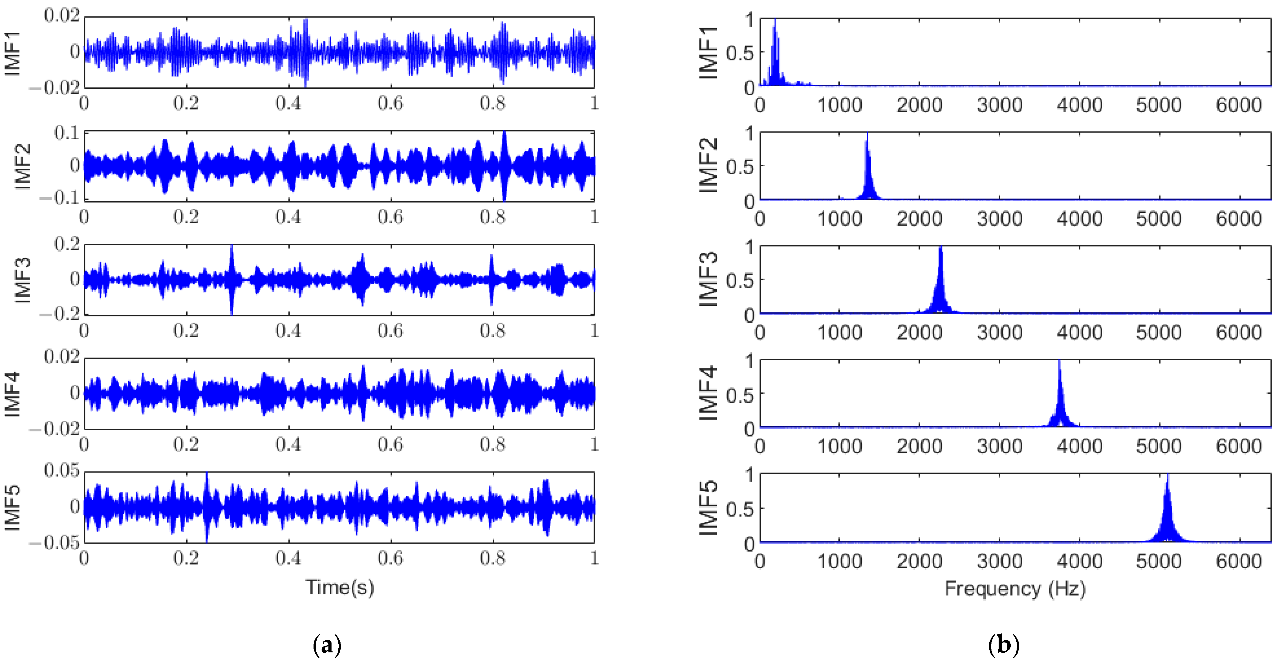
2.2. The Theory of SGMD

SGMD is a new mode decomposition method which applies the symplectic geometric QR decomposition method to the Hamilton matrix, obtains corresponding eigenvalues and eigenvectors, and finally reconstructs the SGCs by diagonal averaging [38]. The advantage of symplectic transformation is that it can keep the phase space of the data structure unchanged and ensure the integrity of the decomposed signal. Suppose a one-dimension time-series vibration signal $x=[x_1,x_2,\dots ,x_n]$, where n represents the length of the data, and using the Takens embedding theorem, construct the trajectory matrix $X$, expressed as follows:

$$X=\left[\begin{array}{cccc}{x}_1& x_{1+\tau }& \dots & x_{1+(d-1)\tau }\\ x_2& x_{2+\tau }& \dots & x_{2+(d-1)\tau }\\ ⋮& ⋮& \ddots & ⋮\\ x_m& x_{m+\tau }& \dots & x_{m+(d-1)\tau }\end{array}\right]$$

(5)

where d represents the embedding dimension, $\tau$ represents the delay time and has $m=n-{(d-1)}^{\tau }$, according to reference [33]; the PSD of the original signal $x$ is calculated and the frequency fmax at the maximum peak is found, and the other frequency fmax is compared with the sampling frequency fs, when the ratio is less than the set threshold, $d=n/3$. Otherwise, $d=1.2\times (fs/f\max )$, $\tau =1$.

Autocorrelation analysis was performed on $X$ to obtain the covariance matrix $A$.

$$A=X^{\mathrm{T}}X$$

(6)

The equation between the Hamilton matrix $M$ is established using the covariance matrix $A$ as follows:

$$M=\left[\begin{array}{cc}A& 0\\ 0& -A^{\mathrm{T}}\end{array}\right]$$

(7)

Then, construct the Sin-geometry matrix G according to Equation (3), which can be expressed as follows:

$$Q^{\mathrm{T}}GQ=\left[\begin{array}{cc}B& R\\ 0& -B^{\mathrm{T}}\end{array}\right]$$

(8)

where $G=M^2$, the matrices $Q$ and $B$ are the sinusoidal and upper triangular matrices, respectively.

Calculate the eigenvalue ${\lambda }_1,{\lambda }_2,\dots ,{\lambda }_d$ of the upper triangular matrix $B$, which can be obtained from the properties of the Hamilton matrix, and the eigenvalue of matrix $A$ is ${\sigma }_i=\sqrt{{\lambda }_i}(i=1,2,\dots ,d)$, $Q_i(i=1,2,\dots ,d)$ is the eigenvector of matrix $A$ corresponding to the eigenvalue ${\sigma }_i$. The symplectic geometric spectrum will be arranged according to the characteristic values from the largest to the smallest, and the smaller the characteristic value, the less the characteristic information it contains and the greater the noise.

Decomposition of the matrix $A$ using $QR$ decomposition leads to the eigenvector matrix $Q$. The coefficient matrix S is constructed using the eigenvector matrix $Q$ and the original trajectory matrix $X$.

$$S_i=Q_i^{\mathrm{T}}X$$

(9)

Furthermore, the reconstruction matrix $Z$ is obtained using the eigenvector matrix $Q$ and the coefficient matrix $S$:

$$Z_i=Q_i{S}_i$$

(10)

where $Z_i(i=1,2,\dots ,d)$ is the initial single component reconstruction matrix. At this point, the original phase space reconstruction matrix $Z$ consisting of $d$ sets of reconstruction matrices can be written as $Z=Z_1+Z_2\dots +Z_d$.

The $Z_i$ obtained by single geometric similarity transformation is an $m\times d$ reconstruction matrix. Since the reconstructed single component matrix is a non-one-dimensional vibration signal, it is necessary to convert the single component matrix $Z_k(1\le k\le d)$ into a vibration signal of length $n$. The diagonal averaging method, as a common conversion algorithm, has the ability of accurate information conversion. Therefore, in this section, the single component reconstruction matrix $Z_i$ is transformed into a one-dimensional single component time series of length n by using the diagonal average method. Thus, a single component signal with d group length is obtained, and the sum of these single component signals is the original signal. Suppose the element in $Z_i$ is $z_{ij}(1\le i\le m,1\le j\le d)$. Set $d^{*}=\min (m,d)$, $m^{*}=\max (m,d)$ and $1\le i\le m,1\le j\le d$, if $m<d$, then there is $z_{ij}^{*}=z_{ij}$, otherwise $z_{ij}^{*}=z_{ji}$; according to the literature [23], the expression of the diagonal averaging transformation is as follows:

$$y_k=\{\begin{array}{c}\frac{1}{k}{\displaystyle \sum _{p=1}^k{z}_{p,k-p+1}^{*}1\le k\le d^{*}}\\ \frac{1}{d^{*}}{\displaystyle \sum _{p=1}^{d^{*}}{z}_{p,k-p+1}^{*}{d}^{*}\le k\le m^{*}}\\ \frac{1}{n-k+1}{\displaystyle \sum _{p=k-m^{*}+1}^{n-m^{*}+1}{z}_{p,k-p+1}^{*}{m}^{*}<k\le n}\end{array}$$

(11)

Equation (11) enables the conversion of the initial single-component reconstruction matrix $Z_i$ into a one-dimensional time-series $Y_i$. The diagonal averaging of each initial single-component reconstruction matrix results in a one-dimensional time-series, which further yields d sets of initial single-component signals, denoted as $Y_1,Y_2,\dots ,Y_{\mathrm{d}}$.

The single-component signals obtained by constructing trajectory matrix and matrix decomposition are not independent, and the components may have the same periodic and frequency components. Therefore, it is necessary to reconstruct each initial single component. In this paper, periodic similarity is used as the evaluation index, and component recombination is carried out for the obtained components. The matrix $Y$ is a $d\times n$ matrix. Since the main components are distributed in the front of the matrix, the periodic similarity between $Y_1$ and the other components is compared. The component with higher similarity is reconstructed and the first component SGC₁ is obtained. The components participating in SGC₁ reconstruction are removed from the matrix $Y$, the matrix of the remaining components can be represented as ${\mathrm{R}}^1$, and the sum of the matrices gives the residual signal $r^i$. The normalized mean square error ($\mathrm{NMSE}$) between the original signal and the remaining signal can be expressed as follows:

$${\mathrm{NMSE}}^h=\frac{{\displaystyle \sum _{i=1}^n}{r}^h(i)}{{\displaystyle \sum _{i=1}^n}x(i)}$$

(12)

where $h$ is the number of iterative decomposition times. The decomposition process terminates when the $\mathrm{NMSE}$ falls below the specified threshold. If it exceeds the threshold, we employ the residual term matrix as the iterative original matrix and repeat the aforementioned iteration process until meeting the termination condition. The resulting outcome of decomposition after optimization is presented as follows:

$$x(n)=\sum _{h=1}^{\mathrm{T}}SG{C}^h(n)+r^{(\mathrm{T}+1)}(n)$$

(13)

where T is the number of decomposition components obtained.

3. The Process of the Proposed Method

To mitigate the impact of noise on the diagnosis of fault signals, this study employs the Optimal Weight Spectrum Index (OWSI) to quantify the characteristics of both fault and interference components. It strategically selects components that are indicative of fault characteristics from the Symplectic Geometric Modal Decomposition (SGMD) output. The methodology proposed in this article is elucidated through a systematic process, graphically represented in Figure 1, and encompasses four distinct steps:

Step 1: Decomposition of the Fault Signal: The initial step involves applying SGMD to the fault signal under analysis. This decomposition yields a series of Symplectic Geometry Components (SGCs), effectively segregating the fault signal into its constituent modal components.

Step 2: Generation of the Optimal Weight Spectrum: Subsequently, the optimal weight spectrum is generated by leveraging both normal and fault signals. This process involves analyzing these signals to derive an optimal weight spectrum index, which serves as a quantitative measure for distinguishing between healthy and faulty signal characteristics.

Step 3: Calculation and Application of the Optimal Weight Spectral Index: For each SGC obtained from the decomposition, the optimal weight spectral index is calculated. This index is then used to guide the reconstruction of the signal, focusing on those components that are most reflective of fault characteristics based on their weighted significance.

This structured approach aims to enhance the precision and reliability of fault signal diagnosis by effectively reducing noise interference and emphasizing the signal components most relevant to fault detection.

4. Experimental Verification and Discussion

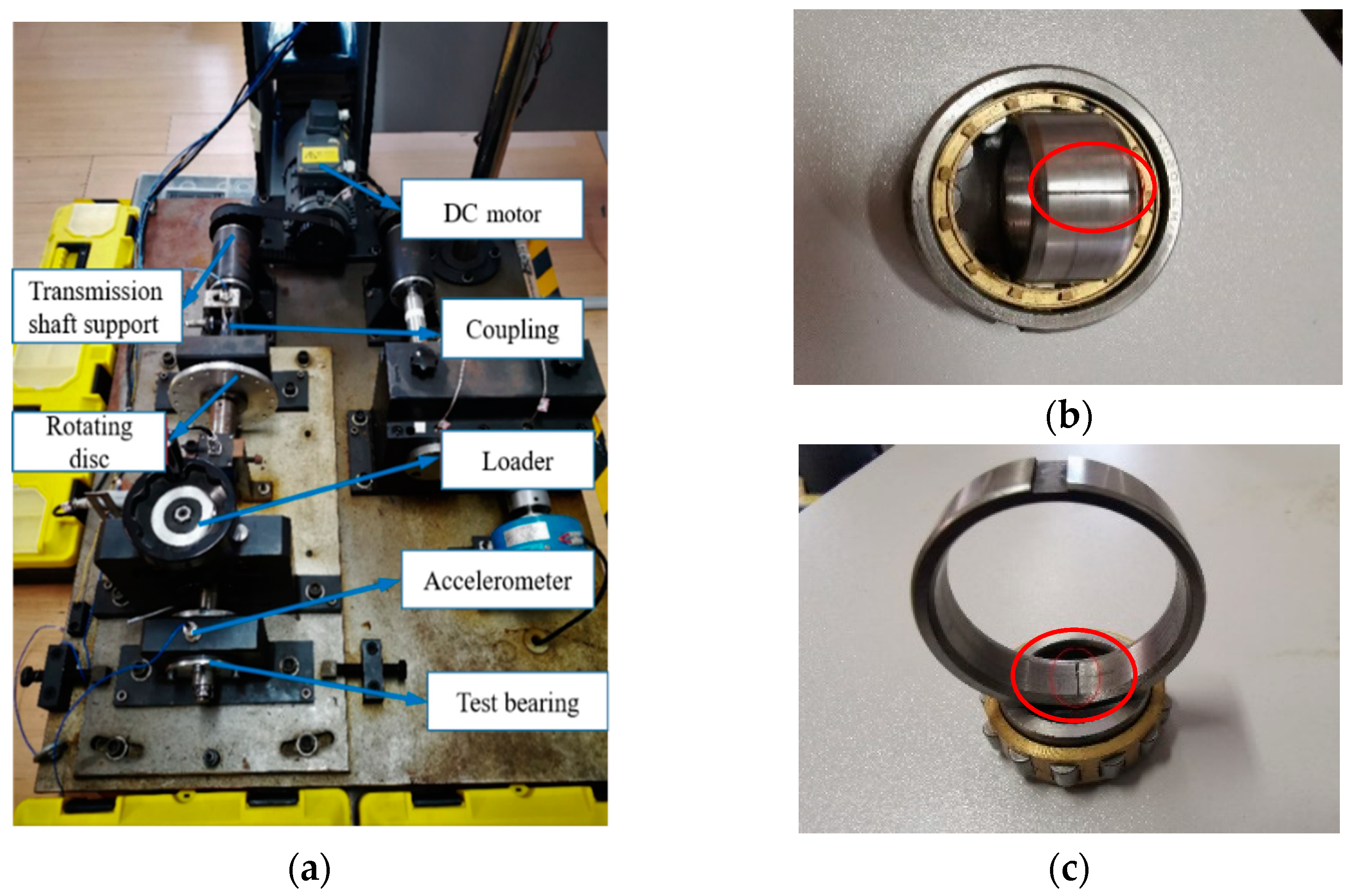
4.1. Experimental Setup

To validate the efficacy of the proposed methodology, an experimental test bench was constructed, as depicted in Figure 2a. This bench comprises several key components essential for simulating bearing faults: a DC motor, transmission shaft support, coupling, rotating disc, loader, and test bearings. These test bearings are designed to be interchangeable, allowing for the simulation of various fault conditions, including inner and outer ring faults, as illustrated in Figure 2b,c. The faults within the bearings were meticulously introduced through precision wire cutting to replicate real-world bearing failure scenarios accurately. The fault width and depth of the inner and outer rings are both 1 mm. Fault length is 4 mm.

The bearing model utilized in this study is the NU205EM/PS, with specific parameters listed in

Table 1. Bearing dimension table.

Bearing Type	NU205EM/PS
Inner race diameter (mm)	25
Outer race diameter (mm)	52
Rolling element diameter (mm)	7.5
Pitch diameter (mm)	39
Roller number	13
Contact angle α (°)	0

. The experimental setup was configured with a sampling frequency of 12,800 Hz, a sampling duration of 1 s, and a rotational speed of 1200 revolutions per minute (r/min), to ensure that the collected data accurately reflect the dynamics of bearing operation under fault conditions. Figure 3a,b show the data obtained from the test bench, showing the health data and fault data of the bearing vibration signal, respectively. Data collection using LabVIEW edited the collection program.

With the operating parameters of the bearing firmly established, this study proceeds to calculate the characteristic failure frequencies of the bearing’s inner ring. These calculations are critical for identifying the specific frequencies associated with different types of bearing faults and are detailed in

Table 2. The bearing failure characteristic frequency formula.

Failure Name	Fault Characteristic Frequency Calculation Formula	Failure Frequency
inner ring failure	$f_i=\frac{r}{120}n\left(1+\frac{d}{D}\cos \alpha \right)$	155 Hz
outer ring failure	$f_o=\frac{r}{120}n\left(1+\frac{d}{D}\cos \alpha \right)$	105 Hz

. This comprehensive approach, combining a practical test bench setup with detailed analytical calculations, aims to rigorously evaluate the performance and reliability of the proposed fault diagnosis method under controlled, yet realistic, conditions.

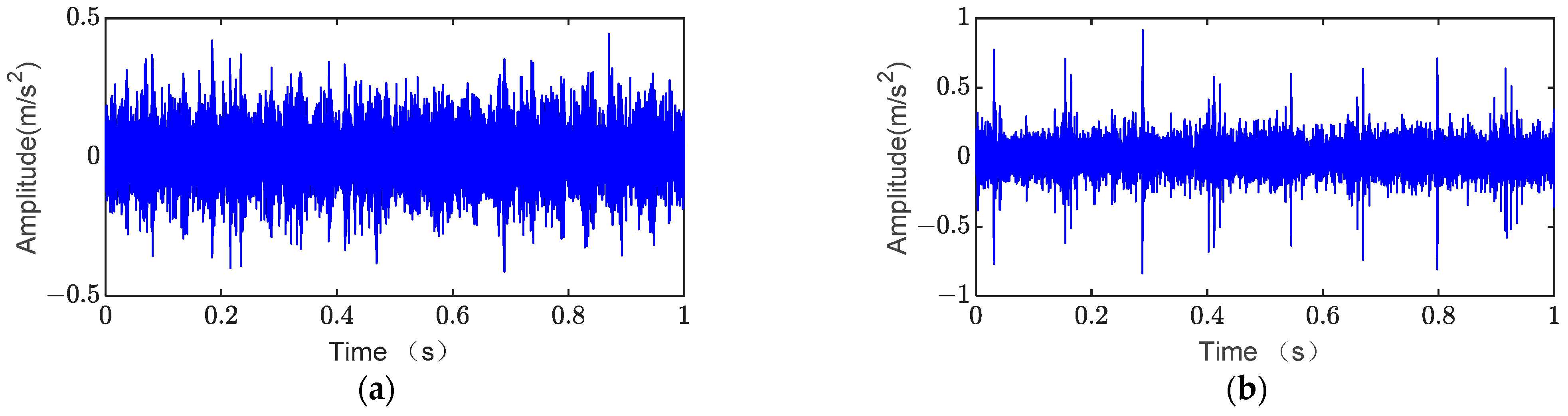
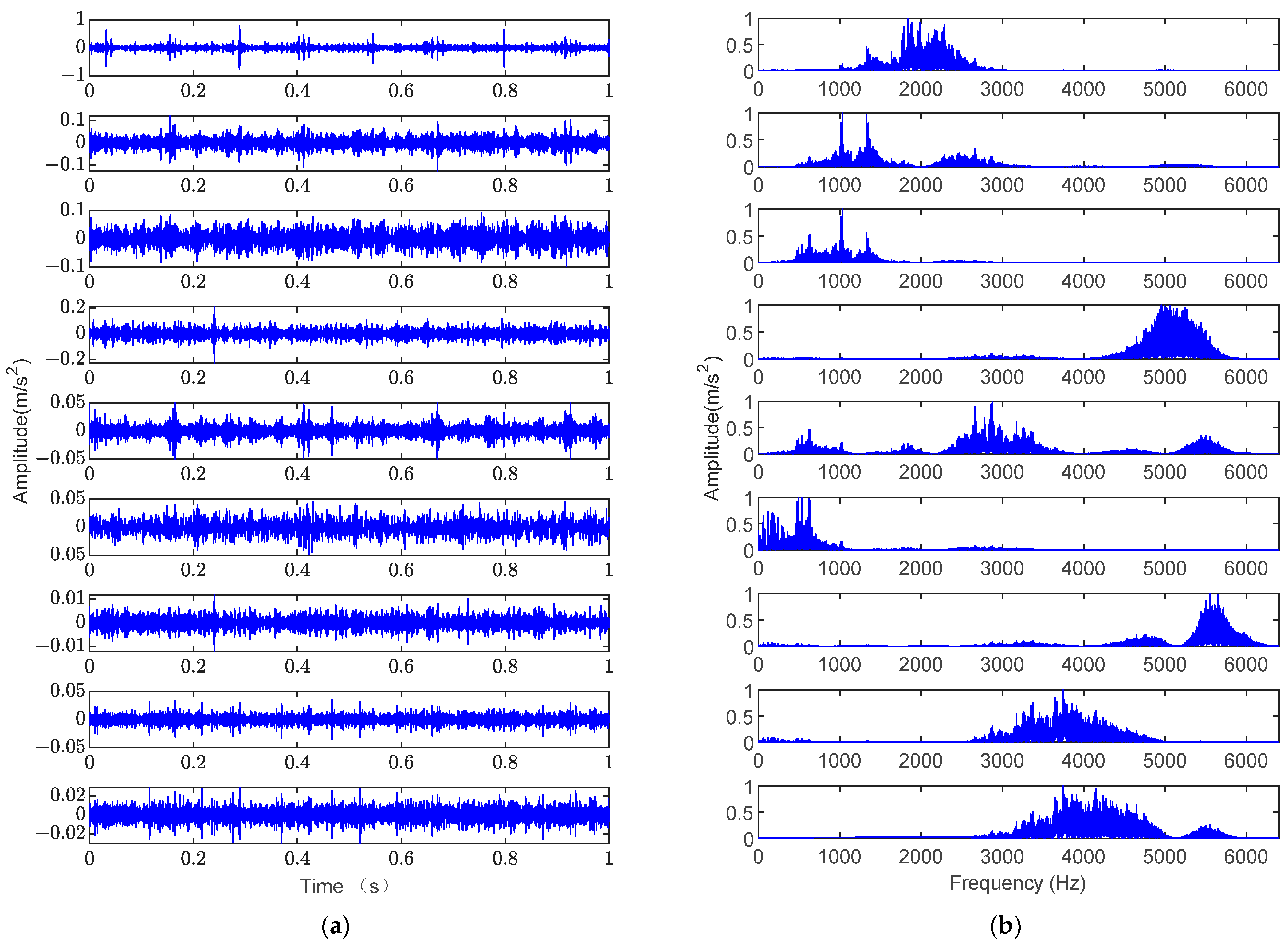
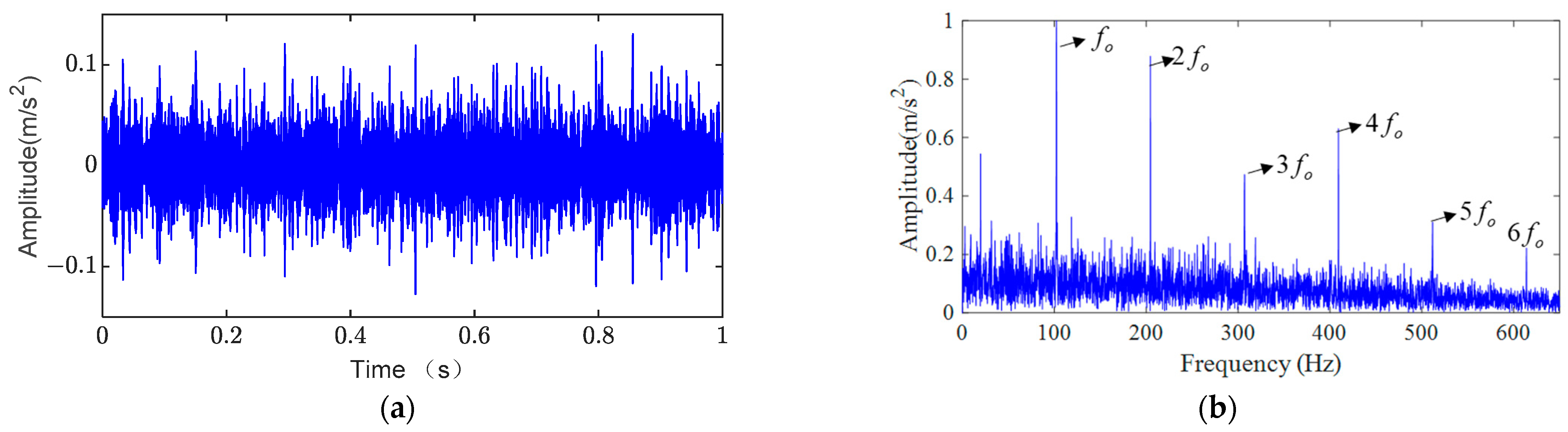
4.2. Outer Ring Fault Analysis

Firstly, at a constant speed of 1200 rpm, collect signals from some normal bearings and some faulty outer ring bearings. The time-domain diagram is shown in Figure 3. Then, collect the signal of the outer ring faulty bearing and use the method proposed in this article for analysis.

The process of verifying the proposed method’s effectiveness involved generating an optimal weight spectrum from collected normal and fault signals, as illustrated in Figure 4. Subsequently, the signal under scrutiny was decomposed using Symplectic Geometric Modal Decomposition (SGMD), with the decomposition parameters set based on empirical values. The outcomes of this decomposition are presented in Figure 5a, while Figure 5b displays the normalized frequency spectrum associated with each component. The next step entailed calculating the optimal weight spectral index for each of the SGMD components, as depicted in Figure 6. Through this analysis, the component with the highest optimal weight spectrum index was identified as the fault-sensitive component, pinpointing the fourth SGMD component as the one most reflective of fault characteristics. Its time-domain waveform is shown in Figure 7a, and the envelope spectrum of this sensitive component is exhibited in Figure 7b. From the envelope spectrum of the sensitive components screened by the proposed method, the fault frequency $f_o$ and the frequency doubling of the outer ring $2f_o,3f_o,4f_o,5f_o,6f_o$ caused by local fault can be seen, and the characteristics are clearly visible, indicating that the outer ring fault in the bearing has been accurately diagnosed.

To underscore the superiority of the proposed method, a comparative analysis was conducted with alternative approaches such as Feature Mode Decomposition (FMD), Variational Mode Decomposition (VMD), and spectral kurtosis. For FMD, the filter length was set to L = 30, and the number of decomposed modes for fault detection was fixed at n = 1, with other parameter settings adhering to the guidelines provided in reference [34]. The results, showcased in Figure 8, did not reveal the outer ring fault feature frequency or its correlation frequency. This outcome suggests that the principle of FMD, which aims to identify the component with the highest correlation kurtosis, may not be effective in cases where the fault component is obscured by noise across the spectrum, leading to the selection of an unrelated component as having the highest correlation kurtosis. Consequently, the diagnostic performance, following the parameter selection recommended in reference [34], was found to be suboptimal.

VMD is the decomposition of the signal into a series of IMFs according to different center frequencies. The number of decomposition layers is set as the default K = 5, and the decomposition result of VMD is shown in Figure 9. As can be seen from the figure, the VMD method breaks down the signal into a series of narrow-band components. Then, the kurtosis index of each component signal is calculated, as shown in Figure 10a. The signal with the highest kurtosis is treated as a sensitive component, and the final result is shown in Figure 10b. The VMD method divides the signal according to the spectrum, which can easily truncate the signal features. From the final result, no fault information was extracted.

Figure 11a shows the spectral kurtosis results, and Figure 11b shows the envelope spectrum after spectral kurtosis filtering. From the final result, we can see the peak value related to the rotation frequency, but there seems to be no fault component related to the fault frequency, and the diagnostic effect is not ideal.

This comparative analysis shows that the proposed method can select the sensitive component of the fault component from the test signal even in the presence of noise, and accurately identify the fault characteristics through envelope analysis, highlighting its potential advantages over existing techniques in the field of fault diagnosis.

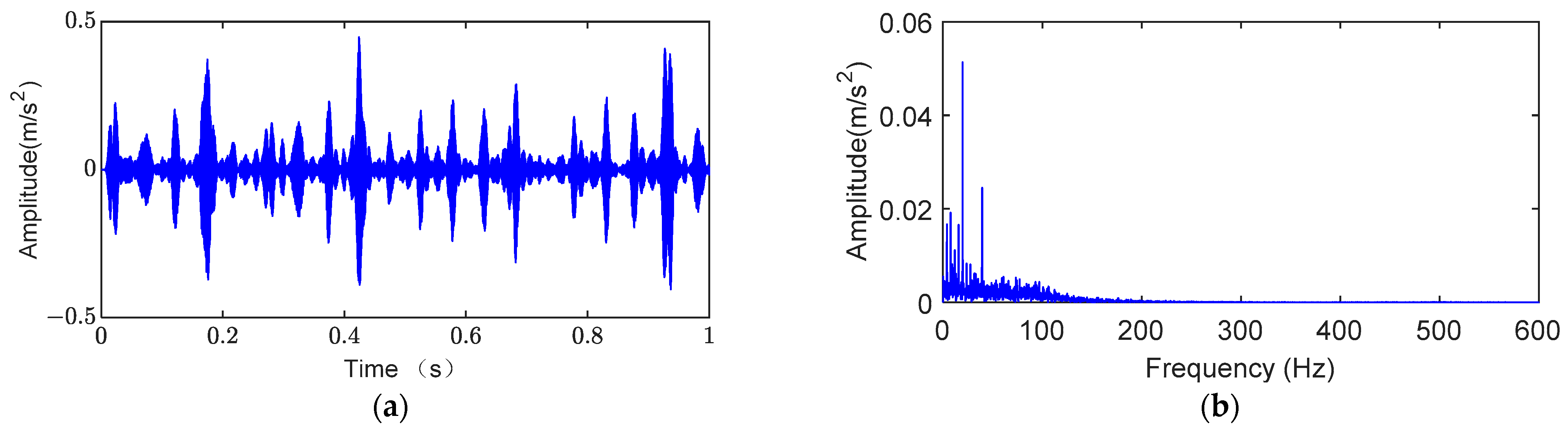
4.3. Inner Ring Failure Analysis

Firstly, the signals of some normal bearings and some inner ring faulty bearings are collected at a constant speed of 1200 rpm. The time-domain diagram is shown in Figure 12. Then, the signals of the inner ring faulty bearings are collected and analyzed using the proposed method in this paper.

Utilizing the collected normal and faulty signals, this study crafted an optimal weight spectrum, illustrated in Figure 13. Following this, the signal designated for analysis underwent decomposition via Symplectic Geometric Modal Decomposition (SGMD), with the decomposition’s parameters determined based on empirical evidence. The outcomes of this decomposition process are captured in Figure 14a, while Figure 14b delineates the normalized spectrum associated with each of the decomposition’s components. Subsequent to this, the optimal weight spectrum index for each of the Symplectic Geometry Components (SGCs) was computed, as depicted in Figure 15. Among these components, the 6th SGC was identified as bearing the highest optimal weight spectral index, marking it as the fault-sensitive component; the time-domain diagram is shown in Figure 16a. An envelope spectrum analysis of this fault-sensitive signal, presented in Figure 16b, revealed the fault characteristic frequency $f_i$ along with the multiplicative frequency of the inner ring. When the inner ring is damaged, because the relative position of the damage point and the load changes periodically, the vibration amplitude changes periodically when the collision occurs, showing an amplitude modulation phenomenon. This modulation is related to the speed of the rotating shaft. The failure frequency of the bearing and the side frequency of the rotating speed can be clearly seen in the envelope spectrum of Figure 16b. These results are used in the diagnosis of a fault within the bearing’s inner ring, confirming the effectiveness of the proposed methodology in identifying and diagnosing fault characteristics accurately.

This process underscores the proposed method’s capability to discern and highlight fault-sensitive components through SGMD, guided by an optimal weight spectrum derived from historical data. The ability to isolate and analyze these components further enables the precise identification of fault types, such as those occurring in the inner ring of a bearing, facilitating accurate fault diagnosis. The methodology’s success in pinpointing the fault characteristic frequency and its multiplicative frequencies demonstrates its potential as a robust tool for fault analysis in mechanical systems.

To highlight the efficacy of the proposed method, it is contrasted with other prevalent fault diagnosis techniques, namely Feature Mode Decomposition (FMD), Variational Mode Decomposition (VMD), and spectral kurtosis, referred to here as spectral kurtosis for its ability to identify peaks in the frequency spectrum.

For the application of FMD, a filter length of L = 30 was chosen, and the number of modes to be decomposed was set to equal the number of identified faults, n = 1, with additional parameter settings adhering to those outlined in the referenced literature [34]. The outcomes, depicted in Figure 17, failed to reveal the eigenfrequency of the outer ring fault and its corresponding correlation frequency. This discrepancy suggests that the FMD principle, which aims to isolate the component with the highest correlation kurtosis, might not effectively discern fault components when they are submerged within the noise across the entire spectrum. Consequently, the component identified as having the highest correlation may not be related to the fault, leading to unsatisfactory diagnostic results when following the parameter selection recommended in the literature [34].

This comparison underscores the advantages of the proposed SGMD-based method, which guided by the optimal weight spectrum demonstrates superior capability in accurately identifying fault-sensitive components amidst noise. Unlike FMD, which relies on the correlation kurtosis principle and may inadvertently highlight irrelevant components, the proposed method utilizes a targeted approach to discern fault characteristics, thereby offering a more reliable diagnostic tool. This distinction highlights the importance of selecting an appropriate diagnostic methodology that can adeptly navigate the challenges posed by noise and other interferences in the signal analysis.

The decomposition result of VMD is shown in Figure 18 below, and then the kurtosis index of each component signal is calculated as shown in Figure 19a, and the signal with the largest kurtosis is treated as the sensitive component, and the final result is shown in Figure 19b. From the final result, no fault information is extracted.

Figure 20a shows the spectral kurtosis result and Figure 20b shows the envelope spectrum after spectral kurtosis filtering. From the final results, both the transconductance and its multiplicative frequency are derived, but the conclusion is not reliable.

In order to demonstrate the advantages of this article more intuitively, the results of comparing the proposed method with other methods are shown in

Table 3. Comparison of results from different methods.

Methods	Inner Ring Failure	Outer Ring Failure
Proposed method	√	√
FMD	×	×
VMD	×	×
Spectral kurtosis	×	×

(√ indicates successful diagnosis, × is the opposite).

5. Conclusions

This study introduces a fault diagnosis methodology that utilizes Symplectic Geometric Modal Decomposition (SGMD) guided by an optimal weight spectrum. This optimal weight spectrum is obtained through convex optimization of normal and fault signals, allowing for a clear differentiation between fault and interference components. This framework effectively guides the SGMD process in selecting fault-sensitive components, ensuring a targeted approach to fault diagnosis. Experimental validations demonstrate the robust performance and superiority of the method compared to established techniques such as Feature Mode Decomposition (FMD), Variational Mode Decomposition (VMD), and spectral kurtosis. The proposed method’s ability to accurately identify fault-sensitive components suggests its potential as a powerful tool in fault diagnosis. However, the methodology presented here operates under the assumption of constant speed conditions when generating the optimal weight spectrum. This limitation indicates that the current approach may not fully consider the complexities associated with variable speed conditions, which are common in real-world scenarios and can significantly impact the diagnosis of mechanical faults. Future research will focus on extending the method’s applicability to variable speed conditions in order to refine the diagnostic process further and ensure its effectiveness across a wider range of operational scenarios, thereby increasing its utility and relevance in practical applications.

References

1. Zhou, P.; Chen, S.; He, Q.; Wang, D.; Peng, Z. Rotating machinery fault-induced vibration signal modulation effects: A review with mechanisms, extraction methods and applications for diagnosis. Mech. Syst. Signal Process. 2023, 200, 110489. [Google Scholar] [CrossRef]
2. Kong, X.; Li, X.; Zhou, Q.; Hu, Z.; Shi, C. Attention Recurrent Autoencoder Hybrid Model for Early Fault Diagnosis of Rotating Machinery. IEEE Trans. Instrum. Meas. 2021, 70, 2505110. [Google Scholar] [CrossRef]
3. Hong, Y.; Kim, M.; Lee, H.; Park, J.J.; Lee, D. Early Fault Diagnosis and Classification of Ball Bearing Using Enhanced Kurtogram and Gaussian Mixture Model. IEEE Trans. Instrum. Meas. 2019, 68, 4746–4755. [Google Scholar] [CrossRef]
4. Li, Y.; Yang, Y.; Wang, X.; Liu, B.; Liang, X. Early fault diagnosis of rolling bearings based on hierarchical symbol dynamic entropy and binary tree support vector machine. J. Sound Vib. 2018, 428, 72–86. [Google Scholar] [CrossRef]
5. Qin, Y. A New Family of Model-Based Impulsive Wavelets and Their Sparse Representation for Rolling Bearing Fault Diagnosis. IEEE Trans. Ind. Electron. 2018, 65, 2716–2726. [Google Scholar] [CrossRef]
6. Li, Z.; Gao, J.; Li, H.; Zhang, Z.; Liu, N.; Zhu, X. Synchroextracting transform: The theory analysis and comparisons with the synchrosqueezing transform. Signal Process. 2020, 166, 107243. [Google Scholar] [CrossRef]
7. Yu, G.; Huang, X.; Lin, T.; Dong, H. A non-linear time–frequency tool for machinery fault diagnosis under varying speed condition. Mech. Syst. Signal Process. 2023, 186, 109849. [Google Scholar] [CrossRef]
8. Dong, H.; Yu, G.; Lin, T.; Li, Y. An energy-concentrated wavelet transform for time-frequency analysis of transient signal. Signal Process. 2023, 206, 108934. [Google Scholar] [CrossRef]
9. Yu, G. A Concentrated Time-Frequency Analysis Tool for Bearing Fault Diagnosis. IEEE Trans. Instrum. Meas. 2019, 69, 371–381. [Google Scholar] [CrossRef]
10. Miao, Y. Automatic instantaneous frequency estimator for multicomponent signals with the variable number of components. Signal Process. 2022, 197, 108541. [Google Scholar] [CrossRef]
11. Wang, H.; Chen, S.; Zhai, W. Data-driven adaptive chirp mode decomposition with application to machine fault diagnosis under non-stationary conditions. Mech. Syst. Signal Process. 2023, 188, 109997. [Google Scholar] [CrossRef]
12. Zhang, Y.; Xing, K.; Bai, R.; Sun, D.; Meng, Z. An enhanced convolutional neural network for bearing fault diagnosis based on time–frequency image. Measurement 2020, 157, 107667. [Google Scholar] [CrossRef]
13. Xia, S.; Zhang, J.; Ye, S.; Xu, B.; Xiang, J.; Tang, H. A mechanical fault detection strategy based on the doubly iterative empirical mode decomposition. Appl. Acoust. 2019, 155, 346–357. [Google Scholar] [CrossRef]
14. Lazhari, M.; Sadhu, A. Decentralized modal identification of structures using an adaptive empirical mode decomposition method. J. Sound Vib. 2019, 447, 20–41. [Google Scholar] [CrossRef]
15. Zhao, H.W.; Huang, N.E. Ensemble empirical mode decomposition: A noise-assisted data analysis method. Adv. Adaptive Data Anal. 2009, 1, 1–41. [Google Scholar]
16. Lei, Y.; He, Z.; Zi, Y. Application of the EEMD method to rotor fault diagnosis of rotating machinery. Mech. Syst. Signal Process. 2009, 23, 1327–1338. [Google Scholar] [CrossRef]
17. Li, H.; Liu, T.; Wu, X.; Li, S. Research on test bench bearing fault diagnosis of improved EEMD based on improved adaptive resonance technology. Measurement 2021, 185, 109986. [Google Scholar] [CrossRef]
18. Yan, R.; Gao, R.X.; Chen, X. Wavelets for fault diagnosis of rotary machines: A review with applications. Signal Process. 2014, 96, 1–15. [Google Scholar] [CrossRef]
19. Chen, J.; Li, Z.; Pan, J.; Chen, G.; Zi, Y.; Yuan, J.; Chen, B.; He, Z. Wavelet transform based on inner product in fault diagnosis of rotating machinery: A review. Mech. Syst. Signal Process. 2016, 70–71, 1–35. [Google Scholar] [CrossRef]
20. Kankar, P.K.; Sharma, S.C.; Harsha, S.P. Rolling element bearing fault diagnosis using wavelet transform. Neurocomputing 2011, 74, 1638–1645. [Google Scholar] [CrossRef]
21. Wang, Z.; Yang, N.; Li, N.; Du, W.; Wang, J. A new fault diagnosis method based on adaptive spectrum mode extraction. Struct. Health Monit. 2021, 20, 3354–3370. [Google Scholar] [CrossRef]
22. Wang, Z.; Du, W.; Wang, J.; Zhou, J.; Han, X.; Zhang, Z.; Huang, L. Research and application of improved adaptive MOMEDA fault diagnosis method. Measurement 2019, 140, 63–75. [Google Scholar] [CrossRef]
23. Sun, Y.; Jian, M.; Zhang, X.; Dong, J.; Shen, L.; Chen, B. Reconstruction of normal and albedo of convex Lambertian objects by solving ambiguity matrices using SVD and optimization method. Neurocomputing 2016, 207, 95–104. [Google Scholar] [CrossRef]
24. Zhang, Z.; Liu, B.; Liu, Y.; Zhang, H. Fault Feature-Extraction Method of Aviation Bearing Based on Maximum Correlation Re’nyi Entropy and Phase-Space Reconstruction Technology. Entropy 2022, 24, 1459. [Google Scholar] [CrossRef] [PubMed]
25. Yang, M.; Xu, Y.; Zhang, K.; Zhang, X. Singular component decomposition and its application in rolling bearing fault diagnosis. Meas. Sci. Technol. 2024, 35, 015120. [Google Scholar] [CrossRef]
26. Wang, Y.; Markert, R.; Xiang, J.; Zheng, W. Research on variational mode decomposition and its application in detecting rub-impact fault of the rotor system. Mech. Syst. Signal Process. 2015, 60–61, 243–251. [Google Scholar] [CrossRef]
27. Dragomiretskiy, K.; Zosso, D. Variational Mode Decomposition. IEEE Trans. Signal Process. 2014, 62, 531–544. [Google Scholar] [CrossRef]
28. Lian, J.; Liu, Z.; Wang, H.; Dong, X. Adaptive variational mode decomposition method for signal processing based on mode characteristic. Mech. Syst. Signal Process. 2018, 107, 53–77. [Google Scholar] [CrossRef]
29. Li, J.; Yao, X.; Wang, H.; Zhang, J. Periodic impulses extraction based on improved adaptive VMD and sparse code shrinkage denoising and its application in rotating machinery fault diagnosis. Mech. Syst. Signal Process. 2019, 126, 568–589. [Google Scholar] [CrossRef]
30. Randall, R.B.; Antoni, J. Rolling element bearing diagnostics—A tutorial. Mech. Syst. Signal Process. 2011, 25, 485–520. [Google Scholar] [CrossRef]
31. Endo, H.; Randall, R.B. Enhancement of autoregressive model based gear tooth fault detection technique by the use of minimum entropy deconvolution filter. Mech. Syst. Signal Process. 2007, 21, 906–919. [Google Scholar] [CrossRef]
32. McDonald, G.L.; Zhao, Q.; Zuo, M.J. Maximum correlated Kurtosis deconvolution and application on gear tooth chip fault detection. Mech. Syst. Signal Process. 2012, 33, 237–255. [Google Scholar] [CrossRef]
33. Lyu, X.; Hu, Z.; Zhou, H.; Wang, Q. Application of improved MCKD method based on QGA in planetary gear compound fault diagnosis. Measurement 2019, 139, 236–248. [Google Scholar] [CrossRef]
34. Miao, Y.; Zhang, B.; Li, C.; Lin, J.; Zhang, D. Feature Mode Decomposition: New Decomposition Theory for Rotating Machinery Fault Diagnosis. IEEE Trans. Ind. Electron. 2023, 70, 1949–1960. [Google Scholar] [CrossRef]
35. Miao, Y.; Zhang, B.; Lin, J.; Zhao, M.; Liu, H.; Liu, Z.; Li, H. A review on the application of blind deconvolution in machinery fault diagnosis. Mech. Syst. Signal Process. 2022, 163, 108202. [Google Scholar] [CrossRef]
36. Lee, J.; Liu, Y.; Yu, L. SGST: An Open Source Semantic Geostreaming Toolkit. In Proceedings of the 2011 ACM SIGSPATIAL International Workshop on GeoStreaming, IWGS 2011, Chicago, IL, USA, 1 November 2011; Volume 1, pp. 17–20. [Google Scholar]
37. Cheng, J.; Yang, Y.; Hu, N.; Cheng, Z.; Cheng, J. A noise reduction method based on adaptive weighted symplectic geometry decomposition and its application in early gear fault diagnosis. Mech. Syst. Signal Process. 2021, 149, 107351. [Google Scholar] [CrossRef]
38. Pan, H.; Yang, Y.; Li, X.; Zheng, J.; Cheng, J. Symplectic geometry mode decomposition and its application to rotating machinery compound fault diagnosis. Mech. Syst. Signal Process. 2019, 114, 189–211. [Google Scholar] [CrossRef]
39. Hou, B.; Wang, D.; Kong, J.; Liu, J.; Peng, Z.; Tsui, K. Understanding importance of positive and negative signs of optimized weights used in the sum of weighted normalized Fourier spectrum/envelope spectrum for machine condition monitoring. Mech. Syst. Signal Process. 2022, 174, 109094. [Google Scholar] [CrossRef]
40. Hou, B.; Wang, D.; Peng, Z.; Tsui, K. Adaptive Fault Components Extraction by Using an Optimized Weights Spectrum Based Index for Machinery Fault Diagnosis. IEEE Trans. Ind. Electron. 2024, 71, 985–995. [Google Scholar] [CrossRef]
Figure 1. The flow chart of proposed method.
Symmetry 16 00408 g001
Figure 2. Experimental platform diagram: (a) QPZZ-II experimental platform, (b) inner ring fault bearing, (c) outer ring fault bearing.
Symmetry 16 00408 g002
Figure 3. Time-domain diagram of bearing signal: (a) healthy bearing signal, (b) outer ring faulty bearing signal.
Symmetry 16 00408 g003
Figure 4. Optimal weight spectrum.
Symmetry 16 00408 g004
Figure 5. SGMD decomposition results: (a) time-domain signal of SGCs, (b) frequency spectrum of SGCs.
Symmetry 16 00408 g005
Figure 6. Optimal weight spectrum index chart.
Symmetry 16 00408 g006
Figure 7. Diagnostic results of the proposed method: (a) sensitive component, (b) envelope spectrum of sensitive components.
Symmetry 16 00408 g007
Figure 8. Results of FMD decomposition: (a) FMD final component, (b) envelope spectrum of FMD final component.
Symmetry 16 00408 g008
Figure 9. VMD decomposition results: (a) time-domain signal of IMFs, (b) frequency spectrum of IMFs.
Symmetry 16 00408 g009
Figure 10. Analysis results of VMD: (a) the kurtosis of each component in VMD, (b) envelope spectrum of VMD sensitive components.
Symmetry 16 00408 g010
Figure 11. Analysis results of spectral kurtosis: (a) spectral kurtosis, (b) envelope spectrum after spectral kurtosis filtering.
Symmetry 16 00408 g011
Figure 12. Time-domain diagram of bearing signal: (a) healthy bearing signal, (b) inner ring faulty bearing signal.
Symmetry 16 00408 g012
Figure 13. Optimal weight spectrum.
Symmetry 16 00408 g013
Figure 14. SGMD decomposition results: (a) time-domain signal of SGCs, (b) frequency spectrum of SGCs.
Symmetry 16 00408 g014
Figure 15. Optimal weight spectrum index chart.
Symmetry 16 00408 g015
Figure 16. Diagnostic results of the proposed method: (a) sensitive component, (b) envelope spectrum of sensitive components.
Symmetry 16 00408 g016
Figure 17. Results of FMD decomposition: (a) FMD final component, (b) envelope spectrum of FMD final component.
Symmetry 16 00408 g017
Figure 18. VMD decomposition results: (a) time-domain signal of IMFs, (b) frequency spectrum of IMFs.
Symmetry 16 00408 g018
Figure 19. Analysis Results of VMD: (a) the kurtosis of each component in VMD, (b) envelope spectrum of VMD sensitive components.
Symmetry 16 00408 g019
Figure 20. Analysis results of spectral kurtosis: (a) spectral kurtosis, (b) envelope spectrum after spectral kurtosis filtering.
Symmetry 16 00408 g020