Article

The Quantum Ratio

by
Kenichi Konishi
1,2,* and
Hans-Thomas Elze
1
1
Department of Physics “E. Fermi”, University of Pisa, Largo Pontecorvo 3, Ed. C, 56127 Pisa, Italy
2
INFN, Pisa Section, Largo Pontecorvo 3, Ed. C, 56127 Pisa, Italy
*
Author to whom correspondence should be addressed.
Symmetry 2024, 16(4), 427; https://doi.org/10.3390/sym16040427
Submission received: 21 February 2024 / Revised: 29 March 2024 / Accepted: 1 April 2024 / Published: 4 April 2024
(This article belongs to the Special Issue Quantum Mechanics: Concepts, Symmetries, and Recent Developments)

Abstract

:
The concept of quantum ratio has emerged from recent efforts to understand how Newton’s equations appear for the center of mass (CM) of an isolated macroscopic body at finite body temperatures as a first approximation of quantum mechanical equations. It is defined as Q R q / L 0 , where the quantum fluctuation range R q is the spatial extension of the pure-state CM wave function, whereas L 0 stands for the body’s linear size (the space support of the internal bound-state wave function). The two cases R q / L 0 1 and R q / L 0 1 roughly correspond to the body’s CM behaving classically or quantum mechanically, respectively. In the present note, we elaborate on this concept and illustrate it through several examples. An important notion following from introduction of the quantum ratio is that the elementary particles (thus, the electron and the photon) are quantum mechanical even when environment-induced decoherence places them into a mixed state. Thus, decoherence and classical state should not be identified. This simple observation, further illustrated by consideration of a few atomic and molecular processes, may have significant implications for the way that quantum mechanics works in biological systems.

1. Introduction: The Quantum Ratio

The concept of quantum ratio emerged during the efforts to understand the conditions under which the center of mass (CM) of an isolated macroscopic body possesses a unique classical trajectory. It is defined as
Q R q L o ,
where R q is the quantum fluctuation range of the CM of the body under consideration and L 0 is the body’s (linear) size. The criterion proposed to tell whether the body behaves quantum mechanically or classically is [1]
Q 1 , ( quantum ) ,
or
Q 1 , ( classical ) ,
respectively.
Let us assume that the total wave function of the body has a factorized form
Ψ ( r 1 , r 2 , r N ) = Ψ C M ( R ) ψ i n t ( r ^ 1 , r ^ 2 , r ^ N 1 ) ,
where Ψ C M is the CM wave function, the N-body bound state is described by the internal wave function ψ i n t , { r ^ 1 , r ^ 2 , r ^ N 1 } are the internal positions of the component atoms or molecules, R is the CM position, and r i = R + r ^ i ( i = 1 , 2 , , N ). In the case of a macroscopic body, N can be as large as N 10 25 , 10 50 , etc.

1.1. The Size of the Body

L 0 is determined by ψ i n t . A possible definition of L 0 is
L 0 = Max i r ¯ i , r ¯ i ( ψ i n t | ( r ^ i ) 2 | ψ i n t ) 1 / 2 ,
though the detailed definition is not important here. L 0 is the spatial support (extension) of the internal wave function describing the bound state a macroscopic body, and from some scales upwards, might well be described as a classical bound state due to gravitational or electromagnetic forces; however, their size is always well defined). It is the (linear) size of the body. Even though L 0 might somewhat depend on the body temperature T (the average internal excitation energy), it is well defined even in the T 0 limit. It represents the extension of the ground-state wave function of the bound state describing the body.
For an atom, the definition (5) correctly provides the outermost orbit in the electronic configuration. L 0 varies from 0.5 Å to hundreds of Å for atoms and molecules. The atomic nuclei (composed of protons and neutrons), which are bound more strongly by short-range nuclear forces, have smaller size L 0 on the order of Fermi ∼ 10 13 cm. For mesoscopic to macroscopic bodies, L 0 varies vastly depending on the composition, the types of the forces which bind them, and their particular molecular or crystalline structures. For the earth (the radius) L 0 6400 km.
An exception is the case of the elementary particles, which have L 0 = 0 . This has a simple implication according to (2): having Q = , the elementary particles are quantum-mechanical.
It might be argued that length scales (i.e., small or large) are relative concepts in physics; at distances much larger than L 0 , any body looks pointlike. More generally, when changing the scales of distances or energies, the physics might look similar. A more rigorous formulation of this idea (scale invariance) is that of the renormalization group in relativistic quantum field theories in four dimensions, e.g., theories of the fundamental interactions [2,3,4,5]), or in lower-dimensional models of critical phenomena [6].
Scale invariance holds if the system possesses no fixed length scale (nonrelativistic quantum mechanics, having only ħ with the dimension of an action as the fundamental constant in its formulation, shares this property [7]). The so-called quantum nonlocality is one of its consequences. However, in specific problems the masses and the potential explicitly break scale invariance in general. For a class of potentials, such as the delta-function or 1 / r 2 potentials in D = 2 space dimensions, the system possesses exact scale invariance [8]. From the point of view of the theory of fundamental interactions, the absence of a fixed length scale means that physics at low energies does not depend on the ultraviolet cutoff Λ . Thus, we need to introduce the regularization (and renormalization) of the theory because of the presence of ultraviolet divergences. In other words, the theory is of renormalizable type, that is, a quantum field theory without any a priori mass (or length) parameter.
For the questions of interest in the present work, however, it is important, and we do know, that the world we live in has definite length scales, such as Bohr’s radius and the size of atomic nuclei. In other words, terms such as microscopic (from elementary particles and nuclei to atoms and molecules) and macroscopic (much larger than these) have well-defined concrete meanings.
These fixed sizes (or length scales) characterizing our world are set by the fundamental constants of nature (ħ, e, c) and by the parameters in the theory of the fundamental (strong and electroweak) interactions [2,3,4,5], namely, the quark and lepton masses, W and Z masses. See Section 2.1 for more on this topic.

1.2. Quantum Range R q

The quantum fluctuation range R q is determined by Ψ C M ( R ) . In principle, it is just the (spatial) extension of the pure-state wave function Ψ C M ( R ) describing the CM of the body. However, it is a much more complex quantity than L 0 , and depends on many factors. In quantum mechanics (QM) there is no a priori upper limit to R q . Take for instance the wave function of a free particle, ψ ; while it might be thought that the normalization condition | | ψ | | = 1 necessarily sets a finite quantum fluctuation range, this is not the case. As is well known (Weyl’s criterion), a particle can be in a state arbitrarily close to a plane-wave state,
ψ e i p · r / ħ ,
i.e., in a momentum eigenstate, which has R q = . This fact, the absence of a priori upper limit for R q , is another consequence of the fact that QM laws contain no fundamental constant with the dimension of a length.
Given a body, R q will in general depend on the internal structures, excitation modes, and body temperature. These cause self-induced (or thermal) decoherence due to the emission of photons which carry away information and seriously reduce R q . If the body is not isolated, its R q is severely affected by the action of environment-induced decoherence [9,10,11,12,13,14] upon the surrounding temperature, flux, etc. Moreover, R q depends on the external electromagnetic fields, which may split the wave packets, as in the Stern–Gerlach setup, as well as on possible quantum-mechanical correlations (entanglement) among distant particles. R q may depend also on time.
An important question concerns the width of the wave packet of the CM of an isolated (microscopic or macroscopic) particle, Δ C M . This should not be confused with L 0 . Being the spread of a single-particle wave function, Δ C M is a measure of the quantum fluctuation range
R q Δ C M ,
though R q can be much larger than Δ C M in general.
As for the relation between Δ C M and L 0 , Δ C M corresponds to the uncertainty of the CM position of the body. For a macroscopic body, an experimentalist who is capable of measuring and determining its size L 0 with some precision will certainly be able to measure the CM position R with
Δ C M L 0 , or even with Δ C M L 0 .
Nevertheless, such a relation neither holds necessarily nor is required in general.
A macroscopic body, especially at exceedingly low temperatures near T = 0 , may well be in a state of position uncertainty (the width of the wave packet)
Δ C M L 0 .
Using (7), such a system is seen to have Q 1 , and as such is quantum mechanical. Many attempts to realize macroscopic quantum states experimentally by bringing the system temperatures close to T = 0 have been made recently [15,16,17,18,19,20,21,22,23,24,25,26].
Vice versa, a well-defined CM position (8) set up at time t = 0 does not in itself tell whether the system will behave quantum mechanically or classically.
A free wave packet of an atom or molecule with initial position uncertainty Δ C M will quickly diffuse (the diffusion rate depends on the mass) and acquire R q Δ C M L 0 (see Table 1, taken from [1]). In the Stern–Gerlach setup, with an inhomogeneous magnetic field, the (transverse) wave packet of an atom or a molecule with spin will be split in two or more wave packets, which can become separated even by a macroscopic distance ( R q ) such that R q L 0 , Q 1 (see Section 2.3 for more about this).
On the other hand, a macroscopic body does not diffuse (see Table 1). Its CM wave packet does not split under an inhomogeneous magnetic field either [1]. Therefore, if the CM position of a macroscopic body is measured with precision (8) at time t = 0 , the relation R q L 0 ( Q 1 ) is maintained in time. Such a body evolves classically with a well-defined trajectory obeying Newton’s equations [1].

1.3. The Microscopic Degrees of Freedom Inside of a Macroscopic Body Are Quantum Mechanical

The present discussion on the quantum ratio is concerned with the question of how classical behavior for the CM of a macroscopic body emerges from QM. An important fact to be kept in mind is the following: even if a macroscopic (or a mesoscopic) body might behave classically as a whole due to environment-induced or self-induced (or thermal) decoherence and to its large mass [1], the internal microscopic degrees of freedom, electrons, atomic nuclei, and photons remain quantum mechanical (see Section 2.1, Section 2.2 and Section 3). All sorts of quantum-mechanical processes (e.g., tunneling) continue to be active inside the body, even if various decoherence effects may be significant. These quantum phenomena constitute the essence of the physics of polymers and general macromolecules, and consequently of biology. They hold the key to the answers to many questions in biology, genetics, and neuroscience that are unanswered today (see for instance [27,28]). The consideration of the present note has nothing to add directly to these questions; however, see a few related general comments in Section 3 below.

2. The Quantum Ratio Illustrated

In this section, the quantum ratio is illustrated via several examples.

2.1. Elementary Particles

The elementary particles known today (as of the year 2024, see [29]) are the quarks, leptons (electron, muon, τ lepton), the three types of neutrinos, and the gauge bosons (the gluons, W, Z bosons, and photon), with the masses listed below (Table 2, Table 3 and Table 4).
The fact that the processes involving these particles are very accurately described by the local quantum field theory S U ( 3 ) Q C D × { S U ( 2 ) L × U ( 1 ) } G W S up to the energy range of O ( 10 ) TeV means that
L 0 O ( 10 18 ) cm .
In future, these elementary particles might well turn out to be made of some constituents unknown today, bound by some new forces yet to be discovered. For present-day physics, their size can be taken to be
L 0 = 0 . . . Q = .
Thus, the elementary particles are quantum mechanical. The virtual emission and absorption of a particle of mass m provides the physical “size” h / m c , known as the Compton length, of any quantum-mechanical particle; however, this should be distinguished from the size L 0 defined as the extension of its internal wave function.
This notion is generally taken for granted by physicists, even if no justification is (was) known as such. Here, as we are inquiring as to whether a certain “particle”, be it an atom, molecule, macromolecule, a piece of crystal, etc., behaves quantum mechanically or classically, and under which conditions, it perhaps makes sense to ask whether or why an elementary particle is quantum mechanical. Introduction of the quantum-ratio criterion offers an immediate (affirmative) answer to the first question and explains the second. By definition, the elementary particles have no internal structures, and consequently no internal excitations. Thus, there is no sense in talking about their body temperature or thermal decoherence.
Note that any quantum particle, such as an electron, behaves “classically” under certain conditions (the Ehrenfest theorem), e.g., when it is well-localized, free or under homogeneous electromagnetic field, and within the diffusion time; however, this is not what we mean by a classical particle.
The observation that the elementary particles (Table 2, Table 3 and Table 4) are quantum mechanical in the light of the quantum ratio (10) and (11) might sound new; however, it is really not. Actually, it reflects the common understanding that matured around 1970 in the high-energy physics community (e.g., ‘t Hooft, Cargese lecture [30]) that the laws of nature at the microscopic level are expressed by a renormalizable and relativistic local gauge theory (a quantum field theory) of the elementary particles. Such a theory describes pointlike particles ( L 0 = 0 ). Quantum gravity or string theory effects, possibly relevant near the Planckian energies M P l 10 19 GeV , do contain a length scale ∼ 10 32 cm, but it is beyond the scope of the present work to consider whether and how these affect the discussion of quantum or classical physics at the larger distances (≥ 10 18 cm) that we are concerned with here.
The scale or dilatation-invariance of this type of theories is broken by the necessity of introducing an ultraviolet cutoff, a mass scale Λ U V , to regularize, renormalize, and define a finite theory (quantum anomaly). Remarkably, the scale invariance is restored by the introduction of the renormalized coupling constants (defined conveniently at some reference mass scale μ ) and by giving them an appropriate μ dependence (the renormalization-group equations); see, e.g., Coleman’s 1971 Erice lecture [31].
The fixed length or mass scales of our world, mentioned in Section 1.1, concern the infrared fate of such dilatation invariance. These fixed scales can ultimately be traced to (i) the vacuum expectation value ϕ 0 246 GeV of the Higgs scalar field in the S U ( 2 ) × U ( 1 ) Glashow–Weinberg–Salam electroweak theory, and (ii) the mass scale Λ Q C D 150 MeV , dynamically generated by the strong interactions (quantum chromodynamics). These break scale-invariance. All fixed length scales, from the microscopic to the macroscopic world we live in, follow from these and from some dimensionless coupling constants in the S U ( 3 ) Q C D × { S U ( 2 ) × U ( 1 ) } G W S theory; for instance, the nuclear size is typically on the order of the pion’s Compton length, h / m π c , and m π 2 m u , d Λ Q C D . The proton and neutron masses (∼940 MeV/ c 2 ) are mainly provided by the strong interaction effects Λ Q C D . The Bohr radius is ħ 2 / m e e 2 .

2.2. Hadrons and Atomic Nuclei

Atomic nuclei, together with various hadrons (the mesons and baryons), are the smallest composite particles known today. Until around 1960, the mesons ( π , K, …) and baryons (p, n, …) used to be part of the list of “elementary particles”, together with leptons. As the theory of strong interactions (the quark model, and subsequently quantum chromodynamics, a non-Abelian S U ( 3 ) gauge theory of quarks and gluons) was established around 1974–1980, they were replaced by the quarks and gluons as more fundamental constituents of nature.
The atomic nuclei are bound states of the nucleons, i.e., protons (p) and neutrons (n). They are bound by the strong interactions, and their size is on the order of
L 0 A 1 / 3 fm , 1 fm 10 13 cm = 10 5 ,
where A is the mass number. The Coulombic wave functions in the atoms and molecules have extension ( R q ) of the order of Å; thus,
Q = R q L 0 O ( 10 5 ) .
The atomic nuclei are quantum mechanical.
To say that the atomic nuclei are quantum mechanical because of the atomic extension (13), however, is certainly too reductive. The atomic nuclei indeed may appear without being bound in atoms. For instance, the α particle is the nucleus of the helium atom, but may come out of a metastable nucleus through α decay and propagate as a free particle. It possesses a size on the order of (12), much larger than the typical size of an elementary particles (10), but for processes typically involving the distance scales much larger than 1 fm, it behaves as a pointlike particle, i.e., quantum mechanically, just as any elementary particle does. Similarly for the proton, the nucleus of the hydrogen atom, with L 0 0.84 fm.

2.3. Stern–Gerlach Experiment

The next smallest composite particles known in nature are the atoms. They are Coulombic composite states made of electrons moving around a positively charged atomic nuclei, almost pointlike (at the atomic scales) and O ( 10 3 10 5 ) times heavier than the electron.
Let us consider the well known Stern–Gerlach process of atoms with a magnetic moment in an inhomogeneous magnetic field. To be concrete, we take as an example the very original Stern–Gerlach experiment with the silver atom [32] A g , with mass and size
m A g 1.79 × 10 22 g , L 0 1.44 × 10 8 cm .
With the electronic configuration and the global quantum number
[ K r ] 4 d 10 5 s 1 ,   2 S 1 / 2 ;
the magnetic moment of the atom is dominated by the spin of the outmost electron,
μ = e ħ 2 m e c g s ,
where g is the gyromagnetic ratio g 2 of the electron. [ K r ] above indicates the zero angular momentum-spin ( L = S = 0 ) closed shell of the Kripton electronic configuration describing the first 36 electrons.
The question is whether the silver atom, which is certainly a quantum-mechanical bound state of 47 electrons, 47 protons, and 51 neutrons and has a mass ∼100 times that of the hydrogen atom, behaves as a whole (i.e., its CM) as a QM particle with spin 1 / 2 or as a classical particle of magnetic moment μ .
The beam of A g is sent into the region, 3.5 cm long, of an inhomogeneous magnetic field B = ( 0 , 0 , B ( z ) ) , d B ( z ) / d z 0 , as it proceeds in, e.g., the x ^ direction. The beam width, which reflects the apertures of the two slits used to prepare the well-collimated beam, is about ∼ 0.02 0.03 mm wide (the transverse wave packet size of the atom can be taken to be of this order; the silver atom, having a mass roughly 100 times that of the hydrogen atom, has a diffusion time on the order of 10 2 s (see Table 1), meaning that the diffusion during the travel of 3.5 cm is entirely negligible). After passing the region of the magnetic field, the image of the atoms on the glass screen shows two bands clearly separated by about 0.2 mm in the direction of z ^ . In other words, at the end of the region with the magnetic field, the atom is described by a split wave packet of the form
ψ = ψ 1 ( r ) | + ψ 2 ( r ) |
with the centers of the two subpackets ψ 1 and ψ 2 at r = r 1 and r = r 2 , respectively, where | z 1 z 2 |   0.2 mm. The spatial support of the wave function ψ can be taken as about that size. It follows that
Q = R q L 0 0.2 mm 1.4 · 10 8 cm 10 6 1 ,
with the A g atom as a whole behaving as a perfectly quantum-mechanical particle.
Actually, the fact that the wave packets are divided in two by an inhomogeneous magnetic field does not necessarily mean that the system is in a pure state of the form (17); the wave function of the form (17) corresponds to a 100% polarized beam, where all incident atoms are in the same spin state
c 1 | + c 2 | = c 1 c 2 , | c 1 | 2 + | c 2 | 2 = 1 .
If the beam is partially polarized or unpolarized, the spin state is described by a density matrix ρ . The pure state (19) corresponds to the density matrix
ρ ( p u r e ) = | c 1 | 2 c 1 c 2 * c 2 c 1 * | c 2 | 2 ,
whereas a general mixed state is described by a generic Hermitian 2 × 2 matrix ρ with
Tr ρ = 1 , ρ i i 0 , i = 1 , 2 .
In an unpolarized beam, ρ = 1 2 1 .
What the Stern–Gerlach experiment measures is the relative frequency with which the atom arriving at the screen happens to have spin s z = 1 2 or spin s z = 1 2 . Let
Π = | | = 1 0 0 0 , Π = | | = 0 0 0 1
be the projection operators on the spin-up (down) states; according to QM, the relative intensities of the upper and lower blots on the screen are
Π ¯ = Tr Π ρ = ρ 11 ; Π ¯ = Tr Π ρ = ρ 22 , ρ 11 + ρ 22 = 1 .
The prediction about the relative intensities of the two narrow atomic image bands from the wave function (17) and from the density matrix (23) is in general indistinguishable, as is well known. In other words, what the Stern–Gerlach experiment shows is not whether the atom is in a pure state of the form (17) or in a generic (spin-) mixed state (23), but rather that the silver atom is a quantum mechanical particle.
Indeed, the prediction for a classical particle is qualitatively different. If classical, each atom would move depending on the orientation of its magnetic moment, tracing a well-defined trajectory
m r ˙ = p , d p x d t = d p y d t = 0 , d p z d t = F z = z μ · B .
It would arrive at some generic point on the screen. If the initial orientation of the magnetic moment were random, after many classical atoms had arrived they would leave a continuous band of atomic images, rather than two narrow well-separated bands, as has been experimentally observed and as QM predicts.
Vice versa, if the orientation of the magnetic moment/spin is fixed (and the same) for all incident atoms, then classical atoms will produce only one narrow band, whereas QM atoms will leave two separate image bands. These considerations clearly tell that the concepts of mixed state and classical particle should be distinguished. We extend these discussions further in Section 3, taking into account the effects of environment-induced decoherence as well as the large spin limit and their respective relations to the classical limit (24).

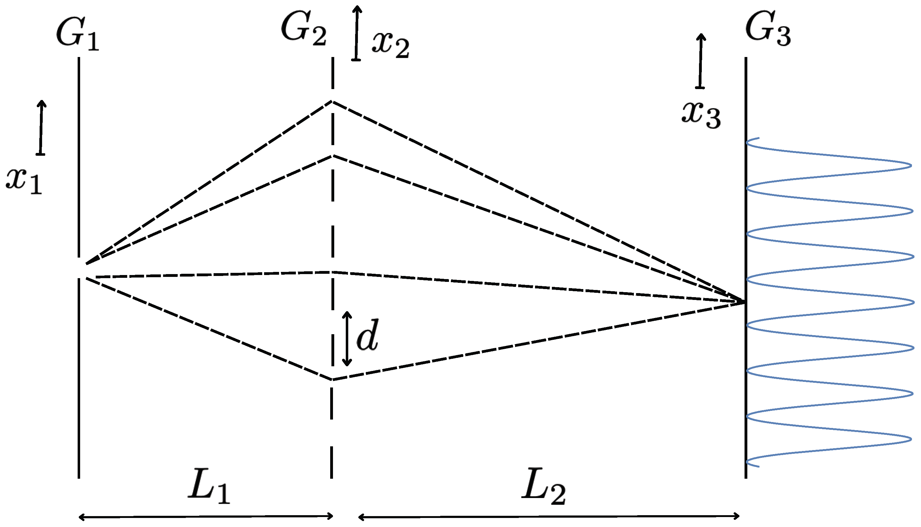
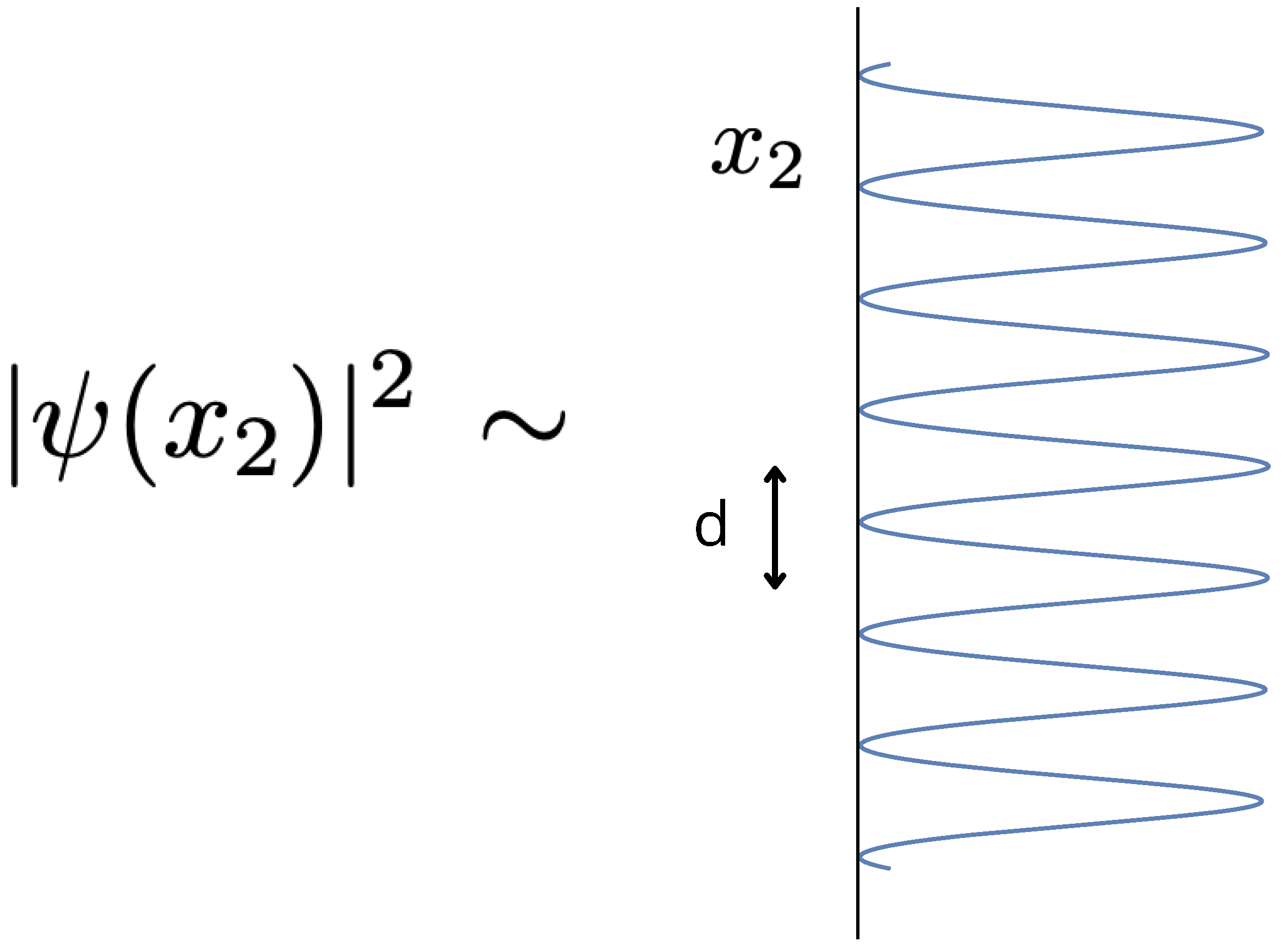
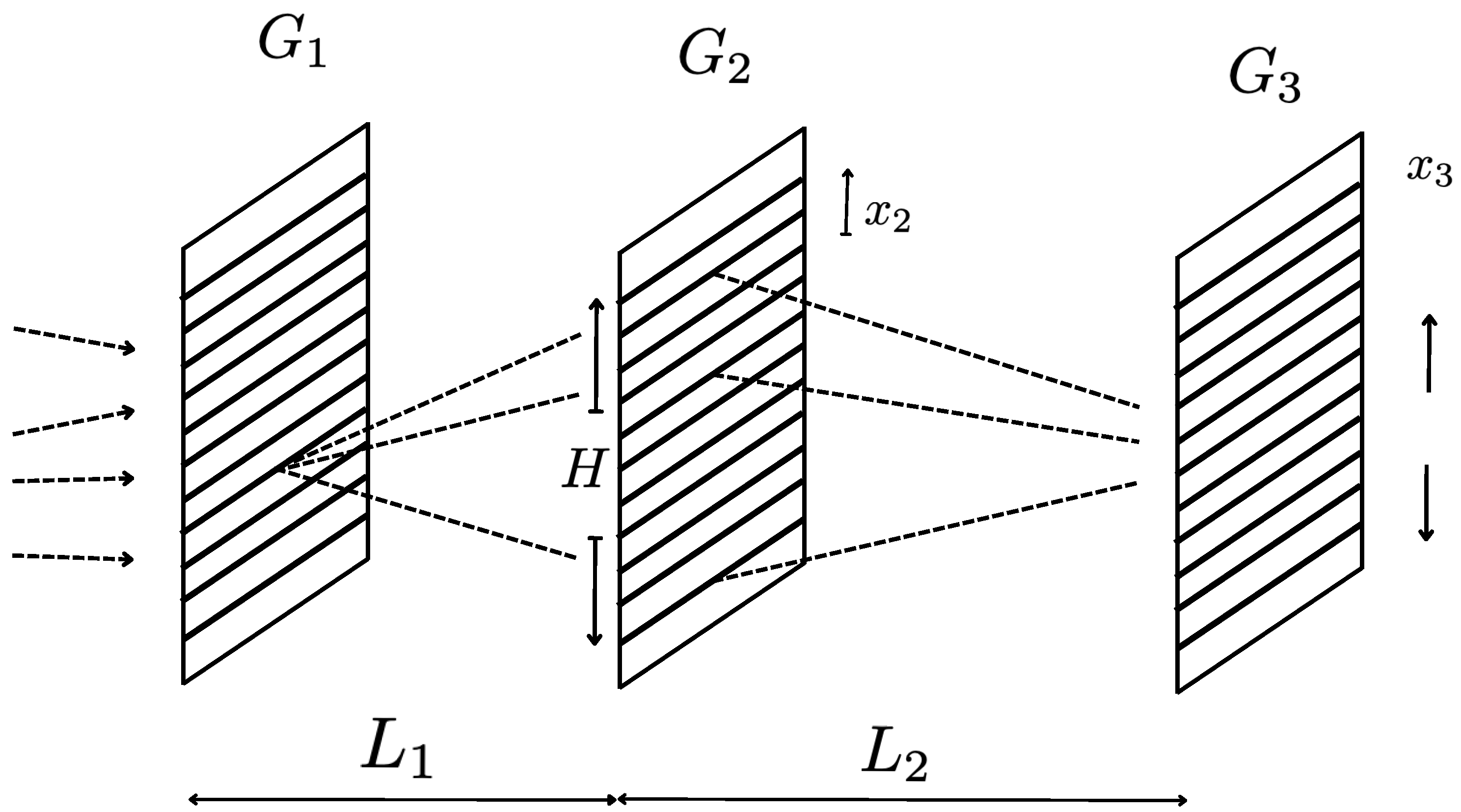
2.4. Atomic and Molecular Interferometry

Many beautiful experiments exhibiting the quantum mechanical feature (wave character) of atoms and molecules have been performed (or proposed) using various types of interferometers [33,34,35,36,37,38,39,40,41,42]. One of the most powerful approaches uses Talbot–Lau interferometry [33,36,37,38,39].
The essential part of all these experiments makes use of the so-called Talbot effect [43]. In a typical setting, an atomic or molecular beam passing through the first slit is sent to the diffraction grating ( G 2 in Figure 1), which consists of many slit apertures set with period d. After passing through the diffraction grating, the wave function of the atom or molecule, which originated from a point source, has the form
ψ ( x 2 ) i ψ i ( x 2 ) ,
where ψ i ( x 2 ) is the (transverse) wave packet of the atom (molecule) which has passed through the i-th slit. Just behind the diffraction grating, the distribution of the atom (molecule) has a modulation such as in Figure 2, with each peak corresponding to the position of a slit opening.
The coherent components of the wave function (25) corresponding to the different paths shown in Figure 1 interfere constructively or destructively depending on the vertical position x 3 on the imaging screen, which is set at a distance L 2 from the diffraction grating. In the so-called near-field diffraction–interference effects, the intensity modulation behind the diffraction grating (Figure 2) is reproduced (self-imaging) on the screen G 3 [33,36,37,38,39,43], where L 2 takes definite values related to the Talbot length (here, d is the period of the slits in the diffraction grating and λ d B = h p , is the de Broglie wavelength (with p the longitudinal momentum) of the atom or molecule),
L T = d 2 λ d B ,
as shown in Figure 1. The details of the calculation for the sum over paths can be found in [36]. By introducing the geometrical magnification factors M 1 ( L 1 + L 2 ) / L 2 , M 2 ( L 1 + L 2 ) / L 1 , the sum over the different paths of Figure 1 is shown to provide (for instance, at L 2 = 2 M 2 L T ) the intensity pattern | ψ ( x ) | 2 behind the diffraction grating reproduced at G 3 , with an enlarged period M 2 d . For L 2 = M 2 L T , the same intensity pattern appears except shifted by a half-period; thus, x 3 x 3 + M 2 d / 2 .
In a Talbot–Lau interferometer, which is a variation of the above, the imaging screen is replaced by a vertically movable (i.e., in the x 3 direction) transmission-scanning grating with an appropriate period d (see Figure 3). In this way, the occurrence of the interference fringes—the Talbot self-imaging—is converted to the total transmission rate of the molecules (atoms), which varies periodically as a function of the vertical ( x 3 ) position of the scanning grating G 3 as a whole. Another advantage of the Talbot–Lau interferometer is the possibility of introducing the incoherent source beam hitting the first grating. Even though the coherent sum over paths is relevant only for the atoms (or the molecules) which have originated from a definite source slit, the use of an incoherent source can increase the total counts after the third transmission grating, significantly improving the statistics of the experiments.
For the purpose of discussing the quantum fluctuation range and the quantum ratio, these details of the setup are not really fundamental; we need simply to know the transverse spatial extension of the wave function (25). This in turn can be taken as the height of the diffraction grating G 2 , H in Figure 3. The detection of the Talbot effect or Talbot–Lau fringe visibility is a proof that the transverse wave packets in (25) are indeed in coherent superposition, i.e., that it is a pure state. Thus, we take the quantum fluctuation range R q in Table 5 from the experimental total height H of the diffraction grating G 2 (Figure 3).
A large quantum ratio implied by such a quantum range (along with the size) is certainly an indication that these atoms and molecules are quantum mechanical, even though such an observation does not supersede the direct evidence of quantum coherence and interference effects presented in [33,36,37,38,39].

On the “Matter Wave”

A familiar concept used in articles on atomic and molecular interferometry [34,35,36,37,38,39,40,41,42] is the “matter wave”. This might appear to summarize well the characteristic feature of quantum-mechanics, namely, “wave-particle duality”. Actually, such an expression is more likely to obscure the essential quantum mechanical features of these processes rather than clarifying them. It appears to imply that beams of atoms or molecules somehow behave as a sort of wave; however, this is not quite an accurate description of the processes studied in [34,35,36,37,38,39,40,41,42].
The wave–particle duality of de Broglie, the core concept of quantum mechanics, refers to the property of each single quantum-mechanical particle, and not to any unspecified collective motion of particles in the beam (the “wave nature” of atoms or molecules observed in the interferometry [34,35,36,37,38,39,40,41,42] must be distinguished from many-body collective quantum phenomena, such as Bose–Einstein condensed ultra-cold atoms described by a macroscopic wave function). This point was demonstrated experimentally by Tonomura et al. [44] in a double-slit electron interferometry experiment à la Young, with exemplary clarity.
Exactly the same phenomena occur in the case of any atomic or molecular interferometry. For each single incident atom or molecule, it amounts to the position measurement at the third imaging screen. For each incident particle, the result for the exact final vertical position at G 3 is not known; in accordance with QM, it cannot be predicted. Only after the data with many incident particles are collected do we observe the interference effect reflecting the coherence among the components of the extended wave function (25), in accordance with QM laws.
From the data in [34,35,36,37,38,39,40,41,42], it is not difficult to verify that the average distance between the successive atoms (or the molecules) as compared to the size of their longitudinal wave-packet (which can be deduced from the momentum uncertainty Δ p ) is many orders of magnitude larger. For instance, in the case of the sodium atom experiment [39], the ratio is about 6 cm/47 Å∼ 10 7 . In the case of C 70 [38] this ratio seems to be even greater. The atoms or molecules do arrive one by one.
As the correlation among the atoms or molecules in the beam is negligible (as it should be) and the position of each final atom/molecule is apparently random, the resulting interference fringes, such as are manifested in Talbot (or Talbot–Lau) interferometers, is all the more surprising and interesting. What these experiments show goes much deeper into the heart of QM than the words “matter wave” or “wave–particle duality” might suggest.

3. Decoherence versus Classicality

The atomic and molecular experiments discussed in Section 2.3 and Section 2.4 are all performed in a high-quality vacuum [32,33,34,35,36,37,38,39,40,41,42]. This is necessary lest the scattering of the atom or molecule under study with environmental particles, e.g., air molecules, destroy their pure quantum-state nature and destroy their ability to exhibit typical quantum phenomena such as diffraction, coherent superposition, and interference. These processes are known as environment-induced decoherence [9,10,11,12,13,14]. Under environment-induced decoherence, the object under consideration becomes a mixture, and the diffraction, coherent superposition, and interference phenomena typical of pure quantum states are lost.
However, this does not necessarily mean that the system becomes classical. Being in a mixed state is necessary in order for the system to behave classically, but is in general not sufficient [1]. Unfortunately, there seems to be a widespread and inappropriate identification in the literature between the two concepts of mixed (decohered) states and classical states.
Consider the free electron; its decoherence rate/time has been studied under various types of environments [9,10,11,12,13,14]. For instance, in the 300 K atmosphere at 1 atm pressure, a free electron decoheres in 10 13 s [11]. When it interacts subsequently with other systems, however, it does so quantum mechanically, not as a classical particle. When it leaves the region with “environment”, it emerges as a free particle, in a pure quantum state. The same can be said of the photon, as well as of any other elementary particle.
A related remark may be made about cosmic rays. The gamma rays (photons), neutrinos, protons, etc., which are produced in the hot and dense interiors of stars, once outside of stars, travel through cosmic space (a good approximation of vacuum) as free quantum particles in pure states.
In the experiment of [38], C 70 molecules are excited by a laser beam before they enter the interferometer. When the average temperature of the molecules exceeds 3000 K, the Talbot–Lau interference fringe signals are found to disappear, showing that the molecules became mixed states, in agreement with the decoherence theory (here, decoherence is caused by the excitation of the molecules and the ensuing photon emission, so it is more appropriate to talk about thermal (or self-) decoherence [38,45] rather than environment-induced decoherence). The quantum fluctuation range R q takes the order of the diffraction grating period d; this value is provided in Table 5. However, this does not mean that the C 70 molecules become classical; rather, what we can conclude from [38] is that thermal decoherence places the molecule in an incoherent mixed state.
Below, we consider two more test cases in which the difference among the pure state, decohered mixed state, and classical state can be seen very clearly. These considerations can have far-reaching consequences; for instance, they may indicate a way out of the “no-go” verdict for the relevance of quantum mechanics in brain dynamics [12]. They may even be fundamental in all microscopic processes underlying biological systems (see Section 1.3) [27,28].

3.1. Stern–Gerlach Setup, Decoherence, and Classical Limit

The original Stern–Gerlach (SG) process has been discussed already (Section 2.3). What this experimental result shows is that the silver atom behaves as a quantum mechanical particle, either in a pure or (spin-) mixed state.
Here, we discuss the SG process again in more detail in three different regimes: (i) for a pure QM process; (ii) under environmental decoherence (i.e., for an incoherent mixed state); and (iii) for a classical particle. The main aim of this discussion is to highlight the differences between these different physical situations as sharply as possible.

3.1.1. Pure QM State

For definiteness, let us take an incident atom with spin s = 1 2 directed in a definite but generic direction n = ( sin θ cos ϕ , sin θ sin ϕ , cos θ ) , i.e.,
Ψ = ψ ( r , t ) | n ,
where
| n = c 1 | + c 2 | , c 1 = e i ϕ / 2 cos θ 2 , c 2 = e i ϕ / 2 sin θ 2 ,
and ψ ( r , t ) describes the wave packet of the atom moving towards the x ^ direction before entering the region with an inhomogeneous magnetic field B . The Hamiltonian is provided by
H = p 2 2 m + V , V = μ · B ,
μ = e ħ 2 m e c g s , B = ( 0 , 0 , B ( z ) ) , d B ( z ) / d z 0 .
and the time evolution of the system is described by the Schrödinger equation
i ħ t Ψ = H Ψ ,
where the total energy is conserved.
After the atom enters the inhomogeneous field B , the upper and lower spin components of the wave function split; thus, we write
Ψ = ψ 1 ( r , t ) | + ψ 2 ( r , t ) | .
The up- and down-spin components ψ 1 , 2 satisfy the Schrödinger equation ( μ B = e ħ 2 m e c is the Bohr magneton, and recall the well known fact that the gyromagnetic ratio g 2 of the electron and the spin magnitude 1 / 2 approximately cancel)
i ħ t ψ 1 , 2 = p 2 2 m ± μ B B ( z ) ψ 1 , 2 .
We assume that, prior to entering the region with the magnetic field, the wave function ψ ( r , t ) is a compact wave packet (e.g., a Gaussian with width a) moving towards the x ^ direction.
From (33) and their complex conjugates, the Ehrenfest theorems for the spin-up and spin-down components follow separately:
d d t r 1 = p / m 1 , d d t p 1 = ( μ B B ( z ) ) 1 ,
d d t r 2 = p / m 2 , d d t p 2 = + ( μ B B ( z ) ) 2 ,
where r 1 ψ 1 | r | ψ 1 , etc. That is, for a sufficiently compact initial wave packet ψ ( r , t ) , the expectation values of r and p in the up and down components ψ ( r , t ) 1 , 2 respectively follow the classical trajectories of a spin-up or spin-down particle. At the end of the region with the magnetic field B (we assume that the transit time of the whole process and the mass of the atom are such that the free quantum diffusion of the wave packets is negligible; see also Appendix A) it is described as a split wave packet of form (17). Even though the two subpackets might be well-separated by a macroscopic distance | r 1 r 2 | , they are still in coherent superposition. Its pure-state nature can be verified by reconverging them using a second magnetic field with the opposite gradients and studying their interferences (i.e., the quantum eraser).
A variational solution of (33) in the case of a linear potential B ( z ) = b 0 z is provided in Appendix A. The splitting of the wavepacket is illustrated in Figure 4a.

3.1.2. Environment-Induced Decoherence

Let us now consider the SG process (27)–(30) again, this time in a poor vacuum, e.g., in the presence of non-negligible background. The decoherence of a well-separated split wave packet such as (17) due to interactions with environmental particles has been the subject of intense study [9,10,11,12,13,14]. The upshot of the results of these investigations is that environment-induced decoherence causes the pure state (17) to become a mixed state at t 1 / Λ , described by a diagonal density matrix
ψ ( r ) ψ ( r ) * ψ 1 ( r ) ψ 1 ( r ) * | | + ψ 2 ( r ) ψ 2 ( r ) * | | , | r 1 r 2 | λ ,
where Λ is the decoherence rate [9,10,11,12,13,14] and λ is the de Broglie wavelength of the environmental particles. The density matrix (36) means that each atom is now either near r 1 or near r 2 . The prediction for the SG experiment, however, is the same as in the case of the spin-mixed state (partially polarized source atoms) (23); it cannot be distinguished from the prediction | c 1 | 2 : | c 2 | 2 for the relative intensities of the two image bands in the case of the pure state.
Actually, the study of the effects of environmental particles on any given quantum process is a complex and highly nontrivial problem involving many factors, including the density and flux of the particles, the pressure, the average temperature, the kinds of particles present, the type of interactions, and more [9,10,11,12,13,14]. Thus, a simple statement such as (36) might seem an oversimplification.
Without going into the detailed features of the environment, we may nevertheless attempt to clarify the basic conditions under which a result such as (36) can be considered reliable. Following [11], we introduce the decoherence time  τ d e c 1 / Λ d e c as a typical timescale over which decoherence takes place. In addition, the dissipation time τ d i s s may be considered as the timescale in which the loss of the (energy, momentum) of the atom under study due to interactions with environmental particles become significant. Unlike [11], however, we shall not consider τ d y n , the typical timescale of the internal motion of the object under study; roughly speaking, the size L 0 that we introduced in defining the quantum ratio (1), that is, the space support of the internal wave function, corresponds to this ( τ d y n L 0 ). The quantum–classical criteria suggested by [11] might appear to have some similarities with (2) and (3); however, the former seems to leave unanswered questions such as “what happens to a quantum particle ( τ d y n < τ d e c ), at t > τ d e c ?” This is precisely the sort of question which we are trying to address here.
We also need to consider the typical quantum diffusion time  τ d i f f , and finally the transition time τ t r a n s , which is the interval of time that the atom spends between the source slit and the image screen (or at least the final reference position in the direction of motion).
First of all, we assume that the velocity of the incident atom, its mass, and the size of the whole apparatus are such that the free quantum diffusion (the spreading of the wave packets) is negligible during the process under study. Furthermore, the environment is assumed to be sufficiently weak that the effects of energy loss, momentum transfer, etc., can be neglected to a good approximation. As shown in [9,10,11,12,13,14], the loss of phase coherence is a much more rapid process than the dynamical effects affecting the motion of the particle under consideration.
In other words, we consider the time scales
τ d e c τ t r a n s τ d i f f , τ d i s s .
The first inequality tells us that the motion of the wave packets is much slower than the typical decoherence time. Considering the atom at some point, where it is described by a split wave packet of the form (17) with the centers separated by
| r 1 r 2 | a ,
where a is the size of the original wavepacket, we may treat such an atom as if it were at rest and first take into account the rapid decoherence processes studied in [9,10,11,12,13,14] (a sort of Born–Oppenheimer approximation). Furthermore, we can take the environment particles with a typical de Broglie wavelength λ such that
a λ   | r 1 r 2 | ;
the environment particle can resolve between the split wave packets but not between the interior of each of the subpackets ψ 1 ( r ) or ψ 2 ( r ) .
In conclusion, under conditions (37)–(39), each of the split wave packets proceeds just as in the pure case (no environment) reviewed in Section 3.1.1, and their average position and momentum (i.e., the expectation values) obey Newton’s Equations (34) and (35). Each of the subpackets describes a quantum particle in a (position) mixed state, that is, near either r 1 or r 2 . After leaving the region of the SG magnets, it is just a (pure-state) wave packet ψ 1 ( r ) or ψ 2 ( r ) . The two possibilities no longer interfere, in contrast to the pure split wave packet studied in Section 3.1.1 (see Figure 4b).
Needless to say, if any of the conditions (37)–(39) are violated, the motion of the atom would be very different; for instance, τ d i s s τ t r a n s would mean totally random motion for the atom. Even in such a case, however, the effects of the environment-induced decoherence/disturbance are quite distinct from the motion of a classical particle, with a unique smooth trajectory, as discussed below.

3.1.3. Classical (or Quantum?) Particle

A classical particle with the magnetic moment directed towards
n = ( sin θ cos ϕ , sin θ sin ϕ , cos θ )
is described by Newton’s Equation (24). The way in which the unique trajectory for a classical particle emerges from quantum mechanics has been discussed in [1], where the magnetic moment is an expectation value
i Ψ | ( μ ^ i + e i ^ i 2 m i c ) | Ψ = μ
taken in the internal bound-state wave function Ψ and where μ i and e i i 2 m i c denote the intrinsic magnetic moment and that due to the orbital motion of the i-th constituent atom (molecule) with i = 1 , 2 , , N . Clearly, in general, the considerations made in Section 3.1.1 and Section 3.1.2 for a spin 1 / 2 atom with a doubly split wave packet cannot be generalized simply to (or compared with) a classical body (41) with N O ( 10 23 ) .
Nevertheless, logically one cannot exclude particular systems (e.g, a magnetized metal piece) with all spins directed in the same direction, for instance. Thus, one might wonder how a quantum mechanical particle of spin S behaves under an inhomogeneous magnetic field in the large spin limit, i.e., S = N 2 , N .
The question is whether the conditions discussed in [1] for the emergence of classical mechanics (with a unique trajectory) for a macroscopic body (and see Section 5 below) are sufficient, or whether some extra condition or mechanism is needed to suppress possible wide spreading of the wave function into many subpackets (see Figure 5) under an inhomogeneous magnetic field.
The answer is simple but somewhat unexpected. Consider the state of a particle with spin S directed towards a direction n :
S · n | n = S | n , n = ( sin θ cos ϕ , sin θ sin ϕ , cos θ ) .
Assuming that the magnetic field is in the z direction (along with its gradients), we need to express | n as a superposition of the eigenstates of S z ,
| n = k = 0 N c k | S z = M , M = N 2 + k , ( k = 0 , 1 , , N ) .
The expansion coefficients c k are known (to obtain (44), consider (42) as a direct product state of N spin 1 2 particles, all oriented in the same direction (28)). Collecting terms with a fixed k (the number of spin-up particles) provides (44)
c k = N k 1 / 2 e i M ϕ / 2 cos θ 2 k sin θ 2 N k , k = 0 N | c k | 2 = 1 ,
where N k are binomial coefficients, N ! / k ! ( N k ) ! . Using Stiring’s formula, we find the distribution in various S z = M at large N and k with fixed x = k / N to be
| c k | 2 e N f ( x ) , x = k / N ,
with
f ( x ) = x log x ( 1 x ) log ( 1 x ) + 2 x log cos θ 2 + 2 ( 1 x ) log sin θ 2 .
The saddle-point approximation, valid at N , provides us with
f ( x ) ( x x 0 ) 2 x 0 ( 1 x 0 ) , x 0 = cos 2 θ 2 ;
thus,
| c k | 2 δ ( x x 0 )
in the N ( x = k / N fixed) limit. The narrow peak position x = x 0 (see (43)) corresponds to
S z = M = N ( x 1 2 ) = S ( 2 cos 2 θ 2 1 ) = S cos θ .
Thus, a large-spin ( S ħ ) quantum particle with the spin directed towards n in a Stern–Gerlach setup with an inhomogeneous magnetic field B = ( 0 , 0 , B ( z ) ) moves along the single trajectory of a classical particle with S z = S cos θ instead of spreading over a wide range of split subpacket trajectories covering S S z S ! (see Figure 5 and Figure 6).
This somewhat surprising result means that QM takes care of itself in showing that a large-spin particle ( S / ħ ) follows a classical trajectory which is consistent with the known general behavior of the wave function in the semi-classical limit ( ħ 0 ) (of course, this does not mean that the classical limit necessarily requires or implies S ). If the value S ħ is understood as being due to the large number of spin 1 / 2 particles composing it (see the previous footnote), the spikes (47) and (48) can be understood as being due to the accumulation of an enormous number of microstates giving S z = M .

3.2. Tunneling Molecules

As another example, let us consider a toy version of an atom (or a molecule) of mass m moving in the z direction with momentum p 0 , now with a split wave packet in the transverse ( x , y ) plane:
Ψ = e i p 0 z / ħ ψ ( x , y ) , ψ ( x , y ) = c 1 ψ 1 ( x , y ) + c 2 ψ 2 ( x , y ) ,
where ψ 1 and ψ 2 are narrow (free) wave packets centered at r 1 = ( x 1 , y 1 ) and r 2 = ( x 2 , y 2 ) , respectively. This is somewhat analogous to the wave function of the silver atom (17) or of the C 70 molecule (25). Actually, we take a wave packet χ p 0 ( p , z ) for the longitudinal wave function by considering a linear superposition of the plane waves e i p z / ħ , with the momentum p narrowly distributed around p = p 0 . For instance, a Gaussian distribution e ( p p 0 ) 2 / b 2 in p yields a Gaussian longitudinal wave packet in z of width 2 ħ / b . At times much smaller than the characteristic diffusion time t 2 m ħ b 2 , the particle is approximately described by the wave function shown below. The exact answer has the Gaussian width in the exponent replaced as b 2 4 ħ 2 b 2 4 ħ 2 ( 1 + i b 2 t / 2 m ħ ) and the overall wave function multiplied by ( 1 + i b 2 t / 2 m ħ ) 1 / 2 . These are the standard diffusion effects of a free Gaussian wave packet of width a = 2 ħ / b . Moreover, if the longitudinal wave packet and the transverse subwave packets are taken to be of a similar size, then the free diffusion of the transverse wave packets (and consequently the t-dependence of ψ ( x , y ) ) can be neglected.
Ψ a s y m p e i p 0 z / ħ e i p 0 2 t / 2 m ħ e b 2 4 ħ 2 ( z p 0 t m ) 2 ψ ( x , y ) .
Assuming that such a particle is incident from z = ( t = ), moves towards right (increasing z), and hits a potential barrier (Figure 7)
V = 0 , | z | > a , V ( z ) , a < z < a
with a height that is above the energy of the particle (approximately provided by the longitudinal kinetic energy E p 0 2 2 m ), as the longitudinal and transverse motions are factorized, the relative frequencies (probabilities) of finding the particle on both sides of the barrier (barrier penetration and reflection) at large t can be calculated by standard one-dimensional QM. (In [7,46], it was proposed to use the phrase “(normalized) relative frequency” instead of the word “probability”, as the traditional probabilistic Born rule places human intervention as the central element of its formulation, and distorts the way quantum mechanical laws (the laws of nature!) look. To the authors’ view, this has been the origin of innumerable puzzles, apparent contradictions, and conundrums entertained in the past; see [7,46] for a new perspective and a more natural understanding of the QM laws).
The answer is well known; the tunneling frequency is provided, in the semi-classical approximation, by
P t u n n e l = | c | 2 , c e a 0 a 0 d z 2 m ( V ( z ) E ) / ħ ,
( V ( z ) E > 0 , a 0 < z < a 0 ). The particle on the right of the barrier is described by the wave function
Ψ p e n e t r a t e d c Ψ a s y m p = c e i p 0 z / ħ e i p 0 2 t / 2 m ħ e b 2 4 ħ 2 ( z p 0 t m ) 2 ψ ( x , y ) ,
where c is the transmission coefficient of (53). The transverse coherent superposition of the two components (sub-wavepackets) (50) remains intact (see Figure 7).
Now, we can reconsider the whole process with the region left of the barrier ( z < a ) immersed in air (or, as in the C 70 experiments [38], the incident molecules can be bombarded by laser beams, become excited, and emit photons before they reach the potential barrier). While the precise decoherence rate depends on several parameters, in general the incident particles are decohered in a very short time, as in (36) [9,10,11,12,13,14]. The particle to the left of the barrier (we assume that the environmental particles (air molecules) have energies much less than the barrier height, and remain confined in the region left of the barrier) is now a mixture; each atom (molecule) is either near r 1 = ( x 1 , y 1 ) or r 2 = ( x 2 , y 2 ) in the transverse plane. When the particle hits the potential barrier, it tunnels through it with relative frequencies (53) and emerges on the other side of the barrier as a free particle. It has the wave function (54), with ψ ( x , y ) replaced by ψ 1 ( x , y ) with relative frequency | c 1 | 2 / ( | c 1 | 2 + | c 2 | 2 ) and by ψ 2 ( x , y ) with frequency | c 2 | 2 / ( | c 1 | 2 + | c 2 | 2 ). While this is a statistical mixture, each part is a pure quantum mechanical particle. See Figure 8.
Our discussion above assumes that the air molecules (the environmental particles) are just energetic enough (i.e., their de Broglie wave length is small enough) to resolve the transverse split wave packets (see (36)) while at the same time being much less energetic than the longitudinal kinetic energy p 0 2 2 m and with sufficiently small flux. In writing (54), we have assumed that the effects of the environmental particles on the longitudinal wave packet are small, even though the tunneling frequency may be somewhat modified, as it is very sensitive to its energy.
Obviously, in a much warmer and denser environment the effects of scattering on our molecule would be more severe, and the tunneling rate would become considerably smaller. Even then, our atom (or molecule) would remain quantum mechanical (the situation is reminiscent of the α particle track in a Wilson chamber; α is scattered by atoms, ionizing them on the way, but traces a roughly straight trajectory. When it arrives at the end of the chamber, it is the same α particle, and has not become classical).

4. The Abstract Concept of a “Particle of Mass m

It is customary to consider an otherwise unspecified “particle of mass m” in order to discuss model systems in both quantum mechanics and classical mechanics. We will see that considerations based on such an abstract concept of a particle cannot be used to discriminate classical objects from quantum mechanical systems or as a way to explain the emergence of classical mechanics from QM.
Let us consider a 1 D particle of mass m moving in a harmonic-oscillator potential
H = p 2 2 m + m ω 2 2 x 2 .
The coherent state is defined by a | β = β | β , where a is the annihilation operator. Its well known solution in the coordinate representation is just the Gaussian wave packet
x 0 = ħ 2 m ω ( β + β * ) A cos φ , p 0 = i ħ m ω 2 ( β * β ) = m ω A sin φ ,
ψ ( x ) = x | β = N exp ( x x 0 ) 2 4 D + i p 0 x ħ ,
with
D = ( Δ x ) 2 = ħ 2 m ω .
The Schrödinger time evolution can be expressed as the time variation of the center of mass and its mean momentum, x 0 x 0 ( t ) , p 0 p 0 ( t ) ,
x 0 ( t ) = A cos ( φ + ω t ) p 0 ( t ) = m ω A sin ( φ + ω t ) ,
while the wave packet shape and size (58) remain unchanged in time. This looks exactly like the motion of a classical oscillator of mass m and size D!
It is sometimes thought that such a behavior on the part of the coherent states carries the key to understanding the emergence of classical mechanics from QM. However, there are reasons to believe that this may not be quite the correct way of reasoning.
In order to see that such an identification/analogy cannot be pushed too far, consider quenching, i.e., suddenly turning off the oscillator potential, setting ω = 0 at t = t 0 . The particle starts moving freely, with the initial condition ( x 0 ( t 0 ) , p 0 ( t 0 ) ) .
The problem is that there is no way to tell what happens at t t 0 . A quantum mechanical particle would diffuse with a rate depending on its mass, as in Table 1. A classical particle does not diffuse. The expression “a particle of mass m” does not tell us whether it is a quantum or a classical particle, or what the true size of the body L 0 (unrelated to D) is.
Note that by describing this body as a “particle” it is tacitly assumed that its physical size is irrelevant (i.e., L 0 = 0 ) to the modeled harmonic oscillator problem. However, the physical size L 0 of the particle does matter. If its (unspecified) size were truly zero it would be quantum mechanical, as Q = R q / L 0 = .
The lesson to be drawn from this discussion is that a model system based on an abstract “particle” concept in which the information about L 0 is lacking cannot be used to study the emergence of classical physics from quantum mechanics. Allowing for decoherence effects and selecting a particular class of mixed states as privileged ones by introducing some criteria may not lead to a satisfactory understanding of how classical physics emerges from QM.

5. Discussion

An immediate implication of the introduction of the quantum ratio concept is that elementary particles are quantum mechanical. This is the case even if under certain conditions, such as envirornment-induced decoherence, they may be reduced to mixed states. They remain quantum mechanical. The distinction between the concept of mixed (quantum) states and classical states is essential. As the electron and photon are elementary particles, they remain quantum mechanical even in the warm and dense environments of biological systems.
We have studied the quantum ratio of some larger particles (atoms and molecules) via examination of various interferometry experiments, which indeed show that these particles behave quantum mechanically in vacuum.
In Section 3, we have provided an extensive discussion of several real and model examples involving atoms, molecules, and elementary particles in order to highlight the reasons that environment-induced decoherence [9,10,11,12,13,14] in itself does not make the affected particle classical, as is often stated or tacitly assumed.
Though in a slightly different context, the so-called negative-result experiments or null measurements [47,48] tell a similar story. There, the exclusion of some of the possible experimental outcomes (a non-measurement) by use of an intentionally biased measurement setup, implies the loss of the original superposition of states. However, the predicted state of the system remains a perfectly quantum mechanical one, even though it now exists in a more restricted region of Hilbert space; see [49] for a recent review and careful re-examination of the interpretation of these negative-result experiments.
All of these discussions naturally lead us back to the recurrent theme in quantum mechanics, namely, mixed states versus pure quantum states. As is widely acknowledged, there are no differences of principle. As famously noted by Schrödinger, complete knowledge of the total closed system Σ (its wave function, the pure state vector) does not necessarily mean the same for a part of the system ( A Σ ).
Only in exceptional situations in which the interactions and correlations between the subsystem of interest (“local”, A) and the rest of the world (“rest”, Σ / A ) can be neglected, and as such where the total wave function has a factorized form
Ψ Σ ψ A Φ Σ / A ,
can we describe the local system A in terms of a wave function. Whenever the factorization (60) fails, system A is a mixture described by a density matrix.
Quantum measurement is a process in which the factorized state (60), where ψ A is the quantum state of interest and the measurement device Φ 0 is part of Φ Σ / A , is brought into an entangled state, triggered by a spacetime pointlike interaction event [7,46,49].
Even a macroscopic system can be brought to the pure-state form ψ A , as in (60), at sufficiently low temperatures. At T = 0 , any system is in its quantum-mechanical ground state; see [15,16,17,18,19,20,21,22,23,24,25,26] for efforts to realize such macroscopic quantum states experimentally at very low temperatures.
Vice versa, the classical equations of motion describe the CM of a macroscopic body at finite temperatures. When the following three conditions are met,
(i)
for macroscopic motions (i.e., ħ 0 ), the Heisenberg relation does not limit the simultaneous determination (i.e., the initial condition) for the position and momentum
(ii)
there is a lack of quantum diffusion due to large mass (i.e., a large number of atoms and molecules composing the body)
(iii)
there is a finite body temperature, implying thermal decoherence and the mixed-state nature of the body
then the CM of a body has a unique trajectory [1]. Newton’s equations for it then follow from the Ehrenfest theorem. If the quantum fluctuation range R q is not larger than the size of the body, i.e., if Q = R q / L 0 1 , then such a trajectory can be regarded as the classical trajectory of that body.
To summarize, introduction of the quantum ratio is an attempt to move beyond the familiar ideas on the emergence of classical physics from QM, such as large action, the semiclassical limit (or ħ 0 ), and Bohr’s correspondence principle (or environment-induced decoherence) [9,10,11,12,13,14]. Clearly, there is no sharp boundary between where and when QM or classical mechanics respectively describe a given system more appropriately. The quantum ratio is a proposal for an approximate but simple universal criterion for characterizing the two kinds of physical systems: quantum ( Q 1 ) and classical ( Q 1 ).

Author Contributions

Conceptualization, K.K. and H.-T.E.; methodology, K.K.; validation, H.-T.E.; formal analysis, K.K.; original draft preparation, K.K.; review and editing, K.K. and H.-T.E. All authors have read and agreed to the published version of the manuscript.

Funding

The work by K.K. is supported by the INFN special initiative project grant GAST (Gauge and String Theories).

Acknowledgments

We thank Francesco Cappuzzello, Giovanni Casini, Marco Matone, Pietro Menotti, and Arkady Vainshtein for discussions.

Conflicts of Interest

The authors declare no conflicts of interest.

Appendix A. Variational Solution for SG Wavepackets

The Schrödinger Equation (33) can be solved by separation of the variables
Ψ ( r , t ) = χ ( x , t ) η ( y , t ) ψ ( z , t ) .
As the motions in the x and y directions are free ones, we focus on ψ ( z , t ) .
We recall Dirac’s variational principle [50]. Consider the effective action
Γ [ ψ ] = d t ψ ( t ) | ( i t H ^ ) | ψ ( t ) .
Then, the variation with respect to | ψ and ψ |
δ Γ [ ψ ] δ ψ = 0 for all ψ with ψ | ψ = 1 ,
i.e., requiring that the effective action Γ be stationary against arbitrary variations of the normalized wave function, which vanish at t ± , is equivalent to the exact Schrödinger equation (this has been applied in a study of semiquantum chaos in a double-well oscillator in [51], but can be used in quantum field theory as well with suitable wave functionals; see [50,52] for example).
An important property which follows immediately is that orthogonal superpositions of variational trial eigenstates of the Hamiltonian evolve independently without interfering with each other. Let | ψ =   | ψ 1 | + | ψ 2 | be the sum of the two orthogonal spin-up and spin-down eigenstates of
H ^ = 1 2 m p ^ z 2 + μ b 0 z σ z
in the Stern–Gerlach setup (with B = ( 0 , 0 , b 0 z ) ). Then, the effective action becomes a sum of two independent terms, ψ 1 | | ψ 1 and ψ 2 | | ψ 2 , which can be varied separately.
We choose the following normalized Gaussian trial wave functions, which are suitable for the effectively one-dimensional problem of particles with mass m and with the magnetic moment μ moving in a magnetic field b 0 z transverse to the beam direction (i.e., x ^ ):
ψ ( z , t ) = ( 2 π G ( t ) ) 1 4 exp 1 4 G ( t ) i σ ( t ) z z ¯ ( t ) 2 + i p ¯ ( t ) z z ¯ ( t )
where G ( t ) , σ ( t ) , p ¯ ( t ) , z ¯ ( t ) are the variational-parametric functions, p ¯ ( t ) , z ¯ ( t ) describe the momentum and position of the wave packet, and G ( t ) , σ ( t ) describe the quantum diffusion. Substituting this into (A2) yields
Γ [ ψ ] = d t p ¯ z ¯ ˙ 1 2 m p ¯ 2 μ b 0 z ¯ + ħ σ G ˙ 2 m σ 2 G 1 8 m G 1 .
Independent variations with respect to G ( t ) , σ ( t ) , p ¯ ( t ) , z ¯ ( t ) give
z ¯ ˙ = 1 m p ¯ , p ¯ ˙ = μ b 0 ,
G ˙ = 4 m σ G , σ ˙ = 2 m σ 2 + 1 8 m G 2 .
Note that, in the magnetic field of linear inhomogenuity B = ( 0 , 0 , b 0 z ) under consideration here, the center of the wave packet p ¯ ( t ) , z ¯ ( t ) moves as a classical particle and the diffusion effects G ( t ) , σ ( t ) are the same as for a free wave packet.
The solution of Equations (A7) and (A8) is
z ¯ ( t ) = 1 m ( 1 2 μ b 0 t 2 + p ¯ 0 t ) + z ¯ 0 ; p ¯ ( t ) = μ b 0 t + p ¯ 0 , G ( t ) = i m t + G 0 , σ ( t ) = i 4 ( i m t + G 0 ) 1 ,
where x ¯ 0 , p ¯ 0 , and G 0 set the initial conditions at t = 0 . The diffusion of the wave packet 1 4 G 1 i σ = 1 2 ( i m t + G 0 ) 1 is the same as in the free case, as noted already. We understand this as being due to the fact that, in the linear field B z ( z ) = b 0 z , the force is constant and the same for each part inside the wave packets ψ 1 , 2 ( z ) . The effect of quantum diffusion is negligible for t m G 0 , where G 0 is the initial wave packet size.
Substituting (A9) into (A5) yields our variational solution of the Schrödinger equation. The wave packets for spin-up and spin-down states remain in coherent superposition but move independently (see Figure 4).

References

  1. Konishi, K. Newton’s equations from quantum mechanics for a macroscopic body in the vacuum. Int. Journ. Mod. Phys. A 2023, 38, 2350080. [Google Scholar] [CrossRef]
  2. Weinberg, S. A model of Leptons. Phys. Rev. Lett. 1967, 19, 1264. [Google Scholar] [CrossRef]
  3. Salam, A. Weak and electromagnetic interactions. In Elementary Particle Theory; Svartholm, N., Ed.; Almqvist Forlag AB: Stockholm, Sweden, 1968; p. 367. [Google Scholar]
  4. Glashow, S.L.; Iliopoulos, J.; Maiani, L. Weak Interactions with Lepton-Hadron Symmetry. Phys. Rev. D 1970, 2, 1285. [Google Scholar] [CrossRef]
  5. Fritzsch, H.; Gell-Mann, M.; Leutwyler, H. Advantages of the color octet gluon picture. Phys. Lett. 1973, 47, 365. [Google Scholar] [CrossRef]
  6. Wilson, K.G. The Renormalization Group and Critical Phenomena. Rev. Mod. Phys. 1983, 55, 583. [Google Scholar] [CrossRef]
  7. Konishi, K. Quantum fluctuations, particles and entanglement: A discussion towards the solution of the quantum measurement problems. Int. J. Mod. Phys. A 2022, 37, 2250113. [Google Scholar] [CrossRef]
  8. Jackiw, R. Delta-Function Potentials in Two- and Three-Dimensional Quantum Mechanics; Bég Memorial Volume; Ali, A., Hoodbhoy, P., Eds.; World Scientific: Singapore, 1991. [Google Scholar]
  9. Joos, E.; Zeh, H.D. The emergence of classical properties through interaction with the environment. Z. Phys. B 1985, 59, 223–243. [Google Scholar] [CrossRef]
  10. Zurek, W.H. Decoherence and the Transition from Quantum to Classical. Phys. Today 1991, 44, 36. [Google Scholar] [CrossRef]
  11. Tegmark, M. Apparent wave function collapse caused by scattering. Found. Phys. Lett. 1993, 6, 571. [Google Scholar] [CrossRef]
  12. Tegmark, M. Importance of quantum decoherence in brain processes. Phys. Rev. E 2000, 61, 4194. [Google Scholar] [CrossRef]
  13. Joos, E.; Zeh, H.D.; Kiefer, C.; Giulini, D.; Kupsch, J.; Stamatescu, I.O. Decoherence and the Appearance of a Classical World in Quantum Theory; Springer: Berlin/Heidelberg, Germany, 2002. [Google Scholar]
  14. Zurek, W.H. Decoherence, einselection, and the quantum origins of the classical. Rev. Mod. Phys. 2003, 75, 715–775. [Google Scholar] [CrossRef]
  15. Leggett, A.J. Macroscopic Quantum Systems and the Quantum Theory of Measurement. Suppl. Prog. Theor. Phys. 1980, 69, 80. [Google Scholar] [CrossRef]
  16. Courty, J.-M.; Heidmann, A.; Pinard, M. Quantum limits of cold damping with optomechanical coupling. Eur. Phys. J. D 2001, 17, 399–408. [Google Scholar] [CrossRef]
  17. Armour, A.D.; Blencowe, M.P.; Schwab, K.C. Entanglement and decoherence of a Micromechanical Resonator via Coupling to a Cooper-Pair Box. Phys. Rev. Lett. 2002, 88, 148301. [Google Scholar] [CrossRef]
  18. Knobel, R.G.; Cleland, A.N. Nanometer-scale displacement sensing using a single electron transistor. Nature 2003, 424, 17. [Google Scholar] [CrossRef] [PubMed]
  19. LaHaye, M.D.; Buu, O.; Camarota, B.; Schwab, K.C. Approaching the Quantum Limit of a Nanomechanical Resonator. Science 2004, 304, 74–77. [Google Scholar] [CrossRef] [PubMed]
  20. Cleland, A.N.; Geller, M.R. Superconducting Qubit Storage and Entanglement with Nanomechanical Resonators. Phys. Rev. Lett. 2004, 93, 070501. [Google Scholar] [CrossRef]
  21. Martin, I.; Shnirman, A.; Tian, L.; Zoller, P. Ground-state cooling of mechanical resonators. Phys. Rev. B 2004, 69, 125339. [Google Scholar] [CrossRef]
  22. Kleckner, D.; Bouwmeester, D. Sub-kelvin optical cooling of a micromechanical resonator. Nature 2006, 444, 2. [Google Scholar] [CrossRef]
  23. Regal, C.A.; Teufel, J.D.; Lehnert, K.W. Measuring Nanomechanical Motion with a Microwave Cavity Interferometer; Macmillan Publishers Limited: New York, NY, USA, 2008. [Google Scholar] [CrossRef]
  24. Schliesser, A.; Rivière, R.; Anetsberger, G.; Arcizetandt, O.; Kippenberg, J. Resolved-Sideband Cooling of a Micromechanical Oscillator; Macmillan Publishers Limited: New York, NY, USA, 2008. [Google Scholar] [CrossRef]
  25. Abbott, B.; Abbott, R.; Adhikari, R.; Ajith, P.; Allen, B.; Allen, G.; Amin, R.; Anderson, S.B.; Hanna, C.; LIGO Scientific; et al. Observation of a kilogram-scale oscillator near its quantum ground state. New J. Phys. 2009, 11, 073032. [Google Scholar] [CrossRef]
  26. O’Connell, A.D.; Hofheinz, M.; Ansmann, M.; Bialczak, R.C.; Lenander, M.; Lucero, E.; Neeley, M.; Sank, D.; Wang, H.; Cleland, A.N.; et al. Quantum ground state and single-photon control of a mechanical resonator. Nature 2010, 464, 697. [Google Scholar] [CrossRef] [PubMed]
  27. Kim, Y.; Bertagna, F.; D’souza, E.M.; Heyes, D.J.; Johannissen, L.O.; Nery, E.T.; Pantelias, A.; Sanchez-Pedreno Jimenez, A.; Slocombe, L.; McFadden, J.; et al. Quantum Biology: An Update and Perspective. Quantum Rep. 2021, 3, 80–126. [Google Scholar] [CrossRef]
  28. Pietra, G.D.; Vedral, V.; Marletto, C. Temporal witnesses of non-classicality in a macroscopic biological system. arXiv 2023, arXiv:2306.12799v1. [Google Scholar]
  29. Particle Data Group; Workman, R.L.; Burkert, V.D.; Crede, V.; Klempt, E.; Thoma, U.; Tiator, L.; Agashe, K.; Aielli, G.; Allanach, B.C. Review of Particle Physics. Prog. Theor. Exp. Phys. 2022, 2022, 083C01. 2023 update. [Google Scholar]
  30. Hooft, G.’T. Why Do We Need Local Gauge Invariance in Theories With Vector Particles? An Introduction. NATO Sci. Ser. B 1980, 59, 101–115. [Google Scholar]
  31. Coleman, S. Dilatations (1971). In Aspect of Symmetry—Selected Erice Lectures; Cambridge University Press: Cambridge, UK, 1985. [Google Scholar]
  32. Gerlach, W.; Stern, O. Der experimentelle Nachweis der Richtungsquantelung im Magnetfeld. Z. Phys. 1922, 9, 349. [Google Scholar] [CrossRef]
  33. Keith, D.W.; Ekstrom, C.R.; Turchette, Q.A.; Prichard, D.E. An interferometer for Atoms. Phys. Rev. Lett. 1991, 66, 2693. [Google Scholar] [CrossRef]
  34. Brand, C.; Troyer, S.; Knobloch, C.; Cheshinovsky, O.; Arndt, M.A. Single, double and triple-slit diffraction of molecular matter waves. arXiv 2021, arXiv:2108.06565v2. [Google Scholar] [CrossRef]
  35. Arndt, M.; Nairz, O.; Vos-Andreae, J.; Keller, C.; Zouw, G.v.; Zeilinger, A. Wave-particle duality of C60 molecules. Nature 1999, 401, 680. [Google Scholar] [CrossRef]
  36. Brezger, B.; Arndt, M.; Zeilinger, A. Concepts for near-field interferometers with large molecules. J. Opt. B Quant. Semiclass. Opt. 2003, 5, S82–S89. [Google Scholar] [CrossRef]
  37. Brezger, B.; Hackermüller, L.; Uttenthaler, S.; Petschinka, J.; Arndt, M.; Zeilinger, A. Matter-Wave Interferometer for Large Molecules. Phys. Rev. Lett. 2002, 88, 100404. [Google Scholar] [CrossRef]
  38. Hackermüller, L.; Hornberger, K.; Brezger, B.; Zeilinger, A.; Arndt, M. Decoherence of matter waves by thermal emission of radiation. Nature 2004, 427, 711. [Google Scholar] [CrossRef]
  39. Chapman, M.S.; Ekstrom, C.R.; Hammond, T.D.; Schmiedmayer, J.; Tannian, B.E.; Wehinger, S.; Pritchard, D.E. Near-field imaging of atom diffraction gratings: The atomic Talbot effect. Phys. Rev. A 1995, 51, R14–R17. [Google Scholar] [CrossRef]
  40. Nowak, S.; Kurtsiefer, C.; Pfau, T.; David, C. High-order Talbot fringes for atomic matter waves. Opt. Lett. 1997, 22, 1430. [Google Scholar] [CrossRef]
  41. Clauser, J.F.; Li, S. Talbot-vonLau atom interferometry with cold slow potassium. Phys. Rev. A 1994, 49, R2213. [Google Scholar] [CrossRef]
  42. Bateman, J.; Nimmrichter, S.; Hornberger, K.; Ulbricht, H. Near-field interferometry of a free-falling nanoparticle from a point-like source. Nat. Commun. 2014, 5, 4788. [Google Scholar] [CrossRef]
  43. Talbot, H.F. LXXVI. Facts relating to optical science. No. IV. Lond. Edinb. Dublin Philos. Mag. J. Sci. 1836, 9, 401–407. [Google Scholar] [CrossRef]
  44. Tonomura, A.; Endo, J.; Matsuda, T.; Kawasaki, T.; Ezawa, H. Dimonstration of single-electron buildup of interference pattern. Am. J. Phys. 1989, 57, 117. [Google Scholar] [CrossRef]
  45. Hansen, K.; Campbell, E.E.B. Thermal radiation from small particles. Phys. Rev. E 1998, 58, 5477. [Google Scholar] [CrossRef]
  46. Konishi, K. Quantum fluctuations, particles and entanglement: Solving the quantum measurement problems. J. Phys. Conf. Ser. 2023, 2533, 012009. [Google Scholar] [CrossRef]
  47. Renninger, M. Messungen ohne Störung des Meßobjekts. Z. Phys. 1960, 158, 417. [Google Scholar] [CrossRef]
  48. Elitzur, A.C.; Vaidman, L. Quantum mechanical interaction-free measurements. Found. Phys. 1993, 23, 987. [Google Scholar] [CrossRef]
  49. Konishi, K. On the negative-result experiments in quantum mechanics. arXiv 2023, arXiv:2310.01955. [Google Scholar]
  50. Jackiw, R.; Kerman, A. Time-dependent variational principle and the effective action. Phys. Lett. 1979, 71A, 158. [Google Scholar] [CrossRef]
  51. Blum, T.; Elze, H.T. Semiquantum Chaos in the Double-Well. Phys. Rev. 1996, E 53, 3123. [Google Scholar] [CrossRef]
  52. Elze, H.T. Quantum Decoherence, Entropy and Thermalization in Strong Interactions at High Energy. Nucl. Phys. 1995, B 436, 213. [Google Scholar] [CrossRef]
Figure 1. The Talbot effect. The intensity modulation of the molecules immediately after the passage of the diffraction grating G 2 (Figure 2) is reproduced due to the sum over paths at an imaging plane G 3 placed at definite distances L 2 related to the Talbot length (26) from G 2 .
Symmetry 16 00427 g001
Figure 2. The intensity pattern of the atom (or molecule) behind the diffraction grating G 2 . Each peak corresponds to a slit opening.
Symmetry 16 00427 g002
Figure 3. Talbot–Lau interferometer; G 2 is the diffraction grating, the thick lines are the slit openings, G 3 is a vertically movable transmission-scanning grating, and G 1 are the source slits.
Symmetry 16 00427 g003
Figure 4. The spin-up and spin-down sub-wavepackets of the silver atom evolve independently under the Schrödinger equation both in vacuum ((a), pure state) and in a weak environment (37)–(39) (b), where the decoherence is represented by an unknown and to-be-averaged-over relative phase α between ψ 1 ( r ) and ψ 2 ( r ) . Here, (c) represents a unique classical trajectory.
Symmetry 16 00427 g004
Figure 5. The distribution | c k | 2 in k, i.e., in possible values of S z , S S z S , for a spin S = 5 particle in the state (42) with θ = π / 2 (center, bue dots) and θ = π / 4 (right, orange dots).
Symmetry 16 00427 g005
Figure 6. The distribution in possible values of S z for a spin S = 10 3 particle in the state (42), with θ = π / 2 (center, blue) and θ = π / 4 (right, orange); the particle starts to appear classical.
Symmetry 16 00427 g006
Figure 7. In the left-hand figure (A), an atom (molecule) arrives from z = and moves towards the potential barrier V ( z ) at a < z < a (independent of x and y). It is described by a wave packet (split in the transverse direction as in (50)). The wave function of the particle at t , shown on the right-hand side (B), contains both the reflected and transmitted waves. The coherent superposition of the two sub-wavepackets in the ( x y ) plane remains intact.
Symmetry 16 00427 g007
Figure 8. In the left-hand figure (A), an atom (molecule) arrives from z = and moves towards the potential barrier at a < z < a , as in Figure 7. In contrast to the process in vacuum shown in Figure 7, however, this time the half-space on the left of the potential barrier contains air. The molecule is now in a mixed state due to the environment-induced decoherence. Its (transverse) position density matrix becomes diagonal; it is either near ( x 1 , y 1 ) or near ( x 2 , y 2 ) . The wave function of the particle at t , shown in the right part (B), still contains a small transmitted wave as well as the reflected wave, however, without coherent superposition of the two transverse wave packets.
Symmetry 16 00427 g008
Table 1. Diffusion time of the free wave packet for different particles. Conventionally, we take the initial wave packet size of 1 μ = 10 6 m and define the diffusion time as the Δ t needed for its size to double. For a macroscopic particle of 1 g, the doubling time is 10 19 s 10 11   yrs , which exceeds the age of the universe.
ParticleMass (in g)Diffusion Time (in s)
electron 9 × 10 28 10 8
hydrogen atom 1.6 × 10 24 1.6 × 10 5
C 70 fullerene 8 × 10 22 8 × 10 3
a stone of 1 g1 10 19
Table 2. The quark masses in MeV/ c 2 ; the errors are not indicated. 1 MeV / c 2 1.782661 × 10 27 g.
2.16 (u) 4.67 (d) 93.4 (s) 1.27 × 10 3 (c) 4.18 × 10 3 (b) 172.7 × 10 3 (t)
Table 3. The lepton masses, with the e, μ , and τ masses in MeV / c 2 .
0.51099895 (e) 105.658 ( μ ) 1776.86 ( τ ) m ν 0 ;    m ν < 0.8 eV / c 2
Table 4. Gauge bosons and their masses.
photongluons W ± (GeV / c 2 )Z (GeV / c 2 )
00 80.377 ± 0.012 91.1876 ± 0.0021
Table 5. The size ( L 0 ), quantum fluctuation range ( R q ), and quantum ratio ( Q R q / L 0 ) of atoms and molecules in various experiments. The mass is in atomic units (au), L 0 is in Angströms (Å), and R q is in mm. In all cases, the momentum of the atom (molecule), its masses, the size of the whole experimental apparatus, and consequently the time interval involved are all such that the quantum diffusion of the (transverse) wave packets are negligible.
ParticleMass L 0 R q QExpMiscl
A g 108 1.44 0.2 10 6 [32]Stern-Gerlach
N a 23 2.27 0.5 / 0.75 10 6 [39]
C 70 840 9.4 16 10 7 [36,37,38] T 2000 K
C 70 840 9.4 0.001 10 3 [38] T 3000 K
Disclaimer/Publisher’s Note: The statements, opinions and data contained in all publications are solely those of the individual author(s) and contributor(s) and not of MDPI and/or the editor(s). MDPI and/or the editor(s) disclaim responsibility for any injury to people or property resulting from any ideas, methods, instructions or products referred to in the content.

