Modeling the Non-Hermitian Infinity-Loop Micro-Resonator over a Free Spectral Range Reveals the Characteristics for Operation at an Exceptional Point

Abstract

We develop a 4 × 4-matrix model based on temporal coupled mode theory (TCMT) to elucidate the intricate energy exchange within a non-Hermitian, resonant photonic structure, based on the recently described infinity-loop micro-resonator (ILMR). We consider the structure to consist of four coupled resonant modes, with clockwise and counterclockwise propagating optical fields, the interplay between which gives rise to a rich spectral form with both overlapping and non-overlapping resonances within a single free spectral range (FSR). Our model clarifies the precise conditions for exceptional points (EPs) in this system by examining neighboring resonances over the device free spectral range (FSR). We find that the system is robust to the conditions for observing an EP, despite the presence of non-zero coupling of signals, or crosstalk, between the resonant modes.

1. Introduction

Temporal Coupled-Mode Theory (TCMT) is a mathematical model widely used to analyze the propagation and interaction of electromagnetic waves [1], e.g., in resonant optical cavities [2,3,4] and photonic crystals [5]. TCMT can be derived either from Maxwell’s Equations [6] or from the dynamical equations corresponding to the Hamiltonian of a coupled system after linearization [7,8]. TCMT is ideally suited to the study of non-Hermitian photonic systems, exhibiting Parity–Time (PT) symmetry [9,10], and can elucidate the specific device characteristics leading to so-called exceptional points (EPs), where a unique degeneracy of the eigenvalues and eigenvectors unveils a rich array of intriguing physical phenomena. These systems are increasingly of interest owing to the fact that, in spite of the non-Hermiticity, PT symmetric systems produce entirely real spectra leading to wide application potential in areas such as extreme sensing, asymmetric transmission, mode-locked lasing and nonlinear and topological photonics. Whilst most PT symmetric systems tend to be realized using optical circuits with balanced loss and gain, the PT transition may also be observed in purely passive systems, where there is a strong loss asymmetry. This opens up an even richer field for studying the interplay between passive PT transitions and quantum effects in purely dissipative photonic circuits [11]. One notable example of a purely passive PT symmetry system is that in which two silica microtoroid resonators are coupled to realize an optical isolator via Stimulated Brillouin Scattering (SBS) [12]. The ‘Taiji’-type micro-resonator is another such implementation, in which unidirectional reflection has been demonstrated [13] and which has also been proposed for sensing applications [14]. More recently, the concept of an exceptional surface (ES) has arisen, whereby these rich spectral properties may be observed over a wide range (or entirely independent) of device operating characteristics [15,16]. Other recent examples are the Coupled-Ring Reflector (CRR) device incorporating a crisscrossing directional coupler [17] and the ILMR [16], which is comprised of a bus waveguide coupled (at two points) to a continuous loop waveguide in the shape of the infinity symbol, as shown in Figure 1.

The propagation of resonant signals at the intersections is considered to be ‘ideal’, implying zero coupling or crosstalk with light circulating in the loops, as implied by Figure 1a. However, this is difficult to realize in practice, and even very small degrees of crosstalk, e.g., due to fabrication imperfections, will result in clockwise and counterclockwise propagating optical fields, leading to new resonances (and resonance splitting) in the transmission and reflection spectra of such devices. Whilst this backward scattering of optical fields is dealt with separately in [16], by considering the ILMR to consist of two intersecting loops, each with clockwise (cw) and counterclockwise (ccw) mutually coupled resonant modes, as shown in Figure 1b, we can account for this behavior within a robust TCMT model based on a fourth-order matrix.

2. Temporal Coupled-Mode Theory Model

The entire resonant system is considered for single mode operation, and at resonance, the propagating modes are denoted $a_{\mathbf{1}}^{CW}$ and $a_{\mathbf{1}}^{CCW}$ in the left loop and $a_{\mathbf{2}}^{CW}$ and $a_{\mathbf{2}}^{CCW}$ in the right loop. Since the system is symmetric, it is assumed that all resonant modes exhibit the same angular frequency, ${\omega }_{\mathbf{0}}$. The coupling rates for the two bus-to-resonator coupled sections are denoted ${\mu }_L$ and ${\mu }_R$ for left and right sides, respectively, and for the loss rates (for both cw and ccw modes), ${\gamma }_{\mathbf{1},\mathbf{2}}$ of each resonant unit can be calculated from the following equations:

$${\gamma }_1=\frac{{\mu }_L^2}{2}+{\gamma }_i$$

(1)

$${\gamma }_2=\frac{{\mu }_R^2}{2}+{\gamma }_i,$$

(2)

with ${\gamma }_i$ the intrinsic loss rate in the loop structure. If $\phi$ is the phase shift accumulated by an optical mode propagating along the bus waveguide, between the two bus-to-loop coupling sections, then the resonant mode, $a_1^{CCW}\left(a_2^{CW}\right)$, will couple to $a_2^{CCW}\left(a_1^{CW}\right)$ via the bus waveguide, with a coupling rate of $-j{\mu }_R{\mu }_L{e}^{j\phi }$.

Within the ILMR, the coupling rate between modes, $a_1^{CW}\left(a_1^{CCW}\right)$ and $a_2^{CW}\left(a_2^{CCW}\right)$ is defined as ${\mu }_a^{CW}\left({\mu }_a^{CCW}\right)$ and between modes, $a_1^{CW}\left(a_1^{CCW}\right)$ and $a_2^{CCW}\left(a_2^{CW}\right)$ as ${\mu }_a^{\infty }$. The coupling rate within a unit between $a_1^{CW}\left(a_2^{CW}\right)$ and $a_1^{CCW}\left(a_2^{CCW}\right)$ is ${\mu }_{i=1,2}^{CW-CCW}$. Assuming the driving (input) optical field propagates from left to right in the bus waveguide, the TCMT equation for the system may be written:

$$j\frac{d}{dt}\left[\begin{array}{c}\begin{array}{c}{a}_1^{CCW}\\ a_2^{CW}\end{array}\\ \begin{array}{c}{a}_1^{CW}\\ a_2^{CCW}\end{array}\end{array}\right]=\left[\begin{array}{cccc}{\omega }_0-j{\gamma }_1& {\mu }_a^{\infty }& {\mu }_1^{CW-CCW}& {\mu }_a^{CCW}\\ {\mu }_a^{\infty }& {\omega }_0-j{\gamma }_2& {\mu }_a^{CW}& {\mu }_2^{CW-CCW}\\ {\mu }_1^{CW-CCW}& {\mu }_a^{CW}-j{\mu }_R{\mu }_L{e}^{j\phi }& {\omega }_0-j{\gamma }_1& {\mu }_a^{\infty }\\ {\mu }_a^{CCW}-j{\mu }_L{\mu }_R{e}^{j\phi }& {\mu }_2^{CW-CCW}& {\mu }_a^{\infty }& {\omega }_0-j{\gamma }_2\end{array}\right]\left[\begin{array}{c}\begin{array}{c}{a}_1^{CCW}\\ a_2^{CW}\end{array}\\ \begin{array}{c}{a}_1^{CW}\\ a_2^{CCW}\end{array}\end{array}\right]+\left[\begin{array}{c}\begin{array}{c}{\mu }_L\\ 0\end{array}\\ \begin{array}{c}0\\ {\mu }_R{e}^{j\phi }\end{array}\end{array}\right]a_{in}$$

(3)

The symmetry of the structure means that we can assume ${\mu }_1^{CW-CCW}={\mu }_2^{CW-CCW}$; ${\mu }_a^{CW}={\mu }_a^{CCW}$ and ${\gamma }_1={\gamma }_2$. For ease of expression, we signify these loss rates, generally, as ${\gamma }_0$ from here on in. If the input optical mode (from left to right) is $a_{in}$, then the transmittance and reflectance of the system are obtained from the following equations:

$${\left|s_t\right|}^2=\frac{{\left|\left(a_{in}-j{\mu }_L{a}_1^{CCW}\right)e^{j\phi }-j{\mu }_R{a}_2^{CCW}\right|}^2}{{\left|a_{in}\right|}^2}$$

(4)

$${\left|s_r\right|}^2=\frac{{\left|\left(-j{\mu }_R{a}_2^{CW}\right)e^{j\phi }-j{\mu }_L{a}_1^{CW}\right|}^2}{{\left|a_{in}\right|}^2}$$

(5)

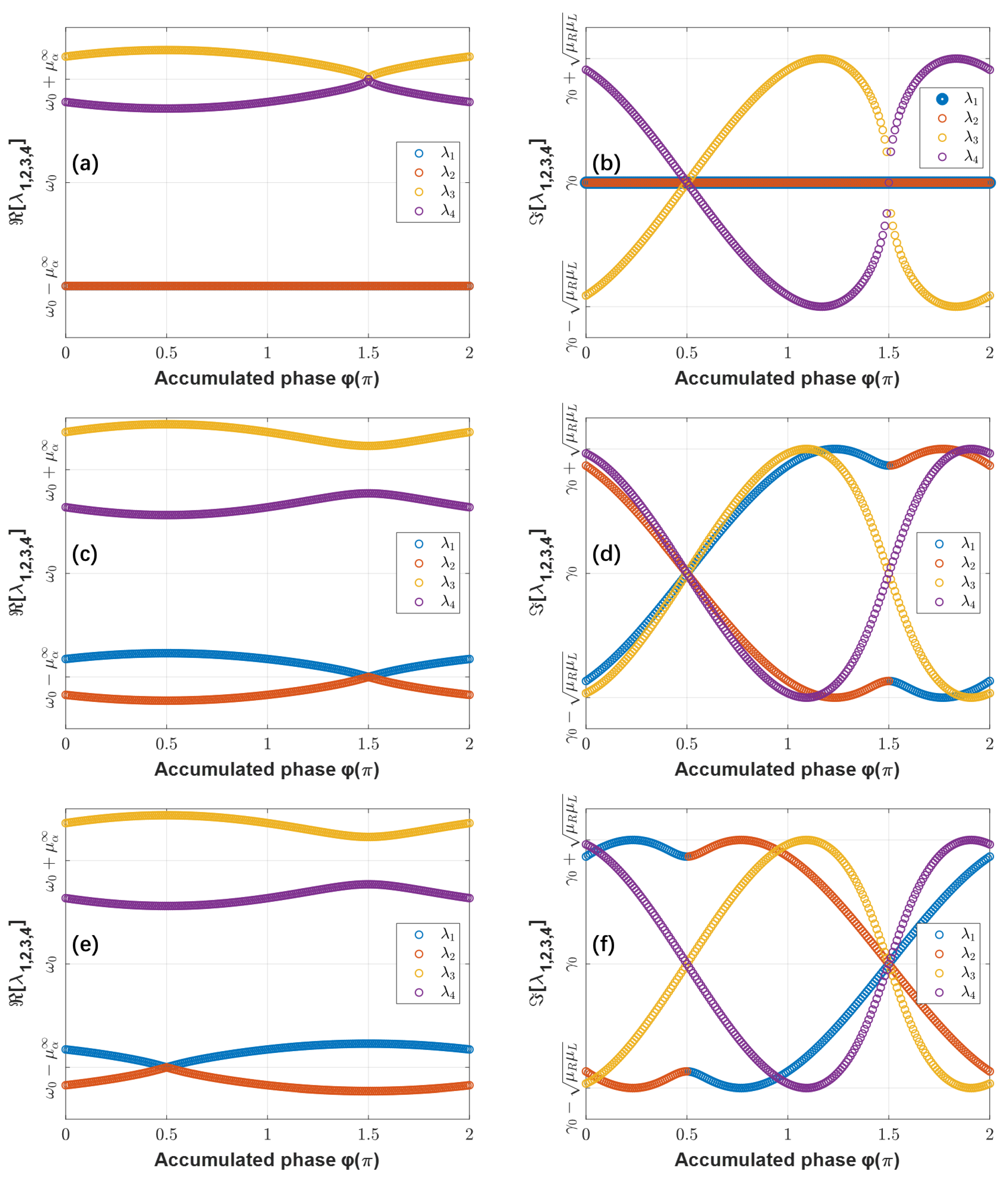
2.1. Eigenvalue Analysis

From Equation (3), we derive the non-Hermitian Hamiltonian of the system as:

$$\widehat{H}=\left[\begin{array}{cccc}{\omega }_0-j{\gamma }_0& {\mu }_a^{\infty }& {\mu }_1^{CW-CCW}& {\mu }_a^{CW}\\ {\mu }_a^{\infty }& {\omega }_0-j{\gamma }_0& {\mu }_a^{CW}& {\mu }_1^{CW-CCW}\\ {\mu }_1^{CW-CCW}& {\mu }_a^{CW}-j{\mu }_R{\mu }_L{e}^{j\phi }& {\omega }_0-j{\gamma }_0& {\mu }_a^{\infty }\\ {\mu }_a^{CW}-j{\mu }_L{\mu }_R{e}^{j\phi }& {\mu }_1^{CW-CCW}& {\mu }_a^{\infty }& {\omega }_0-j{\gamma }_0\end{array}\right]$$

(6)

Considering lossless coupling between units, then the coupling and loss rates are real and positive, and all parameters in this matrix are >0. The eigenvalues of $\widehat{H}$ are given in Equations (7)–(10), with the real parts $\Re \left({\lambda }_{1,2,3,4}\right)$ representing the frequency of the spectral resonances and the imaginary parts $\Im \left({\lambda }_{1,2,3,4}\right)$ their linewidths.

$${\lambda }_1={\omega }_0-j{\gamma }_0-{\mu }_a^{\infty }+\sqrt{{({\mu }_a^{CW}-{\mu }_1^{CW-CCW})}^2-j({\mu }_a^{CW}-{\mu }_1^{CW-CCW}){\mu }_L{\mu }_R{e}^{j\phi }}$$

(7)

$${\lambda }_2={\omega }_0-j{\gamma }_0-{\mu }_a^{\infty }-\sqrt{{({\mu }_a^{CW}-{\mu }_1^{CW-CCW})}^2-j({\mu }_a^{CW}-{\mu }_1^{CW-CCW}){\mu }_L{\mu }_R{e}^{j\phi }}$$

(8)

$${\lambda }_3={\omega }_0-j{\gamma }_0+{\mu }_a^{\infty }+\sqrt{{({\mu }_a^{CW}+{\mu }_1^{CW-CCW})}^2-j({\mu }_a^{CW}+{\mu }_1^{CW-CCW}){\mu }_L{\mu }_R{e}^{j\phi }}$$

(9)

$${\lambda }_4={\omega }_0-j{\gamma }_0+{\mu }_a^{\infty }-\sqrt{{({\mu }_a^{CW}+{\mu }_1^{CW-CCW})}^2-j({\mu }_a^{CW}+{\mu }_1^{CW-CCW}){\mu }_L{\mu }_R{e}^{j\phi }}$$

(10)

Figure 2 illustrates a three-dimensional view for the variation in the eigenvalues with ${\mu }_1^{CW-CCW}$ and $\phi$. We find that there is a PT symmetry property of the system when $\phi =\frac{\pi }{2}$ and $\phi =\frac{3\pi }{2}$.

For an accumulated phase, $\phi =\frac{\pi }{2}$, when ${\mu }_L{\mu }_R>({\mu }_1^{CW-CCW}-{\mu }_a^{CW})>0$, $\Re \left({\lambda }_1\right)=\Re \left({\lambda }_2\right)$ and $\Im \left({\lambda }_1\right)\ne (\Im \left({\lambda }_2\right)$, representing the so-called broken PT symmetry state. For the same accumulated phase, when $({\mu }_1^{CW-CCW}-{\mu }_a^{CW})<0$ or $({\mu }_1^{CW-CCW}-{\mu }_a^{CW})>{\mu }_L{\mu }_R$, then $\Re \left({\lambda }_1\right)\ne \Re \left({\lambda }_2\right)$ and $\Im \left({\lambda }_1\right)=\Im \left({\lambda }_2\right)$, representing the unbroken PT symmetry state, as shown in Figure 3.

Figure 4 shows that, for an accumulated phase, $\phi =\frac{3\pi }{2}$, the relationship between ${\lambda }_1$ and ${\lambda }_2$ is similar to that for $\phi =\frac{\pi }{2}$ for $({\mu }_1^{CW-CCW}+{\mu }_a^{CW})<{\mu }_L{\mu }_R$, $\Re \left({\lambda }_3\right)=\Re \left({\lambda }_4\right)$ and $\Im \left({\lambda }_3\right)\ne \Im \left({\lambda }_4\right)$, i.e., the broken PT symmetry state and for $({\mu }_1^{CW-CCW}+{\mu }_a^{CW})>{\mu }_L{\mu }_R$, $\Re \left({\lambda }_3\right)\ne \Re \left({\lambda }_4\right)$ and $\Im \left({\lambda }_3\right)=\Im \left({\lambda }_4\right)$, i.e., the unbroken PT symmetry state. It should be noted that broken and unbroken PT symmetric states for this system will be difficult to realize in practice because optical modes of different frequencies, propagating in the bus waveguide, will experience different $\phi$.

Figure 5 illustrates how the eigenvalues vary with $\phi$ for different coupling rates, ${\mu }_1^{CW-CCW}$ and ${\mu }_a^{CW}$. When ${\mu }_a^{CW}={\mu }_1^{CW-CCW}$, ${\lambda }_1={\lambda }_2$ and their values are independent of $\phi$, meaning that the resonant system operates at an EP. On the other hand, the eigenvalues ${\lambda }_3$ and ${\lambda }_4$ exhibit a strong dependence on $\phi$.

Even where crosstalk exists between optical modes at the intersection of the ILMR, the system can be made to work at an EP by ensuring ${\mu }_a^{CW}={\mu }_1^{CW-CCW}$. This is good news from a practical perspective because it implies that an ‘ideal’ intersection is not a fundamental requirement for observing EPs in such systems and that some degree of fabrication tolerance can be acceptable.

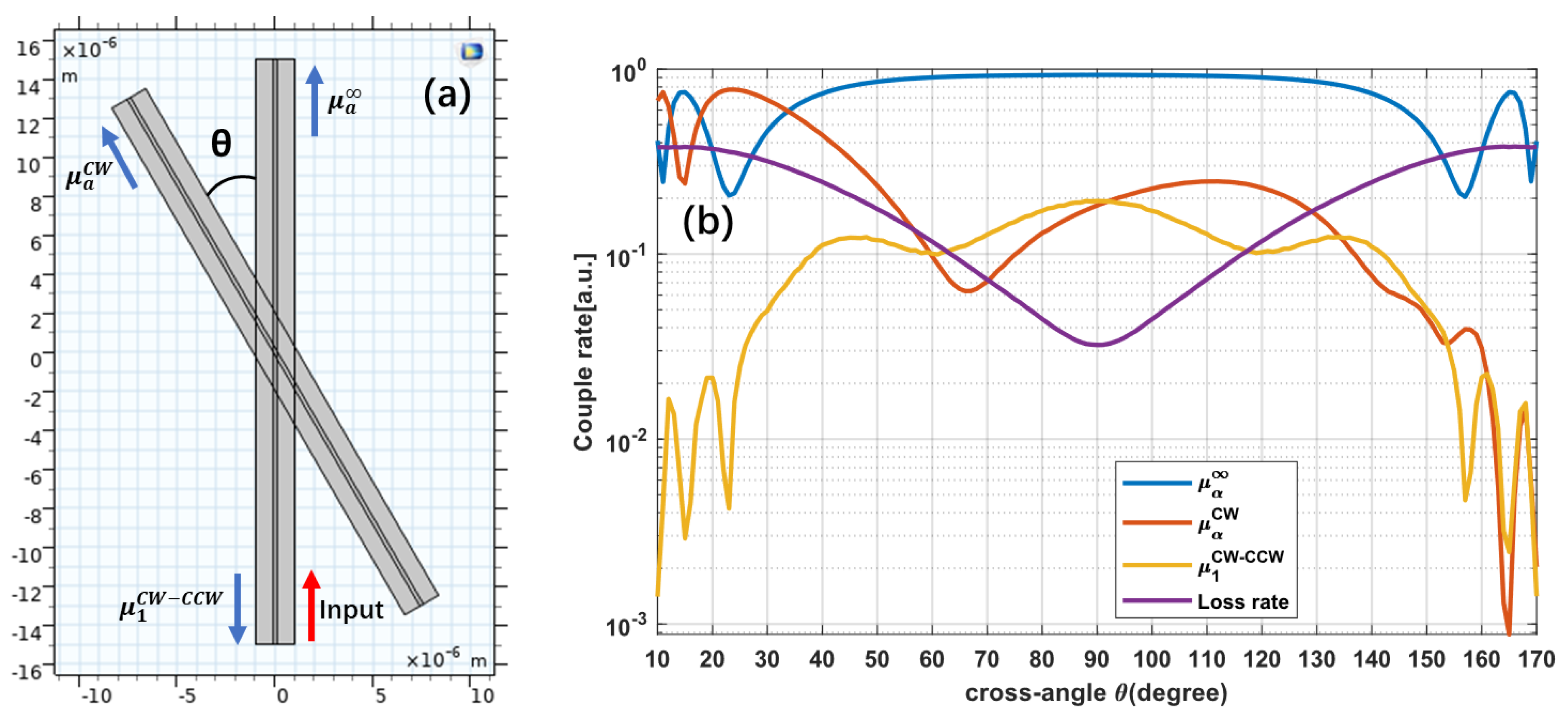
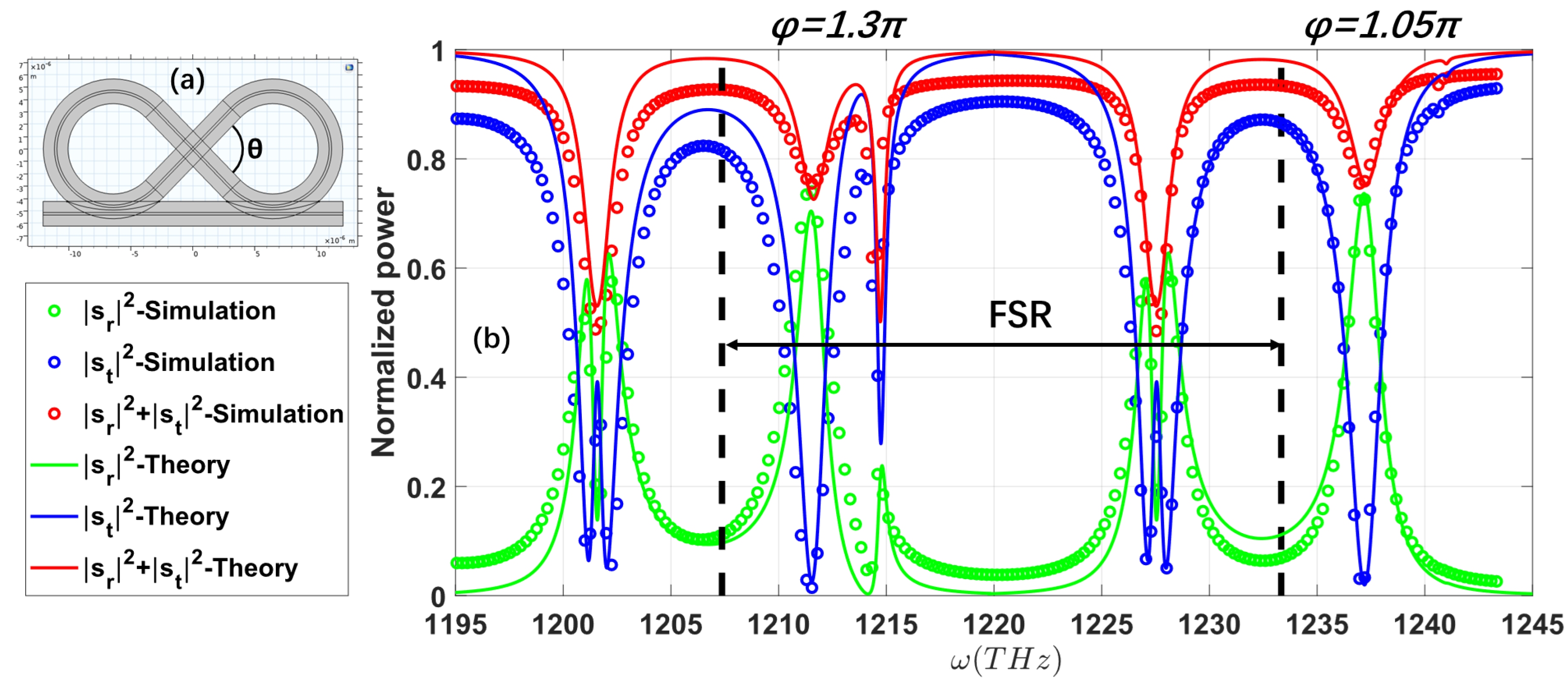
2.2. COMSOL Simulation of Coupling Coefficients between Modes

The coupling rates between resonant modes, as discussed so far for this device, are expected to be a strong function of the crossing angle, $\theta$. For a particular resonance wavelength, e.g., 1550 nm, we can determine the effect of $\theta$ on the individual coupling rates. Assuming the symmetry of the structure is preserved such that ${\mu }_1^{CW-CCW}={\mu }_2^{CW-CCW}$ and ${\mu }_a^{CW}={\mu }_a^{CCW}$, then the coupling rate between resonant modes may be written in terms of the coupling coefficient $\kappa$ and round-trip times $t_1$, $t_2$ [6] as:

$$\mu =\frac{\kappa }{\sqrt{t_1{t}_2}}$$

(11)

Since symmetry implies $t_1=t_2$, the coupling rate is simply proportional to the coupling coefficient and inversely proportional to the resonant unit round trip time. In order to determine the effect of the crossing angle, $\theta$ on coupling (and loss) coefficients, we represented the intersection between resonant modes by a set of crossed straight waveguides using the finite element method (FEM) Multiphysics package in COMSOL, as shown in Figure 6a, the results of which are shown in Figure 6b.

Figure 6b reveals that the strict condition for operation at an EP, i.e., when ${\mu }_a^{CW}={\mu }_1^{CW-CCW}$, is satisfied when the cross angle $\theta \approx {60}^{\circ }$, ${90}^{\circ }$ and ${135}^{\circ }$. We also note that the loss at the intersection is the minimum for $\theta ={92}^{\circ }$.

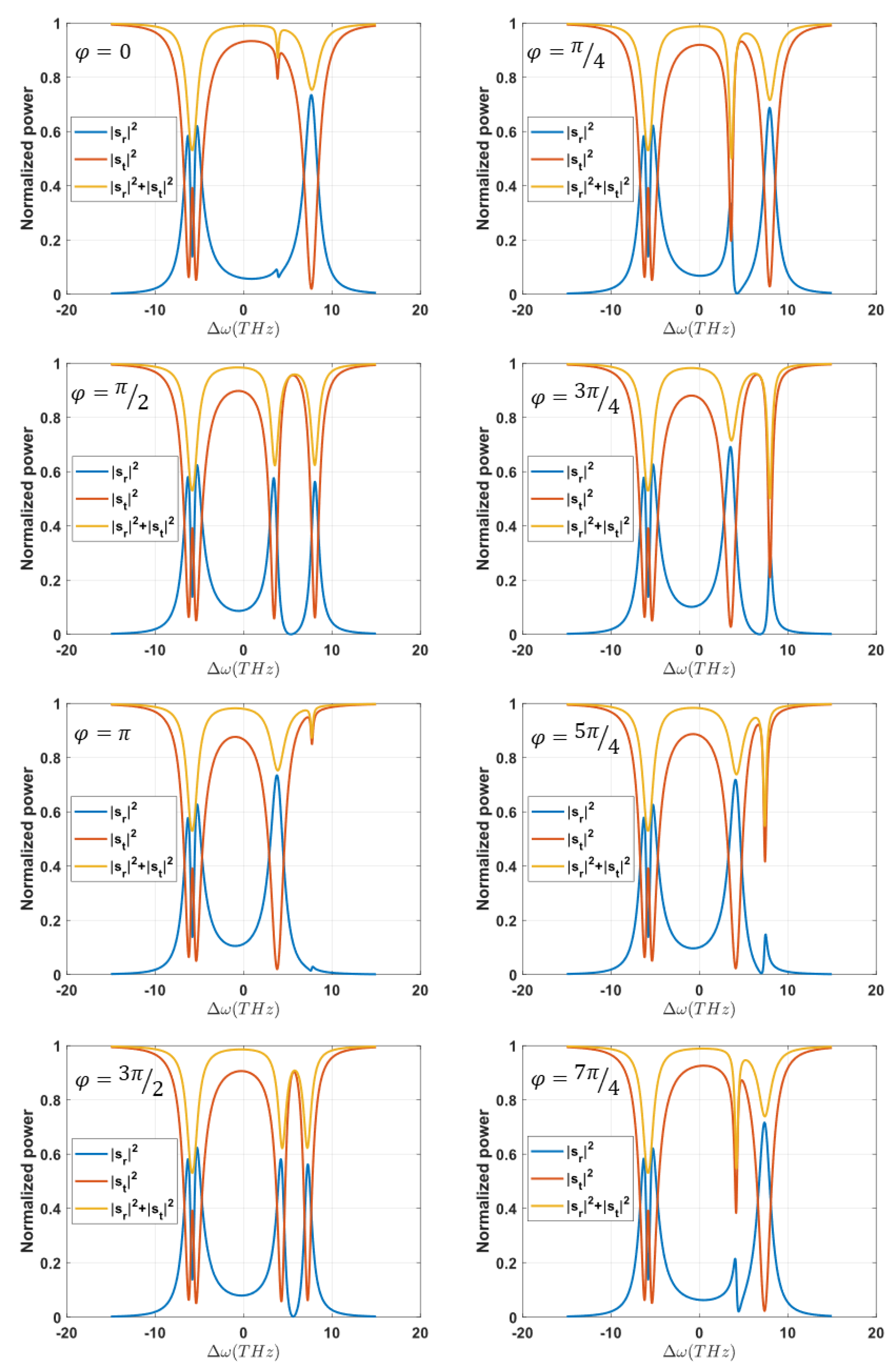
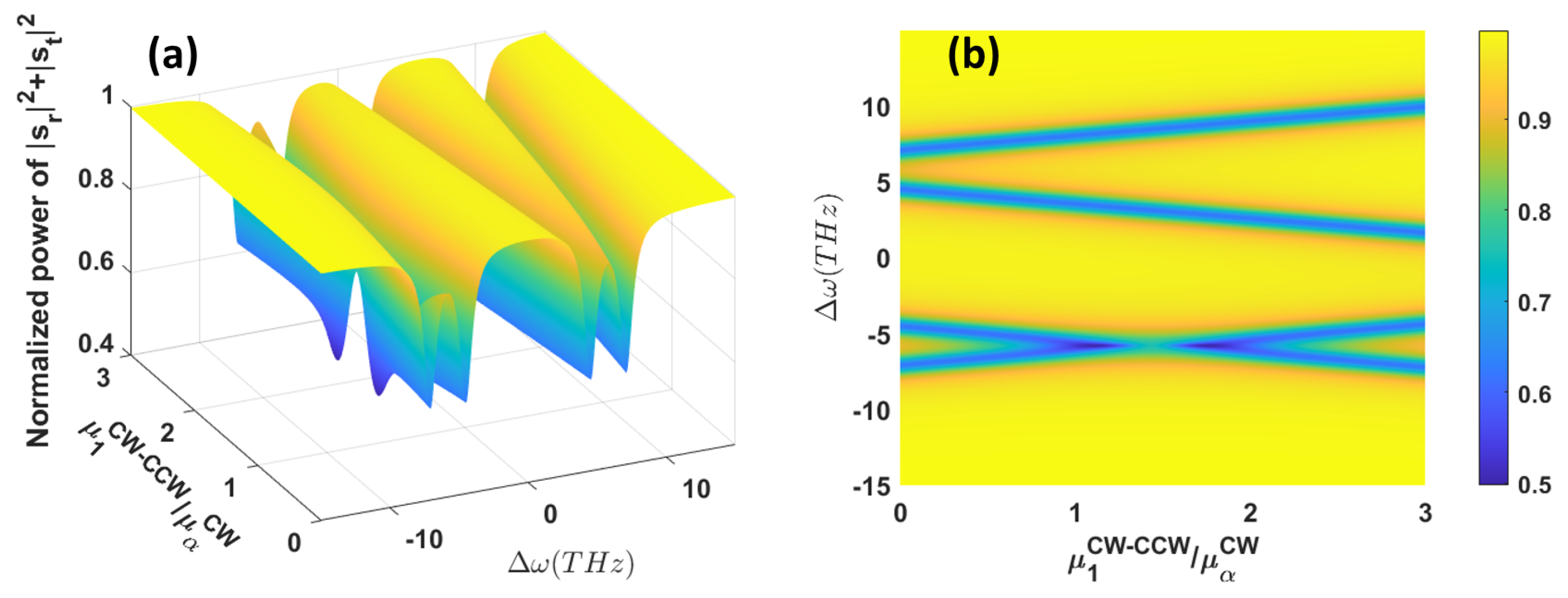
2.3. TCMT-Model-Derived Spectral Resonances

In [16], the transmission and reflection signals are reported to be independent of $\phi$, and so the system apparently always operates at an EP (or on an ES). From the above analysis, we can see that, in reality, this is only the case for ${\lambda }_1$ and ${\lambda }_2$ under the strict condition ${\mu }_a^{CW}={\mu }_1^{CW-CCW}$, which we consider in the subsequent discussion. When the system is in the steady state, the following equations are obtained for resonant propagating modes in either side of the ILMR:

$$\frac{d{a}_i^{CCW}}{dt}=-j\omega a_i^{CCW}$$

(12)

$$\frac{d{a}_i^{CW}}{dt}=-j\omega a_i^{CW}$$

(13)

Table 1. Coupling/loss parameters, derived from Figure 6 used to model the spectral response of the ILMR for low loss operation at an EP.

Parameters	The Coupling/Loss Rates [THz]
${\mu }_a^{\infty }$	5.8037
${\mu }_a^{CW}$	0.9431
${\mu }_1^{CW-CCW}$	0.9431
${{\mu }_L}^2$	0.8152
${{\mu }_R}^2$	0.8152
${\gamma }_0$	0.5421

lists the parameters we employ in modeling the spectral response of the ILMR for low loss operation at an EP.

According to Equations (3)–(5), (11) and (12) and using the parameters in Table 1, as determined from our COMSOL simulations, the spectral response as a function of $\phi$ is shown in Figure 7.

Figure 7 reveals the near-resonance $(\Delta \omega =\omega -{\omega }_0)$ spectral response for the ILMR for ${\lambda }_{1,2}(\Delta \omega <0)$ and ${\lambda }_{3,4}(\Delta \omega >0)$. Although ${\lambda }_1={\lambda }_2$, and the associated (lower-frequency) resonances are independent of $\phi$, we can see that there exists a doublet resonance, which is due to the spectra being formed by the superposition of two optical modes, as revealed by Equations (3) and (4). The sum spectra ${\left|s_t\right|}^2+{\left|s_r\right|}^2$ faithfully reflect the eigenvalues, and in Figure 8, we further illustrate how this varies with the coupling coefficient ${\mu }_1^{CW-CCW}/{\mu }_a^{CW}$ for an accumulated phase, $\phi =\pi /2$, with all other parameters fixed as per Table 1.

Figure 8 shows that, when the coupling rates between the two resonant modes are real and unequal, the eigenvalues of the system exhibit broken and unbroken symmetry states and EPs, as predicted by Equation (6) when $\phi =\pi /2$. This result is traditionally the reserve of active PT symmetric systems, incorporating balanced gain and loss.

The low-frequency spectral peaks are similar to the results of [16], which were also shown to be independent of $\phi$. However, the higher-frequency peaks (i.e., $>{\omega }_0$) are strongly dependent on $\phi$, which is a departure from the general conclusions of [16]. Thus, Using the 4 × 4 matrix model of the ILMR (and devices like it) to include crosstalk between propagating optical fields, and by examining the resulting spectral response on both sides of resonance, it is possible to show that there exists a complexity of peaks, only some of which are independent of $\phi$. In real systems, this might actually represent an expansion of potential applications, e.g., in sensing, filtering and other areas. Indeed, the TCMT modeling approach is generally applicable to other types of resonator, e.g., micro-ring, Fabry–Pérot and photonic crystal cavities, providing the resonant modes and coupling rates between them are determined for the system under study.

3. COMSOL-Simulation-Derived Spectral Resonances

In this section, we extend our use of COMSOL to simulate the complete ILMR structure, as shown in Figure 9a. This consists of two coupled circular waveguide sections, tangential to an input (bus) waveguide. For simplicity, a 2D model based on TE mode is used to avoid superposition of multiple modes, and the width of the waveguide core constrains the system to operate in single mode.

Since we assume lossless coupling between resonant modes in our TCMT model, for closest comparison, we built our COMSOL model around a device geometry that, again, satisfies both minimum coupling loss, i.e., for a cross angle, $\theta ={92}^{\circ }$, from Figure 6, as well as the condition required for operation at an EP, i.e., when ${\mu }_a^{CW}={\mu }_1^{CW-CCW}$. For this value of $\theta$, the total round trip length (perimeter) of our ILMR design is 62.1 µm.

Figure 9b illustrates the results of comparison between the FEM COMSOL simulation and our TCMT model (using the parameters in Table 1) for two neighboring (split) resonances (i.e., over a full FSR). Differences between the TCMT model spectra and those derived from COMSOL simulations are largely due to spectral dependencies of the accumulated phase, $\phi$, and the parameters in Table 1, which were obtained for a fixed angular frequency of 1215.2 THz (1550 nm). Agreement is therefore expected to diverge as the spectral range increases, so we have necessarily adjusted $\phi$ to account for this, finding excellent agreement around the lower-frequency resonance position when $\phi \sim 5\pi /4$ and for the next, higher-frequency resonance, by using a slightly lower value, $\phi \sim \pi$.

4. Conclusions

In this paper, the recently described ILMR is considered as four mutually coupled resonant modes, with cw and ccw propagating optical modes that interact via crosstalk. The eigenvalues and associated transmission and reflection spectra are determined from a 4 × 4 matrix Hamiltonian using TCMT. The specific conditions required for the system to operate at an EP are determined as ${\mu }_a^{CW}={\mu }_{\mathbf{1}}^{CW-CCW}$. The system is also simulated using COMSOL, which provides the key design parameters for effective operation at an EP for wavelengths near 1550 nm. The spectra derived from this simulation for an ILMR with a crossing angle $\theta ={92}^{\circ }$ (operating at an EP with minimal loss) are in good agreement with those derived from our TCMT model. Both simulation and TCMT modeling show that the ILMR has a complex resonance spectrum with ‘split’ peaks either side of the mode resonance $({\omega }_0\pm \omega )$ condition. The lower-frequency spectral peaks $(\omega <{\omega }_0)$ are found to be rather independent of the accumulated phase, $\phi$, in good agreement generally with the model proposed in [16]. However, we find that the higher-frequency peaks $(\omega >{\omega }_0)$ exhibit a strong dependence on $\phi$. We also demonstrate that our TCMT model agrees well with FEM COMSOL simulation of such devices over a full free spectral range (with necessary adjustment of the accumulated phase). The rich spectral form for this and similar devices, along with the type of modeling we have described, can aid the design of practical, non-Hermitian nanophotonic integrated circuits for a whole host of exotic applications, which are only beginning to come to light as this new field emerges.

References

1. Haus, H.; Huang, W. Coupled-mode theory. Proc. IEEE 1991, 79, 1505–1518. [Google Scholar] [CrossRef]
2. Wang, T. Generalized temporal coupled-mode theory for a P T-symmetric optical resonator and Fano resonance in a P T-symmetric photonic heterostructure. Opt. Express 2022, 30, 37980–37992. [Google Scholar] [CrossRef]
3. Zhang, B.; Chen, N.; Lu, X.; Hu, Y.; Yang, Z.; Zhang, X.; Xu, J. Bandwidth Tunable Optical Bandpass Filter Based on Parity-Time Symmetry. Micromachines 2022, 13, 89. [Google Scholar] [CrossRef] [PubMed]
4. Lu, X.; Chen, N.; Zhang, B.; Yang, H.; Chen, Y.; Zhang, X.; Xu, J. Parity-Time Symmetry Enabled Band-Pass Filter Featuring High Bandwidth-Tunable Contrast Ratio. Photonics 2022, 9, 380. [Google Scholar] [CrossRef]
5. Fan, S. 12—Photonic crystal theory: Temporal coupled-mode formalism. In Optical Fiber Telecommunications V A, 5th ed.; Kaminow, I.P., Li, T., Willner, A.E., Eds.; Optics and Photonics; Academic Press: Burlington, MA, USA, 2008; pp. 431–454. [Google Scholar] [CrossRef]
6. Van, V. Optical Microring Resonators: Theory, Techniques, and Applications; CRC Press: Boca Raton, FL, USA, 2016. [Google Scholar] [CrossRef]
7. Behunin, R.O.; Otterstrom, N.T.; Rakich, P.T.; Gundavarapu, S.; Blumenthal, D.J. Fundamental noise dynamics in cascaded-order Brillouin lasers. Phys. Rev. A 2018, 98, 023832. [Google Scholar] [CrossRef]
8. Hu, Y.; Yu, M.; Zhu, D.; Sinclair, N.; Shams-Ansari, A.; Shao, L.; Holzgrafe, J.; Puma, E.; Zhang, M.; Lončar, M. On-chip electro-optic frequency shifters and beam splitters. Nature 2021, 599, 587–593. [Google Scholar] [CrossRef] [PubMed]
9. Rüter, C.E.; Makris, K.G.; El-Ganainy, R.; Christodoulides, D.N.; Segev, M.; Kip, D. Observation of parity–time symmetry in optics. Nat. Phys. 2010, 6, 192–195. [Google Scholar] [CrossRef]
10. Peng, B.; Özdemir, Ş.K.; Lei, F.; Monifi, F.; Gianfreda, M.; Long, G.L.; Fan, S.; Nori, F.; Bender, C.M.; Yang, L. Parity–time-symmetric whispering-gallery microcavities. Nat. Phys. 2014, 10, 394–398. [Google Scholar] [CrossRef]
11. Joglekar, Y.N.; Harter, A.K. Passive parity-time-symmetry-breaking transitions without exceptional points in dissipative photonic systems [Invited]. Photonics Res. 2018, 6, A51–A57. [Google Scholar] [CrossRef]
12. Ma, J.; Wen, J.; Ding, S.; Li, S.; Hu, Y.; Jiang, X.; Jiang, L.; Xiao, M. Chip-Based Optical Isolator and Nonreciprocal Parity-Time Symmetry Induced by Stimulated Brillouin Scattering. Laser Photonics Rev. 2020, 14, 1900278. [Google Scholar] [CrossRef]
13. Calabrese, A.; Ramiro-Manzano, F.; Price, H.M.; Biasi, S.; Bernard, M.; Ghulinyan, M.; Carusotto, I.; Pavesi, L. Unidirectional reflection from an integrated “taiji” microresonator. Photonics Res. 2020, 8, 1333–1341. [Google Scholar] [CrossRef]
14. Biasi, S.; Franchi, R.; Mione, F.; Pavesi, L. Interferometric method to estimate the eigenvalues of a non-Hermitian two-level optical system. Photonics Res. 2022, 10, 1134–1145. [Google Scholar] [CrossRef]
15. Zhong, Q.; Ren, J.; Khajavikhan, M.; Christodoulides, D.; Özdemir, Ş.K.; El-Ganainy, R. Sensing with Exceptional Surfaces in Order to Combine Sensitivity with Robustness. Phys. Rev. Lett. 2019, 122, 153902. [Google Scholar] [CrossRef]
16. Franchi, R.; Biasi, S.; Piciocchi, D.; Pavesi, L. The infinity-loop microresonator: A new integrated photonic structure working on an exceptional surface. APL Photonics 2023, 8, 056111. [Google Scholar] [CrossRef]
17. Dingel, B.B.; Nacpil, J.C. Multifunctional tunable band-limited optical Coupled-Ring Reflector (CRR) device using criss-crossing directional coupler. In Proceedings of the 2021 IEEE Region 10 Symposium (TENSYMP), Jeju, Republic of Korea, 23–25 August 2021; pp. 1–5. [Google Scholar] [CrossRef]
Figure 1. Infinity loop micro-resonator (ILMR) structure (a) without and (b) with counter propagating optical pathways within units, a 1 and a 2 , which are coupled at the intersection, modified after [16].
Symmetry 16 00430 g001
Figure 2. (a) Real and (b) imaginary components of the H ^ eigenvalues as a function of the coupling rate, μ 1 C W C C W , and accumulated phase, φ , when μ a C W < μ L μ R .
Symmetry 16 00430 g002
Figure 3. (a) Real and (b) imaginary components of the H ^ eigenvalues as a function of the coupling rate, μ 1 C W C C W , for an accumulated phase, φ = π 2 between ILMR bus-to-loop coupling points.
Symmetry 16 00430 g003
Figure 4. (a,c) Real and (b,d) imaginary components of the H ^ eigenvalues as a function of the coupling rate, μ 1 C W C C W , for accumulated phase φ = 3 π 2 between ILMR bus-to-loop coupling points. The upper (a,b) and lower (c,d) panels are for the case when μ a C W > μ L μ R and μ a C W < μ L μ R .
Symmetry 16 00430 g004
Figure 5. (a,c,e) Real and (b,d,f) imaginary components of the H ^ eigenvalues as a function of φ . The upper (a,b), middle (c,d) and lower (e,f) panels represent the cases; μ 1 C W C C W = μ a C W , μ 1 C W C C W < μ a C W and μ 1 C W C C W > μ a C W , respectively.
Symmetry 16 00430 g005
Figure 6. (a) Model of the ILMR crossed-waveguide section and (b) corresponding COMSOL simulation of the individual coupling and loss coefficients as a function of the ILMR crossing angle, θ , at 1550 nm.
Symmetry 16 00430 g006
Figure 7. Transmission and reflection spectra, s t 2 and s r 2 and s t 2 + s r 2 , for different values of accumulated phase, φ .
Symmetry 16 00430 g007
Figure 8. 3D plots of (a) spectral response and (b) peak positions for s t 2 + s r 2 as a function of the coupling coefficient μ 1 C W C C W / μ a C W for an accumulated phase, φ = π / 2 .
Symmetry 16 00430 g008
Figure 9. (a) COMSOL ILMR model structure with crossing angle, θ = 92 and total round-trip length (perimeter) = 62.1 µm and (b) corresponding spectral response (COMSOL (points) and TCMT model (lines)). The accumulated phase, φ , is necessarily adjusted in our TCMT model (from 5 π / 4 to π ) to account for the wide frequency range (>1 FSR, as indicated by the black dashed lines) of the COMSOL simulation.
Symmetry 16 00430 g009