1. Introduction and the Model
Optical solitons are a broad class of self-trapped states maintained by the interplay of nonlinearity and dispersion or diffraction in diverse photonic media [
1,
2]. In addition to that, dissipative optical solitons are supported by the equilibrium of loss and gain or pump, which is concomitant to the nonlinearity–dispersion/diffraction balance [
3,
4]. Dissipative solitons have been studied in detail, theoretically and experimentally, in active setups, with the loss compensated by local gain (essentially provided by lasing) being modeled by one- and two-dimensional (1D and 2D) equations of the complex Ginzburg–Landau (CGL) type [
5,
6].
In passive nonlinear optical cavities, the losses are balanced by the pump field supplied by external laser beams, with the appropriate models provided by the Lugiato–Lefever (LL) equations [
7]. This setting was also studied in the 1D and 2D forms [
8,
9,
10,
11]. Widely applied in nonlinear optics, equations of the LL type play a crucial role in understanding fundamental phenomena such as the modulation instability (MI) and pattern formation in dissipative environments [
8,
9,
10,
11,
12,
13,
14,
15,
16,
17,
18,
19,
20,
21,
22,
23,
24]. The relevance of these models extends to the exploration of complex dynamics of various nonlinear photonic modes, with tremendously important applications being the generation of Kerr solitons and frequency combs in passive cavities [
12,
13,
14,
15,
16,
17,
18,
19,
20,
21,
22,
23,
24], as well as the generation of terahertz radiation [
25]. In addition to rectilinear cavity resonators, circular ones can be used too [
26]. In many cases, they operate in the whispering gallery regime [
27,
28,
29,
30,
31,
32].
In most cases, solutions of the one- and two-dimensional LL equations are looked for under the action of a spatially uniform pump, which approximately corresponds to the usual experimental setup. However, the use of localized (focused) pump beams is possible too, which makes it relevant to consider LL equations with the respective shape of the pump terms. In fact, truly localized optical modes in the cavities can be created only in this case; otherwise, the uniform pump supports the nonzero background of the optical field. In particular, exact analytical solutions of the LL equations with the 1D pump represented by the delta function and approximate solutions maintained by the 2D pump in the form of a Gaussian were reported in Ref. [
33]. In Ref. [
26], the LL equation for the ring resonator with localized pump and loss terms produced nonlinear resonances leading to the multistability of nonlinear modes and coexisting solitons that are associated with spectrally distinct frequency combs.
Furthermore, solutions for fully localized robust pixels with zero background were produced by the 2D LL equation, thereby incorporating the spatially uniform pump, self-focusing or defocusing cubic nonlinearity, and a tight confining harmonic oscillator potential [
34]. Additionally, this model with a vorticity-carrying pump gives rise to stable vortex pixels. In particular, in the case of the self-defocusing sign of the nonlinear term, the pixels with zero vorticity and ones with vorticity
were predicted analytically by means of the Thomas–Fermi (TF) approximation.
In this work, we introduce the 2D LL equation for a complex amplitude field
of the light field with cubic or cubic–quintic nonlinearity:
and a confined pump beam represented by factor
. Here,
i is the imaginary unit,
is the loss parameter,
and
correspond, respectively, to the self-focusing and defocusing Kerr (cubic) nonlinearity,
or
represent the self-defocusing or focusing quintic nonlinearity (which often occurs in optical media [
35,
36,
37] in addition to the cubic term), parameter
defines the cavity mismatch—which is
(the coefficient multiplying the linear term
) in terms of the linearized LL equation—and
written in terms of polar coordinates
, which corresponds to the confined pump beam with real amplitude
, radial width
W, and integer vorticity
. Vortex beams, shaped by the passage of the usual laser beam through an appropriate phase mask, are available in the experiment [
37].
Equation (
1) is written in the scaled form. All figures (
Figure 1,
Figure 2,
Figure 3,
Figure 4,
Figure 5,
Figure 6,
Figure 7,
Figure 8,
Figure 9,
Figure 10,
Figure 11,
Figure 12 and
Figure 13) are plotted below in the same notation. In physical units,
and
normally correspond to ∼50 m and
ps, respectively. Then, the typical width
, considered below, corresponds to the pump beam with diameter ∼100 m, which is an experimentally relevant value. Accordingly, the characteristic evolution time in simulations presented below,
100, corresponds to the time
ns.
Stationary solutions of Equation (
1) are characterized by values of the total power (alias norm):
and the angular momentum is characterized as
(with ∗ standing for the complex conjugate), even if the power and angular momentum are not dynamical invariants of the dissipative Equation (
1). In the case of the axisymmetric solutions with vorticity
S, i.e.,
[
38,
39,
40], the expressions for the power and angular momentum are simplified:
Our objective is to construct
stable ring-shaped vortex solitons (representing vortex pixels in terms of plausible applications) as localized solutions of Equation (
1) with the same
S as in the pump term (
2). The stability is a challenging problem, as it is well known from the work with models based on the nonlinear Schrödinger and CGL equations that (in the absence of a tight confining potential) vortex ring solitons are normally vulnerable to splitting instability. In the case of a narrow ring shape, the splitting instability may be considered as quasi-one-dimensional MI of the ring against azimuthal perturbations, which break its axial symmetry [
2,
40]. The azimuthal MI is driven by the self-focusing nonlinearity and inhibited by the self-defocusing.
To produce stationary solutions for the vortex solitons in an approximate analytical form (parallel to the numerical solution), we employ a variational approximation (VA). Our results identify regions of the existence and stability of the vortex solitons with
in the space of parameters of Equations (
1) and (
2) (in particular, in the plane of
) for both signs of the cubic nonlinearity,
, while the mismatch parameter is fixed to be
by the dint of scaling. The stability areas are vast, provided that the loss coefficient
is, roughly speaking, not too small. A majority of the results are produced for the pure cubic model, with
, but the effect of the quintic term, with
, is considered too. Quite surprisingly, a stability area for the vortices with
was found even in the case of
, when both the cubic and quintic terms were self-focusing, which usually implies a strong propensity to the azimuthal instability of the vortex rings [
40].
The rest of the paper is structured as follows. The analytical approach, based on the appropriate VA, is presented in
Section 2. An asymptotic expression for the tail of the vortex solitons, decaying at
, is found too in that section. Systematically produced numerical results for the shape and stability of the vortex solitons are collected (and compared to the VA predictions) in
Section 3. The paper is concluded by
Section 4.
3. Numerical Results
Simulations of Equation (
1) were conducted by means of the split-step pseudospectral algorithm. The solution procedure started from the zero input and was running until convergence to an apparently stable stationary profile (if this outcome of the evolution was possible). This profile was then compared to its VA counterpart, which was produced by a numerical solution of Equations (
18) and (
19) with the same values of parameters
,
,
g,
,
W, and
S (see Equation (
2)). The results are presented below by varying, severally, loss
, vorticity
S, the pump’s width
W, strength
, and, eventually, the quintic coefficient
g. The findings were eventually summarized in the form of stability charts plotted in
Figure 12.
3.1. Variation in the Loss Parameter
In
Figure 2a, we display the cross-section (drawn through
) of the variational and numerical solutions for the stable vortex solitons obtained with
,
, and
, while the other parameters were fixed as
(the self-focusing cubic nonlinearity),
,
,
, and
. The accuracy of the VA-predicted solutions presented in
Figure 2a are characterized by the relative power differences from their numerically found counterparts, which resulted in
,
, and
for
respectively. Thus, the VA accuracy improves with the increase in
.
Similar results for the self-defocusing nonlinearity,
, are presented in
Figure 2b, which shows an essentially larger discrepancy between the VA and numerical solutions,
viz.,
,
, and
for the same set (
28) of values of the loss parameter, with the other coefficients being the same as in
Figure 2a. The larger discrepancy is explained by the fact that localized (bright soliton) modes are not naturally maintained by the self-defocusing; hence, the ansatz (
14), which is natural for the self-trapped solitons in the case of self-focusing, is not accurate enough for
. In the same vein, it is natural that, in the latter case, the discrepancy is more salient for stronger nonlinearity, i.e., smaller
, which makes the respective amplitude higher.
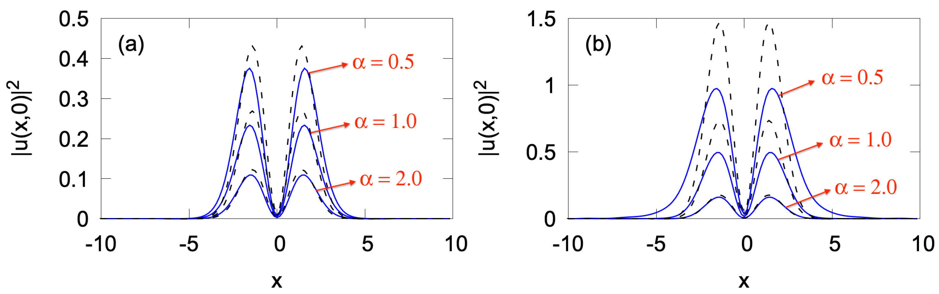
Figure 2.
The comparison between cross-sections (drawn through
) of the VA solutions and their numerically found counterparts (dashed black and solid blue lines, respectively) for different values of the loss parameter
in Equation (
1) taken from set (
28). Panels (
a,
b) pertain to the self-focusing (
) and defocusing (
) signs of cubic nonlinearity, respectively. The other parameters in Equations (
1) and (
2) are fixed as
,
,
,
, and
.
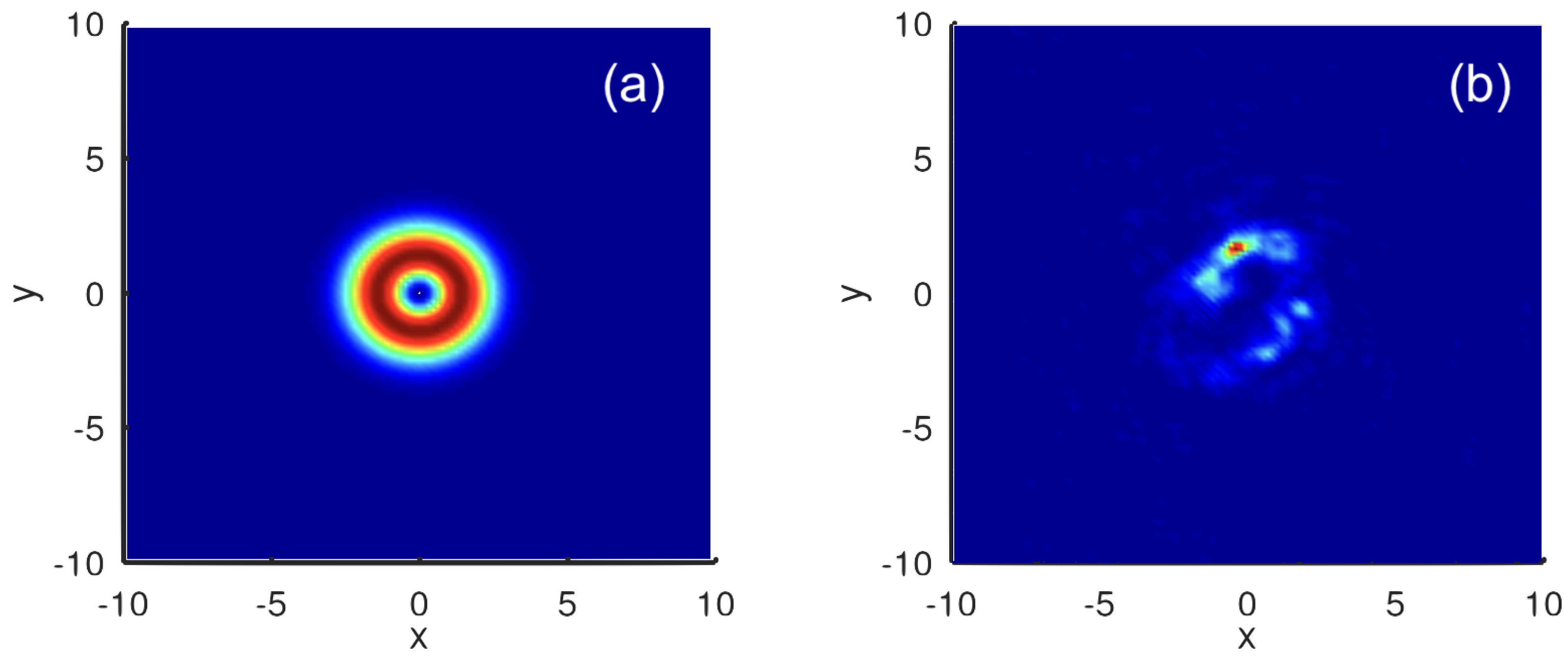
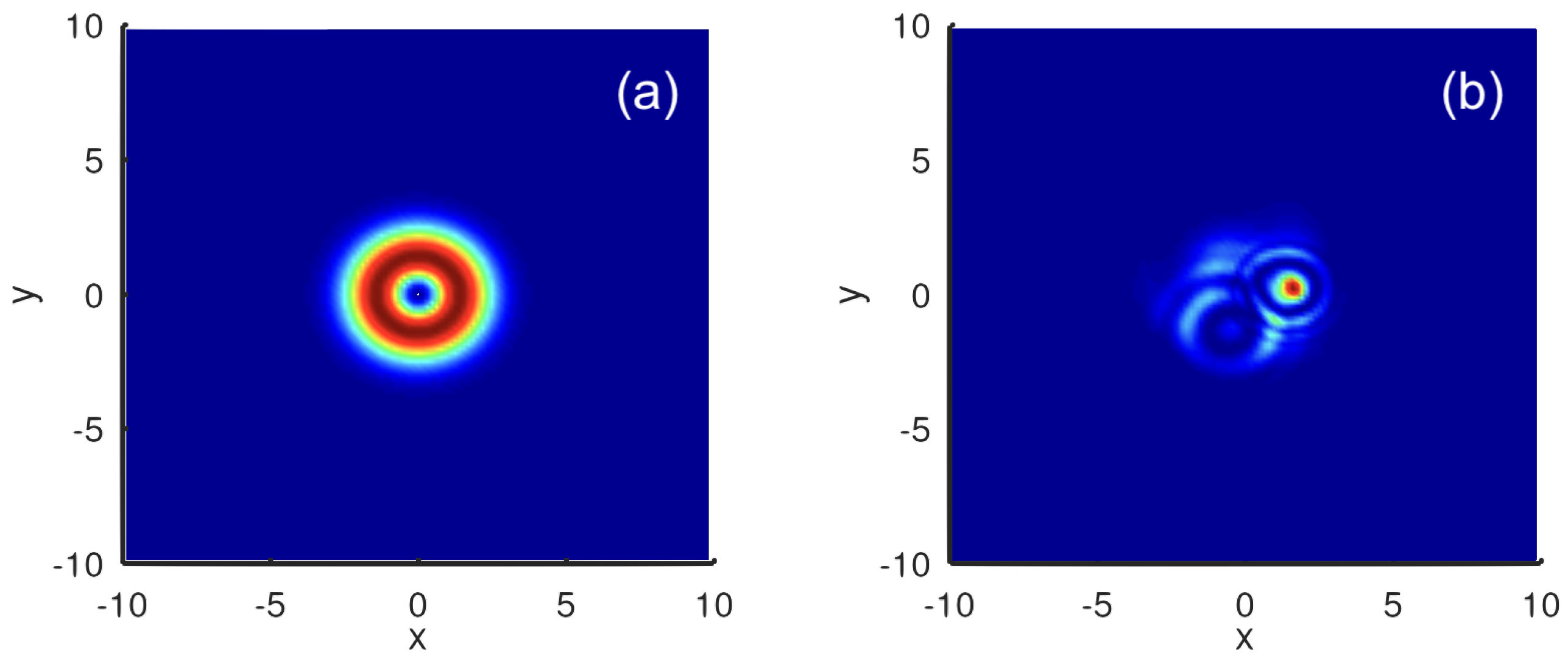
There is a critical value of
below which the vortex solitons are unstable. As an example,
Figure 3 shows the VA-predicted and numerically produced solutions for
and
(self-focusing nonlinearity). The observed picture may be understood as a result of the above-mentioned azimuthal MI, which breaks the axial symmetry of the vortex soliton. More examples of the instability of this type are displayed below. For the values of the other parameters fixed as in
Figure 3, the instability boundary was
. The stabilizing effect of the loss at
is a natural feature. On the other hand, the increase in
led to a decrease in the soliton’s amplitude, as seen in
Figure 2.
Figure 3.
Profiles of
produced by VA (
a) and numerical solution at
(
b) in the case of self-focusing (
) for
. Other parameter are the same as in
Figure 2a.
Figure 3.
Profiles of
produced by VA (
a) and numerical solution at
(
b) in the case of self-focusing (
) for
. Other parameter are the same as in
Figure 2a.
In the case of self-defocusing (), all the numerically found vortex modes were stable, at least, at , although the discrepancy in the values of the power between these solutions and their VA counterparts was very large at small , thereby exceeding at . As mentioned above, the growing discrepancy is explained by the increase in the soliton’s amplitude with the decrease in . At still smaller values of , the relaxation of the evolving numerical solution toward the stationary state is very slow, which makes it difficult to identify the stability.
3.2. Variation in the Pump’s Vorticity S
To analyze the effects of the winding number (vorticity)
S, we fixed
(the pure cubic nonlinearity) and set
,
,
in Equations (
1) and (
2). In the self-focusing case (
), the numerically produced solutions were stable for
and 2 and unstable for
. In the former case, the power differences between the VA and numerical solutions were
and
for
and 2, respectively, i.e., the VA remains a relatively accurate approximation in this case.
In the self-defocusing case (), considering the same values of the other parameters as used above, the numerical solution produced stable vortex solitons at least until . For the same reason as mentioned above, the accuracy of the VA was much lower for than for the self-focusing case (), with the respective discrepancies in the power values being , , , , and for , 2, 3, 4, and 5, respectively.
For the cogent verification of the stability of the localized vortices in the case of self-defocusing, we also checked it for smallest value of the loss parameter considered in this work,
viz.,
, again for
, 2, 3, 4, and 5, and the above-mentioned values of the other coefficients, i.e.,
and
. Naturally, the discrepancy between the VA and numerical findings was still higher in this case, being
,
,
,
, and
for
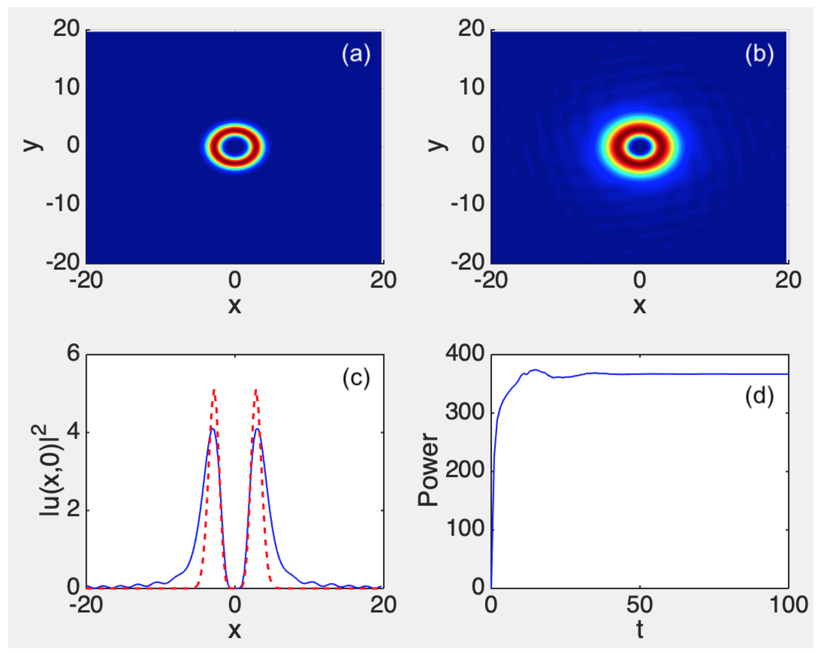
, 2, 3, 4, and 5, respectively. The result is illustrated in
Figure 4 for a relatively large vorticity,
. In particular, the pattern of
and the corresponding cross-section, displayed in
Figure 4b,c, respectively, exhibit the established vortex structure and background “garbage” produced by the evolution.
Figure 4.
(
a) The VA-predicted pattern and (
b) the corresponding result of the direct simulation of Equation (
1) with
and
(cubic self-defocusing) at
, initiated by the zero input at
for
,
,
, and vorticity
in the pump term (
2). (
c) The respective cross-sections drawn through
. (
d) The evolution of the total power
P (see Equation (
3) of the numerical solution in the course of the simulation.
3.3. Variation in the Pump’s Width W
To address the effects of the variation in parameter
W in Equation (
2), we fixed
,
,
, and
. In
Figure 5a, the power of the VA-predicted and numerically found stable vortex soliton solutions are plotted as a function of
W for both the self-focusing and defocusing cases, i.e.,
and
, respectively. In the former case, the azimuthal MI set in at
; see an example in
Figure 5b for
.
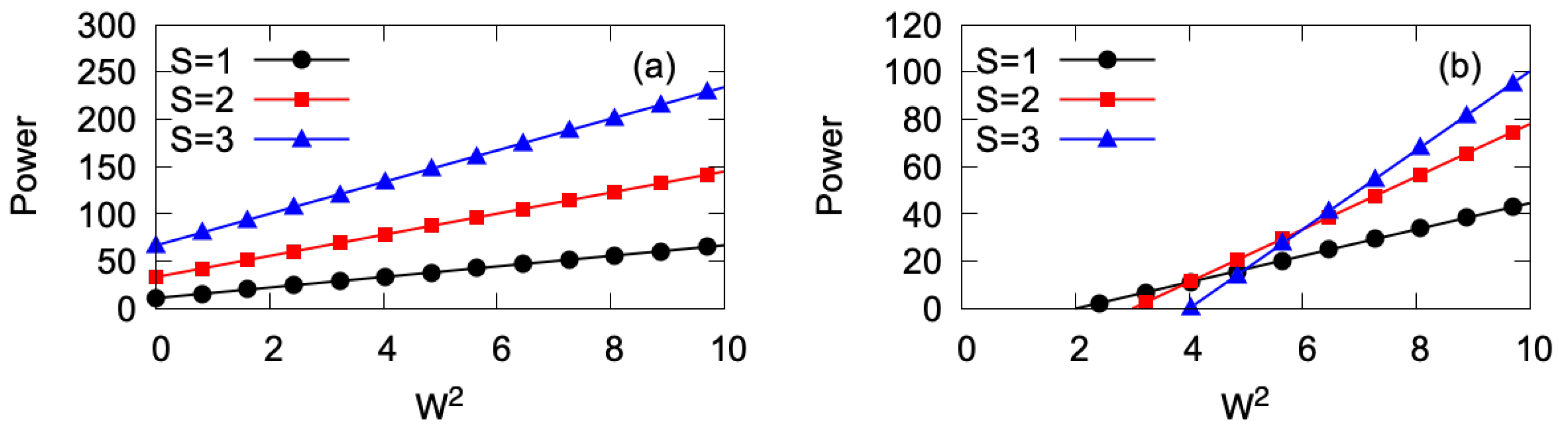
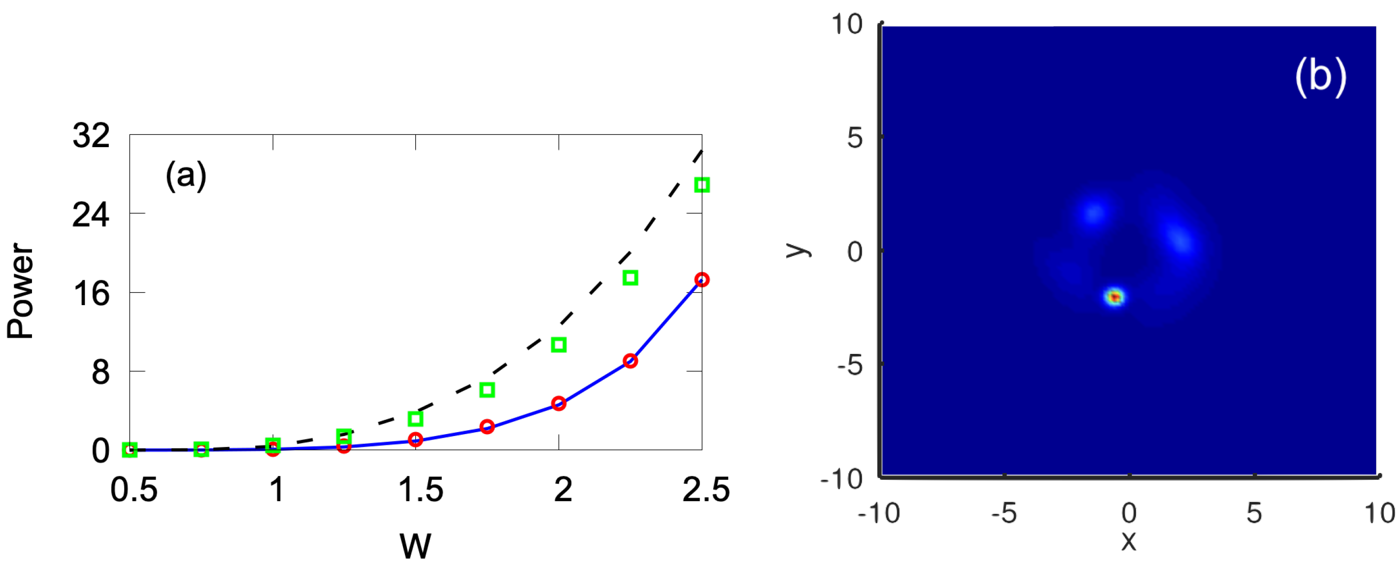
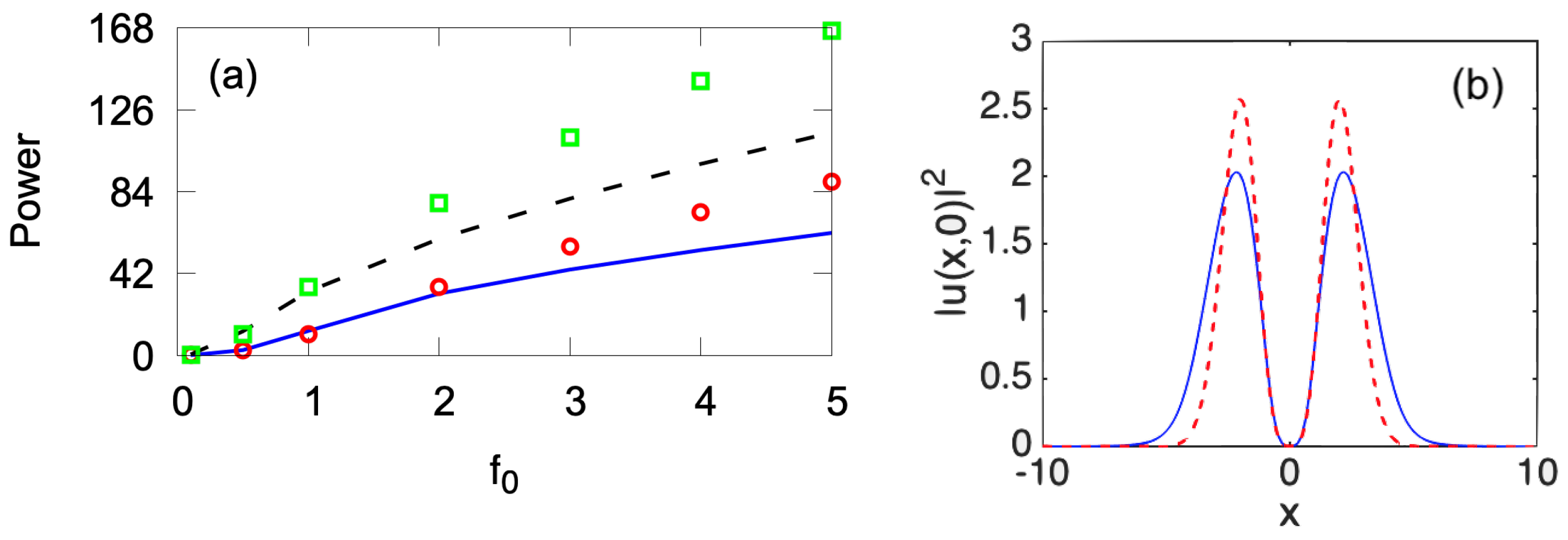
Figure 5.
(a) The power of the VA-predicted vortex soliton solutions (solid blue and dashed black lines pertaining to the self-focusing, , and self-defocusing, , cubic nonlinearitry, respectively) and their numerically found counterparts (red circles and green squares pertaining to the self-focusing and self-defocusing nonlinearitry, respectively) vs. the pump’s width W. Other parameters are , , , and . (b) The profile produced, at , by the numerically generated unstable solution in the case of the self-focusing, , with .
In the self-focusing case, , the azimuthal MI for the solitons with higher vorticities, , 3, 4, or 5, set in at , , , and , respectively. In the self-defocusing case, no existence/stability boundary was found for the vortex modes with , , and (at least up to ). At higher values of the vorticity, the localized vortices do not exist; in the defocusing case, they exist at and for and , respectively.
3.4. Variation in the Pump’s Strength
The effects of the variation in
are reported here, where we fixed the other parameters as
,
, and
. In the case of the cubic self-focusing,
, the vortex soliton with
was subject to an MI at
. As a typical example, in
Figure 6, we display the VA-predicted solution alongside the result of the numerical simulations for
. For higher vorticities,
, 3, 4, and 5, the azimuthal instability set in at
,
,
, and
, respectively. Naturally, the narrow vortex rings with large values of
S are much more vulnerable to the quasi-one-dimensional azimuthal MI.
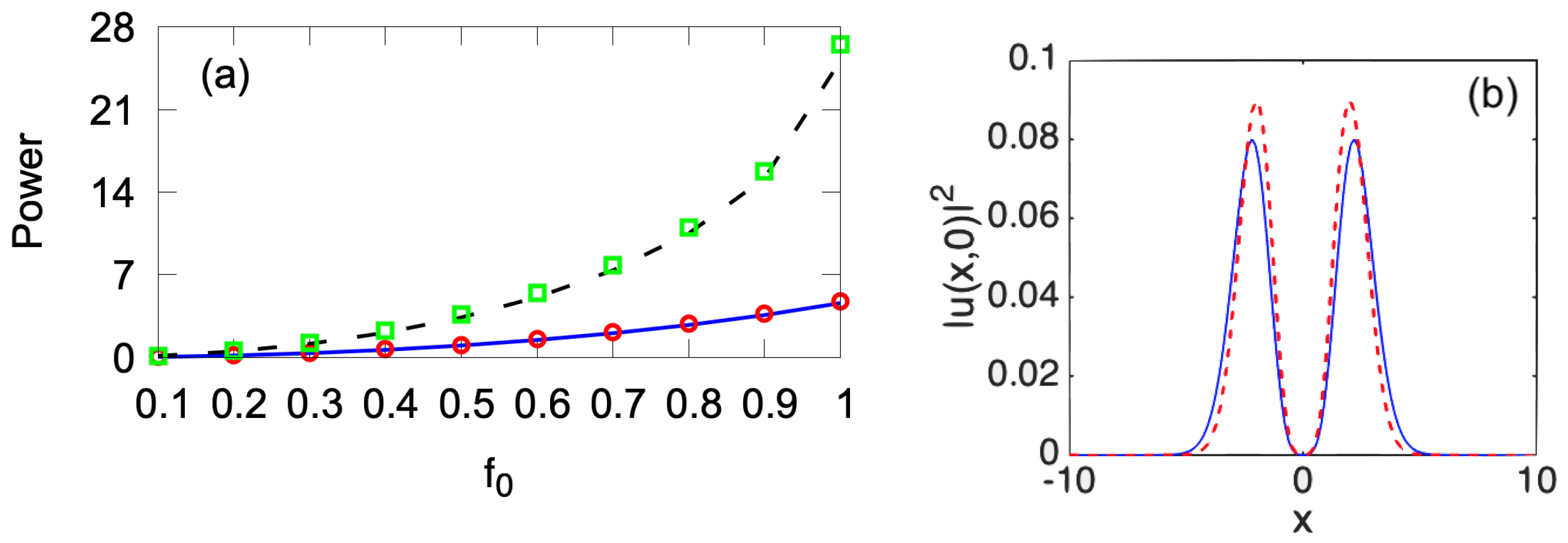
The power of the vortex solitons with
and 2, as produced by the VA and numerical solution, is plotted vs. the pump amplitude
in
Figure 7a. As an example,
Figure 7b showcases an example of the cross-section profile of the vortex soliton with
, thus demonstrating the reliability of the VA prediction. In the range of
, the highest relative difference in the power between the numerical and variational solutions cases was
and
for
and
, respectively.
Figure 6.
(
a) The VA-predicted profile of
in the self-focusing case, with parameters
,
,
,
,
, and
. (
b) The unstable solution, produced at
, by the simulations of Equation (
1) for the same parameters.
Figure 6.
(
a) The VA-predicted profile of
in the self-focusing case, with parameters
,
,
,
,
, and
. (
b) The unstable solution, produced at
, by the simulations of Equation (
1) for the same parameters.
Figure 7.
(a) The power versus for the confined vortex modes in the self-focusing case (). The VA solutions for and 2 are shown by solid blue and dashed black lines, respectively. The corresponding numerical solutions are represented by red circles and green squares, respectively. Recall that the numerical solutions are stable, in this case, at and for and 2, respectively. (b) The VA-predicted and numerically obtained (the dashed red and solid blue lines, respectively) profiles of the stable solution with and , drawn as cross-sections through . The other parameters are , , , .
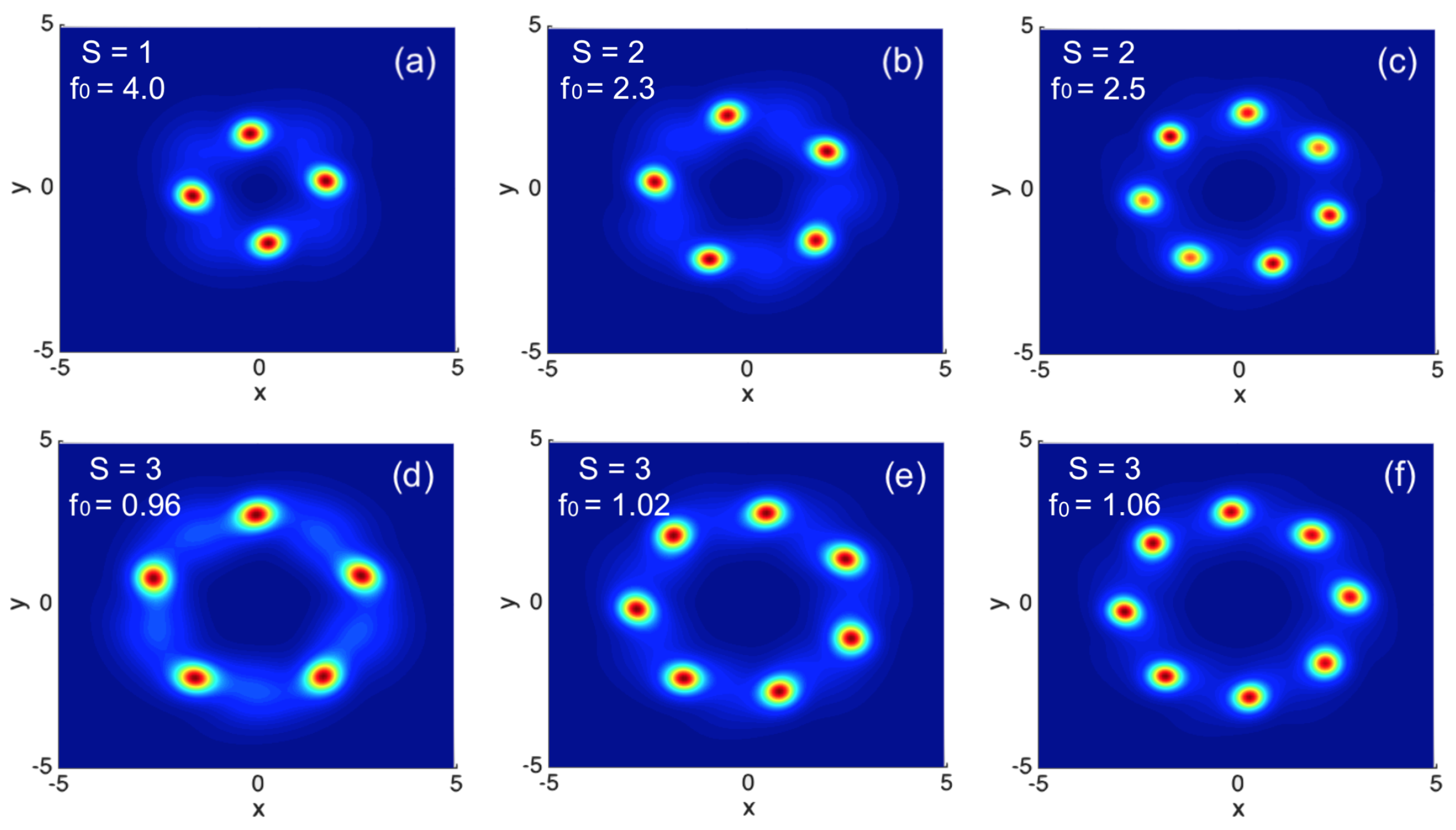
It is relevant to mention that the “traditional” azimuthal instability of vortex ring solitons with a winding number
S demonstrates the fission of the original axially symmetric shape into a set consisting of a large number
of symmetrically placed localized fragments [
2,
40], while the above examples, displayed in
Figure 3b,
Figure 5b, and
Figure 6b, demonstrate the appearance of a single bright fragment and a “garbage cloud” distributed along the original ring. At larger values of
, our simulations produced examples of the “clean” fragmentation,
viz., with
produced by the unstable vortex rings with
in
Figure 8a,
produced by
and 3 in
Figure 8b,d,
by
and 3 in
Figure 8c,e, and
by
in
Figure 8f. These outcomes of the instability development were observed at the same evolution time of
as in
Figure 3b,
Figure 5b, and
Figure 6b. The gradual increase in the number of the fragments on
S is explained by the dependence of the azimuthal index of the fastest growing eigenmode of the breaking instability on the underlying winding number
S, which is a generic property of vortex solitons [
2,
40].
Figure 8.
Examples of the fission of unstable vortex ring solitons produced by simulations of the LL Equation (
1), with
(cubic self-focusing),
(no quintic nonlinearity),
,
, and
. Each plot displays the result of the numerical simulations at time
. Values of the initial vorticity and pump’s strength are indicated in panels.
In the self-defocusing case,
, a summary of the results produced by the VA and numerical solution for the stable vortex solitons with
and 2, in the form of the dependence of their power on
, is produced in
Figure 9a (cf.
Figure 7a for
). Naturally, the VA–numerical discrepancy increases with the growth of the pump’s strength,
; see an example in
Figure 9b. Unlike the case of
, in the case of self-defocusing the vortex modes with
remained stable, at least, up to
(here, we do not consider the case of
).
Figure 9.
(a) The power versus for the vortex modes in the self-defocusing case (). The VA solutions for and 2 are shown by solid blue and dashed black lines, respectively. The corresponding numerical solutions are presented by red circles and green squares, respectively. (b) The VA-predicted and numerically obtained (the dashed red and solid blue lines, respectively) profiles of the solution with and drawn as the cross-sections through . The other parameters are , , , .
3.5. Influence of the Quintic Coefficient g
In the above analysis, the quintic term was dropped in the LL Equation (
1), thus setting
. To examine the impact of this term, we first addressed the case shown above in
Figure 3, which demonstrated that the vortex soliton with
, as a solution to Equations (
1) and (
2) with
,
and
,
, was unstable if the loss parameter fell below the critical value of
. We found that adding to Equation (
1) the quintic term with either
or
(the self-focusing or defocusing quintic nonlinearity, respectively) led to the
stabilization of the vortex mode displayed in
Figure 3, which was unstable in the absence of the quintic term. The stabilization of the soliton by quintic self-defocusing is a natural fact. More surprising is the possibility to provide the stabilization by self-focusing quintic nonlinearity because, in most cases, the inclusion of such a term gives rise to the supercritical collapse in 2D, thus making all solitons strongly unstable [
2,
40]. However, it is concluded from the stability charts displayed below in
Figure 12 that the stabilizing effect of the quintic self-focusing occurrs only at moderately small powers, for which the quintic term was not a clearly dominant one. In the general case, the soliton stability regions naturally shrunk in
Figure 12 under the action of the quintic self-focusing quintic term, with
.
In the presence of the quintic term, the comparison of the numerically found stabilized vortex soliton profiles with their VA counterparts, whose parameters were produced by a numerical solution of Equations (
18) and (
19), is presented in
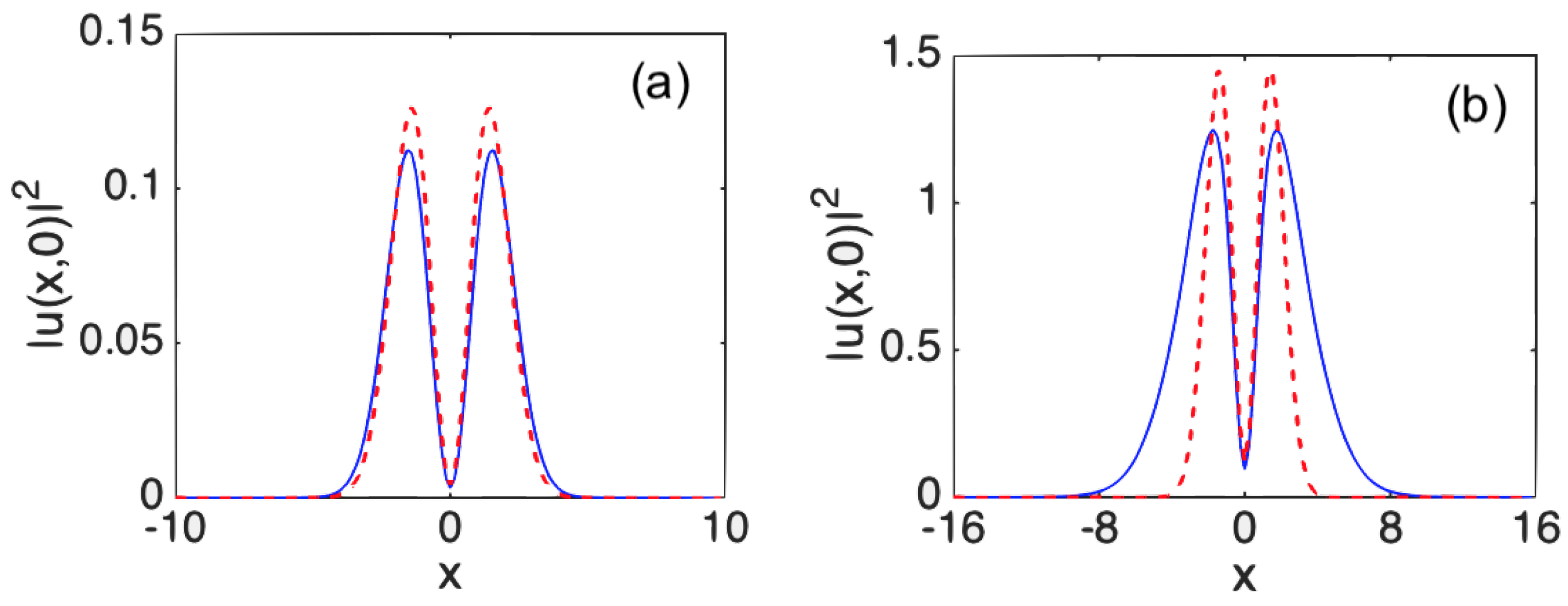
Figure 10. Similar to the results for the LL equation with the cubic-only nonlinearity, the VA is essentially more accurate in the case of the self-focusing sign of the quintic term (
) than in the opposite case, where
. In particular, in the case shown in
Figure 10, the power-measured discrepancy for
and
was, respectively,
and
. An explanation for this observation is provided by the fact that the soliton’s amplitude was much higher in the latter case.
Figure 10.
Cross-section profiles (drawn through
) for stable vortex solitns with
, produced by Equation (
1) with the quintic self-focusing
(
a) or defocusing
(
b) term. In both cases, the cubic self-focusing cubic term, with
, is present. The numerically found profiles and their VA-produced counterparts are displayed, respectively, by the solid blue and dashed lines. Other parameter are
,
, and
,
.
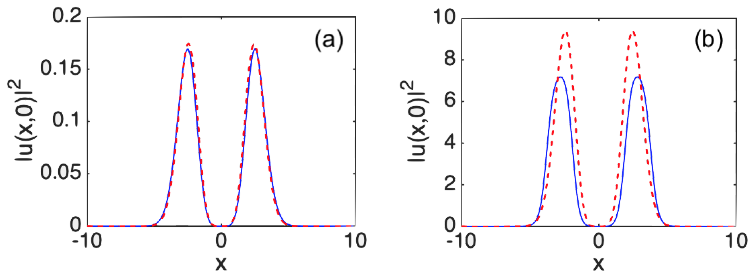
Another noteworthy finding is the stabilization of higher-vorticity solitons by the quintic term. For instance, it was shown above that, for parameters
,
,
,
,
, and
(the cubic self-focusing), all vortex solitons with
, produced by Equation (
1), were unstable. Now, we demonstrate that the soliton with
is stabilized by adding the self-defocusing quintic term with a small coefficient, just
; see
Figure 11b. As a counterintuitive effect, the stabilization of the same soliton by the self-focusing quintic term was possible too, but the necessary coefficient was large,
; see
Figure 11a (recall that
is sufficient for the stabilization of the vortex soliton with
and
in
Figure 10a). Nevertheless, similar to what has been said above, the set of
Figure 12c,f,i demonstrates the natural shrinkage of the stability area under the action of quintic self-focusing. For the stabilized vortex modes shown in
Figure 11a—in the case when both the cubic and quintic terms are self-focusing—the relative power-measured discrepancy between the numerical and VA-predicted solutions was very small,
, while in the presence of the weak quintic self-defocusing in
Figure 11b, the discrepancy was
.
Figure 11.
Cross-section profiles (drawn through
) of vortex solitons with
, stabilized by the self-focusing (
a) or defocusing (
b) quintic term in Equation (
1), with the respective coefficient
or
, with other parameters being
(cubic self-focusing),
,
, and
,
in Equation (
2). The numerically found solutions and their VA-predicted counterparts are plotted by the solid blue and dashed red lines, respectively.
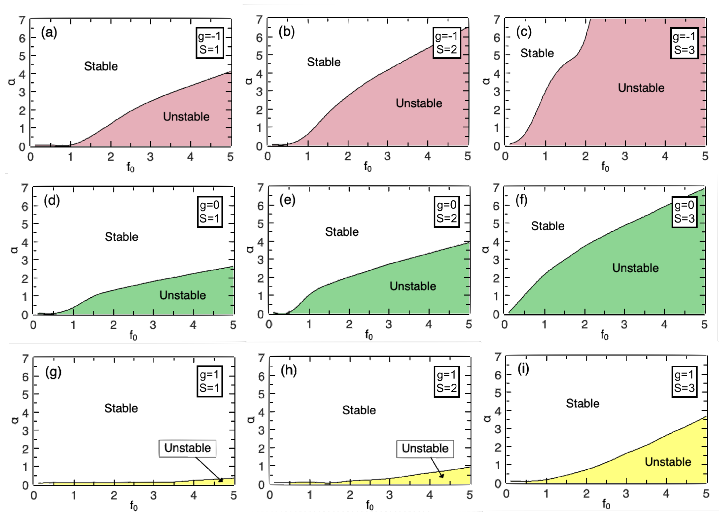
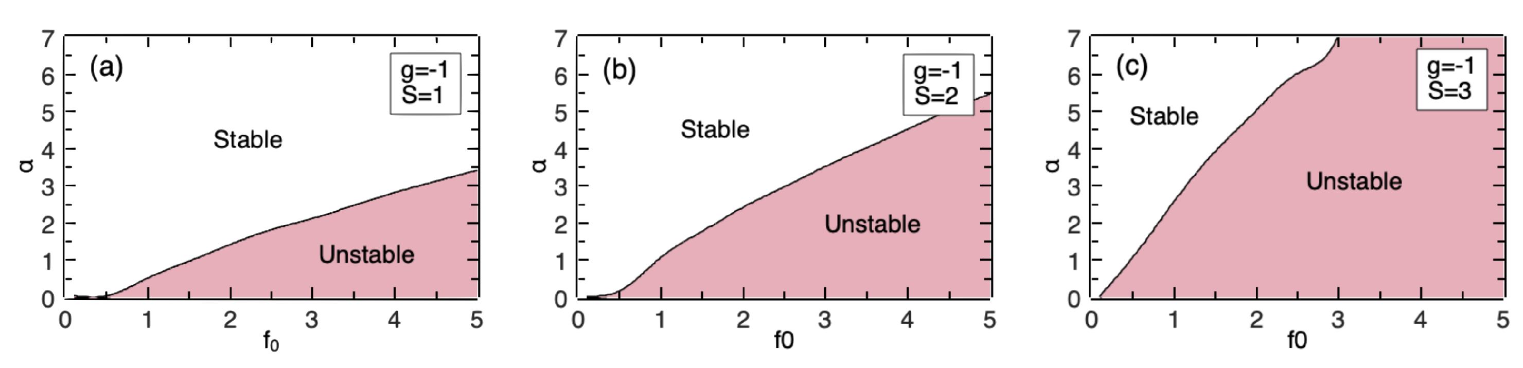
Figure 12.
Stability areas for families of the vortex solitons with winding numbers
,
and 3, in the plain of the loss coefficient (
) and amplitude of the pump beam (
), for three different values of the quintic coefficient,
(recall that
and
correspond, respectively, to the self-focusing and defocusing). Other parameters of Equations (
1) and (
2) are
(the self-focusing cubic term),
, and
.
3.6. Stability Charts in the Parameter Space
The numerical results produced in this work are summarized in the form of stability areas plotted in
Figure 12 in the parameter plane
, for the vortex soliton families with winding numbers
, 2, 3, and three values of the quintic coefficient,
, 0,
, while the cubic term is self-focusing,
, and the width of the pump beam is fixed,
. In addition to that, stability charts corresponding to the combination of the cubic self-defocusing (
) and quintic focusing (
), also for
, are plotted in
Figure 13.
Figure 13.
The same as in
Figure 12a–c but for
and
(the cubic self-defocusing and quintic focusing terms).
Figure 13.
The same as in
Figure 12a–c but for
and
(the cubic self-defocusing and quintic focusing terms).
The choice of the parameter plane
in the stability diagrams displayed in
Figure 12 is relevant, as the strength of the pump beam,
, and loss coefficient,
, are amenable to accurate adjustment in the experiment (in particular,
may be tuned by partially compensating the background loss of the optical cavity by a spatially uniform pump taken separately from the confined pump beam). As seen in all panels of
Figure 12 and
Figure 13, the increase in
naturally provides effective stabilization of the vortex modes, while none of them are stable at
, which is in agreement with the known properties of vortex soliton solutions of the 2D nonlinear Schrödinger equation with the cubic and/or cubic–quintic nonlinearity [
2,
40]. The apparent destabilization of the vortices with the increase in the pump’s amplitude
is explained by the ensuing enhancement of the destabilizing nonlinearity. Other natural features exhibited by
Figure 12 are the general stabilizing/destabilizing effect of the quintic self-defocusing/focusing (as discussed above) and expansion of the splitting instability area with the increase in
S (the latter feature is also exhibited by
Figure 13). The latter finding is natural too, as a larger
S makes the ring-shaped mode closer to the quasi-1D shape (see, in particular,
Figure 8), which facilitates the onset of the above-mentioned azimuthal MI (modulational instability).
Thus, the inference is that the instability mode, which determines the boundary of the stability areas, in
Figure 12 and
Figure 13 is the breaking of the axial symmetry of the vortex rings by azimuthal perturbations, as shown above, in particular, in
Figure 3b,
Figure 5b, and
Figure 6b. The destabilization through the spontaneous splitting of the rings into symmetric sets of fragments (see
Figure 8) occurs deeply inside the instability area, i.e., at larger values of
.
4. Conclusions
We have introduced the two-dimensional LL (Lugiato–Lefever) equation including the self-focusing or defocusing cubic or cubic–quintic nonlinearity and the confined pump with embedded vorticity (winding number), . Stable states in the form of vortex solitons (rings) for these values of S were obtained, in parallel, in the semianalytical form by means of VA (variational approximation) and numerically, by means of systematic simulations of the LL equation starting from the zero input. The VA provided much more accurate results in the case of the self-focusing nonlinearity than for the defocusing system. Stability areas of the vortex solitons with were identified in the plane of experimentally relevant parameters, viz., the pump amplitude and loss coefficient, for the self-focusing and defocusing signs of the cubic and quintic terms. Stability boundaries for the vortex rings were determined by the onset of the azimuthal instability, which broke their axial symmetry. These findings suggest new possibilities for the design of tightly confined robust optical modes, such as vortex pixels.
As an extension of this work, it may be interesting to construct solutions pinned to a symmetric pair of pump beams with or without intrinsic vorticity. In this context, it is possible to consider the beam pair with identical or opposite vorticities. In the case of the self-focusing sign of nonlinearity, one may expect an onset of spontaneous breaking of the symmetry in the dual-pump configuration. Results for this setup will be reported elsewhere.


