Enhanced Model Predictions through Principal Components and Average Least Squares-Centered Penalized Regression

Abstract

We address the estimation of regression parameters for the ill-conditioned predictive linear model in this study. Traditional least squares methods often encounter challenges in yielding reliable results when there is multicollinearity. Therefore, we employ a better shrinkage method, average least squares-centered penalized regression (ALPR), as it offers a more efficient approach for handling multicollinearity than ridge regression. Additionally, we integrate ALPR with the principal component (PC) dimension reduction method for enhanced performance. We compared the proposed PCALPR estimation technique with existing ones for ill-conditioned problems through comprehensive simulations and real-life data analyses using the mean squared error. This integration results in superior model performance compared to other methods, highlighting the potential of combining dimensionality reduction techniques with penalized regression for enhanced model predictions.

1. Introduction

Regression is a widely employed statistical methodology across various fields with different variants, including parametric, semi-, and non-parametric approaches. Linear models remain attractive due to their interpretability and the availability of tools to handle diverse data types and validate theoretical assumptions. In practice, the model predicts a response variable as a linear function of one or more predictors, for example, modelling the influence of smoking and biking habits (predictors) on the likelihood of heart disease (response). It finds application across diverse domains, including the sciences, social sciences, and the arts.

While utilizing numerous explanatory variables provides a more accurate view of the response variable, it introduces the challenge of redundant information stemming from correlations among predictors. The issue of collinearity among predictors poses a significant problem in linear regression, impacting least squares estimates, standard errors, computational accuracy, fitted values, and predictions [1,2,3,4]. Various diagnostic methods, such as the condition number, correlation analysis, eigenvalues, condition index, and the variance inflation factor, are commonly employed to identify collinearity.

Additionally, several proposed methods exist in addressing the collinearity problem, ranging from component-based methods like partial least squares regression (PLS) and principal component regression (PCR) to techniques involving penalizing solutions using the L2 norm [5,6]. The widely recognized ridge regression [7] is one such method. Different modifications to ridge regression have led to several others. These include the Liu estimator, the modified ridge-type estimator, the Kibria–Lukman estimator, the two-parameter estimator, the Stein estimator, and others [8,9,10,11,12,13]. Generally, a unanimous agreement on the optimal method is lacking, as each approach proves effective under distinct circumstances.

Recently, Wang et al. [14] developed a novel method to address multicollinearity in linear models called average least squares method (LSM)-centered penalized regression (ALPR). This method utilizes the weighted average of ordinary least squares estimators as the central point for shrinkage. Wang et al.’s [14] investigation demonstrated that ALPR outperformed ridge estimation (RE) in accuracy when the signs of the regression coefficients were consistent. Thus, ALPR is a promising method to effectively mitigate multicollinearity, especially when the signs of the regression coefficients are consistent.

Recent studies have enhanced model predictions by integrating principal components regression with some L2 norms such as ridge regression and the Stein estimator [15,16]. The PCR estimation technique stands out as a potent solution for addressing dimensionality challenges in estimation problems [17]. Known for its transparency and ease of implementation, PCR involves two pivotal steps, where the initial step applies principal component analysis (PCA) to the predictor matrix. The subsequent step entails regressing the response variable on the first principal components, which capture the most variability.

In a groundbreaking contribution, Baye and Parker [15] introduced the r-k class estimator, ingeniously combining PCR with ridge regression, resulting in a remarkable performance boost compared to using each estimator individually. This pioneering work has ignited further research, inspiring researchers to explore new avenues [18,19,20,21,22]. This paper extends the principles of PCR to the realm of average least squares method (LSM)-centered penalized regression (ALPR), giving rise to a novel method named principal component average least squares method (LSM)-centered penalized regression (PC_ALPR). The approach shares the initial step of principal component regression while diverging in the second step, where average least squares method (LSM)-centered penalized regression is used instead of the classical least squares method (LSM) to regress the response variable on the principal components.

Thus, in this study, we propose a new method to account for multicollinearity in the linear regression model by integrating principal component regression with average least squares method-centered penalized regression. This article is structured as follows: Section 2 provides a detailed review of existing methods, while Section 3 introduces a new estimator. In Section 4, we rigorously assess the new estimator’s performance through a Monte Carlo simulation study. Additionally, Section 5 showcases the practical relevance of the proposed estimator, featuring a compelling numerical example. Finally, Section 5 summarizes this research’s key findings, emphasizing the contributions of the new estimator and discussing its implications for future advancements in estimation techniques.

2. A Brief Overview of Existing Methods

Regression analysis models the connection between a response variable and one or more predictors. In this section, we will delve into the linear model, offering brief overviews of estimation methods, both with and without consideration of multicollinearity.

2.1. Least Squares Method

The linear model is a fundamental concept in statistical modelling, offering a versatile framework for understanding the relationship between a response variable and one or more predictors through a linear equation. This equation, often represented as

$$\mathrm{y}=\mathrm{X}\mathsf{\beta }+\mathsf{\epsilon },$$

(1)

captures the linear association between the response variable and predictors. In this formulation, $\mathrm{y}$ is the $\left(\mathrm{n}\times 1\right)$ vector of the response variable, $\mathrm{X}$ is the $\left(\mathrm{n}\times (\mathrm{p}+1)\right)$ matrix of predictors, and β is $\left(\mathrm{p}+1\times 1\right)$ vector of the coefficients that quantify the impact of each predictor on the response. The linear model assumes a linear and additive relationship between the predictors and the response variable. ε is an $\left(\mathrm{n}\times 1\right)$ vector of the disturbance terms, such that $\mathsf{\epsilon }~\mathrm{N}\left(0,{\mathsf{\sigma }}^2\mathrm{I}\right).$

The least squares method (LSM) stands as a cornerstone in statistical modelling, offering a powerful approach to estimating the parameters of the linear model defined in Equation (1). The primary goal of the LSM is to find the coefficients that minimize the sum of the squared differences between the observed and predicted values of the dependent variable. The vector of estimates, $\widehat{\mathsf{\beta }},$ is given by

$${\hat{\mathsf{\beta }}}_{\mathrm{L}\mathrm{S}\mathrm{M}}={\left({\mathrm{X}}^{\prime }\mathrm{X}\right)}^{-1}{\mathrm{X}}^{\prime }\mathrm{y}.$$

(2)

The variance–covariance matrix of the LSM is defined as follows:

$$\mathrm{Cov}\left(\hat{\mathsf{\beta }}\right)={\hat{\mathsf{\sigma }}}^2{\left({\mathrm{X}}^{\prime }\mathrm{X}\right)}^{-1},$$

(3)

where the mean squared error is ${\hat{\mathsf{\sigma }}}^2=\frac{{\sum }_{\mathrm{i}=1}^{\mathrm{n}}{\left({\mathrm{y}}_{\mathrm{i}}-\widehat{\mathrm{y}}\right)}^{\mathrm{e}}}{\mathrm{n}-\mathrm{r}}$. The scalar mean squared error (SMSE) of (3) is as follows:

$$\mathrm{SMSE}\left(\hat{\mathsf{\beta }}\right)={\hat{\mathsf{\sigma }}}^2{\sum }_{\mathrm{j}=1}^{\mathrm{p}}\frac{1}{{\mathrm{e}}_{\mathrm{j}}}$$

(4)

where ${\mathrm{e}}_{\mathrm{j}}$ is the eigenvalues of matrix ${\mathrm{X}}^{\prime }\mathrm{X}$.

The issue of collinearity arises when there are linear or nearly linear relationships among predictors. When exact linear relationships exist, meaning one predictor is an exact linear combination of others, the matrix ${\mathrm{X}}^{\prime }\mathrm{X}$ becomes singular, preventing a unique $\widehat{\mathsf{\beta }}$ estimate. When near-linear dependence exists among predictors, ${\mathrm{X}}^{\prime }\mathrm{X}$ is nearly singular, leading to an ill-conditioned estimation equation for regression parameters. Consequently, the parameter estimates, $\widehat{\mathsf{\beta }},$ become unstable. The variances in the regression coefficients become inflated, resulting in larger confidence intervals. In summary, the presence of collinearity, whether exact or near-linear, jeopardizes the stability of parameter estimates, leading to increased uncertainty in understanding the relationships between predictors and the response variable.

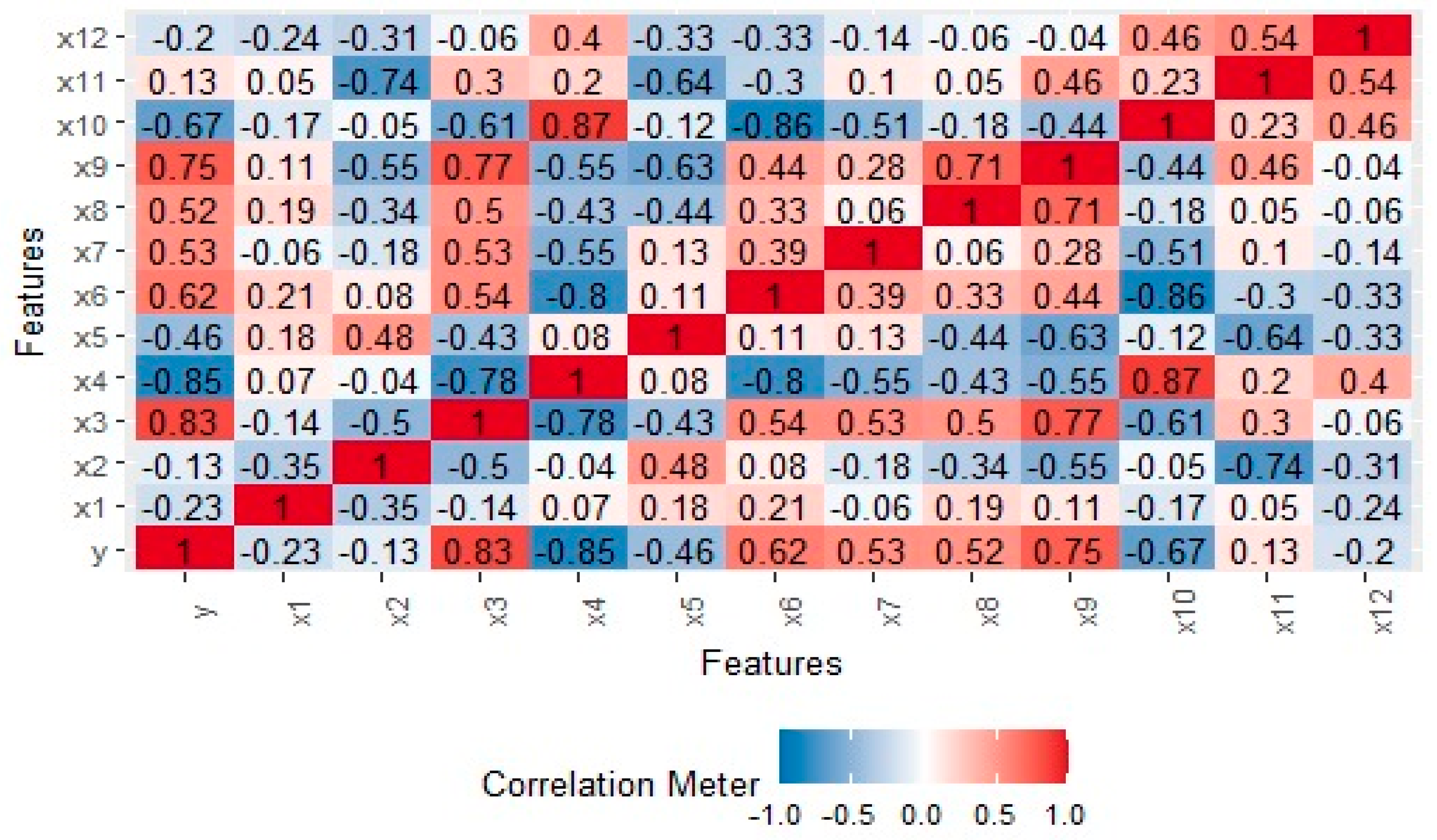
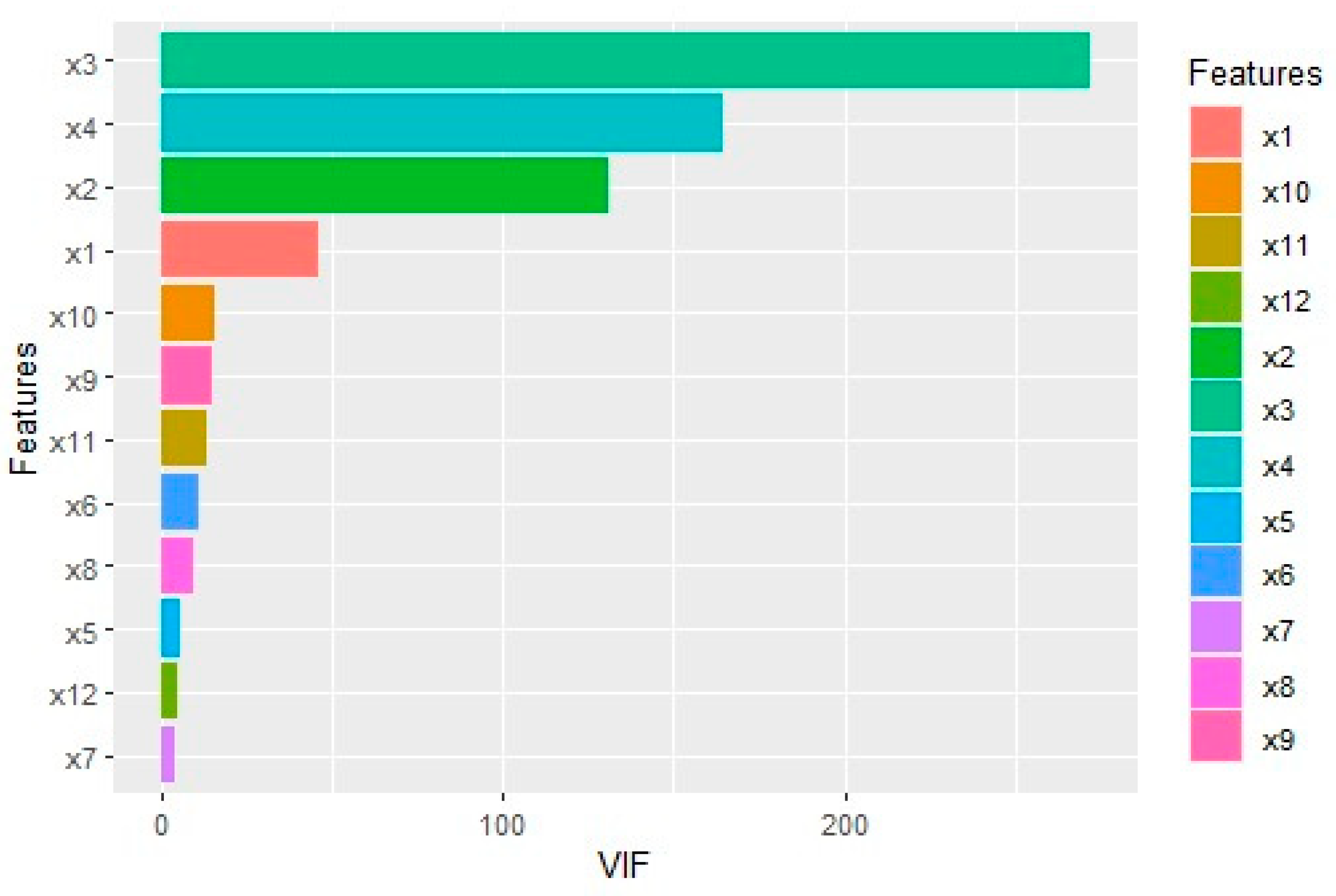
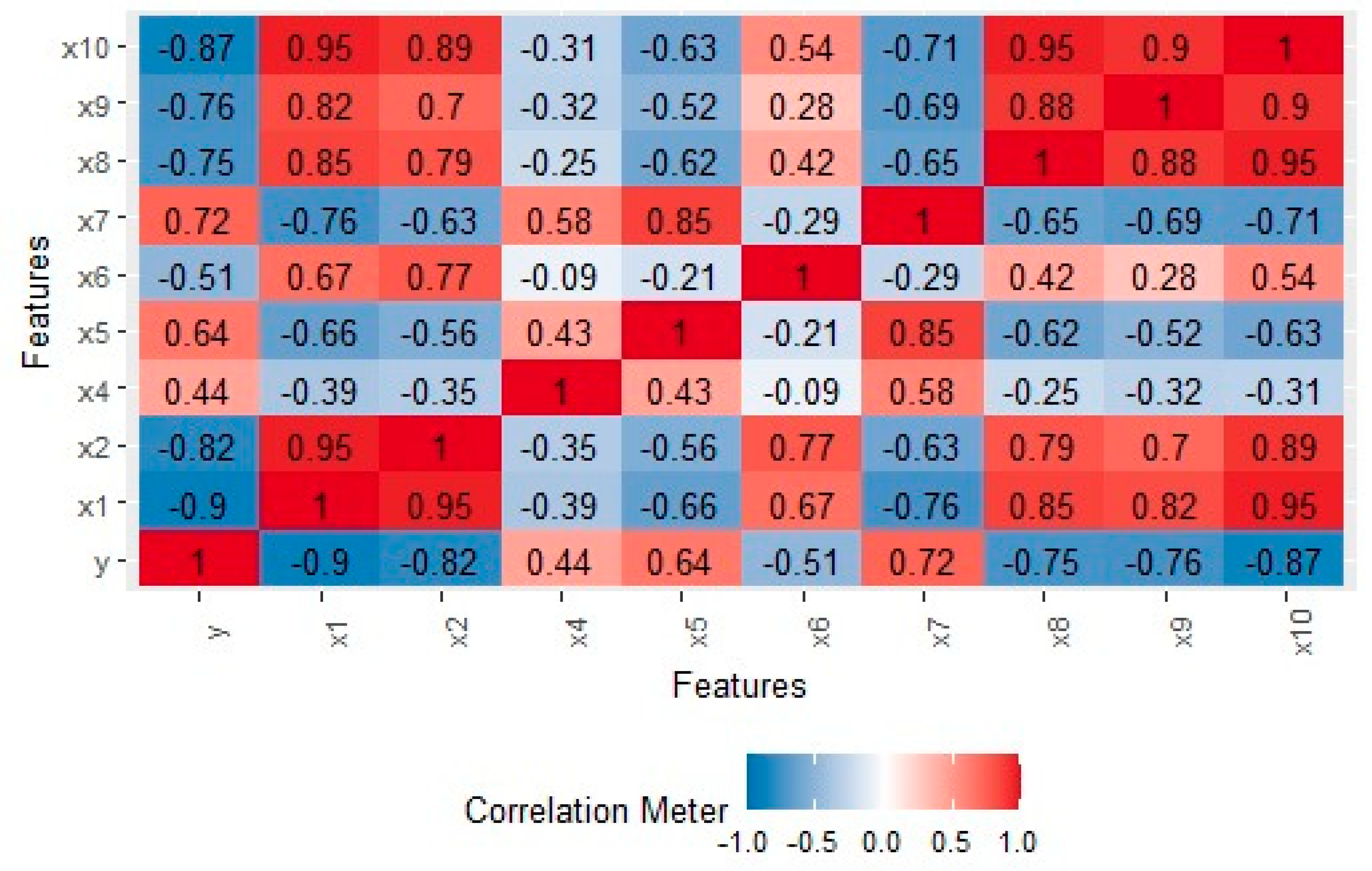
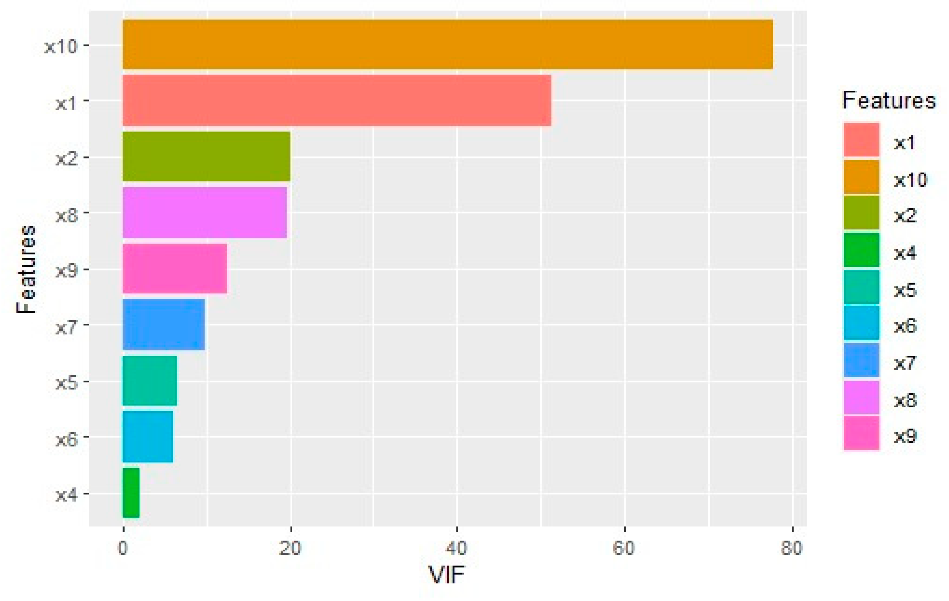
Various methods are available for detecting collinearity in linear regression models, providing insights into the interdependence among predictors. Key techniques include the following:

• Variance inflation factor (VIF): The VIF measures how much the variance of an estimated regression coefficient becomes inflated due to collinearity. A widely accepted rule of thumb suggests collinearity concerns when VIF values exceed 10.
• Condition number: The condition number assesses the sensitivity of the regression coefficients to small changes in the data. A condition number of 15 raises concerns about multicollinearity, while a number exceeding 30 indicates severe multicollinearity [3].
• Correlation matrix: Analyzing the correlation matrix of predictors helps to identify high correlations between variables. A high correlation coefficient, particularly close to 1, suggests the potential presence of collinearity.
• Eigenvalues: Investigating the eigenvalues of the predictor matrix ${\mathrm{X}}^{\prime }\mathrm{X}$ provides insights into multicollinearity. Small eigenvalues, especially near zero, indicate a higher risk of multicollinearity.

In addition to the methods for detecting collinearity in linear regression, several approaches have been proposed to address this issue effectively. These methods span a spectrum of techniques, from component-based strategies like partial least squares regression (PLS) and principal component regression (PCR) to regularization techniques involving penalizing solutions using the L2 norm. The upcoming section will offer a concise overview of a few methods developed to address collinearity. Specifically, the focus will be on techniques such as principal component regression (PCR) and the regularization methods utilizing the L2 norm.

2.2. Principal Component Regression

Principal component analysis (PCA) is a widely used dimension reduction technique to transform the original variables into a new set of uncorrelated variables, called principal components, while retaining as much of the original variability as possible [17]. The first principal component captures the maximum amount of variance in the data. Subsequent principal components capture the remaining variance while being orthogonal to each other. By retaining only the most significant principal components, PCA reduces the dimensionality of the dataset while preserving most of the original information. It is applicable in various fields, including image and signal processing, finance, and genetics. The model structure for principal component regression is obtained by transforming model (1) as follows:

$$\mathrm{y}=\mathrm{X}{\mathrm{F}}^{\prime }\mathrm{F}\mathsf{\beta }+\mathsf{\epsilon }=\mathrm{T}\mathsf{\alpha }+\mathsf{\epsilon },$$

(5)

where $\mathsf{\alpha }={\mathrm{F}}^{\prime }\mathsf{\beta },$ $\mathrm{F}=\left[{\mathrm{f}}_{\mathrm{i}},\dots ,{\mathrm{f}}_{\mathrm{p}}\right]$ is a $\mathrm{p}\times \mathrm{p}$ orthogonal matrix with ${\mathrm{F}}^{\prime }{\mathrm{X}}^{\prime }\mathrm{XF}={\mathrm{T}}^{\prime }\mathrm{T}=\mathrm{E}$ and $\mathrm{E}=\mathrm{diag}({\mathrm{e}}_{\mathrm{i}},\dots ,{\mathrm{e}}_{\mathrm{p}})$ is a $\mathrm{p}\times \mathrm{p}$ diagonal matrix of eigenvalues of ${\mathrm{X}}^{\prime }\mathrm{X}$. The score matrix T $=\mathrm{XF}=\left[{\mathrm{t}}_{\mathrm{i}},\dots ,{\mathrm{t}}_{\mathrm{p}}\right]$ has dimensions n × m, where n represents the number of observations and m represents the number of principal components. The PCR estimator of $\mathsf{\beta }$ is obtained by excluding one or more of the principal components, ${\mathrm{t}}_{\mathrm{i}}$, applying least squares method (LSM) regression to the resulting model, and then transforming the coefficients back to the original parameter space. Principal components whose eigenvalues are less than one should be excluded. These components contribute less to the overall variability of the data and can be considered less influential for prediction. However, according to Cliff [23], all components with eigenvalues greater than one should be kept for statistical inference, as they explain more variability in the data. Thus, the PCR estimator of $\mathsf{\beta }$ is defined as follows:

$${\hat{\mathsf{\beta }}}_{\mathrm{P}\mathrm{C}\mathrm{R}}={\left({\mathrm{T}}^{\prime }\mathrm{T}\right)}^{-1}{\mathrm{T}}^{\prime }\mathrm{y}.$$

(6)

2.3. Regularization Techniques

L2 norms regularization, ridge regression, is used in linear regression to address multicollinearity by penalizing the regression coefficients [7]. It involves adding a regularization term to the objective function of the least squares method (LSM). The objective function of ridge regression (RR) combines the LSM loss function with the L2 regularization term as follows:

$$\mathrm{Minimize} {‖\mathrm{y}-\mathrm{X}\mathsf{\beta }‖}_2^2+\mathrm{k}{‖\mathsf{\beta }‖}_2^2$$

(7)

where y is the vector of the response variable, X is the matrix of predictors, ${‖.‖}_2^2$ denotes the L2 norm, $\mathsf{\beta }$ is the vector of regression coefficients, and k is the regularization parameter. The regularization term penalizes regression coefficients, effectively shrinking them towards zero. Thus, there is a reduction in the variance of the parameter estimates and improved model stability, especially when there is collinearity among the predictors. The objective function in Equation (7) is expanded as follows:

$$\mathrm{Minimize} {\mathrm{y}}^{\prime }y-2{\mathsf{\beta }}^{\prime }{\mathrm{X}}^{\prime }y+{\mathsf{\beta }}^{\prime }{\mathrm{X}}^{\prime }X\mathsf{\beta }+\mathrm{k}{\mathsf{\beta }}^{\prime }\mathsf{\beta }$$

(8)

Differentiate Equation (8) with respect to $\mathsf{\beta }$ and equate to zero. Consequently,

$${\hat{\mathsf{\beta }}}_{\mathrm{R}\mathrm{R}}={\left({\mathrm{X}}^{\prime }\mathrm{X}+\mathrm{k}\mathrm{I}\right)}^{-1}{\mathrm{X}}^{\prime }\mathrm{y}.$$

(9)

According to Hoerl et al. [24], the regularization parameter, k, is defined as follows:

$$\mathrm{k}=\frac{p{\widehat{\sigma }}^2}{{\sum }_{j=1}^p{\widehat{\alpha }}_j^2}$$

(10)

The variance–covariance matrix of the ridge regression is defined as follows:

$$\mathrm{Cov}\left({\widehat{\mathsf{\beta }}}_{\mathrm{R}\mathrm{R}}\right)={\hat{\mathsf{\sigma }}}^2{\left({\mathrm{X}}^{\prime }\mathrm{X}+\mathrm{k}\mathrm{I}\right)}^{-1}{\mathrm{X}}^{\prime }\mathrm{X}{\left({\mathrm{X}}^{\prime }\mathrm{X}+\mathrm{k}\mathrm{I}\right)}^{-1}$$

(11)

The bias of the estimator is obtained as follows:

$${\mathrm{B}\mathrm{i}\mathrm{a}\mathrm{s}\left({\widehat{\mathsf{\beta }}}_{\mathrm{R}\mathrm{R}}\right)=-\mathrm{k}\left({\mathrm{X}}^{\prime }\mathrm{X}+\mathrm{k}\mathrm{I}\right)}^{-1}\mathsf{\beta }$$

(12)

Hence, the matrix mean squared error (MMSE) is given as

$$\mathrm{MMSE}\left({\widehat{\mathsf{\beta }}}_{\mathrm{R}\mathrm{R}}\right)={\hat{\mathsf{\sigma }}}^2{\left({\mathrm{X}}^{\prime }\mathrm{X}+\mathrm{k}\mathrm{I}\right)}^{-1}{\mathrm{X}}^{\prime }\mathrm{X}{\left({\mathrm{X}}^{\prime }\mathrm{X}+\mathrm{k}\mathrm{I}\right)}^{-1}+{\mathrm{k}}^2{\left({\mathrm{X}}^{\prime }\mathrm{X}+\mathrm{k}\mathrm{I}\right)}^{-1}{\mathsf{\beta }\mathsf{\beta }}^{\prime }{\left({\mathrm{X}}^{\prime }\mathrm{X}+\mathrm{k}\mathrm{I}\right)}^{-1}$$

(13)

The scalar mean squared error (SMSE) of (13) is as follows:

$$\mathrm{SMSE}\left({\widehat{\mathsf{\beta }}}_{\mathrm{R}\mathrm{R}}\right)={\hat{\mathsf{\sigma }}}^2{\sum }_{\mathrm{j}=1}^{\mathrm{p}}\frac{{\mathrm{e}}_{\mathrm{j}}}{{\left({\mathrm{e}}_{\mathrm{j}}+k\right)}^2}+{\mathrm{k}}^2{\sum }_{\mathrm{j}=1}^{\mathrm{p}}\frac{{\widehat{\alpha }}_j^2}{{\left({\mathrm{e}}_{\mathrm{j}}+k\right)}^2}$$

(14)

where $e_{\mathrm{j}}$ is the eigenvalues of matrix ${\mathrm{X}}^{\prime }\mathrm{X}$, and $\mathsf{\alpha }=\mathrm{F}\mathsf{\beta }$.

2.4. Average Least Squares Method (LSM)-Centered Penalized Regression [ALPR]

Wang et al. [14] introduced an enhanced estimator that refines the approach of ridge regression by penalizing the regression coefficients towards a predetermined constant, $\mathsf{\varsigma }$, diverging from the traditional ridge regression method that shrinks its coefficients towards zero. This modification offers a more flexible penalization framework by allowing the shrinkage target to be adjusted away from zero. The objective function of ALPR combines the LSM loss function with the L2 regularization term, which is penalized to a specific constant, $\mathsf{\varsigma }$, as follows:

$$\mathrm{Minimize} {‖\mathrm{y}-\mathrm{X}\mathsf{\beta }‖}_2^2+\mathrm{k}{‖\mathsf{\beta }-\mathsf{\varsigma }‖}_2^2$$

(15)

The objective function in Equation (15) is expanded as follows:

$$\mathrm{Minimize} {\mathrm{y}}^{\prime }y-2{\mathsf{\beta }}^{\prime }{\mathrm{X}}^{\prime }y+{\mathsf{\beta }}^{\prime }{\mathrm{X}}^{\prime }X\mathsf{\beta }+{\mathrm{k}\mathsf{\beta }}^{\prime }\mathsf{\beta }-2\mathrm{k}\mathsf{\varsigma }\mathsf{\beta }+{\mathrm{k}\mathsf{\varsigma }}^2$$

(16)

Differentiate Equation (16) with respect to $\mathsf{\beta }$ and equate to zero. Consequently,

$${\hat{\mathsf{\beta }}}_{\mathsf{\varsigma }}={\left({\mathrm{X}}^{\prime }\mathrm{X}+\mathrm{k}\mathrm{I}\right)}^{-1}\left({\mathrm{X}}^{\prime }\mathrm{y}+\mathrm{k}\mathsf{\varsigma }\right)$$

(17)

Define the distance from to $\mathsf{\beta }$ to $\mathsf{\varsigma }$ as g = $\mathsf{\beta }-\mathsf{\varsigma }$. Consequently, the objective function can be expressed as the minimization of ${‖\mathrm{y}-\mathrm{X}\mathsf{\beta }‖}_2^2+\mathrm{k}{‖\mathrm{g}‖}_2^2$, akin to the formulation of ridge regression. Let $\mathsf{\alpha }=\mathrm{Fg}$. Thus, the scalar mean squared error (SMSE) is as follows:

$$\mathrm{SMSE}\left({\widehat{\mathsf{\beta }}}_{\mathsf{\varsigma }}\right)={\hat{\mathsf{\sigma }}}^2{\sum }_{\mathrm{j}=1}^{\mathrm{p}}\frac{{\mathrm{e}}_{\mathrm{j}}}{{\left({\mathrm{e}}_{\mathrm{j}}+k\right)}^2}+{\mathrm{k}}^2{\sum }_{\mathrm{j}=1}^{\mathrm{p}}\frac{{\widehat{\alpha }}_j^2}{{\left({\mathrm{e}}_{\mathrm{j}}+k\right)}^2}$$

(18)

Consequently, as ${\hat{\alpha }}_j^2$ increases, the $\mathrm{SMSE}\left({\widehat{\mathsf{\beta }}}_{\mathsf{\varsigma }}\right)$ also increases. Equation (18), being independent of F, roughly indicates that a smaller g, i.e., the closer $\mathsf{\beta }$ is to c, resulting in a smaller $\mathrm{SMSE}\left({\widehat{\mathsf{\beta }}}_{\mathsf{\varsigma }}\right)$, implying better estimation. While least squares method (LSM) estimators may suffer from instability when there is significant multicollinearity among explanatory variables, their average values demonstrate reduced susceptibility to multicollinearity effects. As an alternative to the conventional shrinkage center of zero used in ridge regression (RR), employing the average value of ${\hat{\mathsf{\beta }}}_{\mathrm{g}}$ as a shrinkage center offers a more appropriate solution. This innovative approach, termed Average OLS Penalized Regression (AOPR), relies on a p-dimensional vector, d, where all elements are set to 1, to define ${\mathsf{\varsigma }}_M$ as the average of the ${\hat{\mathsf{\beta }}}_{\mathrm{g}}$. Consequently, the shrinkage center for ALPR, ${\mathsf{\varsigma }}_M$, is established as ${\mathsf{\varsigma }}_M={\mathsf{\varsigma }}_{M}d$. To ensure a stable estimation of ${\mathsf{\varsigma }}_M$ that maximizes explanatory power for the observed, ${\mathsf{\varsigma }}_M$ can be estimated through a specific procedure designed to enhance its stability and explanatory capacity. This meticulous procedure ensures that AOPR provides robust and effective regression results, particularly in scenarios with high multicollinearity among predictor variables. Thus, ${\mathsf{\varsigma }}_M$ is estimated by minimizing ${‖\mathrm{y}-\mathrm{X}{\mathsf{\varsigma }}_{\mathrm{M}}‖}_2^2.\mathrm{Hence},{\mathsf{\varsigma }}_{\mathrm{M}}=\mathrm{d}{\left({\mathrm{d}}^{\prime }{\mathrm{X}}^{\prime }\mathrm{X}\mathrm{d}\right)}^{-1}{\mathrm{d}}^{\prime }{\mathrm{X}}^{\prime }\mathrm{X}{\hat{\mathsf{\beta }}}_{\mathrm{L}\mathrm{S}\mathrm{M}}.$ Let ${{\mathsf{\varsigma }}^{^}}_{\mathrm{M}}$ replace the constant $\mathsf{\varsigma }$ in Equation (17); then, we have

$${\hat{\mathsf{\beta }}}_{\mathrm{A}\mathrm{L}\mathrm{P}\mathrm{R}}={\left({\mathrm{X}}^{\prime }\mathrm{X}+\mathrm{k}\mathrm{I}\right)}^{-1}\left({\mathrm{X}}^{\prime }\mathrm{y}+\mathrm{k}\mathrm{d}{\left({\mathrm{d}}^{\prime }{\mathrm{X}}^{\prime }\mathrm{X}\mathrm{d}\right)}^{-1}{\mathrm{d}}^{\prime }{\mathrm{X}}^{\prime }\mathrm{X}{\widehat{\mathsf{\beta }}}_{\mathrm{L}\mathrm{S}\mathrm{M}}\right)$$

$${=\left({\mathrm{X}}^{\prime }\mathrm{X}+\mathrm{k}\mathrm{I}\right)}^{-1}\left({\mathrm{X}}^{\prime }\mathrm{X}+\mathrm{k}\mathrm{d}{\left({\mathrm{d}}^{\prime }{\mathrm{X}}^{\prime }\mathrm{X}\mathrm{d}\right)}^{-1}{\mathrm{d}}^{\prime }{\mathrm{X}}^{\prime }\mathrm{X}\right){\hat{\mathsf{\beta }}}_{\mathrm{L}\mathrm{S}\mathrm{M}}$$

(19)

$$=\mathrm{Q}{\hat{\mathsf{\beta }}}_{\mathrm{L}\mathrm{S}\mathrm{M}}\mathrm{where}{\left({\mathrm{X}}^{\prime }\mathrm{X}+\mathrm{k}\mathrm{I}\right)}^{-1}\left({\mathrm{X}}^{\prime }\mathrm{X}+\mathrm{k}\mathrm{d}{\left({\mathrm{d}}^{\prime }{\mathrm{X}}^{\prime }\mathrm{X}\mathrm{d}\right)}^{-1}{\mathrm{d}}^{\prime }{\mathrm{X}}^{\prime }\mathrm{X}\right)$$

The covariance matrix of ${\hat{\mathsf{\beta }}}_{\mathrm{A}\mathrm{L}\mathrm{P}\mathrm{R}}$ is as follows:

$$\mathrm{Cov}\left({\widehat{\mathsf{\beta }}}_{\mathrm{A}\mathrm{L}\mathrm{P}\mathrm{R}}\right)={\hat{\mathsf{\sigma }}}^2\mathrm{Q}{\left({\mathrm{X}}^{\prime }\mathrm{X}\right)}^{-1}{\mathrm{Q}}^{\prime }$$

(20)

Following Wang et al. [14], let $\mathrm{h}=\mathrm{Fd}{\left({\mathrm{d}}^{\prime }{\mathrm{X}}^{\prime }\mathrm{X}\mathrm{d}\right)}^{-1}{\mathrm{d}}^{\prime }{\mathrm{X}}^{\prime }\mathrm{X}{\mathrm{F}}^{\prime }$ and $t_j=b_j^2+{\sum }_{j=1}^p\left(h_{ij}^2\frac{{\sigma }^2}{e_j}+h_{ij}^2{b}_j^2\right)-2b_j{h}_j^{\prime }b$, where $h_i$ is the ith row vector of h. Consequently, the SMSE of ${\hat{\mathsf{\beta }}}_{\mathrm{A}\mathrm{L}\mathrm{P}\mathrm{R}}$ is as follows:

$$\mathrm{SMSE}\left({\widehat{\mathsf{\beta }}}_{\mathrm{A}\mathrm{L}\mathrm{P}\mathrm{R}}\right)={\hat{\mathsf{\sigma }}}^2{\sum }_{\mathrm{j}=1}^{\mathrm{p}}\frac{{\mathrm{e}}_{\mathrm{j}}+2k{h}_{jj}}{{\left({\mathrm{e}}_{\mathrm{j}}+k\right)}^2}+{\mathrm{k}}^2{\sum }_{\mathrm{j}=1}^{\mathrm{p}}\frac{t_j}{{\left({\mathrm{e}}_{\mathrm{j}}+k\right)}^2}$$

(21)

where $\left\{\begin{array}{c}k\le \frac{{\mathrm{e}}_{\mathrm{j}}{\widehat{\mathsf{\sigma }}}^2-{\widehat{\mathsf{\sigma }}}^2{{\mathrm{e}}_{\mathrm{j}}h}_{jj}}{{\mathrm{e}}_{\mathrm{j}}{t}_j-{\widehat{\mathsf{\sigma }}}^2{h}_{jj}},{\mathrm{e}}_{\mathrm{j}}{t}_j-{\widehat{\mathsf{\sigma }}}^2{h}_{jj}>0\\ k\ge \frac{{\mathrm{e}}_{\mathrm{j}}{\widehat{\mathsf{\sigma }}}^2-{\widehat{\mathsf{\sigma }}}^2{{\mathrm{e}}_{\mathrm{j}}h}_{jj}}{{\mathrm{e}}_{\mathrm{j}}{t}_j-{\widehat{\mathsf{\sigma }}}^2{h}_{jj}},{\mathrm{e}}_{\mathrm{j}}{t}_j-{\widehat{\mathsf{\sigma }}}^2{h}_{jj}<0\end{array}\right.$

Set ${\mathrm{l}}_{\mathrm{j}}=\left\{\begin{array}{c}0,{\mathrm{e}}_{\mathrm{j}}{t}_j-{\widehat{\mathsf{\sigma }}}^2{h}_{jj}\le 0\mathrm{and}{h}_{jj}>1\\ max\left[0,\frac{{\mathrm{e}}_{\mathrm{j}}{\widehat{\mathsf{\sigma }}}^2-{\widehat{\mathsf{\sigma }}}^2{{\mathrm{e}}_{\mathrm{j}}h}_{jj}}{{\mathrm{e}}_{\mathrm{j}}{t}_j-{\widehat{\mathsf{\sigma }}}^2{h}_{jj}}\right],{\mathrm{e}}_{\mathrm{j}}{t}_j-{\widehat{\mathsf{\sigma }}}^2{h}_{jj}<0\end{array}\right.$

Wang et al. [14] proposed that setting k = ${\mathrm{l}}_{\mathrm{m}\mathrm{i}\mathrm{n}}$ serves as the optimal choice for the shrinkage parameter in ALPR. For further insights, we advise consulting the works of Wang et al. [14,25]. These references provide an in-depth exploration and analysis of the optimal shrinkage parameter selection in ALPR.

2.5. Principal Component Average LSM-Centered Penalized Regression

In this section, we introduce a novel hybrid estimation approach that integrates principal component regression (PCR) with average LSM-centered penalized regression (ALPR) to create the principal component average LSM-centered penalized regression method. We aim to capitalize on the strengths of PCR and ALPR to enhance the modelling process and boost predictive accuracy by combining these two techniques. The methodology comprises the following steps:

• Standardization of predictor variables to ensure comparability, with a mean of zero and unit variance.
• Perform principal component analysis (PCA) on the predictor variables.
• Selection of principal components corresponding to eigenvalues exceeding 1, as they explain more variance than an individual predictor variable [23,26].
• Regression of the response variable on the chosen principal components to derive fitted values.
• Replace the original response variable with the fitted values obtained from the PCR model.
• Utilization of average LSM-centered penalized regression to regress the transformed response variable (fitted values from step iv) along with the original predictor variables.
• Evaluation of the combined approach’s performance using appropriate metrics such as the scalar mean squared error (SMSE) and predicted mean squared error.

Mathematically, Baye and Parker [15] integrated the principal component with the ridge estimator to form principal component ridge regression (PCRR). PCRR according to Chang and Yang [19] is defined as follows:

$${\hat{\mathsf{\beta }}}_{\mathrm{P}\mathrm{C}\mathrm{R}\mathrm{R}}={\left({\mathrm{T}}^{\prime }\mathrm{T}+\mathrm{k}\mathrm{I}\right)}^{-1}{\mathrm{T}}^{\prime }\mathrm{y}.$$

(22)

The scalar mean squared error (SMSE) is as follows:

$$\mathrm{SMSE}\left({\widehat{\mathsf{\beta }}}_{\mathrm{P}\mathrm{C}\mathrm{R}\mathrm{R}}\right)={\hat{\mathsf{\sigma }}}^2{\sum }_{\mathrm{j}=1}^{\mathrm{r}}\frac{{\mathrm{e}}_{\mathrm{j}}}{{\left({\mathrm{e}}_{\mathrm{j}}+k\right)}^2}+{\mathrm{k}}^2{\sum }_{\mathrm{j}=1}^r\frac{{\widehat{\alpha }}_j^2}{{\left({\mathrm{e}}_{\mathrm{j}}+k\right)}^2}$$

(23)

where r $\le p.$ Thus, the proposed estimator is defined as follows:

$${\hat{\mathsf{\beta }}}_{\mathrm{P}\mathrm{C}\mathrm{A}\mathrm{L}\mathrm{P}\mathrm{R}}={\left(\mathrm{T}+\mathrm{k}\mathrm{I}\right)}^{-1}\left({\mathrm{T}}^{\prime }\mathrm{y}+\mathrm{k}\mathrm{d}{\left({\mathrm{d}}^{\prime }\mathrm{T}\mathrm{d}\right)}^{-1}{\mathrm{d}}^{\prime }\mathrm{T}{\widehat{\mathsf{\beta }}}_{\mathrm{P}\mathrm{C}\mathrm{R}}\right).$$

(24)

The scalar mean squared error (SMSE) is as follows:

$$\mathrm{SMSE}\left({\widehat{\mathsf{\beta }}}_{\mathrm{P}\mathrm{C}\mathrm{A}\mathrm{L}\mathrm{P}\mathrm{R}}\right)={\hat{\mathsf{\sigma }}}^2{\sum }_{\mathrm{j}=1}^{\mathrm{r}}\frac{{\mathrm{e}}_{\mathrm{j}}+2k{h}_{jj}}{{\left({\mathrm{e}}_{\mathrm{j}}+k\right)}^2}+{\mathrm{k}}^2{\sum }_{\mathrm{j}=1}^{\mathrm{r}}\frac{t_j}{{\left({\mathrm{e}}_{\mathrm{j}}+k\right)}^2}$$

(25)

3. Simulation

This section will examine a simulation study that evaluates the performance of the proposed estimator in comparison to existing estimators, across various levels of multicollinearity. The simulation study is conducted using RStudio, a popular integrated development environment for R programming. We follow a specific data generation mechanism to account for the number of correlated variables. We generate the number of $\mathrm{n}\in \left\{30,50,100,200\right\}$ observations with $\mathrm{p}\in \left\{3,7\right\}$ explanatory variables using the following scheme:

$${\mathrm{x}}_{\mathrm{i}\mathrm{j}}=\left\{\begin{array}{cc}{\left(1-{\mathsf{\gamma }}^2\right)}^{\frac{1}{2}}{\mathrm{w}}_{\mathrm{i}\mathrm{j}}+\mathsf{\gamma }{\mathrm{w}}_{\mathrm{i}\left(\mathrm{p}+1\right)},& \mathrm{i}=\mathrm{1,2},\dots ,\mathrm{n},\mathrm{j}=\mathrm{1,2},\dots ,\mathrm{m}\end{array}\right.$$

(26)

where ${\mathrm{w}}_{\mathrm{i}\mathrm{j}}$ represents independent standard normal pseudo-random numbers; $\mathrm{m}\in \left\{\mathrm{2,3},\dots ,\mathrm{p}\right\}$ is the number of correlated variables. The variables are standardized, and thus, $\mathrm{X}\mathrm{\text{'}}\mathrm{y}$ shows the correlation. Furthermore, we consider moderate and strong collinearity levels using ${\mathsf{\gamma }}^2\in \left\{0.8, 0.9, 0.99, \mathrm{and} 0.999\right\}$. We generate the model observations following Equation (1) with $\mathsf{\epsilon }\sim \mathrm{N}\left(0,{\mathsf{\sigma }}^2\mathrm{I}\right)$, ${\mathsf{\sigma }}^2\in \left\{25,100\right]$. The response variable is a linear function of the predictors generated in (26) with coefficients ${\mathsf{\beta }}_1,{\mathsf{\beta }}_2,\dots ,{\mathsf{\beta }}_{\mathrm{p}},\mathrm{r}\mathrm{e}\mathrm{s}\mathrm{p}\mathrm{e}\mathrm{c}\mathrm{t}\mathrm{i}\mathrm{v}\mathrm{e}\mathrm{l}\mathrm{y}.$ The model assumes a zero intercept, and the values of $\mathsf{\beta }$ are chosen such that ${\sum }_{j=1}^p{\beta }_j^2=1$. We repeat the whole data generation process 1000 times and evaluate the estimator’s performance using the mean squared error (MSE) and prediction mean squared error (PMSE), respectively, given by

$$\begin{array}{c}\mathrm{M}\mathrm{S}\mathrm{E}=\frac{1}{1000}{\sum }_{\mathrm{i}=1}^{1000}{\left({\widehat{\mathsf{\beta }}}_{\mathrm{*}}^{\left(\mathrm{i}\right)}-\mathsf{\beta }\right)}^{\prime }\left({\widehat{\mathsf{\beta }}}_{\mathrm{*}}^{\left(\mathrm{i}\right)}-\mathsf{\beta }\right)\\ \mathrm{P}\mathrm{M}\mathrm{S}\mathrm{E}=\frac{1}{1000}{\sum }_{\mathrm{j}=1}^{1000}{\left({\widehat{\mathrm{y}}}_{\mathrm{*}}^{\left(\mathrm{j}\right)}-{\mathrm{y}}_{\mathrm{*}}\right)}^{\prime }\left({\widehat{\mathrm{y}}}_{\mathrm{*}}^{\left(\mathrm{j}\right)}-{\mathrm{y}}_{\mathrm{*}}\right)\end{array}$$

(27)

where ${\widehat{\mathsf{\beta }}}_{\mathrm{*}}^{\left(\mathrm{i}\right)}$ is any of the existing estimators or the proposed estimator. Further, ${\widehat{\mathrm{y}}}_{\mathrm{*}}=\mathrm{X}{\widehat{\mathsf{\beta }}}_{\mathrm{*}}$.

The simulation results are available in

Table 1. Estimated MSE values for p = 3 with $\mathsf{\sigma }$ = 5.

Estimators	Sample Size (n)
	40		50		100		200
	MSE	PMSE	MSE	PMSE	MSE	PMSE	MSE	PMSE
$\mathit{\rho }\mathbf{=}\mathbf{0.8}$
${\widehat{\mathit{\alpha }}}_{\mathit{L}\mathit{S}\mathit{M}}$	4.5703	1.8058	3.7860	1.5066	1.4439	0.7212	0.7814	0.3768
${\widehat{\mathit{\alpha }}}_{\mathit{R}\mathit{R}}$	0.7274	1.3422	0.6345	1.5999	0.5705	1.5833	0.5235	1.1366
${\widehat{\mathit{\alpha }}}_{\mathit{P}\mathit{C}\mathit{R}\mathit{R}}$	0.6994	1.3336	0.6102	1.5923	0.5629	1.5807	0.5176	1.1345
${\widehat{\mathit{\alpha }}}_{\mathit{A}\mathit{L}\mathit{P}\mathit{R}}$	0.3408	0.6067	0.2077	0.4857	0.0990	0.2578	0.0612	0.1213
${\widehat{\mathit{\alpha }}}_{\mathit{P}\mathit{C}\mathit{A}\mathit{L}\mathit{P}\mathit{R}}$	0.3091	0.5961	0.1835	0.4785	0.0913	0.2550	0.0548	0.1190
$\mathit{\rho }\mathbf{=}\mathbf{0.9}$
${\widehat{\mathit{\alpha }}}_{\mathit{L}\mathit{S}\mathit{M}}$	8.2602	1.8084	6.9663	1.5057	2.6458	0.7200	1.4272	0.3756
${\widehat{\mathit{\alpha }}}_{\mathit{R}\mathit{R}}$	0.6386	1.3292	0.5172	1.5299	0.4680	1.4253	0.4303	1.0351
${\widehat{\mathit{\alpha }}}_{\mathit{P}\mathit{C}\mathit{R}\mathit{R}}$	0.5867	1.3208	0.4749	1.5230	0.4565	1.4232	0.4218	1.0335
${\widehat{\mathit{\alpha }}}_{\mathit{A}\mathit{L}\mathit{P}\mathit{R}}$	0.3194	0.6107	0.1921	0.4846	0.0935	0.2558	0.0572	0.1191
${\widehat{\mathit{\alpha }}}_{\mathit{P}\mathit{C}\mathit{A}\mathit{L}\mathit{P}\mathit{R}}$	0.2661	0.6019	0.1501	0.4779	0.0820	0.2537	0.0486	0.1175
$\mathit{\rho }\mathbf{=}\mathbf{0.99}$
${\widehat{\mathit{\alpha }}}_{\mathit{L}\mathit{S}\mathit{M}}$	75.5686	1.8135	65.0997	1.5068	24.5618	0.7180	13.2297	0.3742
${\widehat{\mathit{\alpha }}}_{\mathit{R}\mathit{R}}$	0.7584	0.7546	0.5639	0.7169	0.2559	0.5629	0.2045	0.3998
${\widehat{\mathit{\alpha }}}_{\mathit{P}\mathit{C}\mathit{R}\mathit{R}}$	0.2983	0.7466	0.1953	0.7106	0.1708	0.5613	0.1492	0.3987
${\widehat{\mathit{\alpha }}}_{\mathit{A}\mathit{L}\mathit{P}\mathit{R}}$	0.7064	0.6182	0.5047	0.4852	0.1625	0.2534	0.0993	0.1169
${\widehat{\mathit{\alpha }}}_{\mathit{P}\mathit{C}\mathit{A}\mathit{L}\mathit{P}\mathit{R}}$	0.2460	0.6103	0.1365	0.4789	0.0774	0.2518	0.0440	0.1158
$\mathit{\rho }\mathbf{=}\mathbf{0.999}$
${\widehat{\mathit{\alpha }}}_{\mathit{L}\mathit{S}\mathit{M}}$	747.4641	1.8152	646.6567	1.5075	243.8220	0.7174	131.3629	0.3739
${\widehat{\mathit{\alpha }}}_{\mathit{R}\mathit{R}}$	4.8993	0.6013	3.8973	0.4959	0.9154	0.2828	0.5841	0.1504
${\widehat{\mathit{\alpha }}}_{\mathit{P}\mathit{C}\mathit{R}\mathit{R}}$	0.3800	0.5934	0.2714	0.4897	0.0951	0.2812	0.0574	0.1493
${\widehat{\mathit{\alpha }}}_{\mathit{A}\mathit{L}\mathit{P}\mathit{R}}$	4.9065	0.6208	3.8943	0.4858	0.9060	0.2528	0.5716	0.1165
${\widehat{\mathit{\alpha }}}_{\mathit{P}\mathit{C}\mathit{A}\mathit{L}\mathit{P}\mathit{R}}$	0.3869	0.6129	0.2688	0.4796	0.0859	0.2512	0.0448	0.1154

Least squares method (LSM), ridge regression (RR), principal components ridge regression (PCRR), average least squares method-centered penalized regression (ALPR), and principal component average least squares method-centered penalized regression (PCALPR).

,

Table 2. Estimated MSE values for p = 3 with $\mathsf{\sigma }$ = 10.

Estimators	Sample Size (n)
	40		50		100		200
	MSE	PMSE	MSE	PMSE	MSE	PMSE	MSE	PMSE
$\mathit{\rho }\mathbf{=}\mathbf{0.8}$
${\widehat{\mathit{\alpha }}}_{\mathit{L}\mathit{S}\mathit{M}}$	18.2811	7.2231	15.1442	6.0263	5.7757	2.8849	3.1255	1.5073
${\widehat{\mathit{\alpha }}}_{\mathit{R}\mathit{R}}$	0.9168	1.7485	0.8824	2.2964	0.8793	2.4704	0.8848	1.9435
${\widehat{\mathit{\alpha }}}_{\mathit{P}\mathit{C}\mathit{R}\mathit{R}}$	0.9085	1.7460	0.8752	2.2942	0.8776	2.4698	0.8838	1.9431
${\widehat{\mathit{\alpha }}}_{\mathit{A}\mathit{L}\mathit{P}\mathit{R}}$	1.2426	2.3914	0.7333	1.9121	0.3638	1.0202	0.2172	0.4750
${\widehat{\mathit{\alpha }}}_{\mathit{P}\mathit{C}\mathit{A}\mathit{L}\mathit{P}\mathit{R}}$	1.2280	2.3798	0.7269	1.9115	0.3619	1.0188	0.2160	0.4744
$\mathit{\rho }\mathbf{=}\mathbf{0.9}$
${\widehat{\mathit{\alpha }}}_{\mathit{L}\mathit{S}\mathit{M}}$	33.0407	7.2338	27.8653	6.0229	10.5832	2.8800	5.7089	1.5024
${\widehat{\mathit{\alpha }}}_{\mathit{R}\mathit{R}}$	0.8673	1.9343	0.8025	2.5496	0.8090	2.5199	0.8207	2.0128
${\widehat{\mathit{\alpha }}}_{\mathit{P}\mathit{C}\mathit{R}\mathit{R}}$	0.8513	1.9317	0.7895	2.5475	0.8061	2.5194	0.8189	2.0124
${\widehat{\mathit{\alpha }}}_{\mathit{A}\mathit{L}\mathit{P}\mathit{R}}$	1.0717	2.4100	0.6032	1.9110	0.3275	1.0150	0.1932	0.4697
${\widehat{\mathit{\alpha }}}_{\mathit{P}\mathit{C}\mathit{A}\mathit{L}\mathit{P}\mathit{R}}$	1.0541	2.4058	0.5907	1.9096	0.3245	1.0142	0.1914	0.4692
$\mathit{\rho }\mathbf{=}\mathbf{0.99}$
${\widehat{\mathit{\alpha }}}_{\mathit{L}\mathit{S}\mathit{M}}$	302.2745	7.2540	260.3987	6.0271	98.2470	2.8721	52.9188	1.4969
${\widehat{\mathit{\alpha }}}_{\mathit{R}\mathit{R}}$	0.7899	1.6973	0.5868	1.8439	0.4718	1.4856	0.4570	1.1875
${\widehat{\mathit{\alpha }}}_{\mathit{P}\mathit{C}\mathit{R}\mathit{R}}$	0.6424	1.6947	0.4689	1.8418	0.4475	1.4852	0.4415	1.1872
${\widehat{\mathit{\alpha }}}_{\mathit{A}\mathit{L}\mathit{P}\mathit{R}}$	1.0686	2.4428	0.6042	1.9164	0.3278	1.0074	0.1882	0.4634
${\widehat{\mathit{\alpha }}}_{\mathit{P}\mathit{C}\mathit{A}\mathit{L}\mathit{P}\mathit{R}}$	0.9207	2.4403	0.4866	1.9144	0.3035	1.0069	0.1727	0.4631
$\mathit{\rho }\mathbf{=}\mathbf{0.999}$
${\widehat{\mathit{\alpha }}}_{\mathit{L}\mathit{S}\mathit{M}}$	2989.8565	7.2607	2586.6267	6.0300	975.2882	2.8697	525.4517	1.4957
${\widehat{\mathit{\alpha }}}_{\mathit{R}\mathit{R}}$	2.2111	1.9215	1.6236	1.7000	0.5257	0.9417	0.3502	0.5326
${\widehat{\mathit{\alpha }}}_{\mathit{P}\mathit{C}\mathit{R}\mathit{R}}$	0.7559	1.9189	0.4611	1.6980	0.2885	0.9412	0.1977	0.5322
${\widehat{\mathit{\alpha }}}_{\mathit{A}\mathit{L}\mathit{P}\mathit{R}}$	2.4064	2.4533	1.6764	1.9192	0.5447	1.0052	0.3241	0.4620
${\widehat{\mathit{\alpha }}}_{\mathit{P}\mathit{C}\mathit{A}\mathit{L}\mathit{P}\mathit{R}}$	0.9509	2.4507	0.5142	1.9172	0.3076	1.0047	0.1716	0.4617

Least squares method (LSM), ridge regression (RR), principal components ridge regression (PCRR), average least squares method-centered penalized regression (ALPR), and principal component average least squares method-centered penalized regression (PCALPR).

,

Table 3. Estimated MSE values for p = 7 with $\mathsf{\sigma }$ = 5.

Estimators	Sample Size (n)
	40		50		100		200
	MSE	PMSE	MSE	PMSE	MSE	PMSE	MSE	PMSE
$\mathit{\rho }\mathbf{=}\mathbf{0.8}$
${\widehat{\mathit{\alpha }}}_{\mathit{L}\mathit{S}\mathit{M}}$	12.6808	4.3744	10.7662	3.5549	4.4001	1.7374	2.2289	0.8519
${\widehat{\mathit{\alpha }}}_{\mathit{R}\mathit{R}}$	0.6043	1.8219	0.4060	2.2655	0.4646	1.9878	0.4255	1.6291
${\widehat{\mathit{\alpha }}}_{\mathit{P}\mathit{C}\mathit{R}\mathit{R}}$	0.5461	1.7997	0.3676	2.2523	0.4552	1.9848	0.4251	1.6289
${\widehat{\mathit{\alpha }}}_{\mathit{A}\mathit{L}\mathit{P}\mathit{R}}$	0.3046	0.6823	0.1782	0.5488	0.1295	0.2865	0.0945	0.1418
${\widehat{\mathit{\alpha }}}_{\mathit{P}\mathit{C}\mathit{A}\mathit{L}\mathit{P}\mathit{R}}$	0.2470	0.6617	0.1389	0.5351	0.1204	0.2832	0.0940	0.1415
$\mathit{\rho }\mathbf{=}\mathbf{0.9}$
${\widehat{\mathit{\alpha }}}_{\mathit{L}\mathit{S}\mathit{M}}$	23.7578	4.3742	20.3056	3.5557	8.2658	1.7357	4.1958	0.8514
${\widehat{\mathit{\alpha }}}_{\mathit{R}\mathit{R}}$	0.4969	1.5066	0.3179	1.5530	0.3256	1.4605	0.2910	1.1853
${\widehat{\mathit{\alpha }}}_{\mathit{P}\mathit{C}\mathit{R}\mathit{R}}$	0.3880	1.4847	0.2416	1.5389	0.3057	1.4568	0.2851	1.1842
${\widehat{\mathit{\alpha }}}_{\mathit{A}\mathit{L}\mathit{P}\mathit{R}}$	0.3215	0.6669	0.2057	0.5421	0.1314	0.2741	0.0954	0.1314
${\widehat{\mathit{\alpha }}}_{\mathit{P}\mathit{C}\mathit{A}\mathit{L}\mathit{P}\mathit{R}}$	0.2129	0.6455	0.1290	0.5278	0.1119	0.2704	0.0896	0.1302
$\mathit{\rho }\mathbf{=}\mathbf{0.99}$
${\widehat{\mathit{\alpha }}}_{\mathit{L}\mathit{S}\mathit{M}}$	225.0419	4.3745	193.0962	3.5566	78.3624	1.7332	39.8799	0.8509
${\widehat{\mathit{\alpha }}}_{\mathit{R}\mathit{R}}$	1.2630	0.6365	0.8995	0.5504	0.3213	0.3226	0.1876	0.1881
${\widehat{\mathit{\alpha }}}_{\mathit{P}\mathit{C}\mathit{R}\mathit{R}}$	0.2164	0.6143	0.1456	0.5357	0.1131	0.3184	0.0971	0.1864
${\widehat{\mathit{\alpha }}}_{\mathit{A}\mathit{L}\mathit{P}\mathit{R}}$	1.2697	0.6510	0.8987	0.5358	0.3157	0.2611	0.1772	0.1207
${\widehat{\mathit{\alpha }}}_{\mathit{P}\mathit{C}\mathit{A}\mathit{L}\mathit{P}\mathit{R}}$	0.2230	0.6288	0.1448	0.5211	0.1076	0.2569	0.0868	0.1190
$\mathit{\rho }\mathbf{=}\mathbf{0.999}$
${\widehat{\mathit{\alpha }}}_{\mathit{L}\mathit{S}\mathit{M}}$	2238.3432	4.3747	1921.0150	3.5567	779.3005	1.7325	396.8711	0.8507
${\widehat{\mathit{\alpha }}}_{\mathit{R}\mathit{R}}$	11.0217	0.6332	7.9128	0.5306	2.2126	0.2557	1.0266	0.1174
${\widehat{\mathit{\alpha }}}_{\mathit{P}\mathit{C}\mathit{R}\mathit{R}}$	0.5764	0.6109	0.3699	0.5159	0.1201	0.2515	0.0890	0.1156
${\widehat{\mathit{\alpha }}}_{\mathit{A}\mathit{L}\mathit{P}\mathit{R}}$	11.0260	0.6488	7.9135	0.5355	2.2142	0.2594	1.0271	0.1195
${\widehat{\mathit{\alpha }}}_{\mathit{P}\mathit{C}\mathit{A}\mathit{L}\mathit{P}\mathit{R}}$	0.5804	0.6265	0.3707	0.5207	0.1219	0.2551	0.0896	0.1177

Least squares method (LSM), ridge regression (RR), principal components ridge regression (PCRR), average least squares method-centered penalized regression (ALPR), and principal component average least squares method-centered penalized regression (PCALPR).

and

Table 4. Estimated MSE values for p = 7 with $\mathsf{\sigma }$ = 10.

Estimator	Sample Size (n)
	40		50		100		200
	MSE	PMSE	MSE	PMSE	MSE	PMSE	MSE	PMSE
$\mathit{\rho }\mathbf{=}\mathbf{0.8}$
${\widehat{\mathit{\alpha }}}_{\mathit{L}\mathit{S}\mathit{M}}$	50.7230	17.4975	43.0649	14.2195	17.6005	6.9495	8.9158	3.4075
${\widehat{\mathit{\alpha }}}_{\mathit{R}\mathit{R}}$	0.8421	2.8085	0.7031	4.6999	0.7958	3.6363	0.7993	3.3193
${\widehat{\mathit{\alpha }}}_{\mathit{P}\mathit{C}\mathit{R}\mathit{R}}$	0.8246	2.8017	0.6928	4.6963	0.7936	3.6356	0.7996	3.3194
${\widehat{\mathit{\alpha }}}_{\mathit{A}\mathit{L}\mathit{P}\mathit{R}}$	0.7998	2.5640	0.3560	2.0835	0.2830	1.0606	0.1727	0.4980
${\widehat{\mathit{\alpha }}}_{\mathit{P}\mathit{C}\mathit{A}\mathit{L}\mathit{P}\mathit{R}}$	0.7840	2.5634	0.3457	2.0812	0.2806	1.0584	0.1730	0.4982
$\mathit{\rho }\mathbf{=}\mathbf{0.9}$
${\widehat{\mathit{\alpha }}}_{\mathit{L}\mathit{S}\mathit{M}}$	95.0311	17.4970	81.2224	14.2229	33.0632	6.9429	16.7833	3.4056
${\widehat{\mathit{\alpha }}}_{\mathit{R}\mathit{R}}$	0.7358	2.9038	0.5560	4.1669	0.6570	3.4652	0.6588	3.1903
${\widehat{\mathit{\alpha }}}_{\mathit{P}\mathit{C}\mathit{R}\mathit{R}}$	0.7021	2.8969	0.5345	4.1629	0.6519	3.4642	0.6577	3.1901
${\widehat{\mathit{\alpha }}}_{\mathit{A}\mathit{L}\mathit{P}\mathit{R}}$	0.6698	2.5407	0.3233	2.0830	0.2506	1.0437	0.1565	0.4854
${\widehat{\mathit{\alpha }}}_{\mathit{P}\mathit{C}\mathit{A}\mathit{L}\mathit{P}\mathit{R}}$	0.6367	2.5360	0.3019	2.0795	0.2456	1.0423	0.1555	0.4852
$\mathit{\rho }\mathbf{=}\mathbf{0.99}$
${\widehat{\mathit{\alpha }}}_{\mathit{L}\mathit{S}\mathit{M}}$	900.1675	17.4981	772.3847	14.2263	313.449	6.9330	159.519	3.4034
${\widehat{\mathit{\alpha }}}_{\mathit{R}\mathit{R}}$	0.7594	1.9251	0.4901	1.9288	0.3045	1.2156	0.2312	0.8725
${\widehat{\mathit{\alpha }}}_{\mathit{P}\mathit{C}\mathit{R}\mathit{R}}$	0.4267	1.9179	0.2653	1.9243	0.2464	1.2145	0.2071	0.8720
${\widehat{\mathit{\alpha }}}_{\mathit{A}\mathit{L}\mathit{P}\mathit{R}}$	0.8714	2.5147	0.5060	2.0838	0.2797	1.0247	0.1674	0.4726
${\widehat{\mathit{\alpha }}}_{\mathit{P}\mathit{C}\mathit{A}\mathit{L}\mathit{P}\mathit{R}}$	0.5387	2.5075	0.2813	2.0794	0.2216	1.0235	0.1434	0.4721
$\mathit{\rho }\mathbf{=}\mathbf{0.999}$
${\widehat{\mathit{\alpha }}}_{\mathit{L}\mathit{S}\mathit{M}}$	8953.3728	17.4987	7684.06	14.2270	3117.2021	6.9300	1587.4843	3.4030
${\widehat{\mathit{\alpha }}}_{\mathit{R}\mathit{R}}$	3.9256	2.2907	2.6138	2.0008	0.8013	0.9544	0.3970	0.4443
${\widehat{\mathit{\alpha }}}_{\mathit{P}\mathit{C}\mathit{R}\mathit{R}}$	0.5970	2.2834	0.3382	1.9962	0.2127	0.9532	0.1388	0.4438
${\widehat{\mathit{\alpha }}}_{\mathit{A}\mathit{L}\mathit{P}\mathit{R}}$	3.9659	2.5099	2.6223	2.0854	0.8124	1.0212	0.4014	0.4709
${\widehat{\mathit{\alpha }}}_{\mathit{P}\mathit{C}\mathit{A}\mathit{L}\mathit{P}\mathit{R}}$	0.6373	2.5026	0.3468	2.0809	0.2239	1.0200	0.1432	0.4704

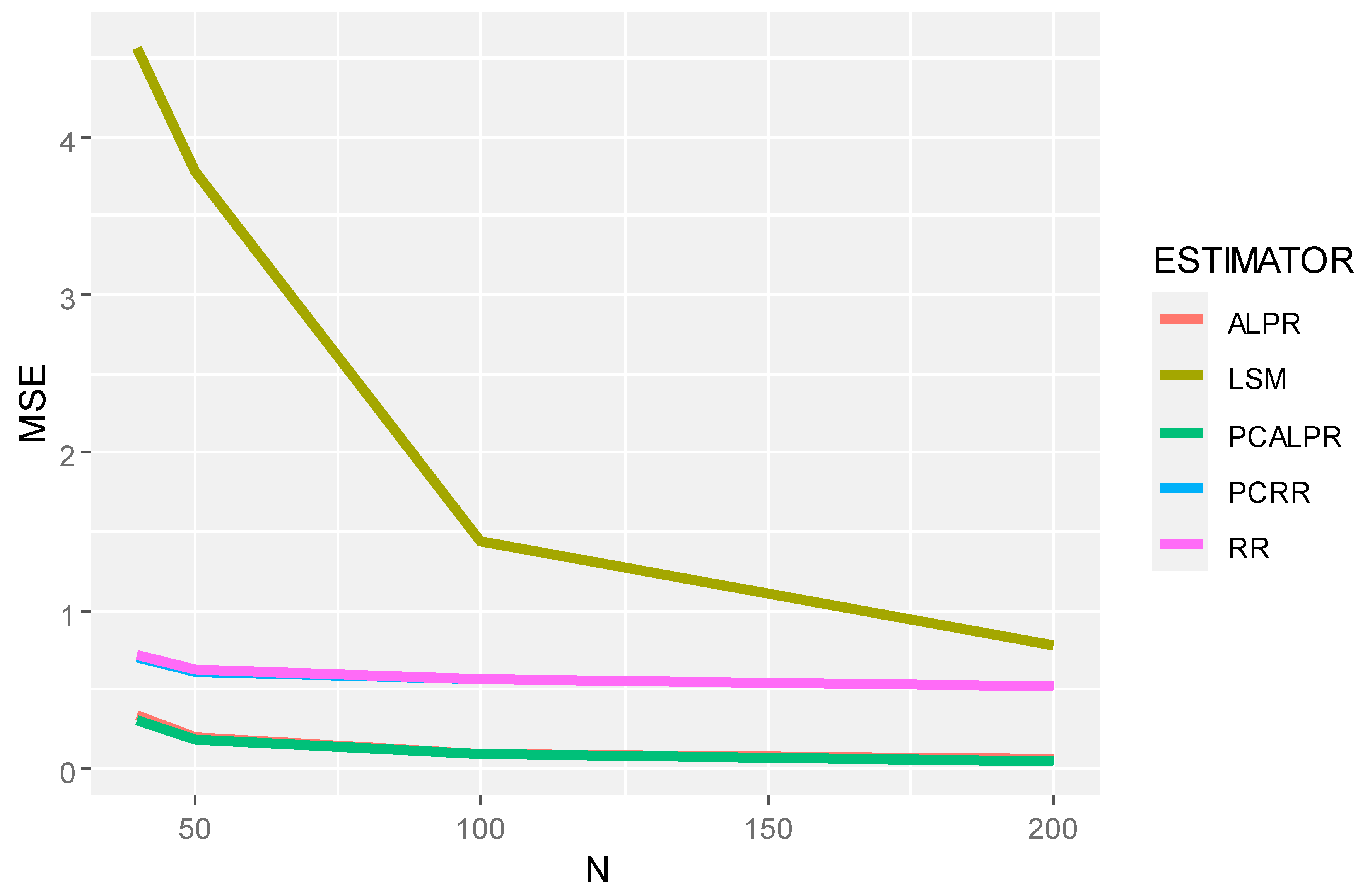
Least squares method (LSM), ridge regression (RR), principal components ridge regression (PCRR), average least squares method-centered penalized regression (ALPR), and principal component average least squares method-centered penalized regression (PCALPR).

. The results from the simulation study offer a comprehensive view of how different regression estimators perform under varying conditions of multicollinearity and noise levels. The comparison includes the traditional least squares method (LSM), ridge regression (RR), principal components ridge regression (PCRR), average least squares method-centered penalized regression (ALPR), and the novel principal component average least squares method-centered penalized regression (PCALPR). Under moderate to strong multicollinearity scenarios (ρ = 0.8 to ρ = 0.99), the PCALPR estimator consistently outperformed the other estimators in terms of mean squared error (MSE). This indicates a superior capability in accurately estimating the regression coefficients, which directly contributes to better model prediction accuracy. However, as the multicollinearity level is severe, i.e., when ρ = 0.999, other estimators compete favorably.

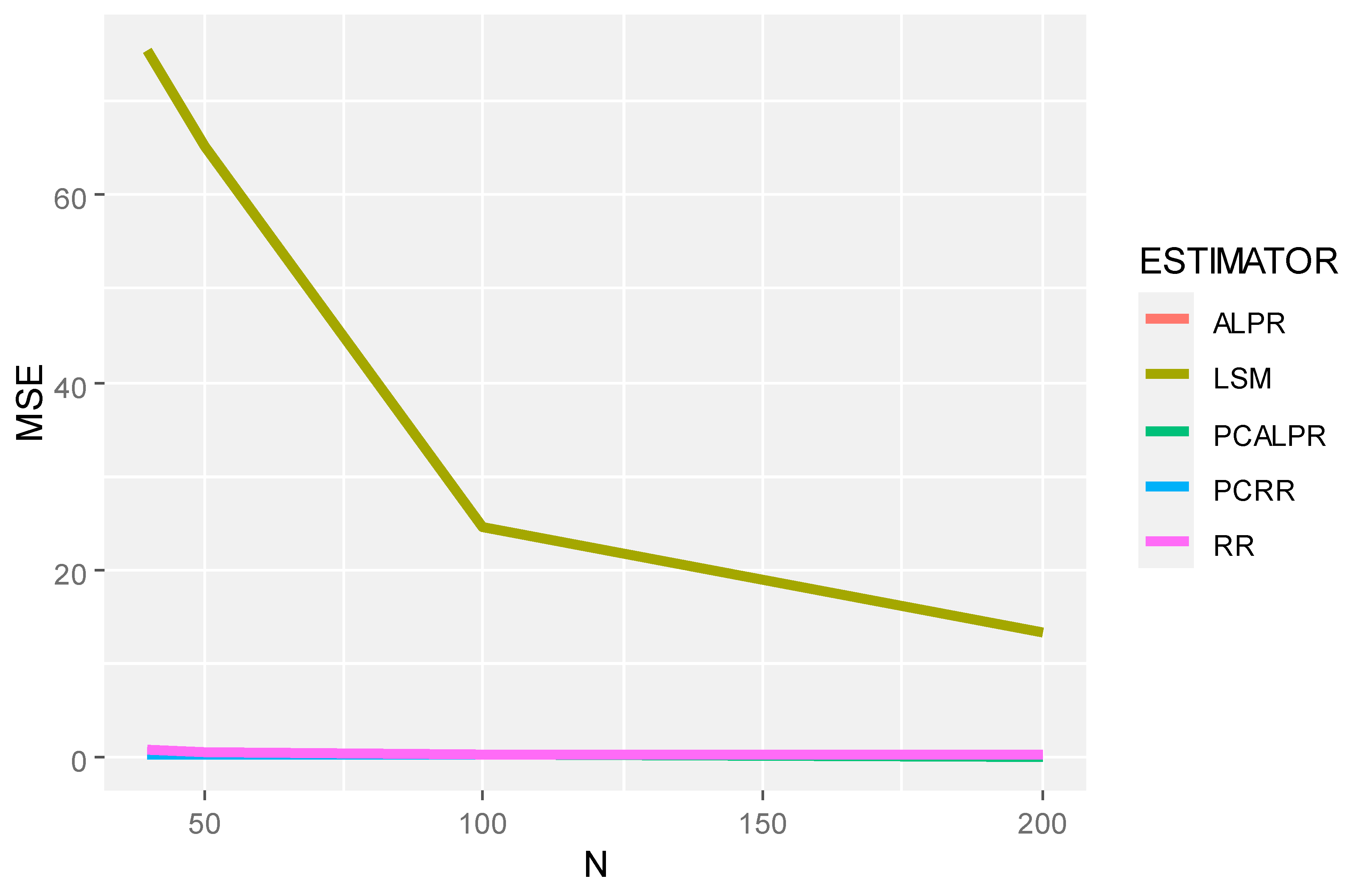
A key observation is a significant deterioration in the performance of the LSM as the level of multicollinearity increases, illustrating the well-known vulnerability of ordinary least squares to collinear predictors. This highlights the necessity for alternative estimation techniques in practical applications where predictors are often correlated to some degree.

Both RR and PCRR showed improvements over LSM, affirming the value of penalization and dimensionality reduction techniques in mitigating multicollinearity effects. However, the standout performance of ALPR and PCALPR underscores the effectiveness of centering the penalization around a more robust estimate than ordinary least squares, particularly under high multicollinearity.

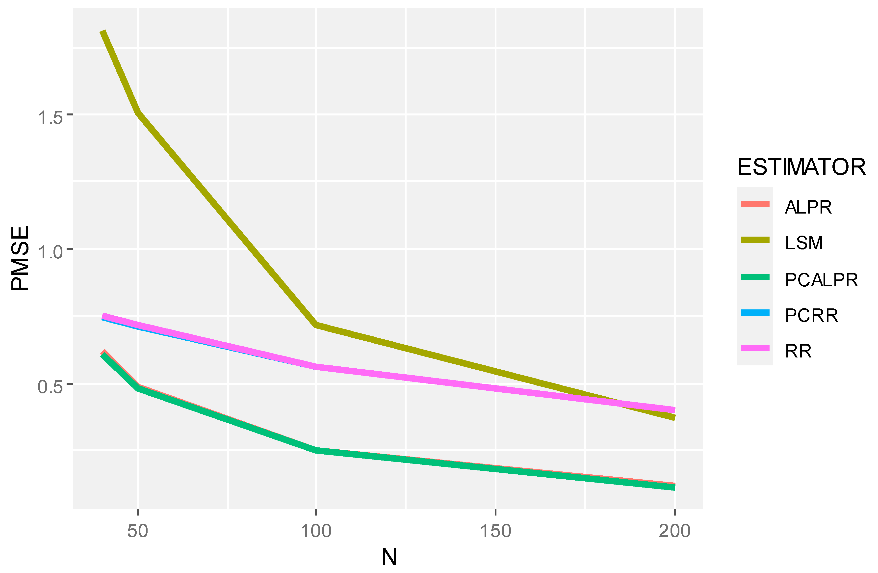
PCALPR’s edge over ALPR in almost all scenarios suggests that the integration of principal component analysis not only helps in addressing multicollinearity by reducing the dimensionality of the predictor space but also enhances the penalization strategy by focusing on the most informative components of the predictors.

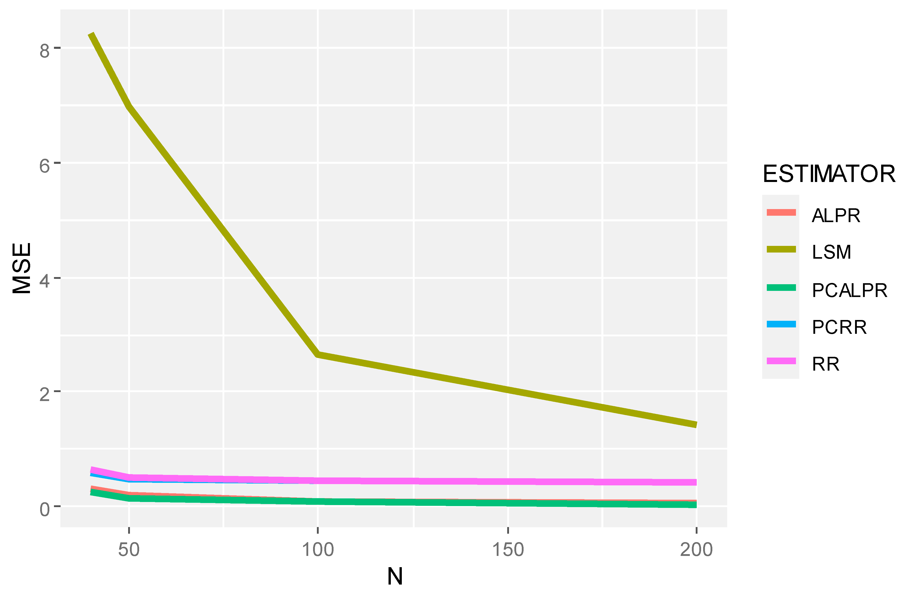
When examining the impact of different noise levels (σ² = 25 vs. σ² = 100), it is evident that all estimators perform worse as noise increases, as expected. However, the relative performance rankings remain roughly consistent, with PCALPR maintaining its superiority. This resilience to increased noise levels further supports the robustness of the proposed method. The mean squared error and prediction mean squared error decrease as the sample size increases, as demonstrated in Figure 1, Figure 2, Figure 3 and Figure 4.

The findings from this study suggest that PCALPR is a highly promising approach for handling multicollinearity in linear regression models, particularly in situations where predictors have high multicollinearity and when the model is subjected to significant noise. The method not only leverages the strengths of penalized regression techniques to reduce the bias introduced by multicollinearity but also capitalizes on the dimensionality reduction capability of principal component analysis to focus the model estimation on the most relevant information contained within the predictor variables.

4. Data Analysis

We evaluated the efficacy of the proposed and existing estimators by analyzing two real-life datasets.

4.1. Asphalt Binder Data

This dataset has been adopted in previous studies to analyze the impact of various chemical compositions on surface free energy [27,28]. The model formulation is as follows:

$$y_i={\beta }_0+{\beta }_1{x}_{i1}+\cdots +{\beta }_{12}{x}_{i12}+{\mathsf{\epsilon }}_i,i=1,\dots ,23$$

(28)

where $y_i$ denotes surface free energy; $x_{i1}$ through $x_{i12}$ correspond to saturates, aromatics, resins, asphaltenes, wax, carbon, hydrogen, oxygen, nitrogen, sulfur, nickel, and vanadium, respectively. We standardized the predictor variables to achieve a mean of zero and a variance of 1. We conducted the Ramsey RESET test to assess the linearity of the regression model. The test statistic yielded a value of RESET = 3.8065, p-value = 0.08283, with one degree of freedom in the numerator (df1) and nine degrees of freedom in the denominator (df2). The p-value of 0.08283 suggests there is no significant evidence to reject the null hypothesis of linearity at the conventional significance level of 0.05. Furthermore, the Breusch–Pagan test for heteroscedasticity (BP test) resulted in a statistic of BP = 9.9723, with 12 degrees of freedom and a p-value of 0.6184. This p-value indicates no evidence against the null hypothesis of homoscedasticity (constant variance) in the residuals. Therefore, there is no significant heteroscedasticity detected in the model. Considering both tests, while the Ramsey RESET test suggests strong evidence for linearity, the Breusch–Pagan test does not find evidence of heteroscedasticity.

The correlation plot (Figure 5) shows the presence of strong correlations among some predictor variables, such as between saturates, aromatics, resins, asphaltenes, etc. High correlation among predictors is a hallmark of multicollinearity, which complicates the estimation of regression coefficients because it becomes challenging to isolate the individual effect of each predictor on the response variable.

The VIF plot presented in Figure 6 quantitatively shows the degree of multicollinearity. A VIF value greater than 10 is often considered an indicator of severe multicollinearity, suggesting that the predictor variables are highly linearly related. This condition exacerbates the difficulty in obtaining reliable estimates of the regression coefficients because it inflates the variances in the coefficient estimates, making them less precise. In addition, the condition number is 52.37, revealing the presence of severe multicollinearity.

Table 5. Regression estimates for the Asphalt binder data.

Coefficients	${\widehat{\mathit{\alpha }}}_{\mathit{L}\mathit{S}\mathit{M}}$	${\widehat{\mathit{\alpha }}}_{\mathit{R}\mathit{R}}$	${\widehat{\mathit{\alpha }}}_{\mathit{P}\mathit{C}\mathit{R}\mathit{R}}$	${\widehat{\mathit{\alpha }}}_{\mathit{A}\mathit{L}\mathit{P}\mathit{R}}$	${\widehat{\mathit{\alpha }}}_{\mathit{P}\mathit{C}\mathit{A}\mathit{L}\mathit{P}\mathit{R}}$
Intercept	18.4213	18.2982	18.2982	17.7759	17.7771
${\mathit{x}}_{\mathit{i}\mathbf{1}}$	−0.9374	−0.9222	−0.9689	0.7659	0.6152
${\mathit{x}}_{\mathit{i}\mathbf{2}}$	1.0047	0.8501	0.1988	3.9515	3.4056
${\mathit{x}}_{\mathit{i}\mathbf{3}}$	0.5034	0.3194	0.9184	4.1772	4.7278
${\mathit{x}}_{\mathit{i}\mathbf{4}}$	−0.3170	−0.6309	−0.9350	1.6927	1.6568
${\mathit{x}}_{\mathit{i}\mathbf{5}}$	−1.4497	−1.4092	−0.6252	−0.7086	−0.0231
${\mathit{x}}_{\mathit{i}\mathbf{6}}$	0.6610	0.6166	0.5210	0.8970	0.9224
${\mathit{x}}_{\mathit{i}\mathbf{7}}$	0.9434	0.9178	0.3774	1.2513	0.7737
${\mathit{x}}_{\mathit{i}\mathbf{8}}$	1.1531	0.9678	0.5222	0.7573	0.6310
${\mathit{x}}_{\mathit{i}\mathbf{9}}$	−0.2055	0.0241	0.6825	0.9123	1.1603
${\mathit{x}}_{\mathit{i}\mathbf{10}}$	−1.2356	−1.0465	−0.5421	0.4754	0.6927
${\mathit{x}}_{\mathit{i}\mathbf{11}}$	1.0707	0.9054	−0.0403	1.1342	0.5469
${\mathit{x}}_{\mathit{i}\mathbf{12}}$	−0.6526	−0.5802	0.0206	−0.1788	0.2577
SMSE	131.4192	16.5916	16.2259	13.1748	11.4092

provides the regression estimates for different models: the least squares method (LSM), ridge regression (RR), principal component ridge regression (PCRR), average LSM-centered penalized regression (ALPR), and principal component average LSM-centered penalized regression (PCALPR). Each method adjusts the coefficients (β) differently based on their approach to handling multicollinearity. The intercept and coefficients vary across models, reflecting how each method compensates for the high correlation among predictors. For instance, ALPR and PCALPR provide coefficients that are significantly different from those of LSM, indicating a distinct approach to stabilizing the regression estimates in the presence of multicollinearity.

The standardized mean squared error (SMSE) is a measure of the accuracy of the estimator. Lower values indicate a better fit and more reliable estimates. From Table 5, it is evident that ALPR and PCALPR outperform the other methods, with PCALPR showing the lowest SMSE. This suggests that PCALPR, by incorporating both principal component analysis and average LSM-centered penalized regression, offers a more robust method for dealing with multicollinearity, providing more accurate and stable estimates of the regression coefficients. The coefficients estimated by ALPR and PCALPR indicate that these methods can identify and adjust for the influence of multicollinearity, leading to potentially more meaningful and interpretable results. For example, the positive coefficients for x₂, x₃, and x₇ in the ALPR and PCALPR models may suggest a strong positive relationship with the surface free energy, which was not as clearly indicated or was over-adjusted in the LSM and RR models.

4.2. Gasoline Mileage Data

The second dataset employed in this study was obtained from Montgomery et al. [3], comprising observations on gasoline mileage and eleven (11) predictors. We excluded variables three and eleven due to missing data in variable three and the structural form of variable eleven. Thus, we retained only nine of the features.

Table 6. Variable description.

Variable Name	Description
$x_{i1}$	Displacement (cubic inches)
$x_{i2}$	Horsepower (foot-pounds)
$x_{i4}$	Compression ratio
$x_{i5}$	Rear axle ratio
$x_{i6}$	Carburetor (barrels)
$x_{i7}$	Number of transmission speeds
$x_{i8}$	Overall length (inches)
$x_{i9}$	Width (inches)
$x_{i10}$	Weight (pounds)
$y$	Miles per gallon

provides a comprehensive description of each variable utilized in the regression model:

We standardized the predictor variables to achieve a mean of zero and a variance of 1. We conducted the Ramsey RESET test to assess the linearity of the regression model. The test statistic yielded a value of RESET = 3.7076, p-value = 0.07472, with 1 degree of freedom in the numerator (df1) and 14 degrees of freedom in the denominator (df2). The p-value of 0.07472 suggests there is no significant evidence to reject the null hypothesis of linearity at the conventional significance level of 0.05. Furthermore, the Breusch–Pagan test for heteroscedasticity (BP test) resulted in a statistic of BP = 3.6087, with nine degrees of freedom and a p-value of 0.9352. This p-value indicates no evidence against the null hypothesis of homoscedasticity (constant variance) in the residuals. Therefore, there is no significant heteroscedasticity detected in the model. Considering both tests, while the Ramsey RESET test suggests strong evidence for linearity, the Breusch–Pagan test does not find evidence of heteroscedasticity. The correlation plot presented in Figure 7 helps to identify the strength and direction of linear relationships between predictor variables. High correlation coefficients between pairs of predictors suggest a strong linear relationship, potentially indicating multicollinearity. Multicollinearity complicates the interpretation of individual predictors’ effects on the response variable due to shared variance among predictors. The VIF quantifies how much the variance of an estimated regression coefficient increases if the predictors are correlated. If no factors are correlated, the VIF equals 1. Generally, a VIF above 5–10 indicates significant multicollinearity requiring attention. In the context of Gasoline Mileage data, the presence of multicollinearity (as indicated by the VIF plot in Figure 8) suggests that some of the predictors share a significant amount of information, which could distort the regression coefficients if not properly addressed. In addition, the condition number is 26.80, revealing the presence of moderate multicollinearity.

The regression estimates across different methods presented in

Table 7. Regression estimates for the Gasoline Mileage data.

Coefficients	${\widehat{\mathit{\alpha }}}_{\mathit{L}\mathit{S}\mathit{M}}$	${\widehat{\mathit{\alpha }}}_{\mathit{R}\mathit{R}}$	${\widehat{\mathit{\alpha }}}_{\mathit{P}\mathit{C}\mathit{R}\mathit{R}}$	${\widehat{\mathit{\alpha }}}_{\mathit{A}\mathit{L}\mathit{P}\mathit{R}}$	${\widehat{\mathit{\alpha }}}_{\mathit{P}\mathit{C}\mathit{A}\mathit{L}\mathit{P}\mathit{R}}$
Intercept	20.6208	19.3242	0.0000	13.9381	−0.3106
${\mathit{x}}_{\mathit{i}\mathbf{1}}$	−6.0835	−2.9430	−0.9192	−1.2406	−1.1774
${\mathit{x}}_{\mathit{i}\mathbf{2}}$	2.5176	−0.6611	−0.8649	−0.8659	−0.9807
${\mathit{x}}_{\mathit{i}\mathbf{4}}$	0.9377	0.6267	0.4281	0.5940	0.1501
${\mathit{x}}_{\mathit{i}\mathbf{5}}$	0.9549	0.5652	0.6963	0.6008	0.2435
${\mathit{x}}_{\mathit{i}\mathbf{6}}$	0.6851	0.2456	−0.5545	−0.3273	−0.6128
${\mathit{x}}_{\mathit{i}\mathbf{7}}$	−1.4518	0.0294	0.7797	0.6480	0.1987
${\mathit{x}}_{\mathit{i}\mathbf{8}}$	4.1051	0.9788	−0.8500	−0.2911	−0.9909
${\mathit{x}}_{\mathit{i}\mathbf{9}}$	0.6992	−0.5416	−0.8113	−0.6839	−1.0333
${\mathit{x}}_{\mathit{i}\mathbf{10}}$	−7.1948	−2.1462	−0.9077	−1.0316	−1.0077
SMSE	782.956	117.959	70.568	199.089	27.276

(least squares method (LSM), ridge regression (RR), principal component ridge regression (PCRR), average LSM-centered penalized regression (ALPR), and principal component average LSM-centered penalized regression (PCALPR)) show how each predictor variable is estimated to impact the mileage, adjusting for the presence of other variables in the model. Each method handles multicollinearity differently, leading to variations in coefficient estimates. Each coefficient represents the change in the mileage associated with a one-unit change in the predictor variable, holding all other predictors constant. The variation in coefficient estimates across different methods reflects each method’s approach to managing multicollinearity and optimizing the model for prediction accuracy. Differences in coefficient estimates across methods highlight the impact of multicollinearity and the effectiveness of each method in addressing it. For example, penalized methods like RR, ALPR, and PCALPR may shrink some coefficients towards zero more than others, reflecting their relative importance in the presence of multicollinearity. The SMSE values across different estimation methods in Table 7 provide insight into each model’s prediction accuracy. Lower SMSE values indicate better model performance in terms of accurately predicting the softening point from the given predictors. The variation in SMSE values reflects the trade-off between bias and variance introduced by each regression method, with penalized methods typically offering a more balanced approach to minimize prediction error. The principal component average LSM-centered penalized regression (PCALPR) outperforms the others in terms of the SMSE criterion, making it the most accurate model for predicting gasoline mileage from the given predictors in the presence of multicollinearity. This suggests that the combination of principal component regression (PCR) with average LSM-centered penalized regression (ALPR) to reduce dimensionality and multicollinearity provides a robust estimation.

5. Conclusions

This work focused on estimating the regression parameters for a predictive linear model when there is multicollinearity among the regressors. We utilized the optimal shrinkage method, ALPR, developed by Wang et al. [14] and combined it with the principal component (PC) technique. We determined the property of the proposed PCALPR and compared using the mean squared error (MSE) with other estimators such as the least squared method, PC regression, ridge regression, and ALPR using numerical analysis. Comprehensive numerical evaluations demonstrated that our suggested estimator dominates others via the MSE across various degrees of multicollinearity. We observed that the prediction accuracy of the new estimator closely matches that of the ALPR. The effectiveness of the PCALPR in severe multicollinear predictive modelling was demonstrated through data analysis, showing improved prediction accuracy.

References

1. Gunst, R.F. Regression analysis with multicollinear predictor variables: Definition, detection, and effects. Commun. Stat. Theory Methods 1983, 12, 2217–2260. [Google Scholar] [CrossRef]
2. Weisberg, S. Applied Regression Analysis; Wiley: Hoboken, NJ, USA, 1985. [Google Scholar]
3. Montgomery, D.C.; Peck, A.E.; Vining, G.G. Introduction to Linear Regression Analysis, 5th ed.; John Wiley & Sons, Inc.: Hoboken, NJ, USA, 2012. [Google Scholar]
4. Dawoud, I.; Kibria, G. A New biased estimator to combat the multicollinearity of the Gaussian linear regression model. Stats 2020, 3, 526–541. [Google Scholar] [CrossRef]
5. James, G.; Witten, D.; Hastie, T.; Tibshirani, R. An Introduction to Statistical Learning; Springer: Berlin/Heidelberg, Germany, 2013. [Google Scholar]
6. Næs, T.; Indahl, U. A unified description of classical classification methods for multicollinear data. J. Chemom. 1998, 12, 205–220. [Google Scholar] [CrossRef]
7. Hoerl, A.E.; Kennard, R.W. Ridge regression: Biased estimation for nonorthogonal problems. Technometrics 1970, 12, 55–67. [Google Scholar] [CrossRef]
8. Liu, K. A new class of biased estimate in linear regression. Commun. Stat. Theory Methods 1993, 22, 393–402. [Google Scholar]
9. Kibria, B.M.G.; Lukman, A.F. A new ridge-type estimator for the linear regression model: Simulations and applications. Scientifica 2020, 2020, 9758378. [Google Scholar] [CrossRef] [PubMed]
10. Owolabi, A.T.; Ayinde, K.; Alabi, O.O. A new ridge-type estimator for the linear regression model with correlated regressors. Concurr. Comput. Pract. Exp. 2022, 34, e6933. [Google Scholar] [CrossRef]
11. Lukman, A.F.; Ayinde, K.; Binuomote, S.; Clement, O.A. Modified ridge-type estimator to combat multicollinearity: Application to chemical data. J. Chemom. 2019, 33, e3125. [Google Scholar] [CrossRef]
12. Qasim, M.; Månsson, K.; Sjölander, P.; Kibria, B.G. A new class of efficient and debiased two-step shrinkage estimators: Method and application. J. Appl. Stat. 2021, 49, 4181–4205. [Google Scholar] [CrossRef]
13. Stein, C.M. Multiple Regression Contributions to Probability and Statistics. Essays in Honor of Harold Hoteling; Stanford University Press: Palo Alto, CA, USA, 1960. [Google Scholar]
14. Wang, W.; Li, L.; Li, S.; Yin, F.; Liao, F.; Zhang, T.; Li, X.; Xiao, X.; Ma, Y. Average ordinary least squares-centered penalized regression: A more efficient way to address multicollinearity than ridge regression. Stat. Neerl. 2022, 76, 347–368. [Google Scholar] [CrossRef]
15. Baye, R.; Parker, F. Combining ridge and principal component regression: A money demand illustration. Commun. Stat. Theory Methods 1984, 13, 197–205. [Google Scholar] [CrossRef]
16. Farghali, R.A.; Lukman, A.F.; Ogunleye, A. Enhancing model predictions through the fusion of Stein estimator and principal component regression. J. Stat. Comput. Simul. 2024. [Google Scholar] [CrossRef]
17. Davino, C.; Romano, R.; Vistocco, D. Handling multicollinearity in quantile regression through the use of principal component regression. METRON 2022, 80, 153–174. [Google Scholar] [CrossRef]
18. Kaçıranlar, S.; Sakallıoğlu, S. Combining the Liu estimator and the principal component regression estimator. Commun. Stat. Theory Methods 2001, 30, 2699–2705. [Google Scholar] [CrossRef]
19. Chang, X.; Yang, H. Combining two-parameter and principal component regression estimators. Stat. Pap. 2012, 53, 549–562. [Google Scholar] [CrossRef]
20. Lukman, A.F.; Ayinde, K.; Oludoun, O.; Onate, C.A. Combining modified ridge-type and principal component regression estimators. Sci. Afr. 2020, 9, e00536. [Google Scholar] [CrossRef]
21. Vajargah, K.F. Comparing ridge regression and principal components regression by monte carlo simulation based on MSE. J. Comput. Sci. Comput. Math. 2013, 3, 25–29. [Google Scholar] [CrossRef]
22. Wu, J. On the performance of principal component Liu-type estimator under the mean square error criterion. J. Appl. Math. 2013, 2013, 858794. [Google Scholar] [CrossRef]
23. Cliff, N. The eigenvalues-greater-than-one rule and the reliability of components. Psychol. Bull. 1988, 103, 276–279. [Google Scholar] [CrossRef]
24. Hoerl, A.E.; Kannard, R.W.; Baldwin, K.F. Ridge regression: Some simulations. Commun. Stat. 1975, 4, 105–123. [Google Scholar] [CrossRef]
25. Li, S.; Wang, W.; Yao, M.; Wang, J.; Du, Q.; Li, X.; Tian, X.; Zeng, J.; Deng, Y.; Zhang, T.; et al. Poisson Average Maximum Likelihood-Centered Penalized Estimator: A New Estimator to Better Address Multicollinearity in Poisson Regression. Stat. Neerl. 2022, 78, 208–227. [Google Scholar] [CrossRef]
26. Kaiser, H.F. The application of electronic computers to factor analysis. Educ. Psychol. Meas. 1960, 20, 141–151. [Google Scholar] [CrossRef]
27. Lukman, A.F.; Allohibi, J.; Jegede, S.L.; Adewuyi, E.T.; Oke, S.; Alharbi, A.A. Kibria–Lukman-Type Estimator for Regularization and Variable Selection with Application to Cancer Data. Mathematics 2023, 11, 4795. [Google Scholar] [CrossRef]
28. Arashi, M.; Asar, Y.; Yüzbaşı, B. SLASSO: A scaled LASSO for multicollinear situations. J. Stat. Comput. Simul. 2021, 91, 3170–3183. [Google Scholar] [CrossRef]
Figure 1. Estimated PMSE by sample size when ρ = 0.8, p = 3, and σ = 5.
Symmetry 16 00469 g001
Figure 2. Estimated MSE by sample size when ρ = 0.9, p = 3, and σ = 5.
Symmetry 16 00469 g002
Figure 3. Estimated MSE by sample size when ρ = 0.99, p = 3, and σ = 5.
Symmetry 16 00469 g003
Figure 4. Estimated PMSE by sample size when ρ = 0.99, p = 3, and σ   = 5.
Symmetry 16 00469 g004
Figure 5. Correlation heatmap for Asphalt Binder dataset.
Symmetry 16 00469 g005
Figure 6. Variance inflation plot for Asphalt Binder dataset.
Symmetry 16 00469 g006
Figure 7. Correlation heatmap for Gasoline Mileage dataset.
Symmetry 16 00469 g007
Figure 8. Variance inflation plot for Gasoline Mileage dataset.
Symmetry 16 00469 g008