Method PPC for Precise Piecewise Correlation after Histogram Segmentation

Abstract

Correlation, functioning as a symmetric relation, is very powerful indicator of the mutual association between two attributes. The problem of weak correlation indicates a lack of linearity in the observed range. This paper presents the precise piecewise correlation method, which overcomes the problem by determining the segments where the linear association will be present. The determination was achieved using the histogram segmentation method. The conditions of the application and analysis of the method are presented, as well as the application of the method to the representative datasets. The obtained results confirm the existence of stronger linear associations on the segments. Detected correlations reveal the strength and nature of the symmetric association between two attributes on each of the separated segments.

1. Introduction

This paper emphasizes the importance of piecewise correlation and presents a new method for determining correlation based on histogram segmentation. It happens that two considered attributes are weakly correlated in the whole range but there exist notably stronger correlation if observing subranges. Subranges are predefined if there exists some classification within one of the attributes. But, if there is lack of any classification, the novel method imposes piecewise correlation determined via histogram segmentation produced by the intersections of kernel density estimations [1]. Piecewise correlation is feasible if at least one of the attributes has a multimodal histogram.

Behind the development of the method is an idea that was first applied in [2], where the analyzed data had a low correlation on the entire dataset. By applying the histogram segmentation design [3], correlation by segments was achieved, and noticeably higher values were obtained. A connection between the choice of multimodal histogram and gain ratio was observed. It is important to emphasize that correlation is a completely symmetric and mutual feature of two attributes.

For the initial promotion of the novel method, a representative Iris dataset was used [4]. It contains four attributes to be compared and correlated. Each considered attribute has a finite set of values and, furthermore, has a corresponding empirical distribution and histogram, with an associated random variable. The initial correlation between the attributes will be computed and used for comparison with piecewise correlations obtained by the proposed method.

Additionally, the proposed PPC method was applied to three more datasets. The Dryad dataset [5] has been segmented by histograms of real distances for horizontal and vertical nodes, which enabled significant correlations between attributes. The Pima Indians Diabetes Database [6] is an example of one of the weaker achievements of the PPC method, with appropriate explanation. The Glass dataset [7] represents a case where the PPC method cannot be applied.

The method implies determination of gain ratio and segmented histogram for each attribute. The segmentation of the attribute with the highest gain ratio will be extended to the entire data, i.e., on all the attributes. After the global segmentation, the attributes will be correlated again, separately within each segment. The final correlation will be observed piecewise and, therefore, more accurate than the initial correlation. The proposed procedure justifies the name of the method that will be exposed, Precise Piecewise Correlation (PPC), after histogram segmentation.

The structure of the paper is as follows: The Section 2 presents the used related methods. It emphasizes correlation as the main subject of research. Next, the segmentation histogram and the related kernel density estimation function are presented. The last method used concerns entropy and its reduction measured by the term gain ratio. The Section 3 details the new PPC method, precise piecewise correlation, after histogram segmentation. In Section 4, the method is applied to the Iris dataset, Dryad dataset and Diabetes Database. In addition, the Glass dataset, where the method is not applicable, is considered.

The Section 5 contains a discussion of the results obtained by the PPC method applied to the Iris dataset and a comparison with the initial correlation, but also with the correlation based on the flower-type clustering. At the end of the discussion, the case where the method is not applicable is considered. The conclusion ends this paper.

2. Related Methods

2.1. Correlation

Correlation is a widely used statistical measure expressing the linear dependency of two variables. It does not inform on cause and effect, but only on the intensity of the connection. The Pearson correlation coefficient [8] is a relative quantity of the correlation that ranges between −1 and +1. The coefficient close to zero reflects a lack of correlation, while its closeness to ±1 means strong linear dependency. A positive correlation indicates that values of both variables tend to increase together, while the negative one specifies that two variables have opposite tendencies. The Pearson correlation coefficient of the two variables X and Y can be determined using the following formula:

$$corr\left(X,Y\right)=\frac{E\left(\left(X-E\left(X\right)\right)\left(Y-E\left(Y\right)\right)\right)}{{\sigma }_X{\sigma }_Y}$$

(1)

where E is the expectation operator and σ is the standard deviation. A comprehensive overview of various types of correlation and their interpretations can be found in [9,10]. Due to the symmetry of correlation, variables can be arbitrarily designated as independent or dependent. Correlation is visualized on scatterplots by interpolating a straight line between the points. Often a line is not a good enough model for points, e.g., if the points are placed near to a parabolic curve. By splitting the points into two or more regions, the correlation can be observed separately within each region, and the corresponding correlation coefficients will be noticeably higher. We will develop this type of correlation and call it the precise piecewise correlation. It should be emphasized that a segmented correlation, although the term sounds similar to the piecewise correlation, is a type of autocorrelation and a common tool in algorithms that extract a target signal in seismic communication [11].

In this research correlation will be determined for attributes from the database.

2.2. Histogram Segmentation and Kernel Density Estimation

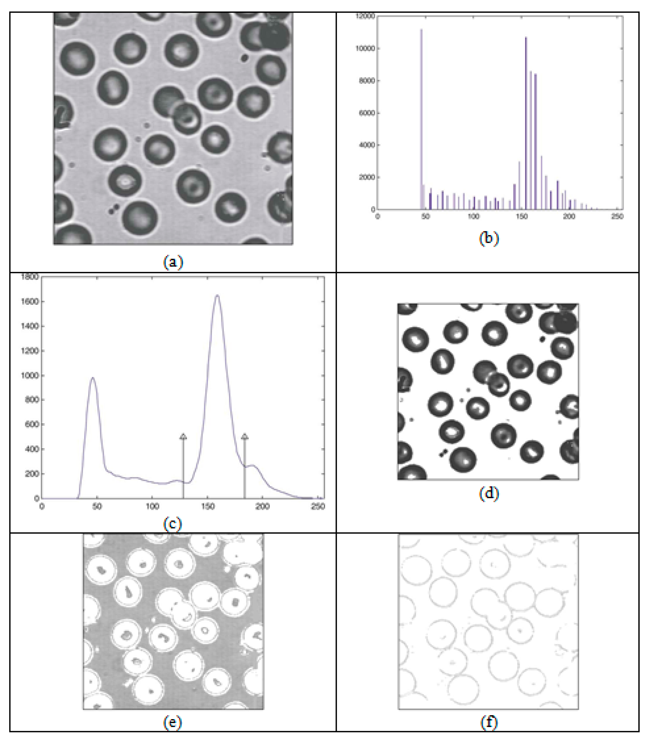
Histogram segmentation was initially conducted for needs within image processing, but it was later used in any data analysis [12]. Investigations concerned with image segmentation based on segmentation of the histogram had a major influence on this research. In [13], an analysis of the blood image was carried out, with the histogram having two thresholds: Figure 1 shows a blood image (a), a histogram (b), a smooth curve obtained by a histogram (c), and images obtained on the basis of histogram segmentation. Based on the first part of the segmentation, a blood cell image (d) was obtained, based on the second part of the segmentation, a blood plasma image (e) was obtained and based on the third part of the segmentation, and image of membrane cells (f) was obtained. The used sample has multimodal distribution with only three clusters, but it well reflects the multilevel thresholding technic presented in [13], where each cluster is analyzed by its deterministic parameters (mean, variance and probability). Based on the parameters, the thresholds are extracted.

If the segmentation of image histograms can extract clusters (see Figure 1d–f), then what kind of connection exists between the segmentation of the data histogram and data clusters? The basic concept of this paper will be generalized to any data.

On the other side, investigations of image segmentations have confirmed that image segmentation thresholds are located in the valleys between histogram peaks. Thus, histogram thresholding is the segmentation technique that looks for the peaks and valleys of the histogram [14]. The threshold selection of image histogram deals with clustering [15,16], hierarchical clustering (image segmentation by histogram thresholding using hierarchical cluster analysis) [17], classical rough sets [18], rough sets combined with other techniques [19], and deep learning [20].

In the threshold selection analysis, unimodal and multimodal histograms are of the interest for statistical and practical reasons [21].

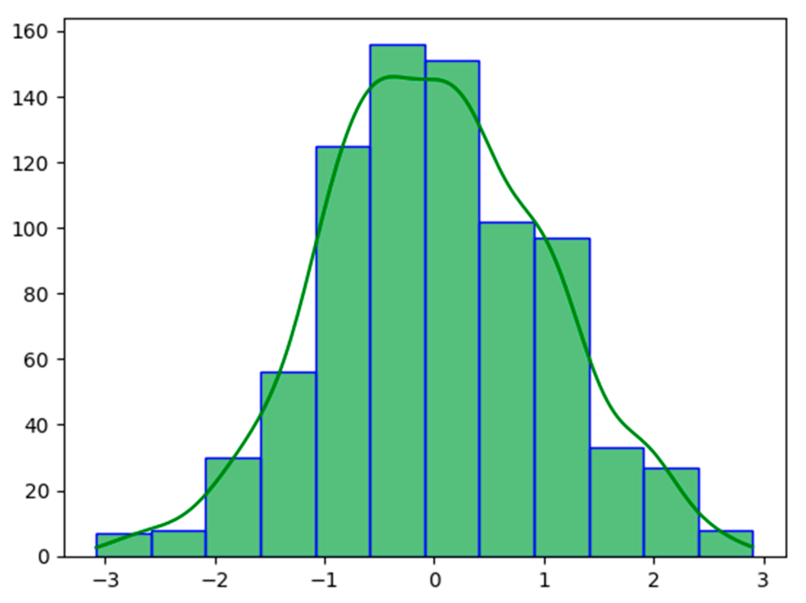
Kernel density estimation (KDE) is a technique for the estimation of the probability density function that is a must-have enabling the user to better analyze the studied probability distribution than when using a traditional histogram. Unlike the histogram, the kernel technique produces a smooth estimate of the probability density function (pdf), using all sample points’ locations and more convincingly suggesting multimodality [22].

The KDE function has two determining parameters. The kernel function is the first one, and it is commonly chosen to be Gaussian normal distribution. The second one is bandwidth, a real positive number that defines the smoothness of the density plot. The parameters must be carefully chosen; otherwise, they may lead to undesired transformations in the density plot [23].

An example of a histogram and associated kernel density estimation function are presented in Figure 2.

2.3. Entropy, Information Gain, and Gain Ratio

Entropy and Information Gain are closely related and both have similar purposes: to assess the quality of statistical models and determine the best approach in data analysis processes. Entropy is associated with a random variable as a measure of the uncertainty, while Information Gain is a measure of the decrease in uncertainty resulting by the collection of additional information from data [24,25].

Entropy is the measure of disorder [26], and it is calculated by measuring the amount of uncertainty in a given set of data. It is determined by the probability distribution of the data. If a set of data is uniformly distributed, the Entropy will be high, meaning that the data points are highly uncertain, and if the data points are clustered, the Entropy will be low, meaning that the data points are more certain. So, as Entropy is uncertainty in the data, the more “randomness”, the higher the Entropy will be. By adding new data, the Entropy is reduced because the uncertainty associated with data decreases.

On the other hand, Information Gain measures how well a dataset can be modeled and how accurately the data can be predicted. Information Gain uses Entropy to make decisions. If the Entropy is less, information will be more. Information Gain is used in decision trees and random forest to decide the best split. These concepts are obviously connected because the more the Entropy is removed, the greater the Information Gain, and the higher the Information Gain, the better the split. Information Gain can also be seen as the difference between the Entropy before and after the decision. Entropy is minimal (0) when all examples are positive or negative, and maximal (1) when half of the examples are positive and half of the examples are negative.

The Shenon Entropy of an attribute (variable) A is determined by its distribution law (a_k, p_k), k = 1, …, n, in the following way:

$$\mathrm{H}\left(\mathrm{A}\right)=-{\displaystyle {\sum }_{\mathrm{k}=1}^{\mathrm{n}}{\mathrm{p}}_{\mathrm{k}}\cdot {\log }_2}{\mathrm{p}}_{\mathrm{k}}$$

(2)

where a_k represents the values or value intervals of the attribute A and p_k represents their relative frequencies. Thus, the Entropy H(A) reflects the disorder among the data on the attribute A. Further, a metric is needed to measure the reduction in this disorder in the considered attribute after obtaining additional information, usually about some clustering within the attribute. This is where Information Gain comes in. Information gain IG(A) quantifies the reduction in Entropy (uncertainty) through the acquisition of knowledge about the attribute achieved by MDL algorithm discretization [27]. Information Gain is used in decision tree learning algorithms in order to measure the relative Entropy of an attribute with respect to the target class. When building a decision tree, it is used to identify the most important attribute and decide which attribute should be placed at the root of the tree.

Gain Ratio is an alternative complement to Information Gain, and it is also used to select the attribute for splitting in a decision tree. Gain Ratio use Information Gain, so they have the following formulas:

$$\mathrm{InfoGain}(\mathrm{class},\mathrm{A})=\mathrm{H}\left(\mathrm{class}\right)-\mathrm{H}\left(\mathrm{class}\right|\mathrm{A})$$

(3)

$$\mathrm{GainRatio}(\mathrm{class},\mathrm{A})=\left(\mathrm{H}\right(\mathrm{class})-\mathrm{H}(\mathrm{class}\left|\mathrm{A}\right))/\mathrm{H}(\mathrm{A})$$

(4)

where H is Entropy and A is attribute.

The Gain Ratio can also be used to identify which attributes should be used at each level of the decision tree. It helps to create more accurate predictions or decisions. If two attributes with different numbers of possible values have the same Entropy, Information Gain cannot differentiate them. In the same situation, the Gain Ratio will favor attribute with less possible values. The Gain Ratio is a relative measure of the Entropy (it is a number in the interval [0, 1]) which facilitates the comparation of various attributes.

In this research the Gain Ratio will be used to distinguish the most valuable attribute.

3. Method PPC

This method enables piecewise correlation within a dataset without imposed clustering, based on the segmentation of the multimodal histogram of an attribute. Only datasets containing measured values at all attributes are suitable for this method.

The method is intended for working with tabular data that are organized by attributes. Histogram segmentation and Gain Ratio must be determined for each attribute. The first criterion checks whether the attribute has a multimodal histogram. In case where there are no attributes with a multimodal histogram, the method terminates. The highest gain ratio is the criterion for one attribute extraction. The histogram segmentation thresholds of the extracted attribute become the thresholds of the entire dataset and produce clusters for the piecewise correlation.

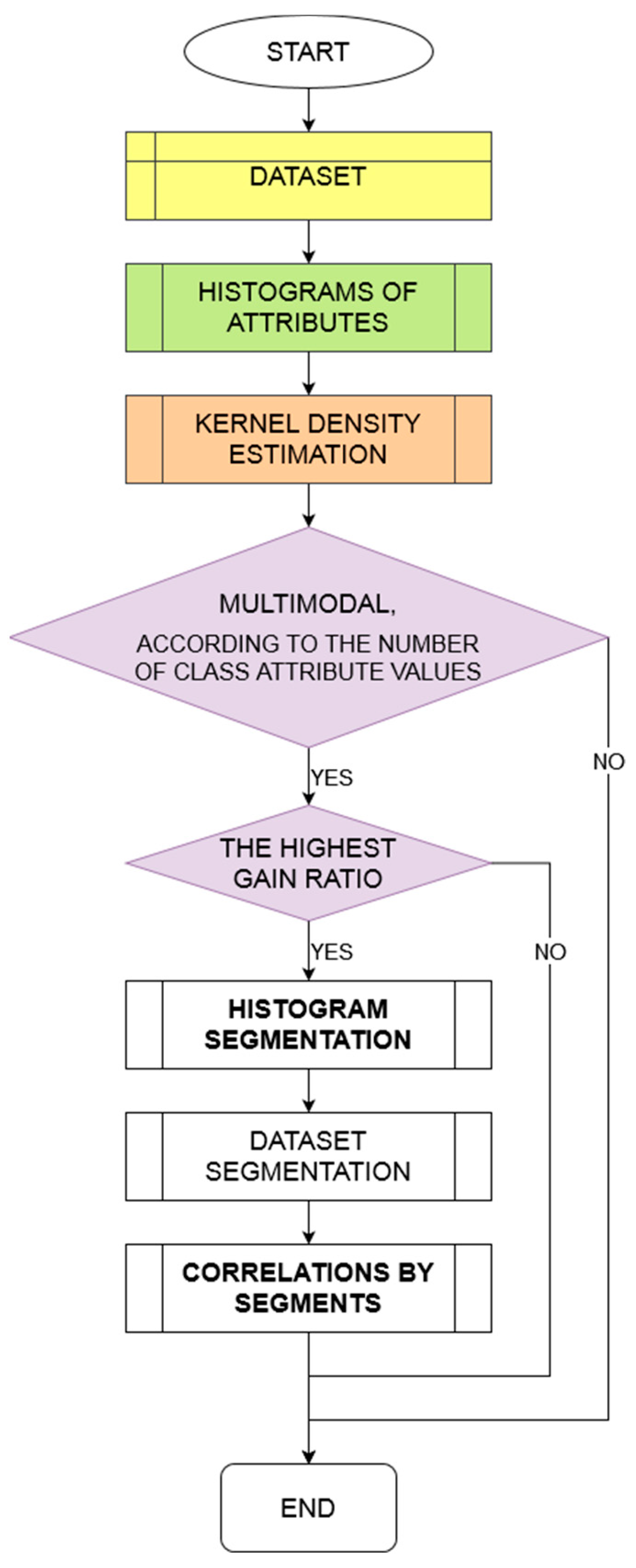
The individual steps of implementing the method are as follows (see Figure 3):

• Histograms of attributes-At the very beginning, a histogram for each of the attributes must be created. These histograms are necessary inputs for the KDE technique.
• KDE function-By using the Gaussian normal distribution as the kernel and selecting a sufficiently small positive bandwidth to produce a minimum, the KDE technique establishes histogram thresholds for each of the attributes. Furthermore, it verifies the multimodality property of the attributes, according to the number of class attribute values.
• Gain Ratio-To ascertain the attribute with the highest Gain Ratio, it is essential to calculate the Gain Ratio of each attribute by using (4).
• Histogram segmentation-Only the segmentation of the attribute with the highest gain ratio will be retained. The segmentations of the other attributes are discarded.
• Segmentation of the entire dataset-The segmentation of the attribute with the highest gain ratio determines the thresholds that will be used to segment the database. The entire dataset is then divided based on the instances highlighted by these thresholds.
• Correlations by segments-The correlations for all pairs of attributes are computed separately within each segment of the database.

4. PPC Method Application

The PPC method was applied to two selected datasets chosen to have different histogram distributions. Specifically, the Iris, the Dryad, the Pima Indian Diabetes, and Glass datasets were considered.

4.1. Application on the Iris Dataset

The PPC method was applied to the representative iris dataset [4]. The dataset contains 3 classes of 50 instances each, where each class referred to a type of iris plant. The attribute information was as follows:

• a1. sepal length in cm
• a2. sepal width in cm
• a3. petal length in cm
• a4. petal width in cm
• class:

  --

  Iris Setosa

  --

  Iris Versicolor

  --

  Iris Virginica

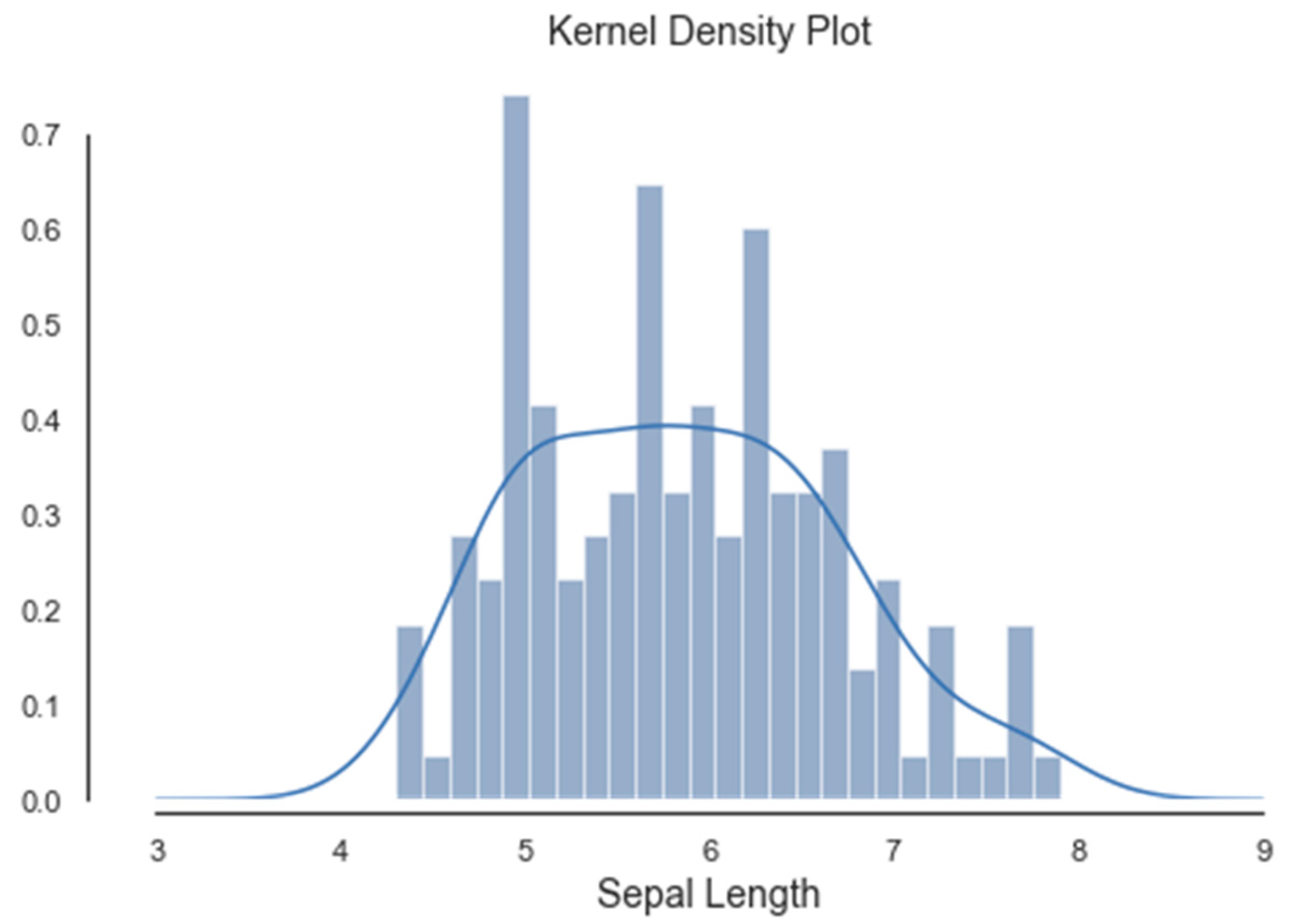
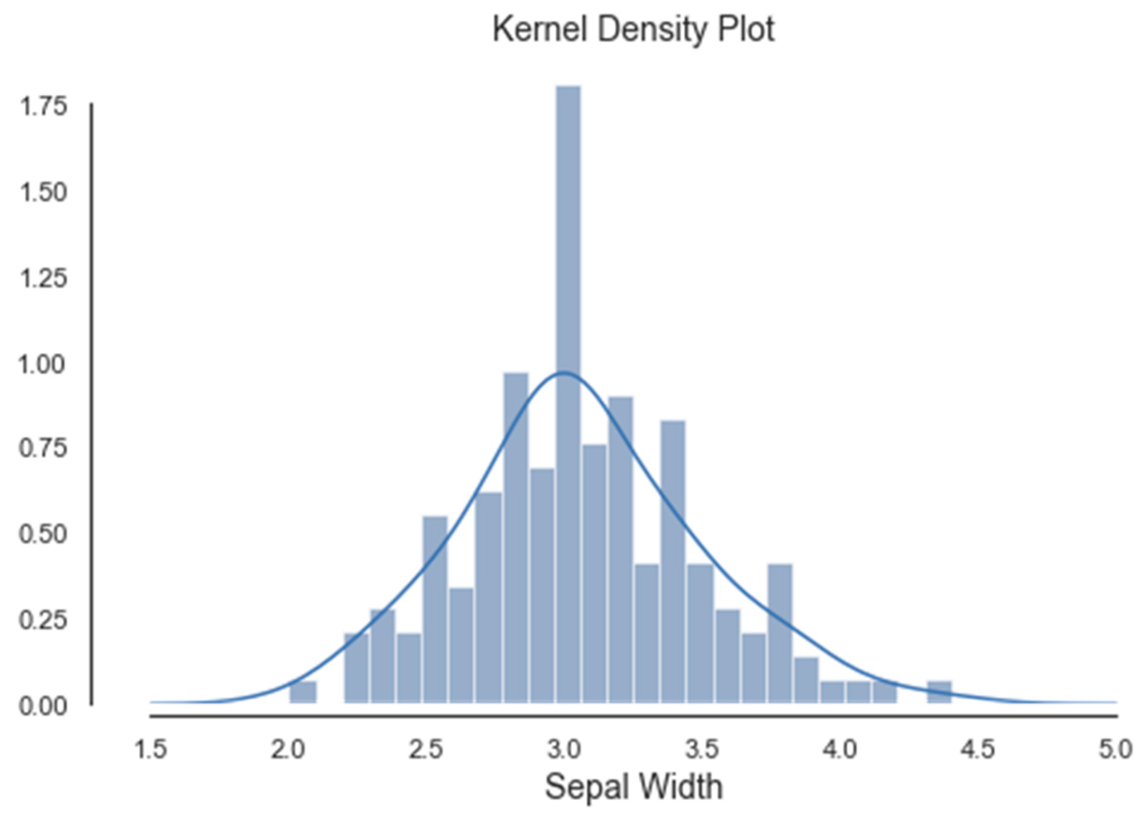
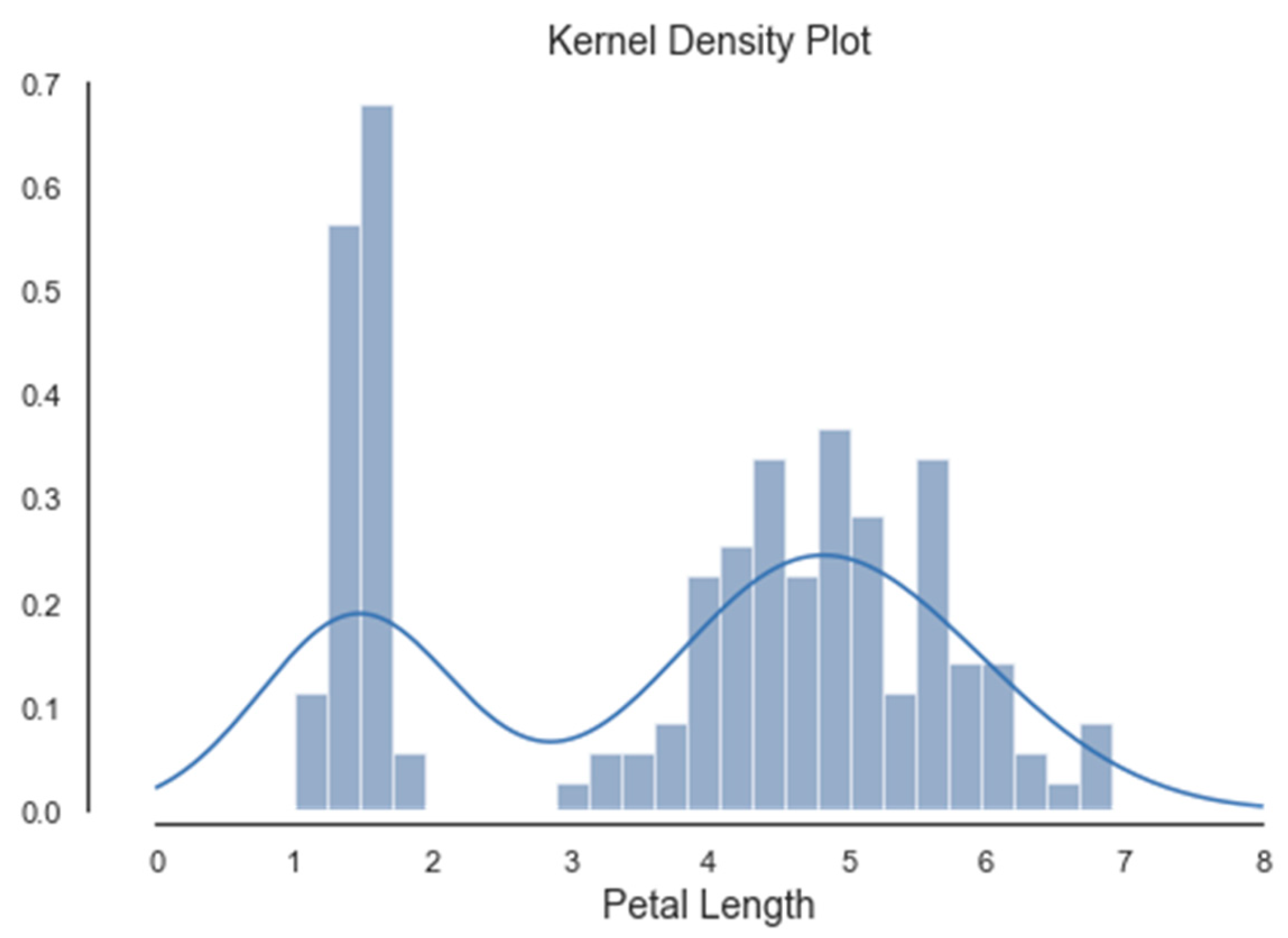
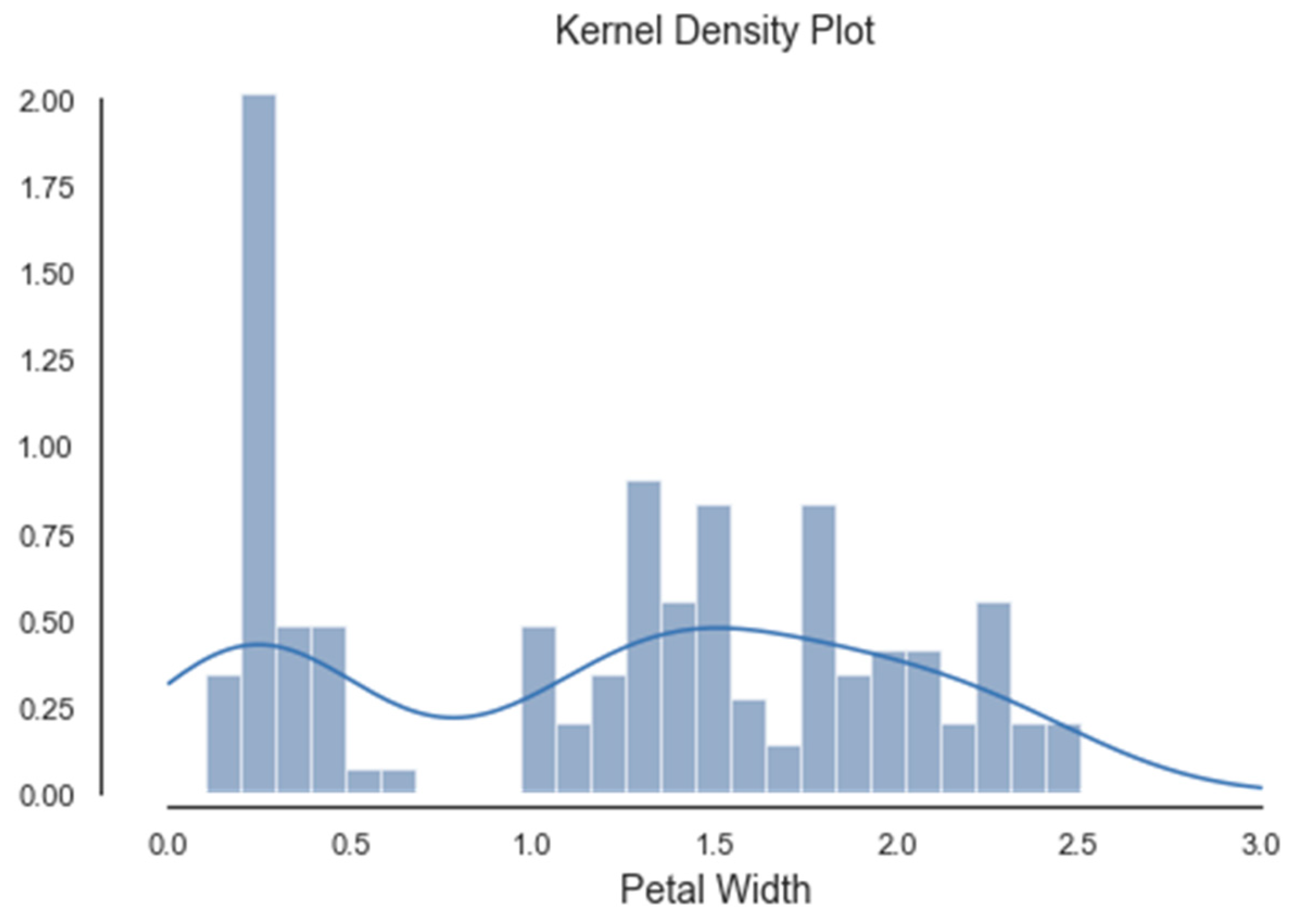
Histograms of the first four attributes are generated and shown with associated KDE functions in Figure 4, Figure 5, Figure 6 and Figure 7. The default parameter bandwidth of the KDE function does not produce all multimodal attributes. There are no local minimum of the KDE function in Figure 4 and Figure 5, while in Figure 6 and Figure 7 each have one local minimum. To achieve more precise determination of segmentation thresholds, the selection of the bandwidth parameter, aimed at providing more accurate minimums, was reconsidered.

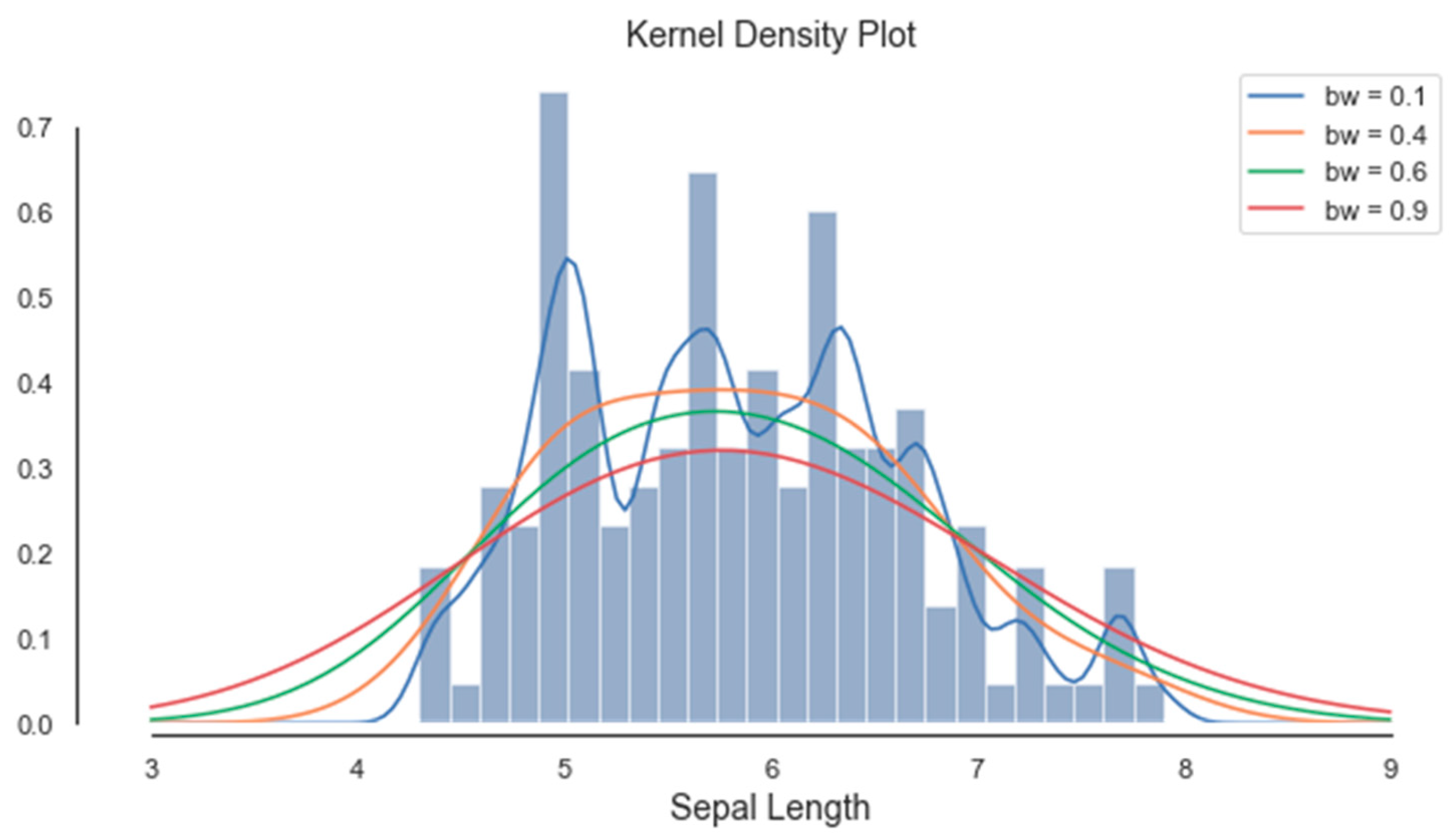
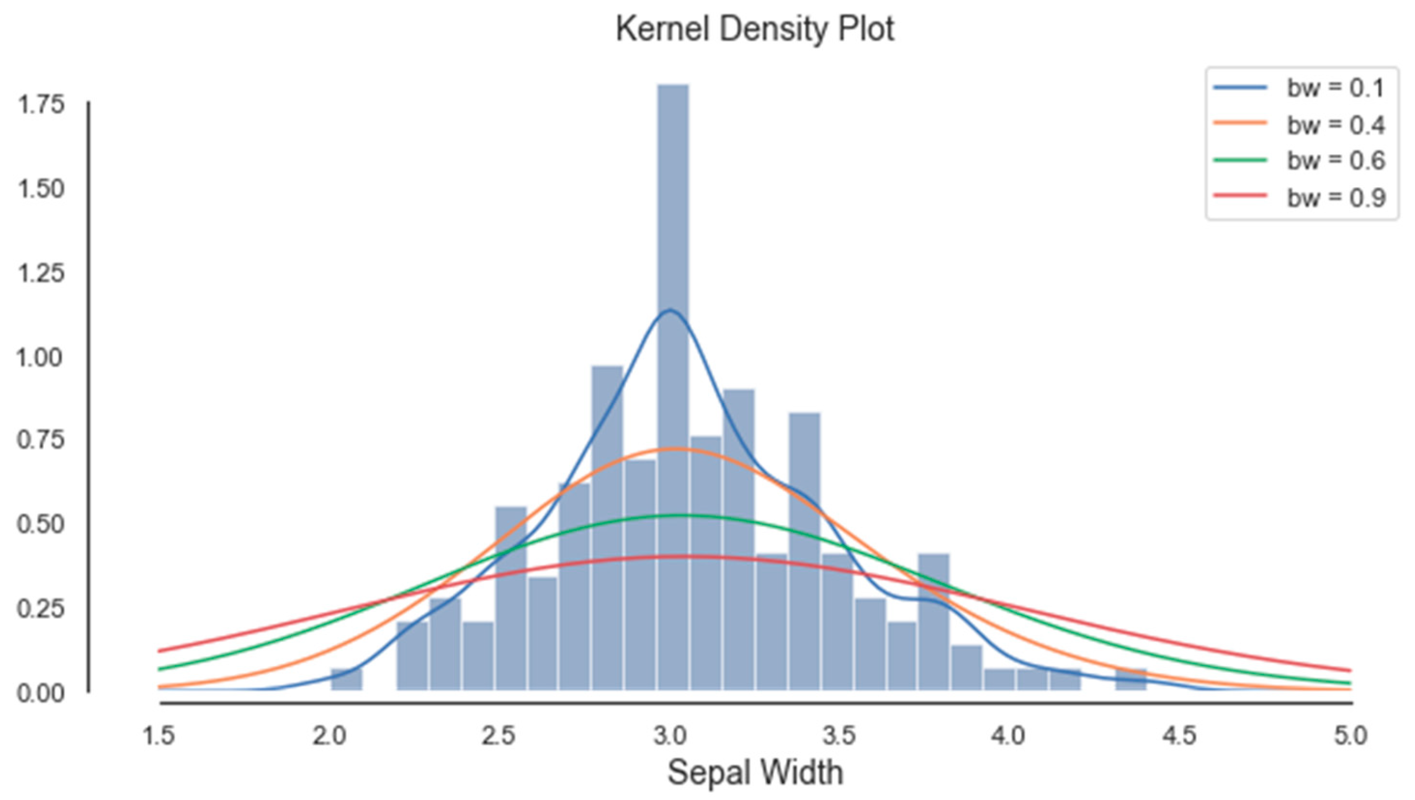
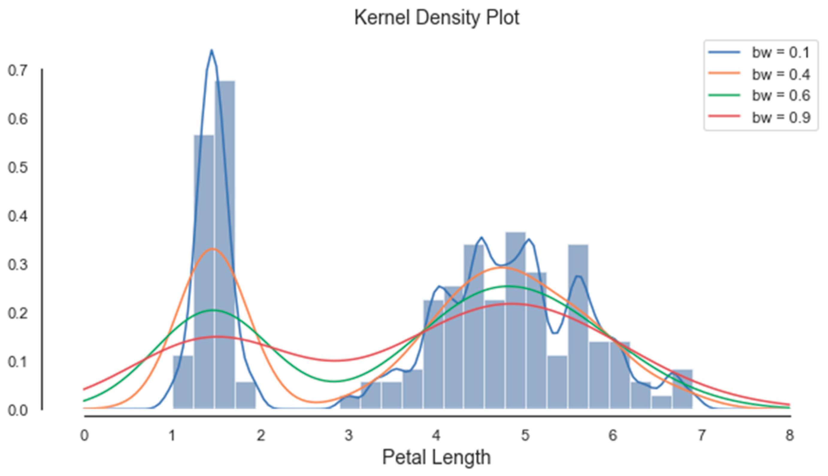
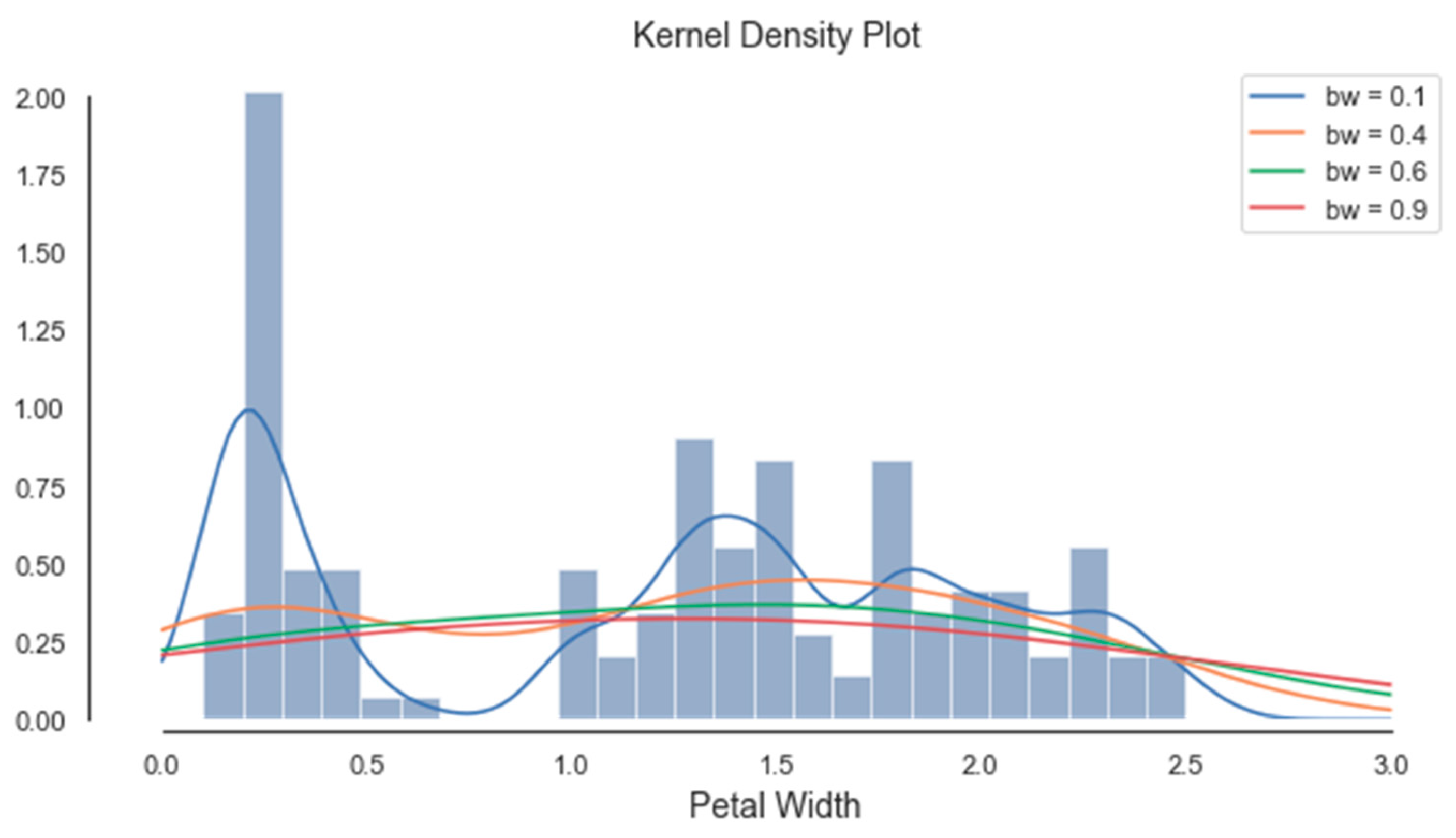
By applying the KDE technique for various bandwidth values, different segments were emphasized, and different thresholds were extracted (see Figure 8, Figure 9, Figure 10 and Figure 11). The optimal value for the bandwidth parameter is bw = 0.1, as it produces enough thresholds. After global segmentation, the Iris dataset had three classes produced by the two thresholds.

The attributes of sepal length, petal length and petal width had multimodal histograms. Their Gain Ratios are shown in

Table 1. Gain ratios of the attributes-Iris dataset.

Attribute	Gain Ratio
a1. sepal length	0.381
a2. sepal width	0.242
a3. petal length	0.734
a4. petal width	0.871

.

As expected, the Gain Ratio of the attribute that has an unimodal histogram (sepal width) was the lowest. The further procedure of the PPC method was based on the histogram segmentation of the attribute (a4) petal width, whose thresholds were 0.8 and 1.7.

Therefore, they produced three segments within the dataset. The arrangement of flowers is as follows:

• first segment: 50 setose flowers;
• second segment: 49 versicolor flowers and 5 virginica flowers;
• third segment: 1 versicolor flower and 45 virginica flowers.

The piecewise correlations were achieved on the three segments. The precise piecewise correlations on the segments are presented in

Table 2. Correlations on the first segment, produced by PPC method.

	a1	a2	a3	a4
a1	1
a2	0.74678	1
a3	0.263874	0.176695	1
a4	0.279092	0.279973	0.306308	1

,

Table 3. Correlations on the second segment, produced by PPC method.

	a1	a2	a3	a4
a1	1
a2	0.525412	1
a3	0.708887	0.39976	1
a4	0.498757	0.532008	0.750193	1

and

Table 4. Correlations on the third segment, produced by PPC method.

	a1	a2	a3	a4
a1	1
a2	0.350889	1
a3	0.865129	0.30595	1
a4	0.226632	0.418871	0.308638	1

.

4.2. Application on the Dryad Database

In an early stage of this research the segmentation was considered without the Gain Ratio. The achieved results are presented in [2]. The attributes of the interest [5] are as follows:

• Location-three types of terrain: Road, Grassy, Hills;
• Tag (ft)-the height of UAV in ft;
• Node position-Horizontal (Laid flat, parallel to the ground) or Vertical (Placed on edge on the ground);
• Velocity;
• Elevation;
• The real distance between the drone and sensor node (m); and
• Received Signal Strength Indicator (RSSI)

The RSSI was chosen for the decision attribute, and the others were influencing attributes.

The initial correlations among all attributes for horizontally placed nodes were very low, e.g., −0.091, 0.244, 0.082, 0.167, and 0.008 for location, tag or UAV high (ft), velocity, elevation, and real distance, respectively. The similar results are for vertically placed nodes: 0.005, 0.349, 0.108, 0.218, and 0.037.

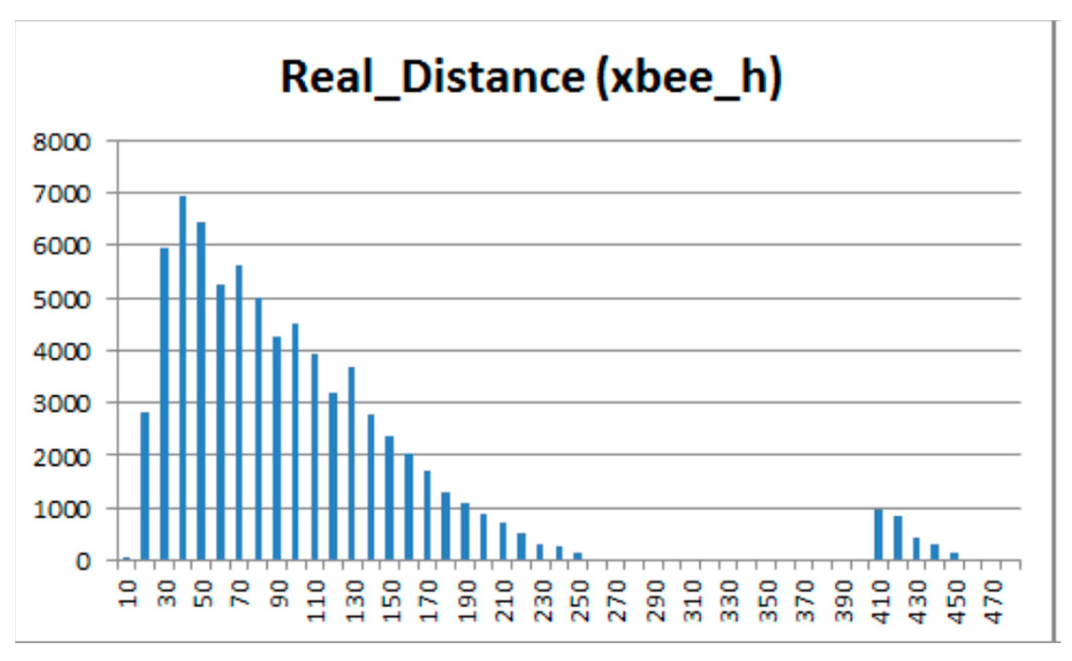
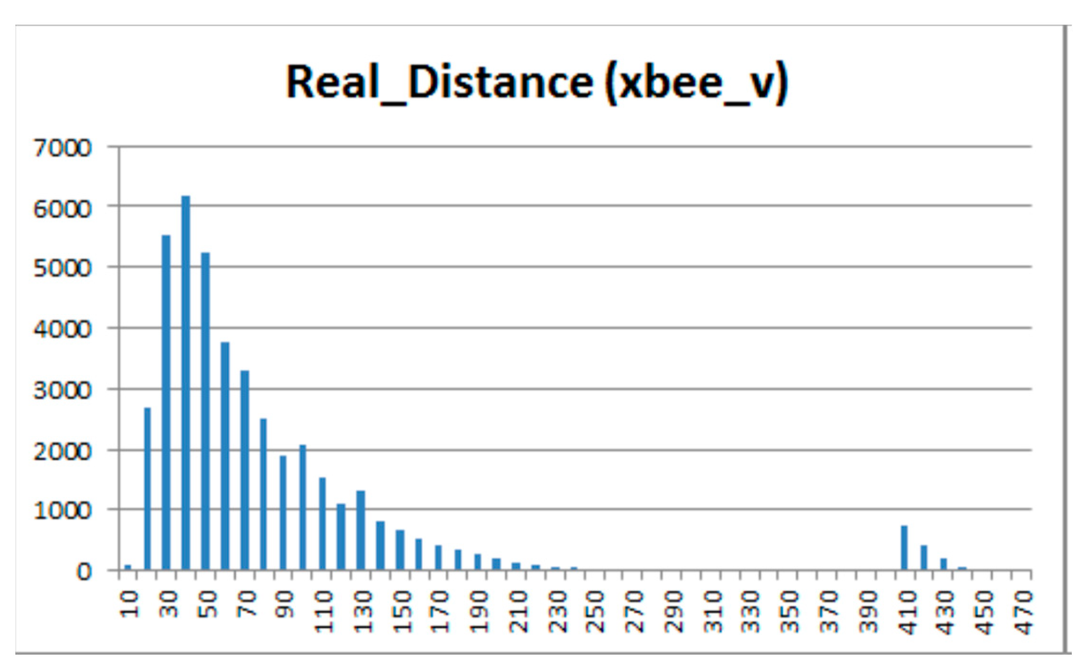
After histogram segmentation, the unimodal parts of the histogram concerning these attributes are obtained, and the bimodal distribution was detected. The correlations were calculated within each segment, separately (up to 400 m and between 400 and 500 m) for both horizontal (Figure 12) and vertical (Figure 13) node placements.

It was confirmed that correlations increased after the segmentation. Significantly higher correlations of the attribute RSSI with the attributes Tag, Elevation and Real Distance were observed.

4.3. Application on the Pima Indians Diabetes Database

The dataset was based on certain diagnostic measurements included in the dataset, while the class attribute-Outcome is information whether or not a patient has diabetes [6].

Attribute information:

• a1. Pregnancies (the number of pregnancies the patient has had)
• a2. Glucose
• a3. BloodPressure
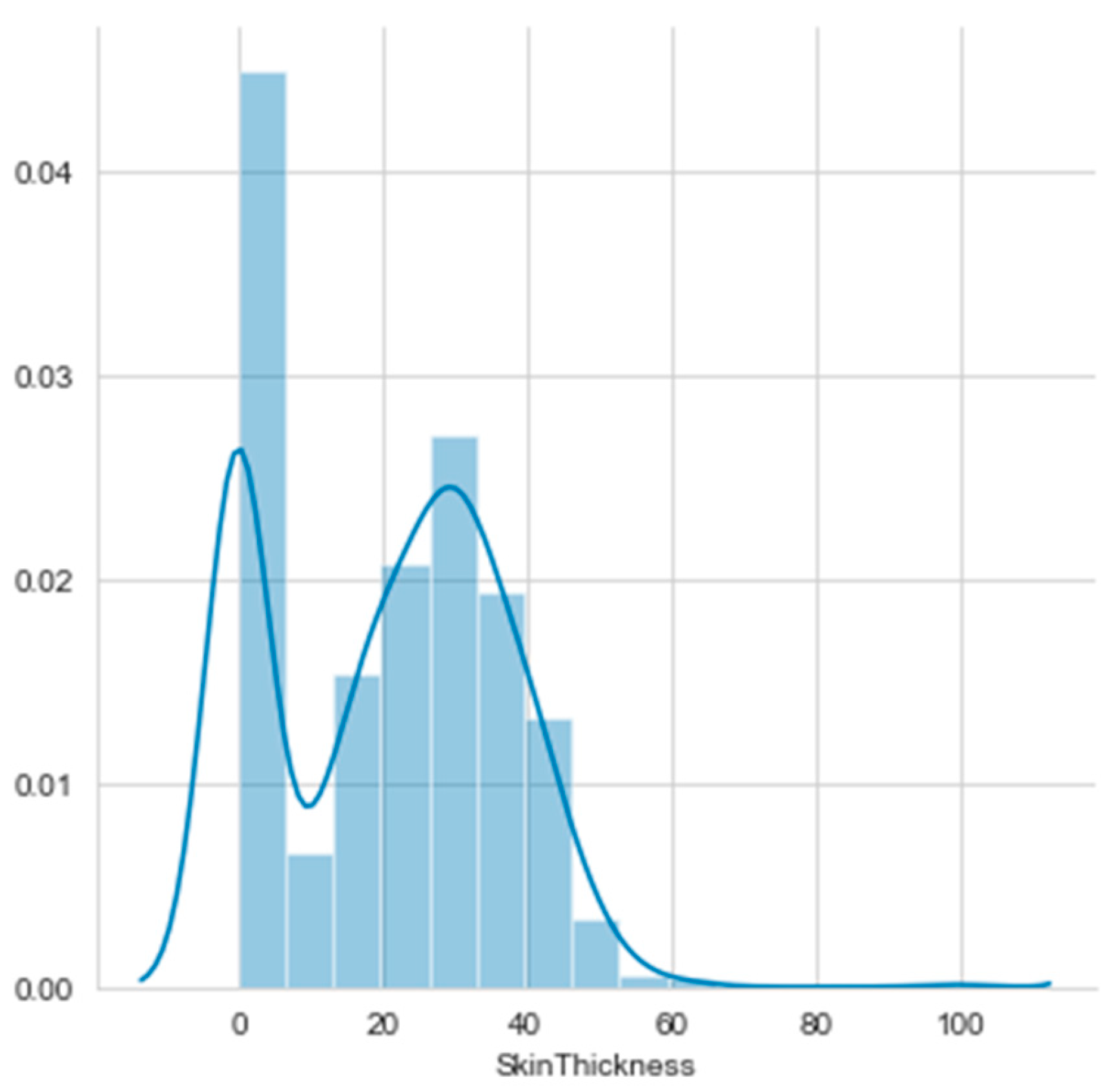
• a4. SkinThickness
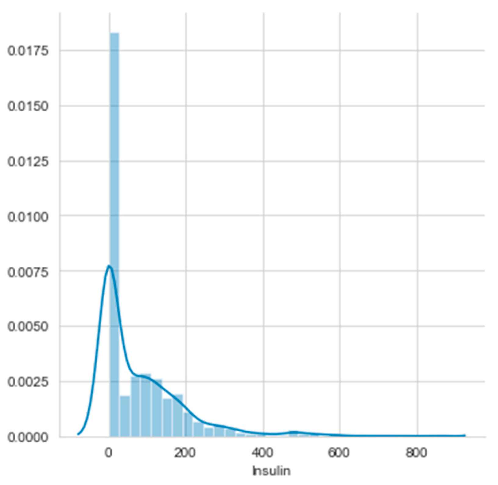
• a5. Insulin (insulin level)
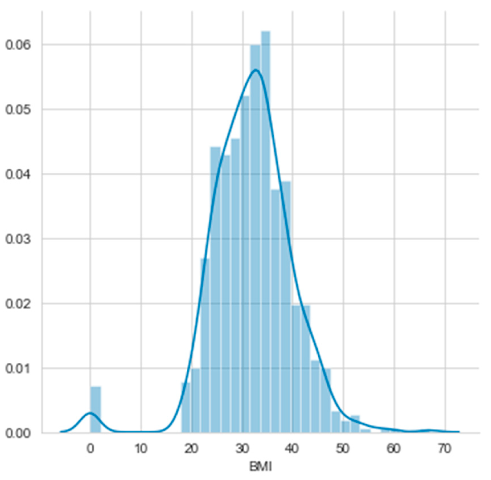
• a6. BMI
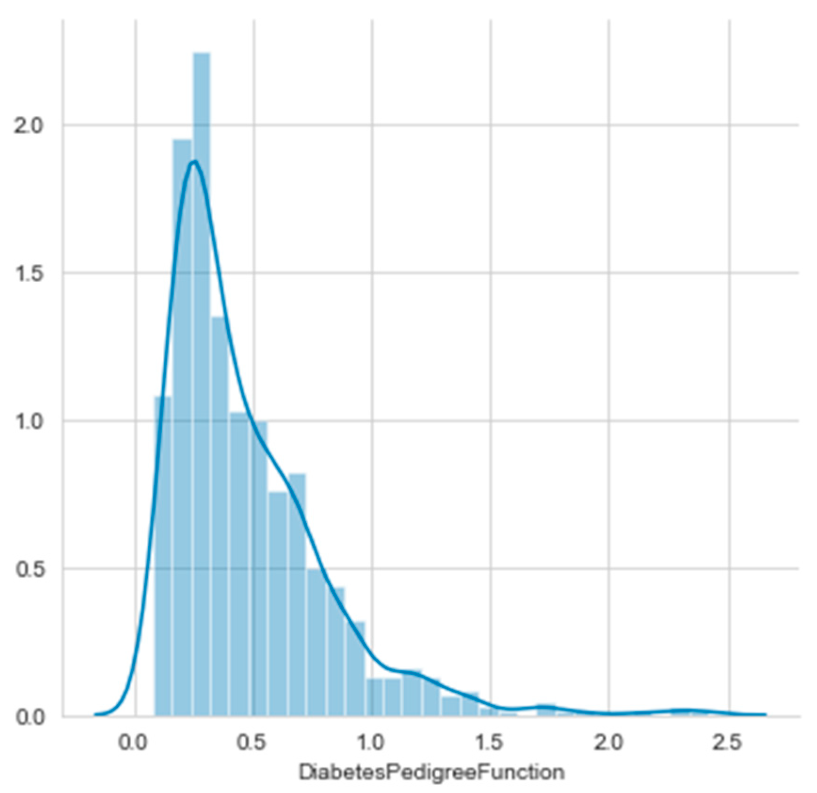
• a7. DiabetesPedigreeFunction
• a8. Age
• class, Outcome: 0-non-diabetes, 1-diabetes

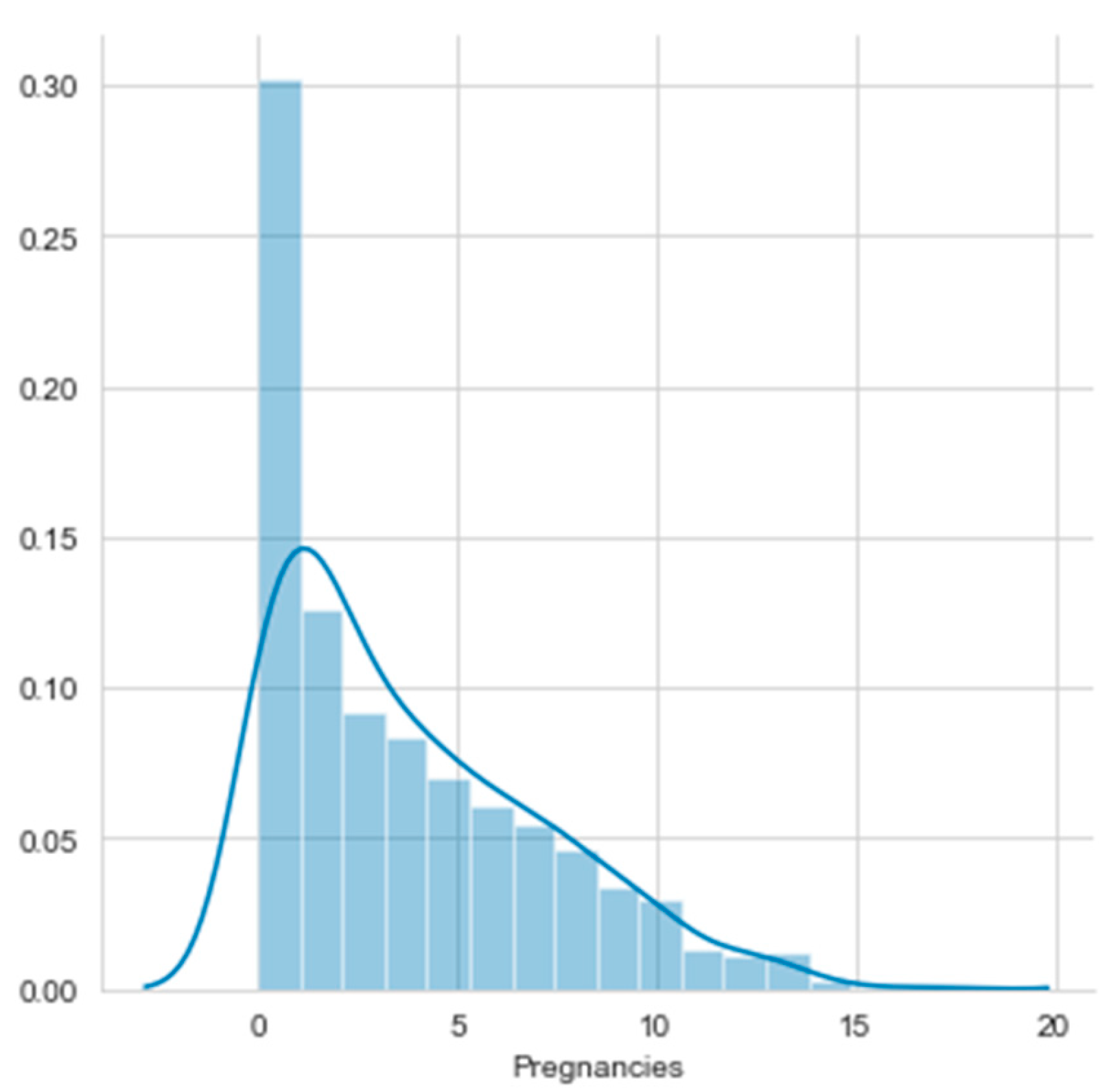
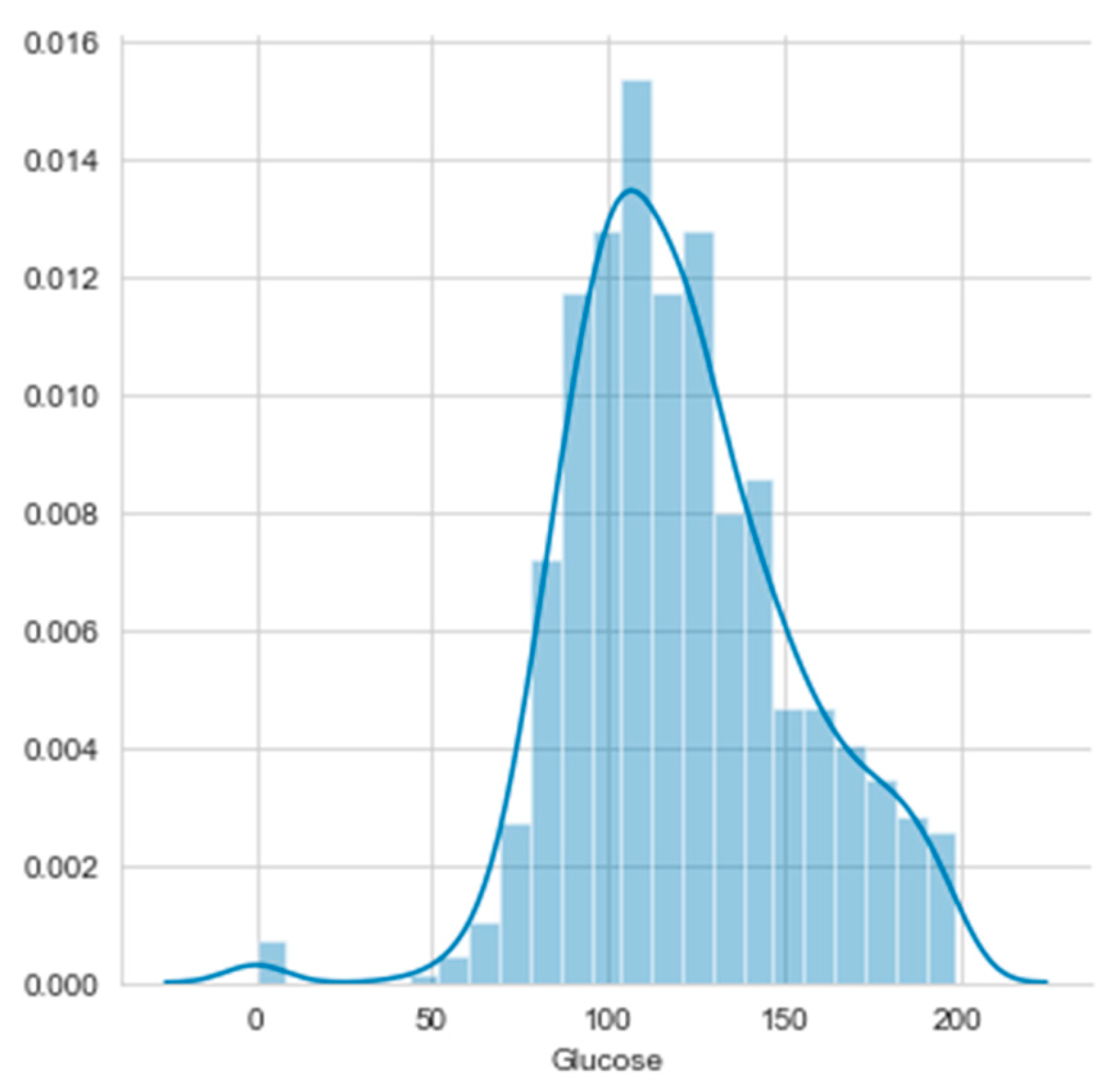
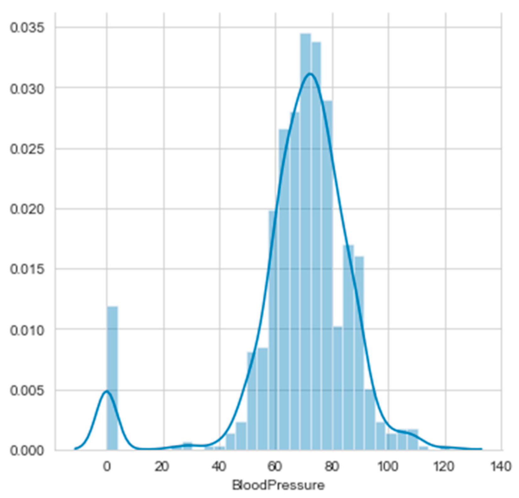
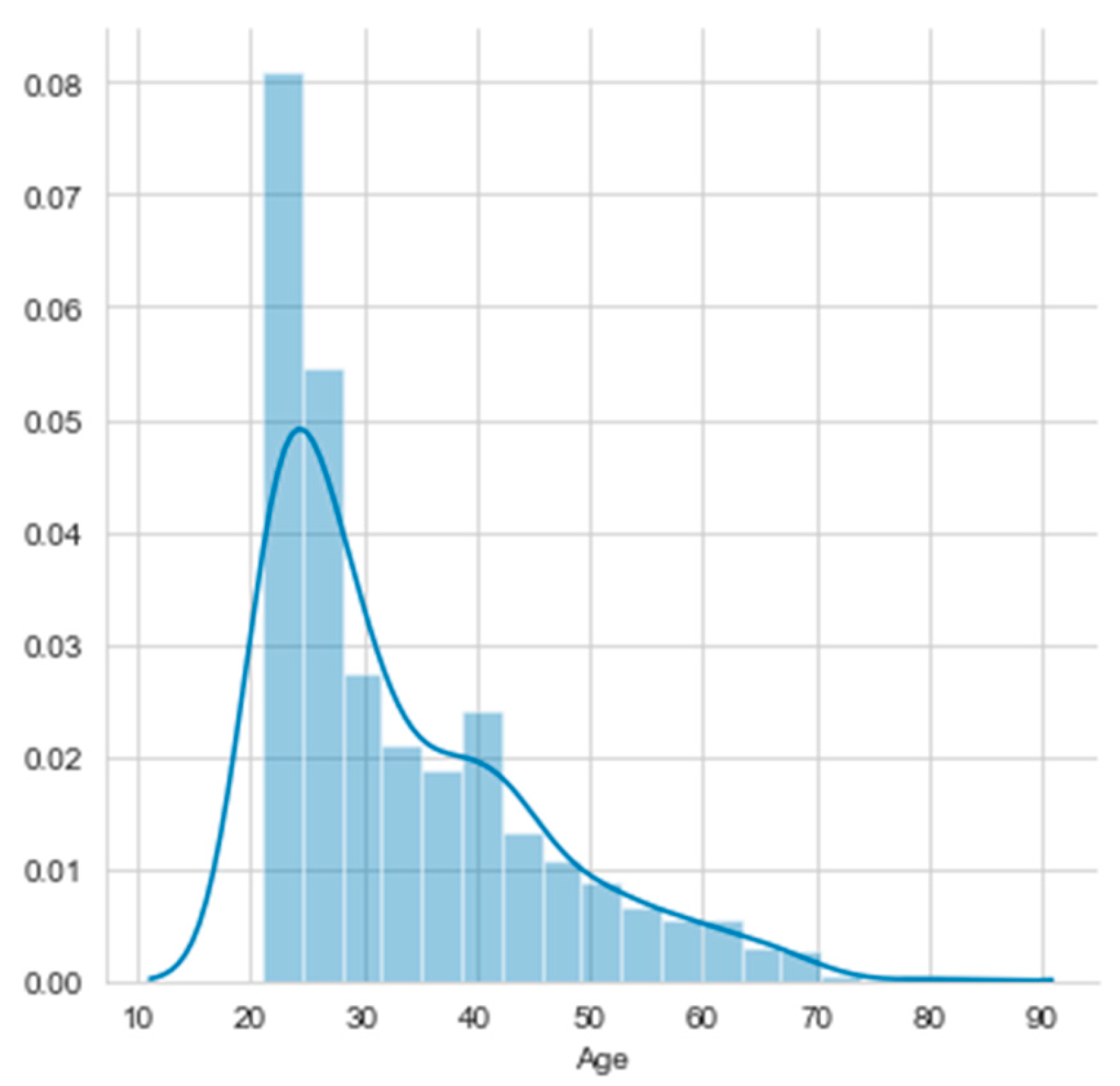
Histograms of the first eight attributes are generated and shown with associated KDE functions in Figure 14, Figure 15, Figure 16, Figure 17, Figure 18, Figure 19, Figure 20 and Figure 21.

The consideration of the attributes’ Gain Ratios produce very small values, as shown in

Table 5. Gain ratios of the attributes-Pima Indians Diabetes Database.

Attribute	Gain Ratio
a1. Pregnancies	0.0515
a2. Glucose	0.0986
a3. Blood Pressure	0.0144
a4. Skin Thickness	0.0224
a5. Insulin	0.0394
a6. BMI	0.0863
a7. Diabetes Pedigree Function	0.0226
a8. Age	0.0726

. The Glucose’s Gain Ratio is the highest, but its histogram has no distinguished unimodal parts. It is a case of more difficult histogram segmentation, but it was produced with the threshold 125.

Therefore, they produced two segments within the dataset. The deployment of patients is as follows:

• first segment: 379 non-diabetes patients and 92 diabetes patients;
• second segment: 121 non-diabetes patients and 176 diabetes patients.

The piecewise correlations were achieved on the two segments. The results are presented in

Table 6. Diabetes-Correlations on the first segment, produced by PPC method.

	a1	a2	a3	a4	a5	a6	a7	a8
a1	1
a2	0.055	1
a3	0.092	0.055	1
a4	−0.095	0.041	0.218	1
a5	−0.108	0.206	0.080	0.441	1
a6	0.014	0.051	0.377	0.440	0.225	1
a7	−0.017	0.023	0.043	0.135	0.189	0.066	1
a8	0.580	0.095	0.226	−0.107	−0.081	0.102	0.102	1

and

Table 7. Diabetes-Correlations on the second segment, produced by PPC method.

	a1	a2	a3	a4	a5	a6	a7	a8
a1	1
a2	0.048	1
a3	0.168	0.053	1
a4	−0.080	0.114	0.182	1
a5	−0.128	0.162	0.029	0.473	1
a6	−0.046	0.114	0.059	0.326	0.099	1
a7	−0.083	0.118	0.001	0.227	0.146	0.192	1
a8	0.486	0.124	0.195	−0.157	−0.156	−0.191	−0.091	1

.

4.4. Application on the Glass Dataset

In the next iteration, the PPC method has been applied on the Glass dataset [7]. According to the USA Forensic Science Service this dataset contains 6 types of glass defined in terms of their oxide content. The attribute information is as follows:

• Id number: 1 to 214 (removed from CSV file)
• a1. RI: refractive index
• a2. Na: Sodium (unit measurement: weight percent in corresponding oxide, as are attributes 4–10)
• a3. Mg: Magnesium
• a4. Al: Aluminum
• a5. Si: Silicon
• a6. K: Potassium
• a7. Ca: Calcium
• a8. Ba: Barium
• a9. Fe: Iron
• Type of glass: (class attribute):

  --

  1 building_windows_float_processed

  --

  2 building_windows_non_float_processed

  --

  3 vehicle_windows_float_processed

  --

  4 vehicle_windows_non_float_processed (none in this database)

  --

  5 containers

  --

  6 tableware

  --

  7 headlamps

All attributes have multimodal histograms but not according to the number of class attribute values. Their Gain Ratios are shown in

Table 8. Gain Ratios of the attributes-Glass dataset.

Attribute	Gain Ratio
a1. RI	0.221
a2. Na	0.475
a3. Mg	0.653
a4. Al	0.386
a5. Si	0.0
a6. K	0.356
a7. Ca	0.322
a8. Ba	0.72
a9. Fe	0.121

.

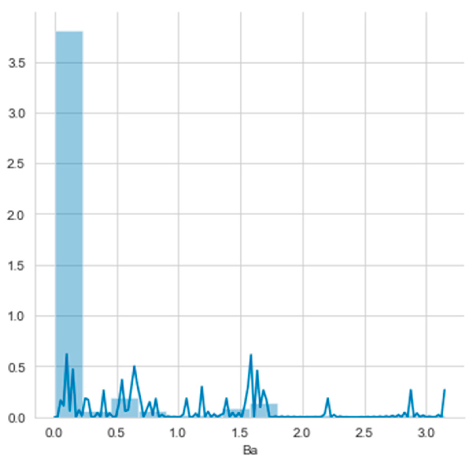
Attribute a8. Ba has the highest Gain Ratio, but the histogram of Ba (Figure 22) did not have five thresholds, according to the number of class attribute values.

5. Discussion

5.1. Discussion-Iris Dataset

For the purpose of comparison of the PPC method results, the initial correlation (see

Table 9. Initial correlation-Iris dataset.

	a1	a2	a3	a4
a1	1
a2	−0.10937	1
a3	0.871754	−0.42052	1
a4	0.817954	−0.35654	0.962757	1

) and correlations by the flower types (setosa, versicolor and virginica) are computed (see

Table 10. Correlation within the setosa flower type.

	a1	a2	a3	a4
a1	1
a2	0.74678	1
a3	0.263874	0.176695	1
a4	0.279092	0.279973	0.306308	1

,

Table 11. Correlation within the versicolor flower type.

	a1	a2	a3	a4
a1	1
a2	0.525911	1
a3	0.754049	0.560522	1
a4	0.546461	0.663999	0.786668	1

and

Table 12. Correlation within the virginica flower type.

	a1	a2	a3	a4
a1	1
a2	0.457228	1
a3	0.864225	0.401045	1
a4	0.281108	0.537728	0.322108	1

).

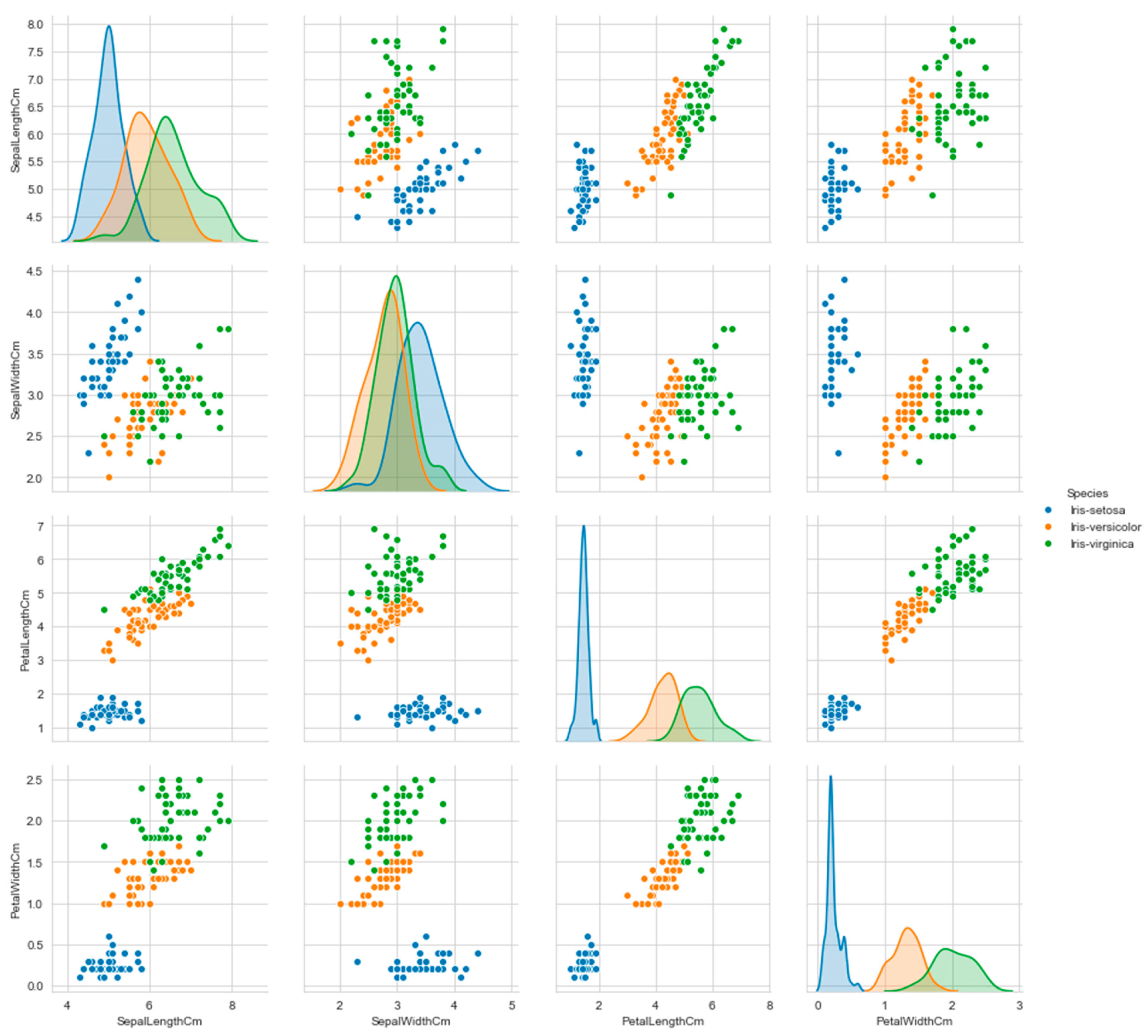
The overall correlations of the attributes of all flower types are supported by Figure 23, which contains scatter plots with the three colors that indicate the three classes in the data. The KDE functions of the attributes are included on the diagonal. The consideration of only one color in the scatter plots is associated with the correlation by flower type (blue-setosa, orange-versicolor, green-virginica).

The dots’ positions on the scatter plots a3-a1 (petal length and sepal length), a4-a1 (petal width and sepal length) and a4-a3 (petal width and petal length) indicate noticeable correlations, while on the other plots the dots are too scattered. On the other hand, if considering colors of the dots (by flower type), the high correlations of the following attributes are very noticeable: a1-a2 (sepal length and sepal width) in setose, a1-a3 (sepal length and petal length) and a3-a4 (petal length and petal width) in versicolor, and a1-a3 (sepal length and petal length) in virginica.

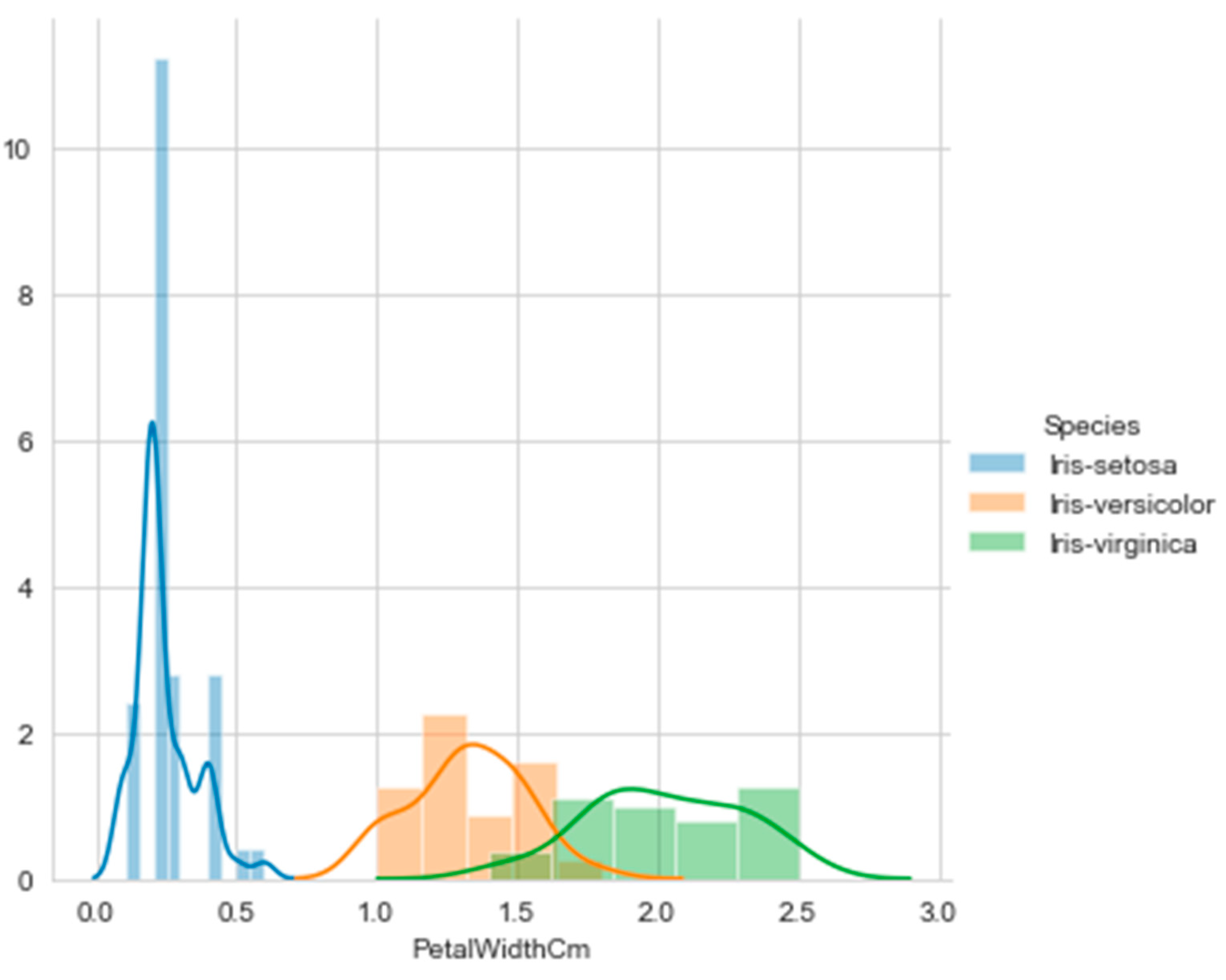
A very interesting matching has to be underlined. Namely, significant thresholds produced by the a4 histogram segmentation (0.8 and 1.7) do coincide with the intersection of the KDE functions associated to the histograms considered individually by the flower type. The intersections (blue-orange and orange-green) are visible in Figure 24. The produced segmentation of the entire dataset coincided with the natural classification that exists by flower type. This is another confirmation of the validity of histogram segmentation.

The largest match in correlation is obtained in the case when the segmentation of the dataset is carried out based on the histogram segmentation of the attribute with the highest Gain Ratio.

To verify the previous statement, the segmentation of the dataset was carried out according to the histogram segmentation of the first and third attributes. The results are presented in Section 5.1.1 and Section 5.1.2.

5.1.1. Correlation Based on a1. Sepal Length Histogram Segmentation

The KDE of the attribute sepal length has significant thresholds at 5.3 and 6.1 (see Figure 9). Therefore, the piecewise correlation will be achieved on the three segments, which are presented in

Table 13. Correlation within first segment after a1. sepal length histogram segmentation.

	a1	a2	a3	a4
a1	1
a2	0.301879	1
a3	0.264377	−0.61853	1
a4	0.237265	−0.58633	0.95083	1

,

Table 14. Correlation within second segment after a1. sepal length histogram segmentation.

	a1	a2	a3	a4
a1	1
a2	−0.26648	1
a3	0.582701	−0.75851	1
a4	0.495901	−0.62714	0.932693	1

and

Table 15. Correlation within third segment after a1. sepal length histogram segmentation.

	a1	a2	a3	a4
a1	1
a2	0.319041	1
a3	0.713599	0.314832	1
a4	0.267713	0.423937	0.694508	1

.

The arrangement of the flowers is as follows:

• first segment: 40 setose flowers, 5 versicolor flowers, and 1 virginica flower
• second segment: 10 setose flowers, 29 versicolor flowers, and 10 virginica flowers
• third segment: 16 versicolor flower and 39 virginica flowers.

Table 13, Table 14 and Table 15 show a noticeable greater deviation from the correlations given in Table 10, Table 11 and Table 12 with respect to the result of the PPC method.

5.1.2. Correlation Based on a3. Petal Length Histogram Segmentation

The KDE of the attribute sepal length has significant thresholds at 2.1 and 4.8 (see Figure 10). Therefore, the piecewise correlation will be achieved on the three segments, which are presented in

Table 16. Correlation within first segment after a3. petal length histogram segmentation.

	a1	a2	a3	a4
a1	1
a2	0.74678	1
a3	0.263874	0.176695	1
a4	0.279092	0.279973	0.306308	1

,

Table 17. Correlation within second segment after a3. petal length histogram segmentation.

	a1	a2	a3	a4
a1	1
a2	0.533064	1
a3	0.681651	0.598278	1
a4	0.378072	0.606714	0.759463	1

and

Table 18. Correlation within third segment after a3. petal length histogram segmentation.

	a1	a2	a3	a4
a1	1
a2	0.437	1
a3	0.81299	0.378817	1
a4	0.220331	0.517164	0.356475	1

.

The arrangement of flowers is as follows:

• first segment: 50 setose flowers,
• second segment: 46 versicolor flowers and 3 virginica flowers,
• third segment: 4 versicolor flower and 47 virginica flowers.

Table 16, Table 17 and Table 18 show less deviation from the correlations given in Table 13, Table 14 and Table 15 with respect to the result of the PPC method.

It is worth noting that the Gain Ratio and distribution plot by class are evidently related. Namely, the higher Gain Ratio corresponds to the histogram with less overlapping of the unimodal parts (see

Table 19. Iris-Gain Ratio and distplot by class, of all attributes.

Gain Ratio	Distplot by Class
0.871
0.734
0.381
0.242

).

5.2. Discussion-Dryad Database

There is a high probability that measured data has histogram with unimodal parts supported by Gaussian normal distribution [28,29]. Therefore, it is justified to check the correlation on the histogram segments, even without considering the Gain Ratio.

In relation to the overall correlation of the dataset, which was initially not significant, after segmentation, the obtained correlations on the separated segments are very useful for further use.

5.3. Discussion-Pima Indian Diabetes Database

For the purpose of comparison of the PPC method results, the initial correlation (see

Table 20. Initial correlation-Pima Indian Diabetes dataset.

	a1	a2	a3	a4	a5	a6	a7	a8
a1	1
a2	0.129	1
a3	0.141	0.153	1
a4	−0.082	0.057	0.207	1
a5	−0.074	0.331	0.089	0.437	1
a6	0.018	0.221	0.282	0.393	0.198	1
a7	−0.034	0.137	0.041	0.184	0.185	0.141	1
a8	0.544	0.264	0.240	−0.114	−0.042	0.036	0.034	1

) and correlations by class (non-diabetes and diabetes) are computed (see

Table 21. Correlation within the class 0 (non-diabetes).

	a1	a2	a3	a4	a5	a6	a7	a8
a1	1
a2	0.099	1
a3	0.133	0.193	1
a4	−0.118	0.016	0.187	1
a5	−0.132	0.353	0.075	0.413	1
a6	0.016	0.132	0.363	0.439	0.254	1
a7	−0.080	0.096	0.027	0.095	0.227	0.071	1
a8	0.573	0.228	0.215	−0.164	−0.149	0.036	0.042	1

and

Table 22. Correlation within the class 1 (diabetes).

	a1	a2	a3	a4	a5	a6	a7	a8
a1	1
a2	−0.055	1
a3	0.127	0.069	1
a4	−0.079	0.038	0.225	1
a5	−0.079	0.261	0.0896	0.457	1
a6	−0.159	0.050	0.134	0.312	0.055	1
a7	−0.069	0.026	0.035	0.274	0.102	0.137	1
a8	0.445	0.099	0.263	−0.092	0.024	−0.188	−0.088	1

).

The largest matches in correlation are obtained when the segmentation of the dataset is carried out based on the histogram segmentation of the attribute with the highest Gain Ratio.

Table 21 and Table 22 show less deviation from the correlations given in the result of the PPC method (Table 6 and Table 7).

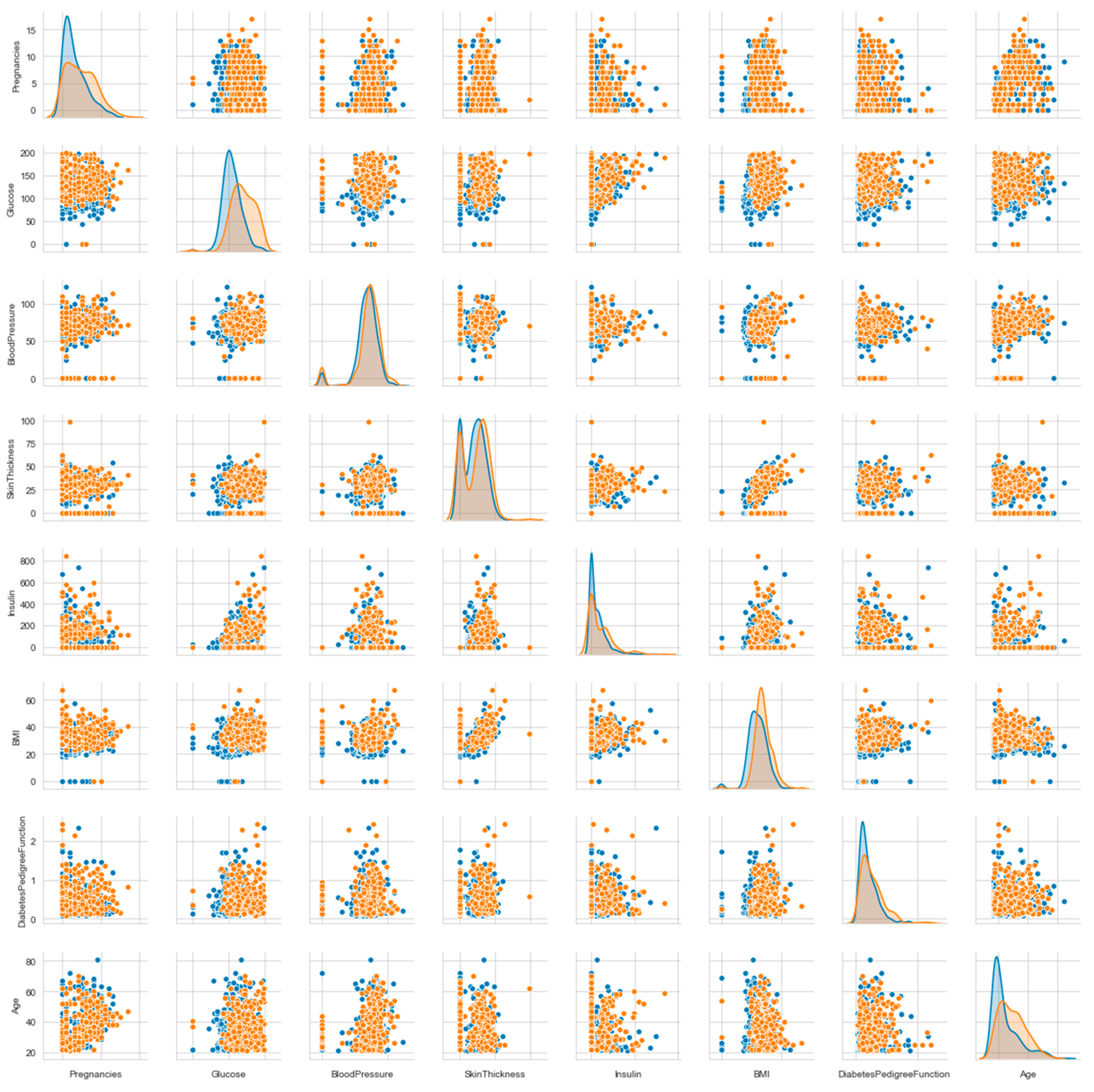
The overall correlations of the attributes of all diabetes types are supported by Figure 25, which contains scatter plots with the two colors that indicate the two classes in the data. The KDE functions of the attributes are included on the diagonal. Consideration of only one color in the scatter plots is associated with the correlation by patient type (non-diabetes and diabetes).

Again, the Gain Ratio and distribution plot by class are related. The higher Gain Ratio corresponds to the histogram with less overlapping of the unimodal parts (see

Table 23. Gain Ratio and corresponding distplot by class.

Gain Ratio	Distplot by Class	Gain Ratio	Distplot by Class
0.0986		0.0394
0.0863		0.0226
0.0726		0.0224
0.0515		0.0144

).

Unlike the Iris dataset, Pima Indian Diabetes does not have an attribute with a sufficiently high Gain Ratio whose histogram has separated unimodal parts.

5.4. Discussion-Glass Dataset

Glass dataset has the attributes with multimodal histogram and high Gain Ratio, but the PPC method is not applicable: the histograms of attributes with the highest Gain Ratios have no segmentation according to the number of class attribute values. The Glass dataset has the class attribute with six types of glass. For seven segmented parts, five thresholds are required.

For datasets with multiple values of the class attribute, there is often a multiple overlap of KDF functions corresponding to a particular class. In that case segmentation of the histogram is not possible.

6. Conclusions

The method for the determination of the precise piecewise correlation after histogram segmentation has been created. All the used classic tools and methods were briefly presented with details of their infiltration in the PPC method. The method has been exposed by the single steps and diagram, and tested by application on the Iris, Dryad, Pima Indian Diabetes, and Glass datasets. The results were compared with classical correlations produced on the entire dataset and its existed classes, and they confirm that the classes could be neglected. In other words, when Gain Ratio has high value, classes within the dataset are not crucial for the piecewise correlation. All previous considerations confirm that the PPC method is suitable for segmentation and piecewise correlation of a dataset in case any classification is missing. Detected correlations revealed the strength and nature of the symmetric association between two attributes on each separated segment.

This research reveals connection between the Gain Ratio and similarity of the correlation on segments (after histogram segmentation) with correlation by classes. Further, it is challenging to detect a threshold of the Gain Ratio that will provide a correlation similar enough to the correlation by classes.

The possibilities of applying the PPC method are great because histograms are an integral part of basic data analysis. The PPC method is beneficial for considering the possibility of effective data division into clusters.

Further work will concern testing the PPC method on more datasets.

References

- Lindblad, J. Histogram Thresholding using Kernel Density Estimates. In Proceedings of the Swedish Society for Automated Image Analysis (SSAB) Symposium on Image Analysis, Halmstad, Sweden; 2000; pp. 41–44. [Google Scholar]
- Dobrilovic, D.; Ognjenovic, V.; Berkovic, I.; Radosav, D. Analyses of WSN/UAV network configuration influences on 2.4 GHz IEEE 802.15.4 signal strength. In Proceedings of the 2021 International Telecommunications Conference (ITC-Egypt), Alexandria, Egypt, 13–15 July 2021; pp. 1–5. [Google Scholar] [CrossRef]
- Ognjenovic, V. Approximative Discretization of Table-Organized Data. Ph.D. Thesis, Technical Faculty “Mihajlo Pupin”, University of Novi Sad, Zrenjanin, Serbia, 2016. Available online: https://nardus.mpn.gov.rs/bitstream/handle/123456789/8685/Disertacija13338.pdf?sequence=6&isAllowed=y (accessed on 1 February 2024). (In Serbian).
- Iris.csv—Kaggle. 2023. Available online: https://www.kaggle.com/datasets/saurabh00007/iriscsv (accessed on 1 February 2024).
- Nekrasov, M.; Allen, R.; Belding, E. Aerial Measurements from Outdoor 2.4GHz 802.15.4 Network. Dryad, Dataset. 2019. Available online: https://datadryad.org/stash/dataset/doi%253A10.25349%252FD9KS3 (accessed on 2 April 2021).
- Pima Indians Diabetes Database.csv—Kaggle. 2024. Available online: https://www.kaggle.com/datasets/uciml/pima-indians-diabetes-database (accessed on 2 April 2024).
- Glass.csv—Kaggle. 2024. Available online: https://www.kaggle.com/datasets/uciml/glass (accessed on 5 March 2024).
- Pearson, K. Notes on regression and inheritance in the case of two parents. Proc. R. Soc. Lond. 1895, 58, 240–242. [Google Scholar]
- Asuero, A.G.; Sayago, A.; Gonzalez, A.G. The correlation coefficient. An Overview. Crit. Rev. Anal. Chem. 2006, 36, 41–59. [Google Scholar] [CrossRef]
- Atmanspacher, H.; Martin, M. Correlations and How to Interpret Them. Information 2019, 10, 272. [Google Scholar] [CrossRef]
- Jiang, Y.; Chen, Y.; Tian, R.; Wang, L.; Lv, S.; Lin, J.; Xing, X. Application of the Segmented Correlation Technology in Seismic Communication with Morse Code. Appl. Sci. 2021, 11, 1947. [Google Scholar] [CrossRef]
- Ognjenovic, V.; Brtka, V.; Stojanov, J.; Brtka, E.; Berkovic, I. The Cuts Selection Method Based on Histogram Segmentation and Impact on Discretization Algorithms. Entropy 2022, 24, 675. [Google Scholar] [CrossRef] [PubMed]
- Chang, J.H.; Fan, K.C.; Chang, Y.L. Multi-modal gray-level histogram modeling and decomposition. Image Vis. Comput. 2002, 20, 203–216. [Google Scholar] [CrossRef]
- Sahoo, P.K.; Soltani, S. A survey of thresholding techniques. Comput. Vis. Graph. Image Process. 1988, 41, 233–260. [Google Scholar] [CrossRef]
- Kwon, S.H. Threshold selection based on cluster analysis. Pattern Recognit. Lett. 2004, 25, 1045–1050. [Google Scholar] [CrossRef]
- Gopalakrishnan, S.; Kandaswamy, A. Automatic Delineation of Lung Parenchyma Based on Multilevel Thresholding and Gaussian Mixture Modelling. Comput. Model. Eng. Sci. 2018, 114, 141–152. [Google Scholar]
- Arifin, Z.; Asano, A. Image segmentation by histogram thresholding using hierarchical cluster analysis. Pattern Recognit. Lett. 2006, 27, 1515–1521. [Google Scholar] [CrossRef]
- Mohapatra, S.; Patra, D.; Kumar, K. Blood microscopic image segmentation using rough sets. In Proceedings of the 2011 International Conference on Image Information Processing (ICIIP), Shimla, India, 3–5 November 2011. [Google Scholar]
- Xie, C.H.; Liu, Y.-J.; Chang, J.-Y. Medical image segmentation using rough set and local polynomial regression. Multimed. Tools Appl. 2015, 74, 1885–1914. [Google Scholar] [CrossRef]
- Hafemann, L.G.; Sabourin, R.; Oliveira, L.S. Learning features for offline handwritten signature verification using deep convolutional neural networks. Pattern Recognit. 2017, 70, 163–176. [Google Scholar] [CrossRef]
- Rosin, P.L. Unimodal thresholding. Pattern Recognit. 2001, 34, 2083–2096. [Google Scholar] [CrossRef]
- Węglarczyk, S. Kernel density estimation and its application. In ITM Web of Conferences; EDP Sciences: Ulys, France, 2018; Volume 23, p. 00037. [Google Scholar] [CrossRef]
- The Importance of Kernel Density Estimation Bandwidth, February 2023. Available online: https://aakinshin.net/posts/kde-bw/ (accessed on 1 March 2024).
- Cover, T.M.; Thomas, J.A. Elements of Information Theory; John Wiley & Sons, Inc.: Hoboken, NJ, USA, 2006. [Google Scholar]
- Hastie, T.; Tibshirani, R.; Friedman, J. The Elements of Statistical Learning in Data Mining, Inference, and Prediction, 2nd ed.; Springer: Berlin/Heidelberg, Germany, 2009. [Google Scholar]
- Sam, T. Entropy: How Decision Trees Make Decisions. 2024. Available online: https://towardsdatascience.com/entropy-how-decision-trees-make-decisions-2946b9c18c8 (accessed on 1 February 2024).
- Singh, A. Decision Trees, Machine Learning 10-315. 2 November 2020. Available online: https://www.cs.cmu.edu/~aarti/Class/10315_Fall20/lecs/DecisionTrees.pdf (accessed on 1 February 2024).
- Williams, R. Normal Distribution. University of Notre Dame. 2024. Available online: https://www3.nd.edu/~rwilliam/stats1/x21.pdf (accessed on 2 April 2024).
- Gaedke, U.; Klauschies, T. Analyzing the Shape of Observed Trait Distributions Enables a Data-Based Moment Closure of Aggregate Models. Limnology and Oceanography: Methods. 2017. Available online: https://aslopubs.onlinelibrary.wiley.com/doi/10.1002/lom3.10218 (accessed on 2 April 2024). [CrossRef]
Figure 1.
(a) Original image of blood; (b) gray-level histogram of the image; (c) smoothed histogram with threshold values; (d) the blood cells; (e) blood-plasma; (f) the cell membrane (overtaken from [13]).
Figure 2.
Example of histogram and KDE.
Figure 3.
PPC method.
Figure 4.
Histogram and KDE of a1. sepal length.
Figure 5.
Histogram and KDE of a2. sepal width.
Figure 6.
Histogram and KDE of a3. petal length.
Figure 7.
Histogram and KDE of a4. petal width.
Figure 8.
KDE of a1. sepal length for various parameters bw.
Figure 9.
KDE of a2. sepal width for various parameters bw.
Figure 10.
KDE of a3. petal length for various parameters bw.
Figure 11.
KDE of a4. petal width for various parameters bw.
Figure 12.
Data histogram of real distance for horizontal nodes.
Figure 13.
Data histogram of real distance for vertical nodes.
Figure 14.
Histogram and KDE of a1. Pregnancies.
Figure 15.
Histogram and KDE of a2. Glucose.
Figure 16.
Histogram and KDE of a3. BloodPressure.
Figure 17.
Histogram and KDE of a4. SkinThickness.
Figure 18.
Histogram and KDE of a5. Insulin.
Figure 19.
Histogram and KDE of a6. BMI.
Figure 20.
Histogram and KDE of a7. DiabetesPedigreeFunction.
Figure 21.
Histogram and KDE of a8. Age.
Figure 22.
Histogram and KDE of Ba (Barium).
Figure 23.
Scatter plots of the attributes of all iris flower types.
Figure 24.
KDE functions of a4. petal width.
Figure 25.
Scatter plots of the attributes of non-diabetes and diabetes.