
Bayesian Inference of Recurrent Switching Linear Dynamical Systems with Higher-Order Dependence


Abstract
1. Introduction
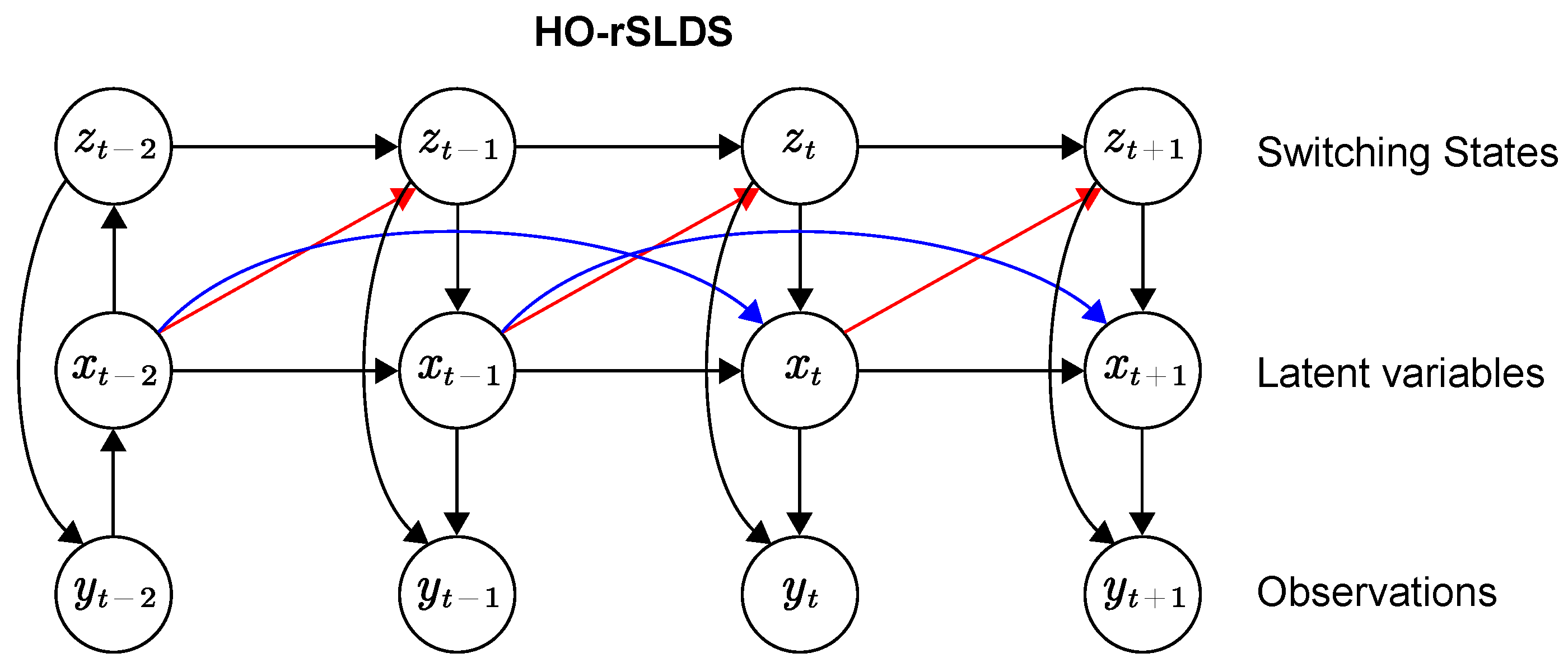
- HO-rSLDS assumes the linear dynamics of latent variables can be described by a higher-order VAR process, which makes it feasible to dig out and evaluate the long-term dependency relationships from dynamical phenomena;
- Stick-breaking logistic regression is applied to determine the switching state transition in HO-rSLDS. By this means, the transition probabilities are time-varying and can be adjusted according to the previous latent variable, which overcomes the limitation of restricted geometric state duration time by Markov assumption and recovers the symmetric dependency between the switching states and the latent variable;
- The Pólya-gamma augmentation strategy permits efficient Bayesian inference algorithms. In addition, we propose message-passing algorithms, including a forward Kalman filter and backward Kalman smoother for HO-rSLDS, which facilitates the parameter update in variational inference.
2. Methods
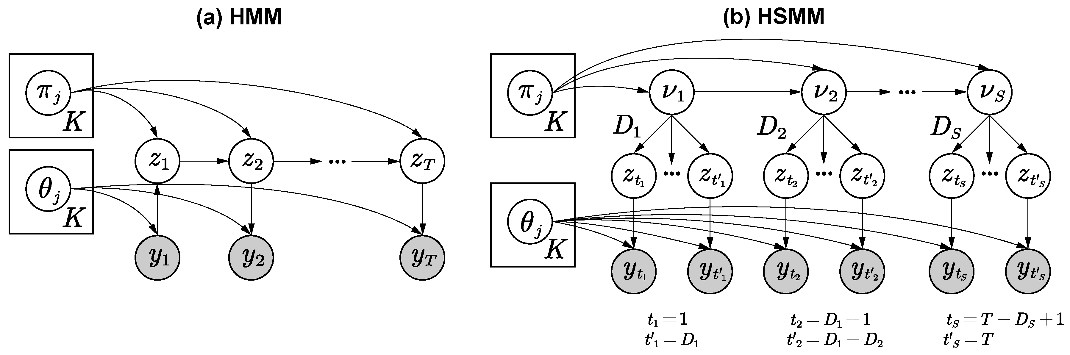
2.1. HMM and HSMM
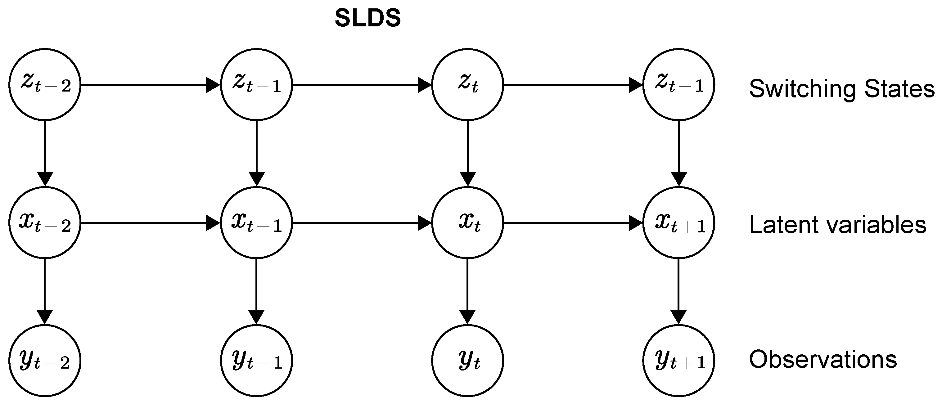
2.2. SLDS
2.3. Recurrent Switching Linear Dynamic System with Higher-Order Dependence
2.3.1. HO-SLDS
2.3.2. Stick-Breaking Logistic Regression and Pólya-Gamma Augmentation for HO-SLDS
3. Variational Inference of HO-rSLDS
3.1. Update for
| Algorithm 1: Obtaining |
 |
3.2. Update for
3.3. Update for
| Algorithm 2: Obtaining |
 |
3.4. Update for
- Update . Simplifying Equation (38) and extracting the terms related to , we havewhich results inwhere andare prior parameters of .
- Update . The posterior can be obtained by the expectations of , given by
- Update . Simplifying Equation (38) and extracting the terms related to , we havewhich results inwhere ,The variational posterior parameters can be optimized aswhere are prior parameters of .
- Update . Simplifying Equation (38) and extracting the terms related to , we havewhich results inwhere ,The variational posterior parameters can be optimized aswhere are prior parameters of .
- Update . Simplifying Equation (38) and extracting the terms related to , we havewhich results inwhere , which can be optimized asand are prior parameters of . To derive Equation (107), just note that and use the matrix trace.
- Update . Simplifying Equation (38) and extracting the terms related to , we havewhich results inwhere , which can be optimized aswhere are prior parameters of .
3.5. Initialization
- Probabilistic Principal Component Analysis (PPCA) [27] is conducted on the data, to initialize the continuous latent variables, and the parameters C;
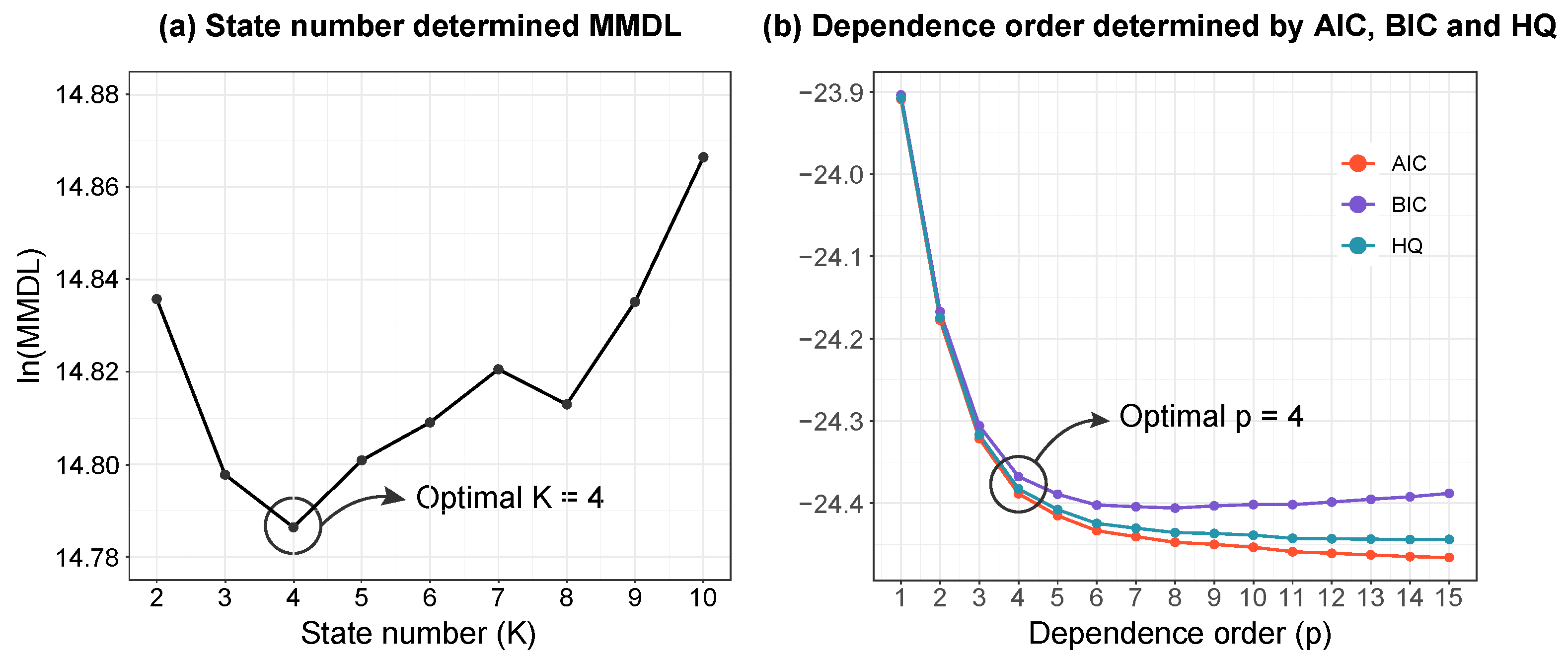
- Fit an AR(p)-HMM to initialize the switching states, and the parameters, . The autoregressive order, p, is determined by AIC, BIC, and HQ criterion;
- To alleviate the possible and undesirable dependence on ordering that arises from the stick-breaking formulation during the inference, we adopt a strategy of greedily fitting a decision list [21] to identify the most suitable permutation of the switching states for the stick-breaking process. Specifically, we start by performing a greedy search on permutations by creating a decision list based on pairs, given bywhere is a permutation of , and are predicates that rely on and provide a true or false. In our framework, these predicates are defined by logistic functions:where should be predetermined. To determine and , we used the maximum a posteriori estimate of the model for each of the K potential states. For the kth logistic regression, the inputs are and the outputs are . We chose the logistic regression model with the largest likelihood as the first output. Then we excluded time points where from the data and proceeded to logistic regressions to predict the subsequent output, , and so on. After cycling through all K results, we obtained the permutation of . In addition, the served as an initialization of the recurrence weights (R).
4. Numerical Experiments
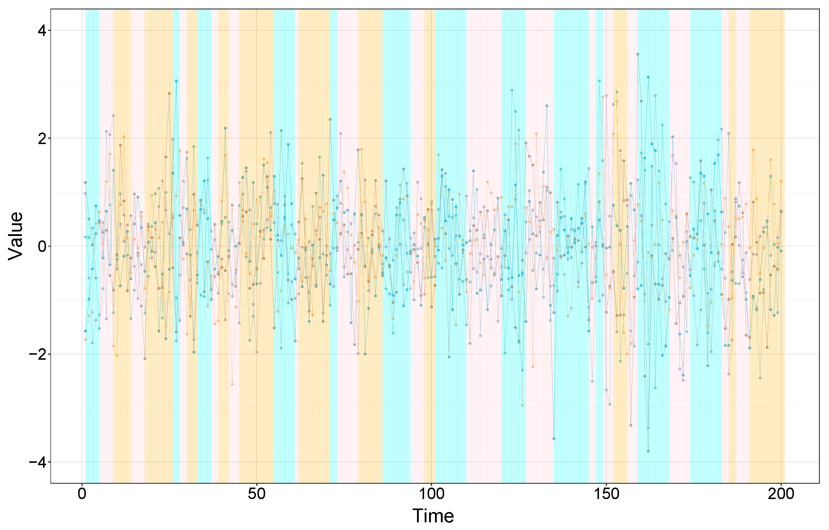
- Benchmark model settings.We take AR-HSMM as a benchmark model to generate synthetic time series. Specifically, the dimensionality of the synthetic time series is , and the total length is . The state number is , and the autoregressive order p takes values .
- Generating . corresponds to the emission parameters involved in the VAR process of latent variables (Equation (11)). The autoregressive coefficient matrices are generated with 50% sparsity (defined as the proportion of the zero elements), i.e., 50% of the elements in are 0. The non-zero elements of are generated to be positive or negative with equal probability, and their absolute value is sampled uniformly between 0.2 and 0.5. The covariance matrices are generated as , with being an orthogonal matrix and assumed positive. The matrix is constructed by orthogonalizing a random matrix whose entries are simulated from a standard Normal, while each is uniformly sampled in the interval . Additionally, a rejection step is done to check that the sampled constituted a stable VAR process.
- Generating switching state sequence . To generate , we set the state transition probabilities to 0.5, for . Note that in an HSMM, the self-transition probability is 0. Furthermore, we simulate the state duration time in two cases. In the first case, the state duration time is sampled from a geometric distribution (the between-state transition probabilities are set to 0.1). In the second case, the state duration time is directly sampled from with specified sampling probabilities. Since the second case does not correspond to a parametric distribution, we denote these two cases as geometric and nonparametric, respectively. In addition, the initial state is uniformly sampled from .
- Generating . corresponds to the emission parameters generating the Gaussian observations (Equation (12)). We generate in the same manner as .
- Repeat the above procedure 100 times to obtain 100 synthetic data by setting different random seeds when generating .
5. Dynamic Functional Connectivity Analysis in fMRI Data
6. Conclusions
Author Contributions
Funding
Data Availability Statement
Conflicts of Interest
Abbreviations
| SLDS | Switching linear dynamical systems |
| HO-SLDS | Switching linear dynamical systems with higher-order dependence |
| HO-rSLDS | Recurrent switching linear dynamical systems with higher-order dependence |
| HMM | Hidden Markov model |
| VAR | Vector autoregressive |
| AR-HMM | Autoregressive hidden Markov model |
| AR-HSMM | Autoregressive hidden semi-Markov model |
| NMSE | Normalized mean squared error |
| SNR | Signal-to-noise ratio |
| fMRI | Functional magnetic resonance imaging |
| DFC | Dynamic functional connectivity |
References
- Fox, E.; Sudderth, E.B.; Jordan, M.I.; Willsky, A.S. Bayesian nonparametric inference of switching dynamic linear models. IEEE Trans. Signal Process. 2011, 59, 1569–1585. [Google Scholar] [CrossRef]
- Pandarinath, C.; O’Shea, D.J.; Collins, J.; Jozefowicz, R.; Stavisky, S.D.; Kao, J.C.; Trautmann, E.M.; Kaufman, M.T.; Ryu, S.I.; Hochberg, L.R.; et al. Inferring single-trial neural population dynamics using sequential auto-encoders. Nat. Methods 2018, 15, 805–815. [Google Scholar] [CrossRef] [PubMed]
- Frigola, R.; Chen, Y.; Rasmussen, C.E. Variational Gaussian process state-space models. In Proceedings of the Annual Conference on Neural Information Processing Systems 2014, Montreal, QC, Canada, 8–13 December 2014; Volume 27. [Google Scholar]
- Krishnan, R.; Shalit, U.; Sontag, D. Structured inference networks for nonlinear state space models. In Proceedings of the AAAI Conference on Artificial Intelligence, San Francisco, CA, USA, 4–9 February 2017; Volume 31. [Google Scholar]
- Hamilton, J.D. Time Series Analysis; Princeton University Press: Princeton, NJ, USA, 2020. [Google Scholar]
- de Souza Baptista, R.; Bó, A.P.; Hayashibe, M. Automatic human movement assessment with switching linear dynamic system: Motion segmentation and motor performance. IEEE Trans. Neural Syst. Rehabil. Eng. 2016, 25, 628–640. [Google Scholar] [CrossRef] [PubMed]
- Liu, H.; Wang, L. Human motion prediction for human-robot collaboration. J. Manuf. Syst. 2017, 44, 287–294. [Google Scholar] [CrossRef]
- Alameda-Pineda, X.; Drouard, V.; Horaud, R.P. Variational inference and learning of piecewise linear dynamical systems. IEEE Trans. Neural Netw. Learn. Syst. 2021, 33, 3753–3764. [Google Scholar] [CrossRef] [PubMed]
- Ma, T.; Srinivasan, S.; Lazarou, G.; Picone, J. Continuous speech recognition using linear dynamic models. Int. J. Speech Technol. 2014, 17, 11–16. [Google Scholar] [CrossRef]
- Pagan, A.R.; Pesaran, M.H. Econometric analysis of structural systems with permanent and transitory shocks. J. Econ. Dyn. Control 2008, 32, 3376–3395. [Google Scholar] [CrossRef]
- Haluszczynski, A.; Räth, C. Controlling nonlinear dynamical systems into arbitrary states using machine learning. Sci. Rep. 2021, 11, 12991. [Google Scholar] [CrossRef] [PubMed]
- Smith, J.F.; Pillai, A.; Chen, K.; Horwitz, B. Identification and validation of effective connectivity networks in functional magnetic resonance imaging using switching linear dynamic systems. Neuroimage 2010, 52, 1027–1040. [Google Scholar] [CrossRef]
- Wang, E.T.; Vannucci, M.; Haneef, Z.; Moss, R.; Rao, V.R.; Chiang, S. A Bayesian switching linear dynamical system for estimating seizure chronotypes. Proc. Natl. Acad. Sci. USA 2022, 119, e2200822119. [Google Scholar] [CrossRef]
- Rabiner, L.R. A tutorial on hidden Markov models and selected applications in speech recognition. Proc. IEEE 1989, 77, 257–286. [Google Scholar] [CrossRef]
- Vidaurre, D. A new model for simultaneous dimensionality reduction and time-varying functional connectivity estimation. PLoS Comput. Biol. 2021, 17, e1008580. [Google Scholar] [CrossRef] [PubMed]
- Hamada, R.; Kubo, T.; Ikeda, K.; Zhang, Z.; Shibata, T.; Bando, T.; Hitomi, K.; Egawa, M. Modeling and prediction of driving behaviors using a nonparametric Bayesian method with AR models. IEEE Trans. Intell. Veh. 2016, 1, 131–138. [Google Scholar] [CrossRef]
- Houpt, J.W.; Frame, M.E.; Blaha, L.M. Unsupervised parsing of gaze data with a beta-process vector auto-regressive hidden Markov model. Behav. Res. Methods 2018, 50, 2074–2096. [Google Scholar] [CrossRef] [PubMed]
- Vidaurre, D.; Quinn, A.J.; Baker, A.P.; Dupret, D.; Tejero-Cantero, A.; Woolrich, M.W. Spectrally resolved fast transient brain states in electrophysiological data. Neuroimage 2016, 126, 81–95. [Google Scholar] [CrossRef] [PubMed]
- Glennie, R.; Adam, T.; Leos-Barajas, V.; Michelot, T.; Photopoulou, T.; McClintock, B.T. Hidden Markov models: Pitfalls and opportunities in ecology. Methods Ecol. Evol. 2023, 14, 43–56. [Google Scholar] [CrossRef]
- Johnson, M.J.; Willsky, A.S. Bayesian Nonparametric Hidden Semi-Markov Models. J. Mach. Learn. Res. 2013, 14, 673–701. [Google Scholar]
- Linderman, S.W.; Johnson, M.J.; Miller, A.C.; Adams, R.P.; Blei, D.M.; Paninski, L. Bayesian Learning and Inference in Recurrent Switching Linear Dynamical Systems. In Proceedings of the 20th International Conference on Artificial Intelligence and Statistics (AISTATS), Fort Lauderdale, FL, USA, 20–22 April 2017; Volume 54, pp. 914–922. [Google Scholar]
- Polson, N.G.; Scott, J.G.; Windle, J. Bayesian inference for logistic models using Pólya–Gamma latent variables. J. Am. Stat. Assoc. 2013, 108, 1339–1349. [Google Scholar] [CrossRef]
- Jacobs, W.R.; Baldacchino, T.; Dodd, T.; Anderson, S.R. Sparse Bayesian nonlinear system identification using variational inference. IEEE Trans. Autom. Control 2018, 63, 4172–4187. [Google Scholar] [CrossRef]
- Yu, S.Z. Hidden semi-Markov models. Artif. Intell. 2010, 174, 215–243. [Google Scholar] [CrossRef]
- Liu, Q.; Liu, W.; Dong, M.; Li, Z.; Zheng, Y. Residual useful life prognosis of equipment based on modified hidden semi-Markov model with a co-evolutional optimization method. Comput. Ind. Eng. 2023, 182, 109433. [Google Scholar] [CrossRef]
- Särkkä, S.; Svensson, L. Bayesian Filtering and Smoothing; Cambridge University Press: Cambridge, UK, 2023; Volume 17. [Google Scholar]
- Tipping, M.E.; Bishop, C.M. Probabilistic principal component analysis. J. R. Stat. Soc. Ser. B Stat. Methodol. 1999, 61, 611–622. [Google Scholar] [CrossRef]
- Glasser, M.F.; Sotiropoulos, S.N.; Wilson, J.A.; Coalson, T.S.; Fischl, B.; Andersson, J.L.; Xu, J.; Jbabdi, S.; Webster, M.; Polimeni, J.R.; et al. The minimal preprocessing pipelines for the Human Connectome Project. Neuroimage 2013, 80, 105–124. [Google Scholar] [CrossRef] [PubMed]
- Hutchison, R.M.; Womelsdorf, T.; Allen, E.A.; Bandettini, P.A.; Calhoun, V.D.; Corbetta, M.; Della Penna, S.; Duyn, J.H.; Glover, G.H.; Gonzalez-Castillo, J.; et al. Dynamic functional connectivity: Promise, issues, and interpretations. Neuroimage 2013, 80, 360–378. [Google Scholar] [CrossRef] [PubMed]
- Motlaghian, S.; Vahidi, V.; Baker, B.; Belger, A.; Bustillo, J.; Faghiri, A.; Ford, J.; Iraji, A.; Lim, K.; Mathalon, D.; et al. A method for estimating and characterizing explicitly nonlinear dynamic functional network connectivity in resting-state fMRI data. J. Neurosci. Methods 2023, 389, 109794. [Google Scholar] [CrossRef]
- Zhang, G.; Cai, B.; Zhang, A.; Stephen, J.M.; Wilson, T.W.; Calhoun, V.D.; Wang, Y.P. Estimating dynamic functional brain connectivity with a sparse hidden Markov model. IEEE Trans. Med. Imaging 2019, 39, 488–498. [Google Scholar] [CrossRef] [PubMed]
- Barron, A.; Rissanen, J.; Yu, B. The minimum description length principle in coding and modeling. IEEE Trans. Inf. Theory 1998, 44, 2743–2760. [Google Scholar] [CrossRef]
- Gredenhoff, M.; Karlsson, S. Lag-length selection in VAR-models using equal and unequal lag-length procedures. Comput. Stat. 1999, 14, 171–187. [Google Scholar] [CrossRef]
- Brovelli, A.; Ding, M.; Ledberg, A.; Chen, Y.; Nakamura, R.; Bressler, S.L. Beta oscillations in a large-scale sensorimotor cortical network: Directional influences revealed by Granger causality. Proc. Natl. Acad. Sci. USA 2004, 101, 9849–9854. [Google Scholar] [CrossRef]
- Teh, Y.W.; Jordan, M.I.; Beal, M.J.; Blei, D.M. Hierarchical Dirichlet Processes. J. Am. Stat. Assoc. 2006, 101, 1566–1581. [Google Scholar] [CrossRef]


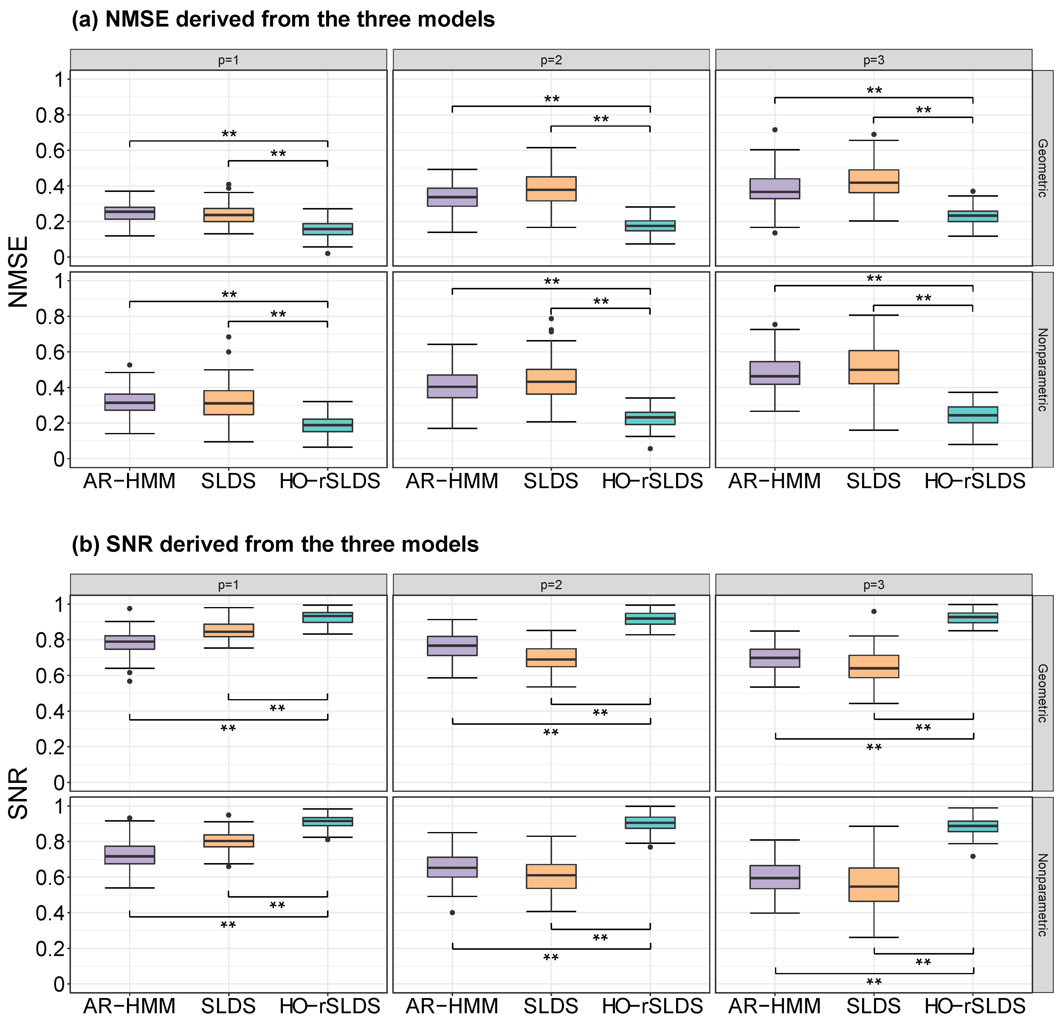
| NMSE | ||||
|---|---|---|---|---|
| Geometric | AR-HMM | 0.25 ± 0.06 | 0.33 ± 0.07 | 0.37 ± 0.09 |
| SLDS | 0.23 ± 0.05 | 0.39 ± 0.09 | 0.44 ± 0.11 | |
| HO-rSLDS | 0.16 ± 0.04 | 0.17 ± 0.05 | 0.20 ± 0.06 | |
| Nonparametric | AR-HMM | 0.32 ± 0.07 | 0.41 ± 0.09 | 0.48 ± 0.11 |
| SLDS | 0.31 ± 0.09 | 0.44 ± 0.11 | 0.49 ± 0.13 | |
| HO-rSLDS | 0.18 ± 0.06 | 0.20 ± 0.05 | 0.21 ± 0.06 | |
| SNR | ||||
|---|---|---|---|---|
| Geometric | AR-HMM | 0.79 ± 0.08 | 0.76 ± 0.07 | 0.69 ± 0.08 |
| SLDS | 0.85 ± 0.06 | 0.68 ± 0.09 | 0.64 ± 0.09 | |
| HO-rSLDS | 0.93 ± 0.04 | 0.92 ± 0.05 | 0.90 ± 0.05 | |
| Nonparametric | AR-HMM | 0.73 ± 0.08 | 0.65 ± 0.07 | 0.59 ± 0.10 |
| SLDS | 0.80 ± 0.06 | 0.60 ± 0.09 | 0.54 ± 0.11 | |
| HO-rSLDS | 0.91 ± 0.04 | 0.87 ± 0.05 | 0.86 ± 0.05 | |
Disclaimer/Publisher’s Note: The statements, opinions and data contained in all publications are solely those of the individual author(s) and contributor(s) and not of MDPI and/or the editor(s). MDPI and/or the editor(s) disclaim responsibility for any injury to people or property resulting from any ideas, methods, instructions or products referred to in the content. |
© 2024 by the authors. Licensee MDPI, Basel, Switzerland. This article is an open access article distributed under the terms and conditions of the Creative Commons Attribution (CC BY) license (https://creativecommons.org/licenses/by/4.0/).
Share and Cite
Wang, H.; Chen, J. Bayesian Inference of Recurrent Switching Linear Dynamical Systems with Higher-Order Dependence. Symmetry 2024, 16, 474. https://doi.org/10.3390/sym16040474
Wang H, Chen J. Bayesian Inference of Recurrent Switching Linear Dynamical Systems with Higher-Order Dependence. Symmetry. 2024; 16(4):474. https://doi.org/10.3390/sym16040474
Chicago/Turabian StyleWang, Houxiang, and Jiaqing Chen. 2024. "Bayesian Inference of Recurrent Switching Linear Dynamical Systems with Higher-Order Dependence" Symmetry 16, no. 4: 474. https://doi.org/10.3390/sym16040474
APA StyleWang, H., & Chen, J. (2024). Bayesian Inference of Recurrent Switching Linear Dynamical Systems with Higher-Order Dependence. Symmetry, 16(4), 474. https://doi.org/10.3390/sym16040474