Cascading Failure Modeling for Circuit Systems Considering Continuous Degradation and Random Shocks Using an Impedance Network

Abstract

The reliability of circuit systems is primarily affected by cascading failures due to their complex structural and functional coupling. Causes of cascading failure during circuit operation include the continuous degradation process of components and external random shocks. Circuit systems can exhibit asymmetric structural changes and functional loss during cascading failure propagation due to the coupling of degradation and shock and their uncertainty effects. To tackle this issue, this paper abstracts the circuit into an impedance network and constructs a component failure behavior model that considers the correlation between degradation and shock. The interactions between soft and hard failure processes among different components are discussed. Two types of cascading failure propagation processes are described: slow propagation associated with continuous degradation and damage shock, and fast propagation due to fatal shock. Based on this, a cascading failure simulation algorithm is developed. This article presents a case study to demonstrate the proposed models and to analyze the reliability of a typical circuit system.

1. Introduction

Circuits are defined as closed-loop or open-loop systems of discrete components that perform a specific function [1]. Their failure can pose a serious threat to the safety of equipment and even personnel [2]. Cascading failures are a major cause of circuit reliability as the circuit scale increases, due to structural and functional coupling. This failure process is characterized by the redistribution of current resulting from the failure of one or several components. This, in turn, triggers the overload failure of other components and ultimately leads to the collapse of the circuit as a whole [3,4]. The current redistribution process within the circuit is global, which can result in asymmetric failure propagation paths and uncertainty in failure times due to continuous degradation and random shocks.

The methods for traditional circuit failure analysis can be classified into two categories: failure logic-based [5,6,7] and system simulation-based [8,9]. The former analyzes the correlation and impact of component failures and determines the root causes of system failure using methods such as decision trees [5], fault propagation directed graphs [6], and Petri nets [7]. The latter method analyzes the impact of component failure on the system response by constructing circuit system performance simulation models and combining them with component failure mechanism models. Although these two methods describe the correlation problem between failures within the circuit to some extent, they also have their own limitations. The failure logic-based method relies mainly on the engineering experience of designers, which is difficult to quantitatively describe. As the system size increases, the circuit system state shows an exponential explosion, making it increasingly difficult to meet the actual analysis needs [10]. The system simulation-based method can reflect changes in the input state of internal components in the output response of the circuit. However, it cannot characterize the propagation of failure through the system, making it difficult to identify the intrinsic law of system cascading failure.

In recent years, a network-based approach has been proposed to model cascading failures in circuits, in order to overcome the shortcomings of traditional methods. This approach abstracts the circuit system into a network topology and analyzes the inherent cascading failure propagation behavior of the circuit. Depending on the type of loads and solution methods, network-based methods can be categorized into three types: topological models [11,12,13], analytical equation-based models [14,15,16], and redistribution factor models [3,4]. Topological models concentrate on the correlation between pure topological parameters, such as clustering coefficients [11,12] and betweenness [13], and cascading failures. However, they neglect the physical laws governing the transfer of circuit current loads. This can result in significant differences in describing the propagation behavior of cascading failures. Analytical equation-based models are proposed to take into account both topological and physical parameters. The redistributed currents of the failed components are obtained by directly or indirectly solving Kirchhoff’s and Ohm’s laws [14,15,16]. However, this approach is similar to traditional simulation methods and does not account for the correlation between components, as well as being computationally expensive. In contrast, the redistribution factor model combines the network topology and physical laws to derive a current redistribution factor that describes the effect of failed or degraded components on the remaining component currents [3,4,17,18,19]. This method clarifies the correlation between components and is computationally efficient. However, it only considers the cascading propagation process under degradation or sudden failure. In the real operating environment of a circuit, cascading failure is often triggered by the coexistence of degradation and shock. Therefore, the redistribution factor model needs further investigation to more accurately reflect circuit failure behavior.

Currently, research on degradation and shock correlation focuses on multi-component systems. The interrelationships of degradation and shock, such as competition and accumulation [20,21,22,23], are discussed at the component level. The reliability model of multi-component systems is constructed by mainly considering the mutual effects of soft and hard failures of different components subject to degradation and shock at the system level [24,25,26,27]. However, this modeling is only applicable to simple systems that can provide structure functions. Constructing an accurate structure–function that quantifies the relationship between components and systems can be challenging, particularly for complex systems such as circuit systems. Furthermore, due to the presence of failure correlation, assuming independence based on the failure of the component does not accurately describe the failure behavior of the entire circuit system. Modeling the propagation of cascading failures presents three main challenges. Firstly, it is necessary to describe the correlation between the failure processes caused by the degradation and shock of individual components. Secondly, it is important to consider the interactions between these two types of failure processes among different components. Finally, it is necessary to describe the cascading failure propagation behavior of the circuit system, taking into account the combined effects of degradation and shock.

To handle the above problems, this paper aims to characterize the cascading failure behavior under degradation–shock effects. It begins at the component level, discussing the relevance of the failure process of individual components under degradation and shock coupling, as well as their interactions among different components. From this, circuit failure triggering conditions are identified, and the dynamic propagation behavior of the circuit system under degradation and shock effects is described in conjunction with a current redistribution factor model. The main technical contributions of this paper are summarized as follows:

• This paper presents a failure model for components that takes into account the correlation between degradation and shock. Additionally, it provides a spatio-temporal method for determining cascading failure in combination with the competitive failure model.
• This paper proposes a cascading failure model for circuits that considers the coupling between degradation and shock. The model can take into account asymmetric failure propagation paths and failure time distributions for circuits affected by degradation–shock coupling and its uncertainties.

The rest of this article is organized as follows: Section 2 briefly describes the abstraction of a circuit system into an impedance network. A component failure model considering degradation–shock correlation is built in Section 3. Section 4 presents the cascading failure model with two dynamic propagation models: slow and fast. Additionally, a simulation algorithm is also proposed in this section. In Section 5, a prototype circuit system is built to analyze the cascading failure behavior with degradation and shock. Finally, Section 6 concludes this article.

2. System Description

2.1. Circuit as an Impedance Network

This paper focuses on a basic circuit system without the nonlinear characteristics of passive devices and the control effects of active devices. Specifically, we assume that the basic circuit only consists of components that can be described as impedances, such as resistance, capacitance, and inductance. In this sense, the impedance network is utilized as a tool to model the circuit system.

The impedance network can be viewed as an undirected weighted graph $Graph=g\left(V,L\right)$. In the circuit system, the components are represented as the edges in $L=\left\{ij\left|i,j\in V,i\ne j\right.\right\}$ and the electrical connections between components are described by the nodes in $V=\left\{1,2,\dots ,v\right\}$. The impedances of the components that reflect the difficulty of current to flow through the network are defined as the weight of edge ij, denoted by $Z_{ij}$. The circuit’s power is divided into two virtual nodes: the source node, where the current flows into the network, and the sink node, where the current flows out of the network. The connection relationship among nodes can be described by the adjacency matrix A. If there is an electrical connection between node i and node j, then $a_{ij}=1$; otherwise, $a_{ij}=0$. Therefore, the impedance network can be clearly established based on the above representation.

2.2. Basic Modeling Methods

During circuit operation, degradation and shock act together on individual components and trigger component failures to propagate cascading failures through the system. Therefore, we intend to construct the model from two aspects.

(1)

At the component level, we focus mainly on the mutual influence of degradation and shock on individual components and the competition between different components. In this sense, the modeling methods include the following:

• Describe the weakening effect of continuous degradation on shock thresholds (Equation (13)) and the accelerating effect of damage shocks on impedance degradation (Equation (5)) (see Section 3.1);
• Using competitive failure models to determine whether a component undergoes soft failure dominated by degradation or hard failure dominated by fatal shock (see Section 3.3).

(2)

At the system level, we need to reveal the cascading failure propagation mechanisms and quantify the propagation process. In this regard, the modeling methods of this paper are the following:

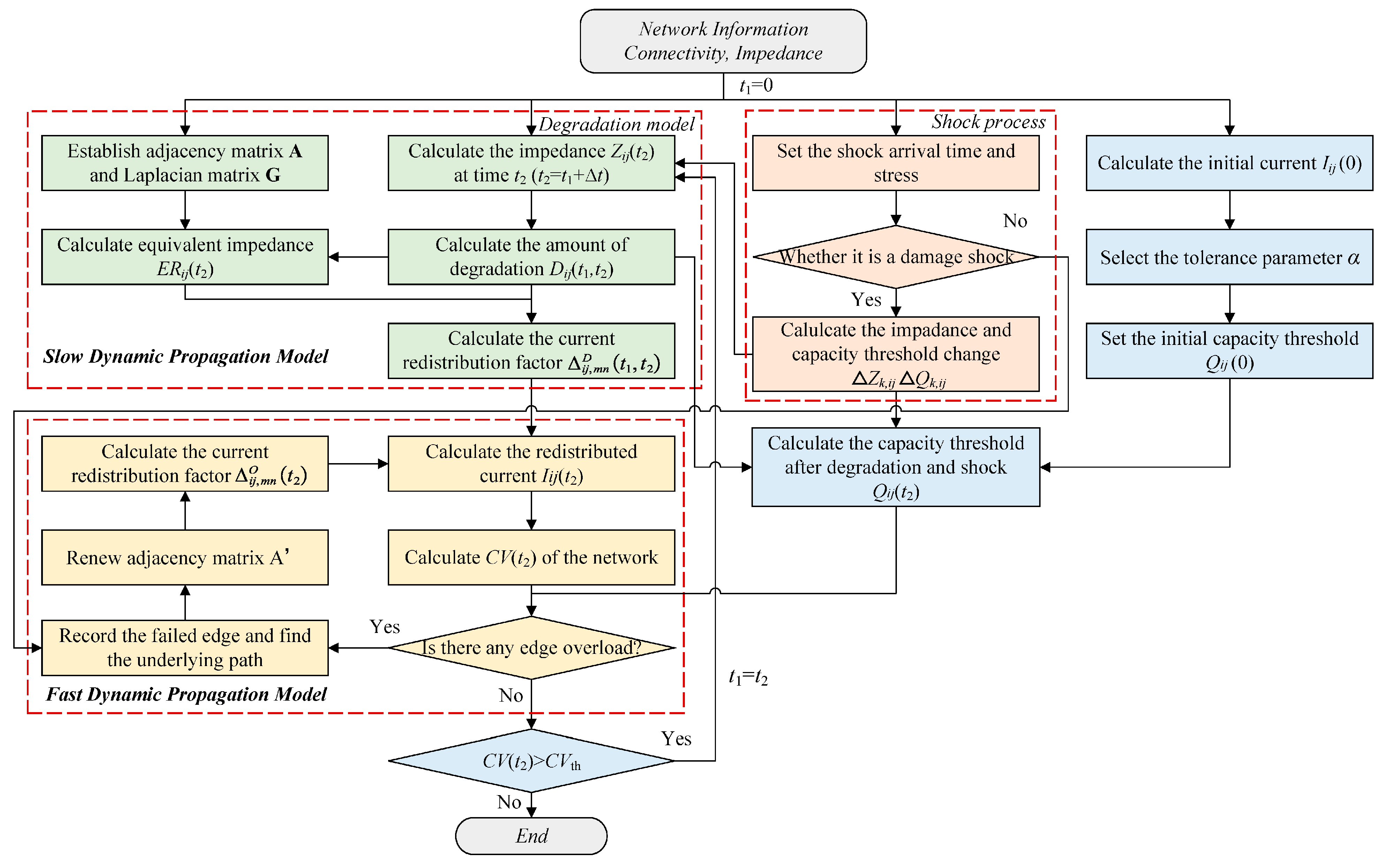
• Divide the failure propagation process into two distinct processes: a slow propagation process, where cascading failure is not triggered by continuous degradation and damage shock, and a fast propagation process, where cascading failure is triggered by any component failure (see Section 4.1);
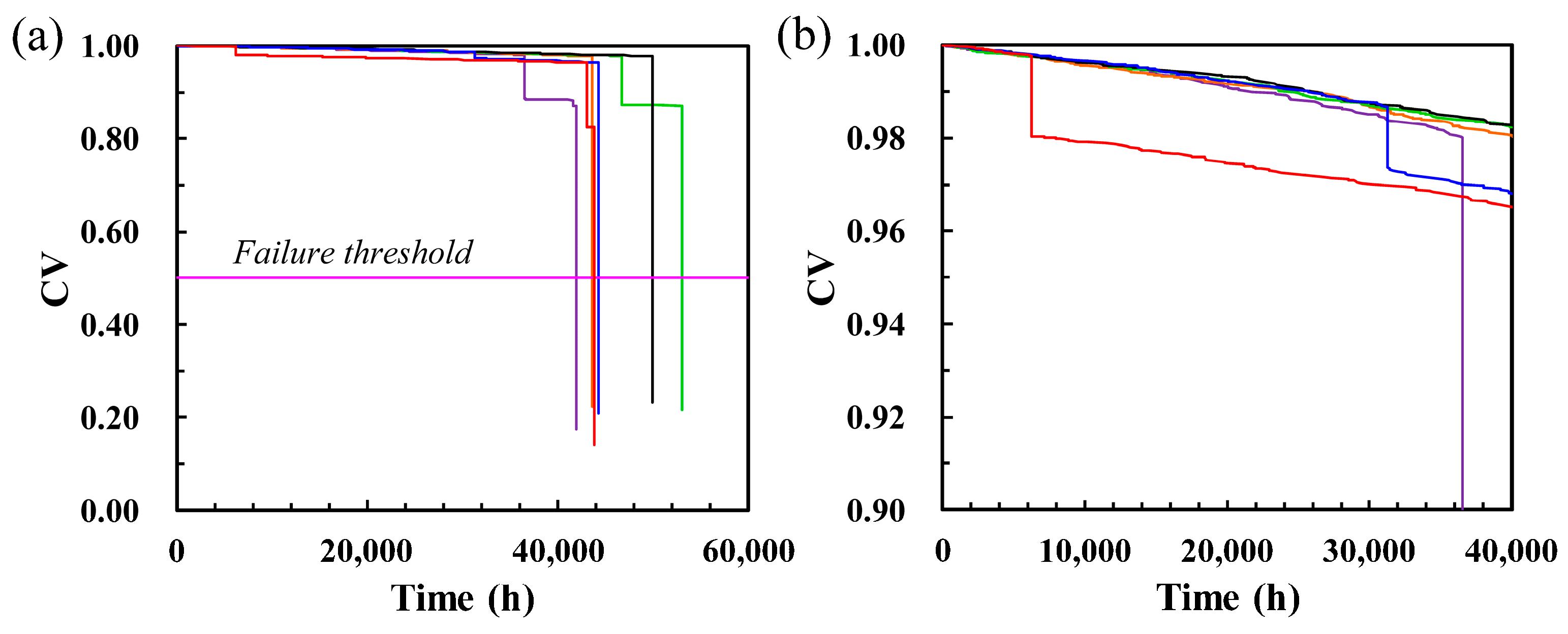
• Propose a health confidence value from both structural and functional perspectives to assess the cascading failure propagation process of the system under degradation and shocks (see Section 4.2).

3. Component Failure Modeling Considering Degradation–Shock Correlation

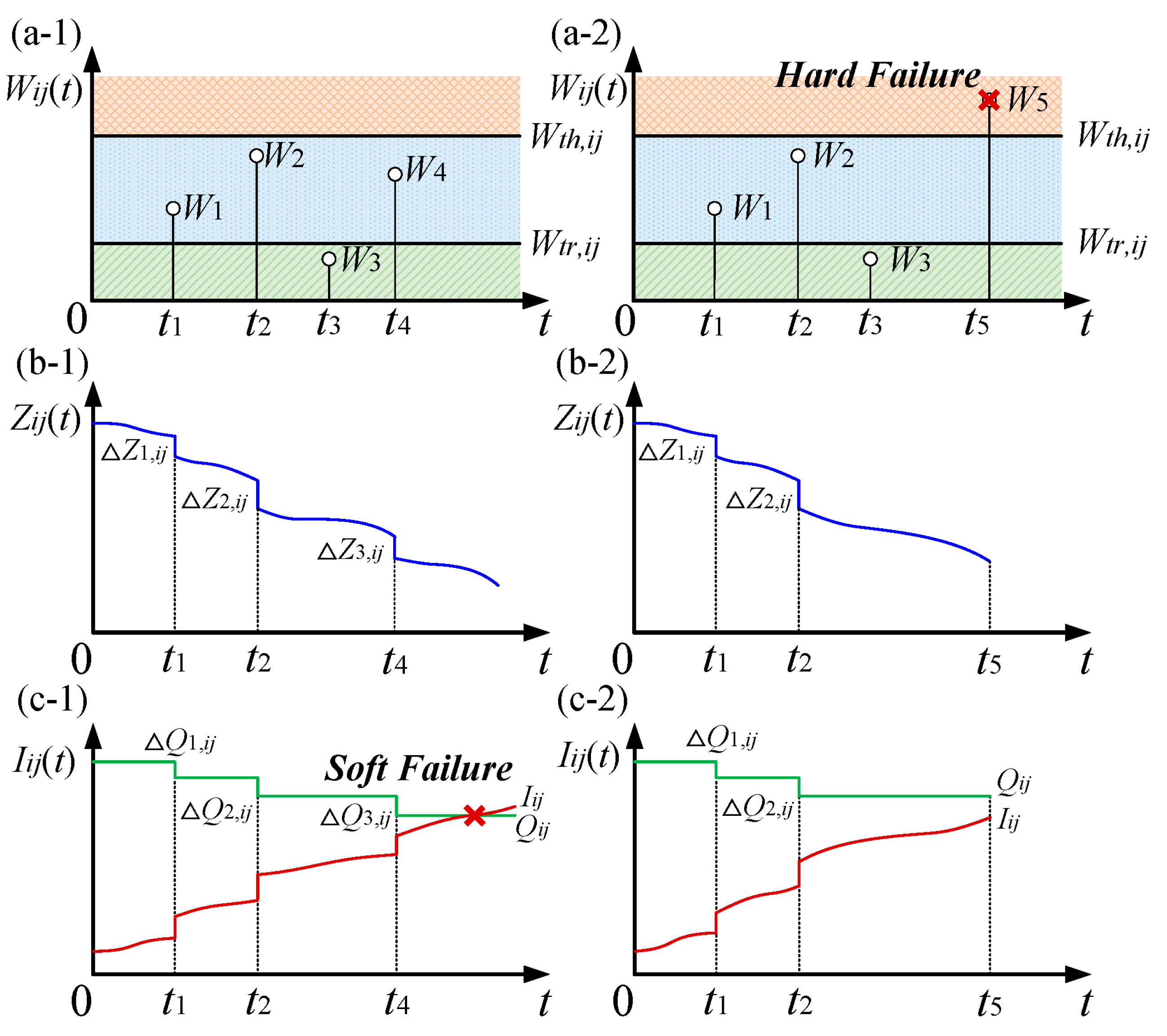
3.1. Component-Triggered Failure Conditions

This paper assumes that the effects of degradation and shock lead to two types of failure processes in components: soft failure and hard failure processes.

As shown in Figure 1a, random shocks affect both types of failure processes depending on the magnitude of the shock stress. If the shock stress $W_k$ exceeds the strength threshold $W_{th}$, it leads directly to transient failure of the component, resulting in hard failure. However, if the shock stress $W_k$ is below the strength threshold $W_{th}$, a single shock will not cause direct failure of the component. Instead, it will lead to damage accumulation in the component and affect the continuous degradation process.

Component degradation is usually identified by changes in impedance. This process leads to the redistribution of the current across the circuit’s components. Soft failure occurs when the current flowing through the component exceeds its capacity threshold.

Therefore, cascading failure can be triggered when either of the above two types of failure occurs in the component ij, as follows:

• Hard failure occurs when the stress $W_{k,ij}$ of the kth shock exceeds the strength threshold $W_{th,ij}$ during random shocks, as shown in Figure 1(a-2);
• Soft failure occurs when the redistributed current $I_{ij}\left(t\right)$ on the component ij, subjected to continuous degradation (including damage shocks during random shocks), is greater than its own capacity threshold $Q_{ij}\left(t\right)$, as shown in Figure 1(c-1).

3.2. Degeneration–Shock Process Assumptions

In order to reveal the failure behavior of components, this paper proposes the following assumptions for the continuous degradation process, the stochastic shock process, and the correlation between them.

Assumption 1. 

The random shock originates from the external environment, and the circuit system does not affect the frequency of the shock. It is assumed that the random shock follows a homogeneous Poisson process with intensity $\lambda$, i.e., $\left\{N\left(t\right),t\ge 0\right\}$. Then, the sequence of intervals of shock arrivals $\left\{T_n\left(t\right),n>0\right\}$ is independently and identically distributed and obeys an exponential distribution with mean $1/\lambda$. The number $N\left(t\right)$ of shock arrivals in the $\left(0,t\right]$ interval follows a Poisson distribution with mean $\lambda t$:

$$P\left(N\left(t\right)=n\right)=\frac{e^{-\lambda t}{\left(\lambda t\right)}^n}{n!}.$$

(1)

Assumption 2. 

According to the level of impact on components, shock stresses are classified into three categories by setting strength thresholds $W_{th}$ and trigger thresholds $W_{tr}$: fatal shock ($W_k>W_{th}$), damage shock ($W_{th}>W_k>W_{tr}$), and safety shock ($W_k<W_{tr}$). It is assumed that each shock stress $W_k$ in the random shock process is a set of independent and identically distributed random variables. The probability of a shock stress belonging to one of the three types of shocks is $P_1$, $P_2$, or $P_3$, respectively.

According to Assumption 1, the above three types of shocks are non-homogeneous Poisson processes. The intensities of these processes are denoted by $P_1\left(t\right)\lambda$, $P_2\left(t\right)\lambda$, and $P_3\left(t\right)\lambda$, respectively. The probabilities $P_1\left(t\right)$, $P_2\left(t\right)$, and $P_3\left(t\right)$ are affected by the strength thresholds $W_{th}\left(t\right)$ and trigger thresholds $W_{tr}\left(t\right)$ with time t.

Assumption 3. 

For any component ij, the damage shock mainly affects the continuous degradation process, which is reflected in two ways. Firstly, the damage shock leads to a transient change in component impedance. Assuming that the impedance change $\mathsf{\Delta }{Z}_{k,ij}$ caused by the damage shock is proportional to the shock stress $W_{k,ij}$, i.e., $\mathsf{\Delta }{Z}_{k.ij}=\zeta W_{k,ij}$, and $\zeta$ represents the impedance degradation coefficient. Secondly, the damage shock reduces the component’s ability to resist current overload, resulting in a decrease in the capacity threshold $Q_{ij}$. It is assumed that the change $\mathsf{\Delta }{Q}_{k,ij}$ in the capacity threshold caused by each damage shock is proportional to the shock stress $W_{k,ij}$; that is, $\mathsf{\Delta }{Q}_{k,ij}=\eta W_{k,ij}$, and $\eta$ is the capacity degradation coefficient.

Assumption 4. 

The effect of degradation on shock is evident in the change in strength threshold $W_{th,ij}$. As component degradation $D_{ij}\left(t\right)$ increases, the strength threshold $W_{th,ij}$ decreases, increasing the probability $P_1\left(t\right)$ of a fatal shock and decreasing the probability $P_2\left(t\right)$ of a damage shock. Additionally, the trigger threshold remains constant, resulting in an unchanged probability $P_3\left(t\right)$ of a safety shock. This relationship is expressed as follows:

$$P_1\left(t\right)=\mathrm{Pr}\left\{W_{k,ij}>W_{th,ij}\left(1-D_{ij}\left(t\right)\right)\right\},$$

(2)

$$P_2\left(t\right)=\mathrm{Pr}\left\{W_{th,ij}\left(1-D_{ij}\left(t\right)\right)>W_{k,ij}>W_{tr,ij}\right\}.$$

(3)

3.3. Component Failure Model

Based on the above assumptions, the soft and hard failure processes of any component ij are modeled separately.

3.3.1. Hard Failure Model

Hard failure occurs when the shock stress $W_{k.ij}$ exceeds the strength threshold $W_{th,ij}$. According to the assumption of random shock classification, the hard failure occurrence time $T_{1,ij}$ is equivalent to the time when the first fatal shock is reached. This can be expressed as the following:

$$T_{1,ij}=\inf \left\{t\left|W_{k,ij}\left(t\right)>W_{th,ij}\right.\right\}.$$

(4)

3.3.2. Soft Failure Model

Soft failures occur when continuous degradation and damage shocks cause redistributed currents $I_{ij}\left(t\right)$ in component ij that exceed their capacity thresholds $Q_{ij}\left(t\right)$.

First, the effect of these factors on the current is reflected in the change in impedance. The affected impedance $Z_{ij}^S\left(t\right)$ can be described by the component’s degradation model $Z_{ij}\left(t\right)$ and the cumulative amount of impedance change $S_{ij}\left(t\right)$ caused by damage shocks, which can be expressed as follows:

$$Z_{ij}^S\left(t\right)=Z_{ij}\left(t\right)+S_{ij}\left(t\right)$$

(5)

According to ref. [3], the degradation modeling for resistors and capacitors can be expressed as follows:

$$\frac{R\left(t\right)}{R_0}={\alpha }_1{t}^{\beta }\exp \left(-\frac{E_{A,1}}{kT}\right)+{\sigma }_{1}B\left(t\right),$$

(6)

$$\frac{C\left(t\right)}{C_0}={\alpha }_{2}t\exp \left(-\frac{E_{A,2}}{kT}\right)+{\sigma }_{2}B\left(t\right),$$

(7)

where $R\left(t\right)$ and $C\left(t\right)$ are the resistance and the capacitance at moment t, $R_0$ and $C_0$ are the initial values of resistance and capacitance, $E_{A,1}$ and $E_{A,2}$ are the activation energy of resistance and capacitance, T is the temperature, $\beta$ is the time coefficient, ${\alpha }_1$ and ${\alpha }_2$ are pre-exponential constant characteristic, ${\sigma }_1$ and ${\sigma }_2$ are the diffusion coefficients, and $B\left(t\right)$ is the standard Brownian motion with $B\left(t\right)\sim N\left(0,t\right)$.

$S_{ij}\left(t\right)$ is related to the number and stress of random damage shocks, which can be described by a cumulative damage shock model, i.e.,

$$S_{ij}\left(t\right)=\left\{\begin{array}{cc}{\displaystyle \sum _{k=1}^{N_2\left(t\right)}\mathsf{\Delta }{Z}_{k,ij}}={\displaystyle \sum _{i=1}^{N_2\left(t\right)}\zeta W_{k,ij}}& N_2\left(t\right)>0\\ 0& N_2\left(t\right)=0\end{array}\right.$$

(8)

Since the random damage shock $\left\{N_2\left(t\right),t\ge 0\right\}$ is a non-homogeneous Poisson process obeying the intensity of $P_2\left(t\right)\lambda$, the probability distribution function of $N_2\left(t\right)$ is

$$P\left(N_2\left(t\right)=n\right)=\frac{e^{-\lambda a_2\left(t\right)}{\left(\lambda a_2\left(t\right)\right)}^n}{n!},$$

(9)

where $a_2\left(t\right)={\displaystyle {\int }_0^t{P}_2\left(u\right)}du$.

The impedance change due to degradation from time t₁ and t₂ can be characterized as $Z_{ij}^S\left(t_2\right)={\varphi }_{ij}^S\left(t_1,t_2\right)Z_{ij}^S\left(t_1\right)$, where ${\varphi }_{ij}^S\left(t_1,t_2\right)$ is a degradation coefficient and calculated by

$${\varphi }_{ij}^S\left(t_1,t_2\right)=\left\{\begin{array}{ll}1+D_{ij}\left(t_1,t_2\right),& if\hspace{0.33em}edge\hspace{0.33em}ij\hspace{0.33em}is\hspace{0.33em}\mathit{resitance}\\ \frac{1}{1+D_{ij}\left(t_1,t_2\right)},& if\hspace{0.33em}edge\hspace{0.33em}ij\hspace{0.33em}is\hspace{0.33em}\mathit{capacitance}\end{array}\right.$$

(10)

Based on the derivation in ref. [3], the redistributed current of component ij due to global degradation can be expressed as follows:

$$I_{ij}\left(t_2\right)=I_{ij}\left(t_1\right)\left(1-{\displaystyle \sum _{mn\in edge\backslash \left\{ij\right\}}{\mathsf{\Delta }}_{mn,ij}^D\left(t_1,t_2\right)}\right)+{\displaystyle \sum _{mn\in edge\backslash \left\{ij\right\}}{I}_{mn}\left(t_1\right){\mathsf{\Delta }}_{ij,mn}^D\left(t_1,t_2\right)},$$

(11)

where ${\mathsf{\Delta }}_{mn,ij}^D\left(t_1,t_2\right)$ (or ${\mathsf{\Delta }}_{ij,mn}^D\left(t_1,t_2\right)$) are the current redistribution factors that reflect the influence of the degraded component mn (or component ij) on the current flowing through the component ij (or component mn).

The current redistribution factor ${\mathsf{\Delta }}_{mn,ij}^D\left(t_1,t_2\right)$ can be calculated by

$${\mathsf{\Delta }}_{ij,mn}^D\left(t_1,t_2\right)=\frac{\left[E{R}_{in}^S\left(t_2\right)-E{R}_{im}^S\left(t_2\right)+E{R}_{jm}^S\left(t_2\right)-E{R}_{jn}^S\left(t_2\right)\right]\left[{\varphi }_{mn}^S\left(t_1,t_2\right)-1\right]Z_{mn}^S\left(t_2\right)}{\left[E{R}_{mn}^S\left(t_2\right)-Z_{mn}^S\left(t_2\right)\right]{\varphi }_{mn}^S\left(t_1,t_2\right)Z_{ij}^S\left(t_2\right)},$$

(12)

where $E{R}_{ij}^S$ denotes the two-point equivalent impedance between two arbitrary nodes i and j, according to ref. [28].

According to Assumption 3, the capacity threshold $Q_{ij}\left(t\right)$ under $N_2\left(t\right)$ damage shocks at time t can be expressed as follows:

$$Q_{ij}\left(t\right)=\left\{\begin{array}{cc}{Q}_{ij}\left(0\right)-{\displaystyle \sum _{k=1}^{N_2\left(t\right)}\eta W_{k,ij},}& N_2\left(t\right)>0\\ Q_{ij}\left(0\right),& N_2\left(t\right)=0\end{array}\right.$$

(13)

where $Q_{ij}\left(0\right)$ is the initial capacity threshold, proportional to the initial current $I_{ij}\left(0\right)$, i.e., $Q_{ij}\left(0\right)=\left(1+\tau \right)I_{ij}\left(0\right)$, and $\tau$ is the tolerance parameter.

Therefore, the soft failure occurrence time $T_{2,ij}$ can be calculated by the stress-strength model, i.e.,

$$T_{2,ij}=\inf \left\{t\left|I_{ij}\left(t\right)>Q_{ij}\left(t\right)\right.\right\}.$$

(14)

3.3.3. Coupling Model

For a single component, there is a competing failure relationship between the two types of failure processes, and it can be assumed that the failure time $T{F}_{ij}$ of the component is determined by the minimum of the hard failure occurrence time $T_{1,ij}$ and the soft failure occurrence time $T_{2,ij}$, i.e.,

$$T{F}_{ij}=\min \left\{T_{1,ij},T_{2,ij}\right\}.$$

(15)

For the circuit system, the component with the smallest failure time $T{F}_{ij}$ is the first to be triggered, and inter-component failures still follow a competitive relationship:

$$T{F}_{sys}=\min \left\{T{F}_{ij}\right\},ij\in \mathrm{remian},\mathrm{edge}.$$

(16)

4. Cascading Failure Modeling

The network cascading failure process can be described by two dynamic propagation models, slow and fast, due to the continuous effect of component degradation and the transient nature of random shocks. The two models are constructed separately in this section. Furthermore, an algorithm is proposed to simulate the spatial and temporal evolution of failure propagation, while adopting a health confidence value to quantify the overall health state of the impedance network.

4.1. Dynamic Propagation Model

4.1.1. Slow Dynamic Propagation Model

The slow dynamic propagation model explains how the impedance, current, and failure threshold of components in an impedance network change over time due to continuous degradation and random damage shocks, without experiencing soft or hard failures.

The current redistribution process can be described by Equation (11), wherein ${\mathsf{\Delta }}_{mn,ij}^D(t_1,t_2)$ represents the interaction between the components in the network, considering their respective degradations and shocks. The capacity threshold reduction process can be calculated by Equation (13). Furthermore, the trigger condition for hard failure is the arrival of the first fatal shock, which can be expressed by Equation (4).

Based on this, it is noted that the component will be triggered to failure whenever the current I_ij(t) on the component ij exceeds its own capacity threshold Q_ij(t) or the shock stress W_k,ij is greater than the strength threshold W_th,ij. Therefore, an indicator function is proposed to describe the state of each component ij due to continuous degradation and random damage shocks in the following form:

$$P_{ij}=\left\{\begin{array}{ll}1,& if\left\{I_{ij}\left(t\right)\ge Q_{ij}\left(t\right)\right\}\cup \left\{W_{k,ij}\ge W_{th,ij}\right\}\\ 0,& if\left\{I_{ij}\left(t\right)<Q_{ij}\left(t\right)\right\}\cap \left\{W_{k,ij}<W_{th,ij}\right\}\end{array}\right.$$

(17)

For all the components of the impedance network, once $\exists mn\in L$ with $P_{mn}=1$, then the impedance network enters the fast dynamic cascading failure propagation process. Otherwise, the impedance network remains in the slow dynamic propagation process.

4.1.2. Fast Dynamic Propagation Model

When a component triggers a soft or hard failure due to degradation–shock effects, the cascading failure will propagate rapidly within the network. This paper assumes that the failure mode caused by overload due to degradation is open-circuit failure. Therefore, the fast dynamic propagation model is similar to the cascading failure propagation process described in refs. [3,4]. Additionally, the disconnection of component mn will further trigger the redistribution of current on the remaining components. This process can be described by a current redistribution factor ${\mathsf{\Delta }}_{ij,mn}^O\left(t^{-}\right)$ for an open circuit.

$$I_{ij}\left(t^{+}\right)=I_{ij}\left(t^{-}\right)+I_{mn}\left(t^{-}\right){\mathsf{\Delta }}_{ij,mn}^O\left(t^{-}\right)$$

(18)

$${\mathsf{\Delta }}_{ij,mn}^O\left(t^{-}\right)=\frac{\left[E{R}_{in}^S\left(t^{-}\right)-E{R}_{im}^S\left(t^{-}\right)+E{R}_{jm}^S\left(t^{-}\right)-E{R}_{jn}^S\left(t^{-}\right)\right]Z_{mn}^S\left(t^{-}\right)}{2\left[Z_{mn}^S\left(t^{-}\right)-E{R}_{mn}^S\left(t^{-}\right)\right]Z_{ij}^S\left(t^{-}\right)}$$

(19)

where t⁻ and t⁺ represent the moment before and after the open circuit of component mn. If the redistributed current of a component exceeds its capacity threshold, the component is further removed and the redistributed current is recalculated using Equation (18). The cascading failure only stops when all remaining components have currents below their capacity threshold, and the slow dynamic propagation process resumes.

4.2. Health Status of the Impedance Network

In this paper, the impedance network state during cascading failure propagation is measured in terms of the structural integrity index $S_{sys}\left(t\right)$ and functional availability index $E_{sys}\left(t\right)$, respectively. Based on this, a health confidence value $CV\left(t\right)$ is further adopted to evaluate the health state comprehensively, which is expressed as [3,4]

$$CV\left(t\right)=\gamma E_{sys}\left(t\right)+\delta S_{sys}\left(t\right)\left(\gamma +\delta =1,0\le \gamma ,\delta \le 1\right),$$

(20)

$$S_{sys}\left(t\right)={\left(\frac{N_{total}-N_{fail}\left(t\right)}{N_{total}}\right)}^3,$$

(21)

$$E_{sys}\left(t\right)=\frac{1}{N_{remain}\left(t\right)}{\displaystyle \sum _{ij\in \left\{edge,remain\right\}}\left(1-\frac{\left|I_{ij}\left(t\right)-I_{ij}\left(0\right)\right|}{I_{ij}\left(0\right)}\right)},$$

(22)

where $\gamma$ and $\delta$ are the functional and structural weight, which depends on whether the focus is on functional availability or structural integrity. $N_{total}$ is the total number of components. $N_{fail}\left(t\right)$ and $N_{remain}\left(t\right)$ are the number of failed and remaining components at time t. $I_{ij}\left(0\right)$ is the initial current of component ij.

4.3. Simulation Algorithm for Cascading Failure

To analyze the cascading failure behavior of impedance networks under degradation–shock coupling, a simulation algorithm is provided to quickly assess the network failure process. The algorithm incorporates the slow dynamic propagation process due to continuous degradation and damage shocks, as well as the fast dynamic propagation process triggered by overload failure and fatal shocks. The simulation framework of cascading failure is illustrated in Figure 2 and a detailed simulation process is shown below:

Step 1: Set $t_1=0$. Construct the adjacent matrix A and the Laplacian matrix G based on the electrical connections and the impedance $Z_{ij}\left(t_1\right)$.

Step 2: Calculate the initial current $I_{ij}\left(0\right)$ and set the initial capacity threshold $Q_{ij}\left(0\right)$.

Step 3: Set the time intervals for shock arrivals to follow an exponential distribution with mean $1/\lambda$, and obtain the time for shock arrivals $\left\{T_1,T_2,\dots ,T_n\right\}$ in the interval $\left(0,t\right]$ by random sampling.

Step 4: $t_2=t_1+\mathsf{\Delta }t$. According to the shock stress, $W_{k.ij}$ obeys the distribution $F_W$, combining Equations (2) and (3) to sample each shock in turn. If it is a damage shock, calculate the impedance change $\mathsf{\Delta }{Z}_{k,ij}$ and capacity threshold change $\mathsf{\Delta }{Q}_{k,ij}$, and skip to Step 5. If it is a fatal shock, hard failure occurs, and go to Step 9. Otherwise, it is a safety shock and proceed to Step 5.

Step 5: Calculate the impedances Z_ij(t₂) and the amount of degradation D_mn(t₁, t₂) at time t₂ due to degradation and damage shocks according to the component degradation model and cumulative damage shock model (see Equations (5) and (8)).

Step 6: Calculate the current redistribution factor of degradation ${\mathsf{\Delta }}_{mn,ij}^D(t_1,t_2)$ and the redistributed current I_ij(t₂).

Step 7: Calculate the health confidence value $CV\left(t_2\right)$ of the impedance network.

Step 8: Determine whether the cascading failure has been triggered. If the redistributed current $I_{i*j*}\left(t_2\right)$ on a component $i*j*$ is greater than the capacity threshold $Q_{i*j*}\left(t_2\right)$, then the soft failure occurs, record the failed edge, and find the underlying path based on the adjacent matrix A. Otherwise, the cascading failure propagation stops, and return to Step 11.

Step 9: Remove all affected components on the underlying path where the failed component is located and renew the adjacent matrix ${\mathrm{A}}^{\prime }$.

Step 10: Calculate the current redistribution factor ${\mathsf{\Delta }}_{ij,mn}^O\left({t_2}^{-}\right)$ and return to Step 7.

Step 11: Determine whether the impedance network has failed. If the health confidence value $CV\left(t_2\right)$ is greater than the system failure threshold $C{V}_{th}$, the network remains operational and the slow dynamic propagation continues. Set $t_1=t_2$ and return to Step 4. Otherwise, the network fails, and the simulation stops.

5. Case Study and Discussion

In this section, we present an example electronic circuit to illustrate the proposed cascading failure model, which takes into account continuous degradation and random shocks and investigates the characteristics of failure propagation.

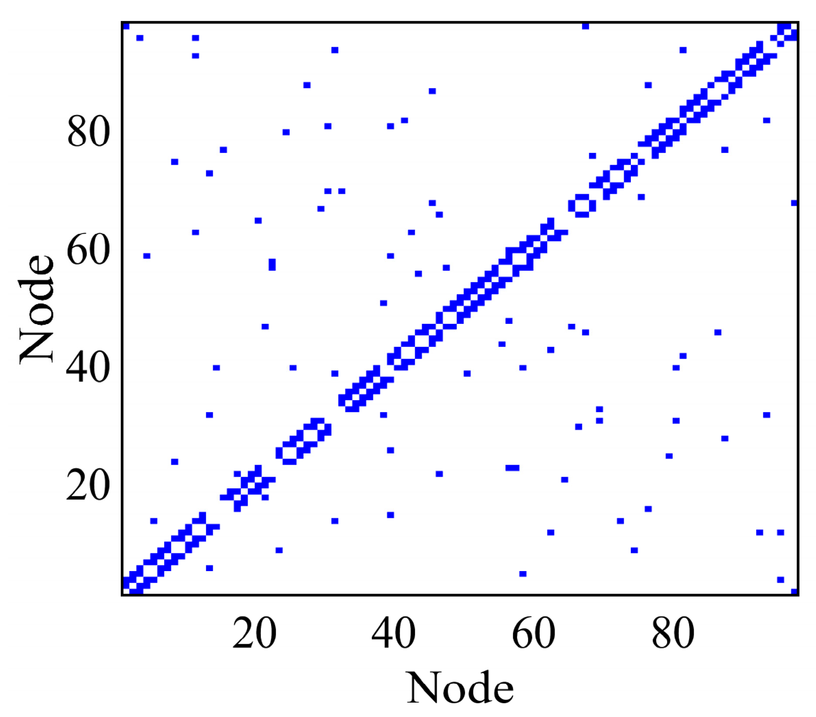
5.1. System Introduction

The developed example circuit comprises 190 components of resistors, capacitors, and inductors whose quantify ratio is set to 35:4:1. According to Section 2, the circuit can be abstracted as an impedance network whose topology with 98 nodes and 190 edges. The connection relationship of the network is shown in Figure 3. The impedance moduli of the components are assumed to be randomly generated between 10 and 1000, and the weights are set accordingly. The power supply voltage is set to 12 V and the frequency to 10 kHz. The initial currents of all components can be calculated by using the LTspice 17.1.15 software. The capacity parameter $\tau$ is set to be 1.

Temperature is the main factor that can cause component degradation, which is influenced by the component’s own heat, the ambient temperature, and the heat dissipation of the equipment. It is assumed that component temperature remains constant at 353 K during continuous operation. It is also assumed that degradation mainly occurs in two types of components: resistors and capacitors. The degradation rates for the same type of components are assumed to be equal. The degradation models can be presented in Equations (6) and (7), and the related parameters are listed in

Table 1. Degradation parameters of resistor and capacitor [3].

Component Type	Resistor				Capacitor
Parameter	EA,1/eV	$\beta$	${\alpha }_1$	${\sigma }_1$	EA,2/eV	${\alpha }_2$	${\sigma }_2$
Value	0.52	0.5	200	$2\times {10}^{-5}$	0.6	95.54	$1\times {10}^{-6}$

.

Considering the effect of random shocks, this case assumes that the shock frequency is $0.01h^{-1}$ and obeys a Poisson process. The shock stress acting on each component obeys a normal distribution $W_{k,ij}\sim N\left({\mu }_{ij},{\sigma }_{ij}^2\right)$, where the mean value ${\mu }_{ij}$ of the shock stress is $3I_{ij}\left(0\right)$ and the standard deviation ${\sigma }_{ij}$ is $0.1{\mu }_{ij}$. In addition, it is assumed that shock strength thresholds $W_{th,ij}={\mu }_{ij}+6{\sigma }_{ij}$, and shock trigger thresholds $W_{tr,ij}={\mu }_{ij}-3{\sigma }_{ij}$. Considering the effects of damage shocks on the impedance and the capacity thresholds, the impedance degradation coefficient $\zeta$ is set to be $5\times {10}^{-4}{Z}_{ij}/{\mu }_{ij}$, and the capacity degradation coefficient $\eta$ is set to be 0.0003. Based on the simulation algorithm presented in Section 4.3, the cascading failure propagation process of the current in this case is obtained using MATLAB 2019b software.

5.2. Cascading Failure Analysis

This section discusses the process of cascading failure propagation in the circuit when subjected to a combination of degradation and shock. The degradation and shock uncertainties are modeled by the Wiener process and Poisson process, respectively. The impedance network’s degradation trajectories obtained from each simulation differ as a result. Figure 4 displays several simulated degradation trajectories of the network at 353 K, where the blue and red lines represent the trajectories that consider both degradation and random shocks, while the green lines are the trajectories that only consider degradation for comparison purposes. In this case, the degradation trajectories considering degradation are simulated by the model given in ref. [3]. As can be seen in Figure 4a, the effect of random shocks causes the system to degrade or even collapse earlier than if only the degradation effect is considered. Under the present setup conditions, it is evident that shocks are primarily manifested in the form of damage shocks. These shocks mainly accelerate the occurrence of sudden changes in the network state. In addition, there are differences in the degradation trajectory when the effect of degradation and shock uncertainty is taken into account. Despite continuous degradation of internal components and exposure to random shocks, the system’s health state remains at a high level for an extended period [see Figure 4(b-1,c-1)]. This is mainly due to the fact that each component retains a relatively large margin to resist the increase in redistributed current. However, at a certain point, cascading failures propagate rapidly within the network, leading to the network reaching the failure threshold ($C{V}_{th}=0.5$) and eventual collapse [see Figure 4(b-2,c-2)]. Taking into account the combined effects of degradation and shock uncertainty, there is a dispersion of cascading failure paths and triggered failure times within the network. This results in differences in the variation curves of the network CV obtained from each simulation, as shown by the blue and red lines in Figure 4. Consequently, the failure times of different simulations will fall within a certain interval range and have statistical characteristics.

To investigate the impact of the component shock strength threshold $W_{th}$ on the cascading failure propagation of the impedance network, we further select two shock strength thresholds, 95% W_th,normal and 90% W_th,normal, under the same parameter settings. We perform the cascading failure propagation simulation, and the specific results are shown in Figure 5 and Figure 6, respectively. The figures demonstrate a notable difference in the degradation trajectories as the shock strength threshold decreases. Specifically, under the 95% W_th,normal condition, the impedance network’s health state CV follows a similar path to that under W_th,normal condition. However, when observing the CV change process in its early stages (refer to Figure 5b), it becomes apparent that the health state CV is no longer a curve that shows a smooth and slow decrease only affected by degradation. Instead, there are smaller abrupt changes. This is mainly due to the fact that, as the shock strength threshold $W_{th}$ decreases, random shocks may lead to the occurrence of hard failures and trigger the cascading failure propagation. However, during the initial stages of system operation, the impedance network’s higher capacity threshold enables it to suppress the propagation process more effectively. The time and extent of this mutation are also random due to the shock arrival time and the location of the component that triggers the hard failure. Compared to the normal shock strength threshold, the overall failure time of the network is more advanced, and the range of failure time distribution increases. The reason for this is that the shock stress is no longer limited to a single damage shock. A higher probability of fatal shock can directly lead to a component hard failure. Additionally, the reduction of the capacity threshold in the later stages of network operation inhibits the propagation of cascading failures, ultimately resulting in the direct collapse of the system.

However, if the shock strength threshold $W_{th}$ is reduced to 90%, the network’s health state degradation trajectory differs significantly from that observed at the W_th,normal and 95% W_th,normal settings. In this scenario, the impedance network undergoes stepwise degradation instead of a prolonged and gradual phase of degradation. By setting the failure threshold, the corresponding failure time is much smaller than that of the normal shock strength threshold. The probability of hard failure of components subjected to random shocks increases under the lower shock threshold setting. Furthermore, during the initial stage of system operation, the degradation effect of components is not significant for soft failures, resulting in more components being directly affected by hard failures. While the impedance network can prevent cascading failure in its initial stages, the failure of multiple components causes the remaining components to superimpose their redistributed currents. This ultimately results in the global propagation of the cascading failure within the system. As the shock strength threshold decreases, the main cause of the cascading failure shifts from degradation to shocks. Hard failures also replace soft failures as the main factor triggering the cascading failure.

To accurately describe the statistical characteristics of the failure time at various shock strength thresholds, we extract the failure time data from 1000 simulations. To determine the distribution form of the failure time data, the data are fitted with lognormal and Weibull distributions, respectively, estimated by the Maximum Likelihood Estimate (MLE) method and selected by the AIC criterion. Figure 7 displays the probability plots of the failure time data, and

Table 2. Parameter estimates for fitted distributions at different shock strength thresholds.

Wth	Distribution	Parameter Estimates 1	Parameter Estimates 2	Parameter Estimates 3	AIC
Wth,normal	Lognormal	$\widehat{\mu }=10.7986$	$\widehat{\sigma }=0.0673$	—	10588
	Weibull	$\widehat{\lambda }=58996$	$\widehat{k}=13.25$	—	10667
95% Wth,normal	Lognormal	$\widehat{\mu }=10.8607$	$\widehat{\sigma }=0.3132$	—	12011
	Lognormal (mixed)	$\widehat{\mu }=10.7849$	$\widehat{\sigma }=0.0811$	$p_1=0.0994$	10766
	Weibull (mixed)	$\widehat{\lambda }=39268$	$\widehat{k}=2.57$
	Weibull	$\widehat{\lambda }=57196$	$\widehat{k}=7.49$	—	11396
90% Wth,normal	Lognormal	$\widehat{\mu }=9.3942$	$\widehat{\sigma }=1.0058$	—	11687
	Weibull	$\widehat{\lambda }=17329$	$\widehat{k}=1.37$	—	11515

lists the parameter estimates and AIC for each distribution. It is evident that the failure time data conforms better to the lognormal distribution when the shock strength threshold is W_th,normal since it has the smallest AIC value, as shown in Figure 7a. Conversely, reducing the shock strength threshold to 90% W_th,normal results in the failure time data that more closely follows the Weibull distribution, as shown in Figure 7d. This also indirectly indicates that the cause of the system failure has fundamentally changed. However, when the shock strength threshold is 95% W_th,normal, neither of the two distribution types mentioned above (lognormal and Weibull) can fit all the failure time data better, as shown in Figure 7b,c. The degradation trajectories in this condition suggest that cascading failure is triggered by hard failure resulting from fatal shocks and soft failure resulting from a combination of degradation and damage shocks. The coexistence of these two types of failures is also reflected in the distribution characteristics of the failure time. Specifically, the failure data in the early stages of operation may be significantly related to hard failures. For failures that occur in the later stages of operation, degradation remains the primary cause. Therefore, fitting a single distribution may not accurately reflect the true failure behavior of the impedance network.

In order to better characterize the distribution of the failure time data at 95% W_th,normal, we fit the failure time data using a mixed distribution form of the Weibull distribution and the lognormal distribution, i.e.,

$$f\left(t\right)=p_1\cdot \frac{\beta }{\eta }{\left(\frac{t}{\eta }\right)}^{\beta -1}\exp \left[-{\left(\frac{t}{\eta }\right)}^{\beta }\right]+\left(1-p_1\right)\cdot \frac{1}{\sigma t\sqrt{2\pi }}\exp \left[-\frac{{\left(\ln t-\beta \right)}^2}{2{\sigma }^2}\right]$$

(23)

$$R\left(t\right)=p_1\cdot \exp \left[-{\left(\frac{t}{\eta }\right)}^{\beta }\right]+\left(1-p_1\right)\cdot \left[1-\mathsf{\Phi }\left(\frac{\ln t-\beta }{\sigma }\right)\right]$$

(24)

The parameters of this mixed distribution model are estimated by MLE. Figure 8 displays the probability plot of the failure time data, and Table 1 lists the parameter estimates for the mixed distribution. It is evident that the proposed distribution form effectively characterizes the failure of impedance networks at different stages of operation.

Based on the failure time data and the corresponding fitted distribution model, the network reliability curve can be obtained, as shown in Figure 9. In addition, we also extract and fit reliability curves considering only degradation under the same setup for comparison. It can be seen that the adopted distribution form and parameter estimates can better describe the variation of the network reliability, and the selection of the shock strength threshold has a significant effect on the reliability of the impedance network. Lowering the shock strength threshold significantly reduces the network’s reliability. The network can maintain a high level of reliability for a long period of operation when the shock strength threshold is W_th,normal. However, it decreases rapidly during the later operation period (40,000 h). According to the fitting results, the network’s reliable life at 90% of reliability is 44,796 h. If the shock strength threshold decreases to 95% W_th,normal, the lifetime may be affected. The network shows a gradual decline in reliability during the initial operation period, followed by a sharp decrease at 40,000 h. Although the impedance network can maintain a high level of reliability for an extended period, it experiences a rapid decline during the later stages of operation. However, it is important to note that the network is still guaranteed to operate normally for up to 40,000 h under these conditions. When the shock strength threshold drops to 90% W_th,normal, the network reliability significantly decreases during early operation. Its reliable life at 90% reliability can only be maintained for 3049 h.

6. Conclusions

This article proposed a component failure behavior model considering the degradation–shock correlation and analyzes the interactions between soft and hard failure processes among different components. Based on this, the cascading failure model with degradation and shock of a circuit system using an impedance network is constructed by combining current redistribution factors. A simulation algorithm is further proposed to simulate the cascading failure propagation behavior of the circuit system over its entire lifetime. The main conclusions are summarized below.

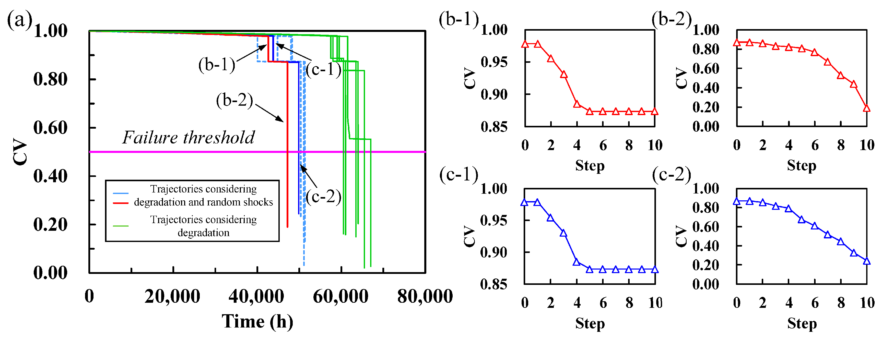
• Random shocks can affect the propagation behavior of cascading failure in a circuit system undergoing continuous degradation. When the shock strength threshold is high, external shocks mainly accelerate the evolution of cascading failure in the form of damage shocks. As the shock strength threshold decreases, the effects of shock become more pronounced. When the threshold drops to a certain level, the probability of hard failures due to random shocks increases. This makes the system capable of triggering cascading failures even in the early stages of operation. However, the circuit system’s capability to suppress cascading failures ensures that the system’s health state undergoes only minor abrupt changes. As the shock strength threshold decreases, more components experience hard failures, resulting in further superposition of redistributed currents in the remaining components. This causes the cascading failure to propagate globally. The main cause of cascading failure changes from continuous degradation dominance to random shock dominance, resulting in hard failure replacing soft failure as the main root cause of triggering cascading failure.
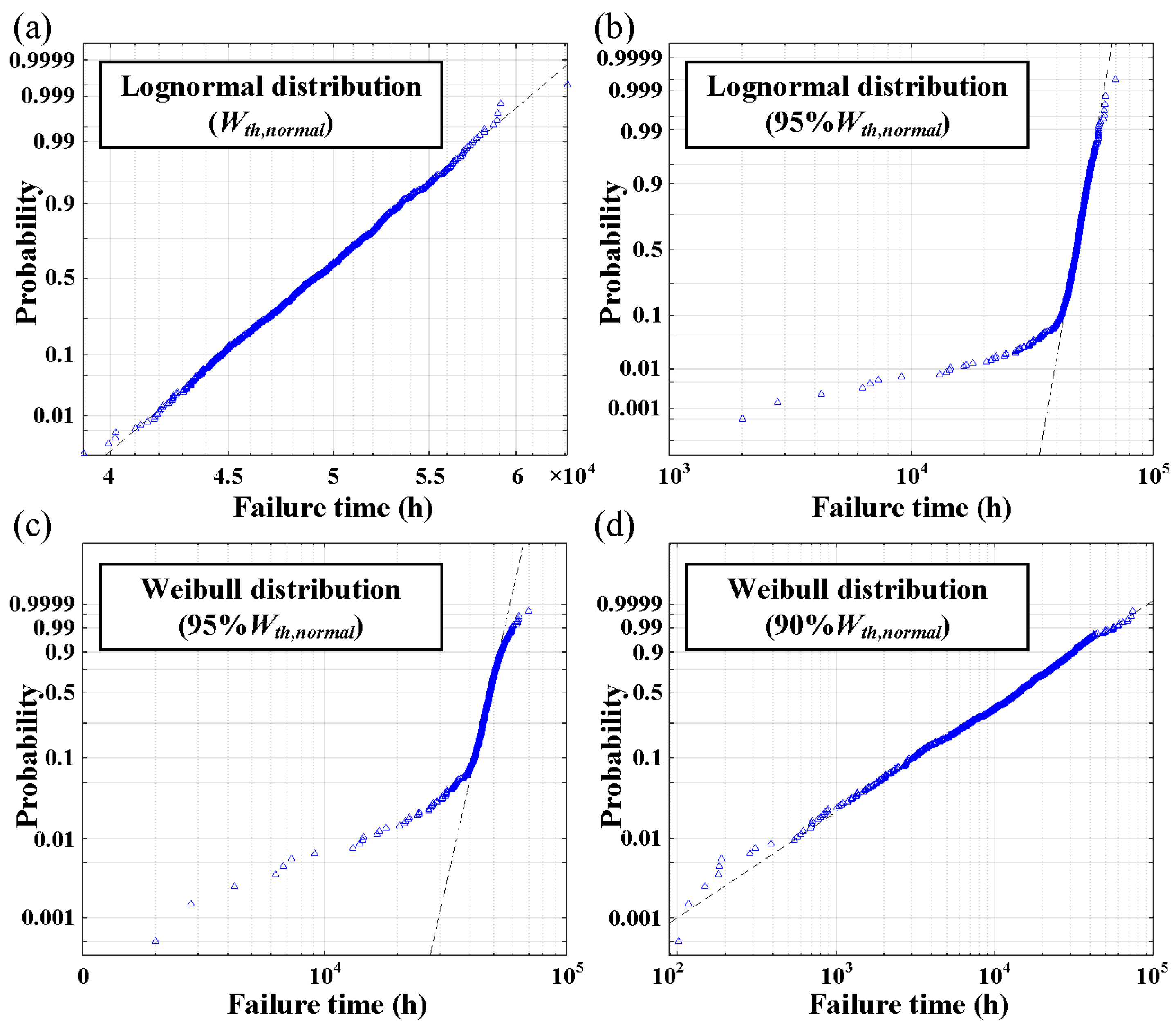
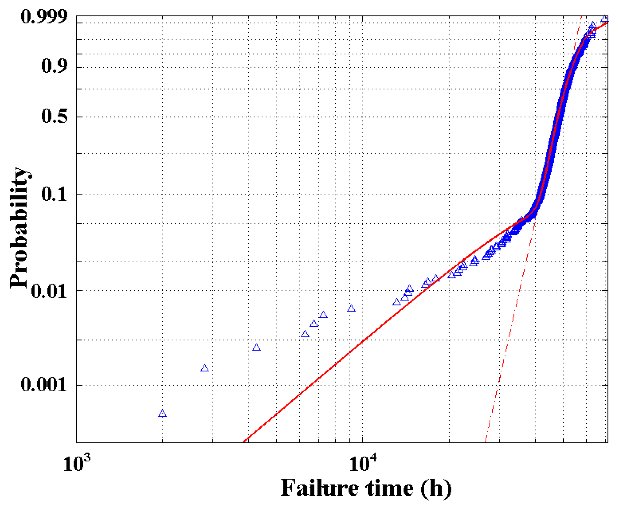
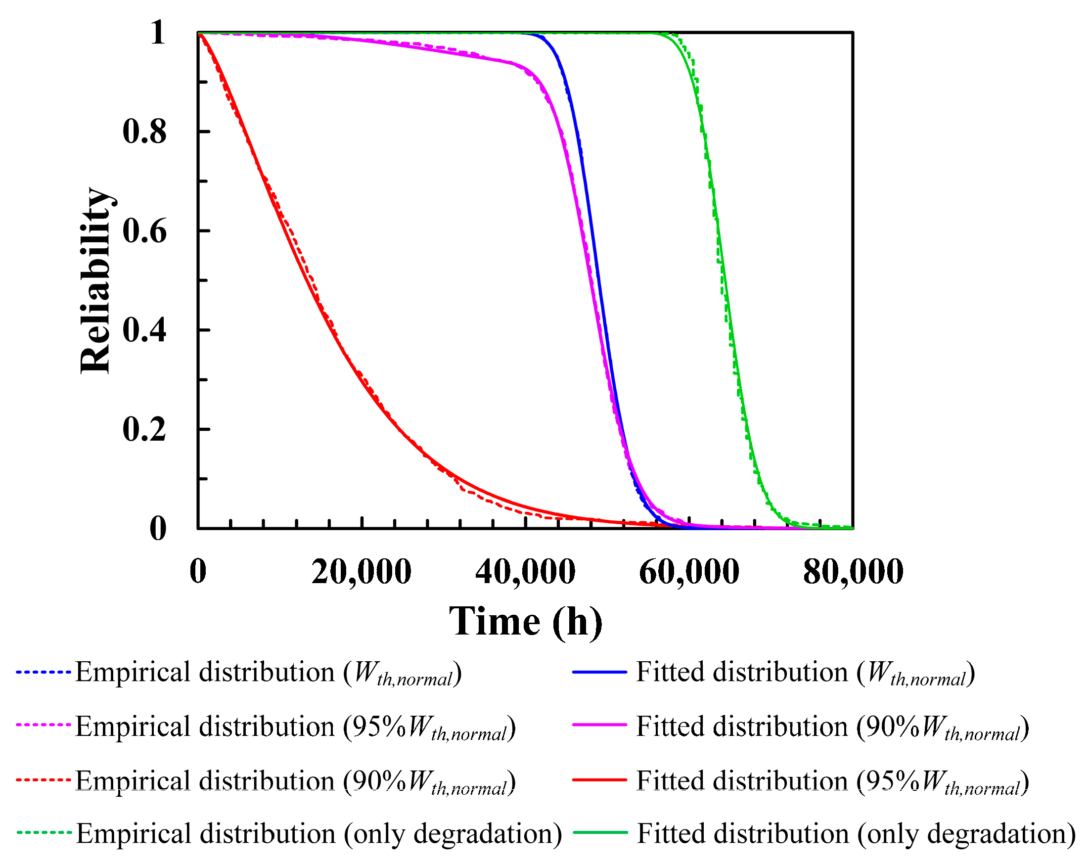
• At higher shock strength thresholds, the failure time of the circuit system follows the lognormal distribution, and the trigger cause of cascading failure is dominated by soft failures caused by degradation and damage shocks. However, at lower shock strength thresholds, the failure time conforms to the Weibull distribution, and the trigger cause of cascading failure is dominated by hard failures caused by fatal shocks. Within the range of the two types of threshold settings, there may be instances where soft and hard failures coexist. To evaluate the reliability of the circuit system under different operating periods, a mixed distribution model constructed using the Weibull and lognormal distributions can be effective compared to a single distribution.

References

1. Vasan, A.S.S.; Pecht, M.G. Electronic Circuit Health Estimation through Kernel Learning. IEEE Trans. Ind. Trial Electron. 2018, 65, 1585–1594. [Google Scholar] [CrossRef]
2. Jia, Z.; Liu, Z.; Gan, Y.; Vong, C.M.; Pecht, M. A Deep Forest-Based Fault Diagnosis Scheme for Electronics-Rich Analog Circuit Systems. IEEE Trans. Ind. Electron. 2021, 68, 10087–10096. [Google Scholar] [CrossRef]
3. Jin, Y.; Zhang, Q.; Chen, Y.; Lu, Z.; Zu, T. Cascading failures modeling of electronic circuits with degradation using impedance network. Reliab. Eng. Syst. Saf. 2023, 233, 109101. [Google Scholar] [CrossRef]
4. Jin, Y.; Chen, Y.; Lu, Z.; Zhang, Q.; Kang, R. Cascading Failure Modeling for Circuit Systems Using Impedance Networks: A Current-Flow Redistribution Approach. IEEE Trans. Ind. Electron. 2021, 68, 632–641. [Google Scholar] [CrossRef]
5. Shi, J.; He, Q.; Wang, Z. GMM Clustering-Based Decision Trees Considering Fault Rate and Cluster Validity for Analog Circuit Fault Diagnosis. IEEE Access 2019, 7, 140637–140650. [Google Scholar] [CrossRef]
6. Sharifi, M.; Taghipour, S. Optimizing a redundancy allocation problem with open-circuit and short-circuit failure modes at the component and subsystem levels. Eng. Optim. 2021, 53, 1064–1080. [Google Scholar] [CrossRef]
7. Leroux, H.; Andreu, D.; Godary-Dejean, K. Handling Exceptions in Petri Net-Based Digital Architecture: From Formalism to Implementation on FPGAs. IEEE Trans. Ind. Inform. 2015, 11, 897–906. [Google Scholar] [CrossRef]
8. Zhai, G.; Zhou, Y.; Ye, X. A Tolerance Design Method for Electronic Circuits Based on Performance Degradation. Qual. Reliab. Eng. Int. 2015, 31, 635–643. [Google Scholar] [CrossRef]
9. Nakao, H.; Yonezawa, Y.; Sugawara, T.; Nakashima, Y.; Kurokawa, F. Online Evaluation Method of Electrolytic Capacitor Degradation for Digitally Controlled SMPS Failure Prediction. IEEE Trans. Power Electron. 2018, 33, 2552–2558. [Google Scholar] [CrossRef]
10. Li, D.; Zhang, Q.; Zio, E.; Havlin, S.; Kang, R. Network reliability analysis based on percolation theory. Reliab. Eng. Syst. Saf. 2015, 142, 556–562. [Google Scholar] [CrossRef]
11. Wu, C.W. Evolution and Dynamics of Complex Networks of Coupled Systems. IEEE Circuits Syst. Mag. 2010, 10, 55–63. [Google Scholar] [CrossRef]
12. Wang, W.X.; Chen, G. Universal robustness characteristic of weighted networks against cascading failure. Phys. Rev. E 2008, 77, 026101. [Google Scholar] [CrossRef]
13. Fan, Y.; Cheng, Y.; Chen, Y.; Yang, Y. Analysis of cascading failure of circuit systems based on load-capacity model of complex network. In Proceedings of the 2nd International Conference on Reliability Systems Engineering (ICRSE 2017), Beijing, China, 10–12 July 2017; p. R089. [Google Scholar]
14. Rommes, J.; Schilders, W.H.A. Efficient Methods for Large Resistor Networks. IEEE Trans. Comput. Aided Des. Integr. Circuits Syst. 2010, 29, 28–39. [Google Scholar] [CrossRef]
15. Mei, S.; Raghavan, N.; Bosman, M.; Pey, K.L. Stochastic Modeling of FinFET Degradation Based on a Resistor Network Embedded Metropolis Monte Carlo Method. IEEE Trans. Electron Devices 2018, 65, 440–447. [Google Scholar] [CrossRef]
16. Van Mieghem, P.; Devriendt, K.; Cetinay, H. Pseudoinverse of the Laplacian and best spreader node in a network. Phys. Rev. E 2017, 96, 032311. [Google Scholar] [CrossRef] [PubMed]
17. Lehmann, J.; Bernasconi, J. Current redistribution in resistor networks: Fat-tail statistics in regular and small-world networks. Phys. Rev. E 2017, 95, 032310. [Google Scholar] [CrossRef] [PubMed]
18. Lehmann, J.; Bernasconi, J. Stochastic load-redistribution model for cascading failure propagation. Phys. Rev. E 2010, 81, 031129. [Google Scholar] [CrossRef] [PubMed]
19. Hou, Y.; Xing, X.; Li, M.; Zeng, A.; Wang, Y. Overload cascading failure on complex networks with heterogeneous load redistribution. Phys. A-Stat. Mech. Its Appl. 2017, 481, 160–166. [Google Scholar] [CrossRef]
20. Kang, F.; Cui, L.; Ye, Z.; Zhou, Y. Reliability analysis for systems with self-healing mechanism in degradation-shock dependence processes with changing degradation rate. Reliab. Eng. Syst. Saf. 2024, 241, 109671. [Google Scholar] [CrossRef]
21. Cao, S.; Wang, Z.; Liu, C.; Wu, Q.; Li, J.; Ouyang, X. A novel solution for comprehensive competing failure process considering two-phase degradation and non-Poisson shock. Reliab. Eng. Syst. Saf. 2023, 239, 109534. [Google Scholar] [CrossRef]
22. Wu, B.; Zhang, Y.; Zhao, S. Modeling coupled effects of dynamic environments and zoned shocks on systems under dependent failure processes. Reliab. Eng. Syst. Saf. 2023, 231, 108911. [Google Scholar] [CrossRef]
23. Hu, J.; Sun, Q.; Ye, Z.S. Condition-Based Maintenance Planning for Systems Subject to Dependent Soft and Hard Failures. IEEE Trans. Reliab. 2021, 70, 1468–1480. [Google Scholar] [CrossRef]
24. Zeng, Z.; Barros, A.; Coit, D. Dependent failure behavior modeling for risk and reliability: A systematic and critical literature review. Reliab. Eng. Syst. Saf. 2023, 239, 109515. [Google Scholar] [CrossRef]
25. Bian, L.; Wang, G.; Liu, P. Reliability analysis for k-out-of-n(G) systems subject to dependent competing failure processes. Comput. Ind. Eng. 2023, 177, 109084. [Google Scholar] [CrossRef]
26. Song, S.; Coit, D.W.; Feng, Q.; Peng, H. Reliability Analysis for Multi-Component Systems Subject to Multiple Dependent Competing Failure Processes. IEEE Trans. Reliab. 2014, 63, 331–345. [Google Scholar] [CrossRef]
27. Shen, J.; Elwany, A.; Cui, L. Reliability analysis for multi-component systems with degradation interaction and categorized shocks. Appl. Math. Model. 2018, 56, 487–500. [Google Scholar] [CrossRef]
28. Schaub, M.T.; Lehmann, J.; Yaliraki, S.N.; Barahona, M. Structure of complex networks: Quantifying edge-to-edge relations by failure-induced flow redistribution. Netw. Sci. 2014, 2, 66–89. [Google Scholar] [CrossRef]
Figure 1. Two types of failure processes of the component ij. (a-1) damage shocks and safety shocks during random shocks. (a-2) Hard failure process caused by fatal shocks; (b-1) impedance change process caused by degradation and damage shocks; (b-2) impedance change process caused by degradation and damage shocks when the fatal shock is not reached; (c-1) soft failure process caused by the current and capacity threshold changes due to the influence of impedance changes; (c-2) the processes of change in the current and capacity threshold when the fatal shock is not reached.
Symmetry 16 00488 g001
Figure 2. Simulation framework for cascading failure propagation process with degradation and shock.
Symmetry 16 00488 g002
Figure 3. Connection relationship of the impedance network.
Symmetry 16 00488 g003
Figure 4. (a) Degradation trajectory of the impedance network at 353 K. (b-1) the degradation process due to fast dynamic propagation at 42,644 h in the first simulation; (b-2) the collapse process due to fast dynamic propagation at 47,179 h in the first simulation; (c-1) the degradation process due to fast dynamic propagation at 43,812 h in the second simulation; (c-2) the collapse process due to fast dynamic propagation at 49,858 h in the second simulation.
Symmetry 16 00488 g004
Figure 5. Degradation trajectory of the impedance network with shock strength threshold of 95% Wth,normal at 353 K, different colors of lines indicate the results of six different simulations affected by the randomness of degradation and shocks. (a) the entire process of impedance network failure; (b) the degradation process of impedance network in the early stages, which is able to resist the cascading failure propagation.
Symmetry 16 00488 g005
Figure 6. Degradation trajectory of the impedance network with shock strength threshold of 90% Wth,normal at 353 K, different colors of lines indicate the results of six different simulations affected by the randomness of degradation and shocks.
Symmetry 16 00488 g006
Figure 7. Failure time data probability plot at different shock strength thresholds. (a) lognormal distribution (Wth,normal); (b) lognormal distribution (95%Wth,normal); (c) Weibull distribution (95%Wth,normal); (d) Weibull distribution (90%Wth,normal).
Symmetry 16 00488 g007
Figure 8. Failure time data probability plot for mixed distribution at 95% Wth,normal.
Symmetry 16 00488 g008
Figure 9. Empirical and fitted distribution of reliability at different shock strength thresholds.
Symmetry 16 00488 g009