Controlled State Transfer in Central Spin Models

Abstract

In the recent literature, various aspects of the transfer of quantum states by spin chains have been thoroughly investigated. Part of the existing study is devoted to the problem of optimal control, with the goal of achieving a highly reliable information/state transfer for a given time T. In general, achieving this goal is not an easy task in the case of (open) quantum systems. Various approaches have been developed and applied, including Krotov’s method to study the problem. It is a gradient-based method used here to study the problem of state transfer control in central spin models. Our results show that with Krotov’s method, it is possible to find an optimal control form that allows for very-high-fidelity state transfer in the central spin models we have developed. Our results will be of interest for a better understanding of the non-trivial effects of the classical world on the quantum world, which have been discussed in the form of various new effects, including the Epstein effect, in the recent literature.

1. Introduction

In recent years, the scientific community has made significant advances in computational and experimental science that have dramatically changed our understanding of the quantum world and its interaction with the classical world. The evolution of a quantum system is directly related to the influence of the environment. The coupling with the reservoir, which can be either a bath or an environment, plays a significant role in the properties of a quantum system, which significantly influences quantum technology and its progress. The (optimal) control of quantum systems is an important research topic as it is applied in the development of new technologies. One of the directions in modern science in which it plays a crucial role is quantum information processing tasks, where quantum information must be sent through a quantum network. It is obvious that the goal is to develop complex systems capable of processing and solving complex information and problems. It is already known that spin chain systems have great potential for practical application in quantum technology, including quantum information, quantum communication and quantum computation [1,2,3,4,5,6,7,8,9,10,11,12,13,14,15,16,17,18,19,20,21,22,23,24] (and references therein), to name but a few.

In this paper, we have taken a step towards understanding state transfer in central spin models by treating it as an optimal control problem. Our goal is to obtain the optimal control for the systems considered in this work at a particular time T. The analysis performed has shown that the gradient-based Krotov’s method is a robust approach to achieve the goal for central spin models and can solve the problem very efficiently. Furthermore, by utilizing this method, we have established a specific type of coupling between the last spin and the bath of the central spin models. This has greatly enhanced the robustness of the control, allowing for high-fidelity state transfer to be achieved. Our interest in studying central spin models is related to their specific structure (a single spin-half particle interacting with a spin environment/spin bath) and the fact that they can be used to describe various processes, e.g., the decoherence of the system over time. On the other hand, various studies have shown that the central spin extends the available degrees of freedom and makes the bath a useful resource. In these models, the central spin typically interacts with the bath spins through anisotropic Heisenberg interactions. The fully isotropic $XXX$ model is generally accepted to model systems with spherical symmetry, and the quantum dot is one of these models (see for example [25,26,27,28,29,30,31,32,33,34,35,36,37,38,39,40,41] and the references therein for further discussion of central spin models and their applications). Given the above discussion, state transfer in central spin models was one of the first problems to be studied and understood. In this paper, we will consider state transfer in two models, Type I and Type II. The difference between the models lies in the form of the interaction between the central spin particle and the bath particles, which we have taken into account. In the case of the Type I model, which is based on the standard central spin model, a high-fidelity state transfer for a predetermined time T has been achieved due to the symmetry used to develop the interaction between the last spin and the bath of the central spin model. On the contrary, the Type II model is a new model where next-nearest-neighbour interactions between the bath spins have been introduced. By developing an interaction between the last spin in the chain and the bath based on the idea of next-nearest-neighbour interactions, we have again achieved a high-fidelity state transfer for a predetermined time T. It is important to stress that the developed interactions between the spins in both models have turned the control of the bath into a source to achieve high fidelity and robust state transfer. This highlights the importance of the bath in achieving these results. In conclusion, we want to emphasize that by examining three scenarios, we were able to determine which components of the models require control to achieve high-fidelity state transfer. One of our findings clearly showed that controlling the final spin for the state transfer may not be the most optimal decision. This also implies that systems such as these can offer a high degree of information transfer protection if the other parts of the system are adequately safeguarded. Our results are of great interest for a better understanding of a non-trivial influence of the classical world on the quantum world, as it is the case of the Epstein effect. It seems that vibrations modulated from the classical world affect the quantum world, playing a central role in the Epstein effect. Broadly defined, the Epstein effect consists of modulating the effect of vibration from one fluid to other fluid regions or distinct fluids. Moreover, experimental studies revealing the Epstein effect indicate, for instance, that information from the initial high-density regime can be transferred to the low-density regime without significant changes [42] (see also [43]).

The present work is structured as follows: Section 2 discusses the mathematical formalism used to model the quantum systems under consideration, allowing us to follow the results obtained. On the other hand, in Section 3, we will describe the central spin models that we have been developed. In Section 4 and Section 5, we present and discuss in detail the results of our study based on numerical simulations. Section 6 then presents the conclusion from our analysis.

2. Optimal Control and Krotov’s Method

Closed quantum systems are only an idealization of the real world, and in almost all cases, it is not possible to avoid/neglect the external effects. On the other hand, the whole system can be divided on the basis of certain assumptions and represented as a system of interest and the environment. However, the representation should be a reasonable one that allows the full dynamics of the system to be solved. Considering the nature of the problem in this paper, we assume that the above problem can be solved efficiently, and the Hamiltonian of our systems can be represented in the following way,

$$H\left(t\right)=H_0+\sum _l{ϵ}_l\left(t\right)H_l,$$

(1)

which allows us to represent the main problem as a control problem, where $H_0$ is the time-independent uncontrolled part of the Hamiltonian, $H_l$ is the time-independent Hamiltonian describing the control strategy, and ${ϵ}_l\left(t\right)$ is the corresponding time-dependent control function. In the following, we present only the most important aspects of the applied approach to perform the simulations and follow the discussion in Section 4 and Section 5, respectively. In particular, we will discuss the Krotov’s method, which requires a trial solution of the control function $ϵ\left(t\right)$. This reduces the task to an iterative optimization of the shape of the control function by minimizing a function J

$$J\left[s,{ϵ}_l^{\left(i\right)}\left(t\right)\right]=J_T\left(s\right)+\sum _l{\int }_0^{T}g\left({ϵ}_l^{\left(i\right)}\left(t\right)\right),$$

(2)

where $s={\varphi }_i\left(t\right)$ is the set of wave functions at the i-th iteration, while ${ϵ}_l^{\left(i\right)}\left(t\right)$ is the set of control functions. In the above equation, the function g tracks the running costs of the control fields and has the following form:

$$g=\frac{{\lambda }_{a,l}}{S_l\left(t\right)}{\left(\Delta {ϵ}_l^{\left(i\right)}\left(t\right)\right)}^2.$$

(3)

Here, ${\lambda }_{a,l}$ is an inverse step size, $S_l\left(t\right)\in [0,1]$ is an update shape function, while the difference of the control function between the current and the last iteration is given by $\Delta {ϵ}_l^{\left(i\right)}\left(t\right)$

$$\Delta {ϵ}_l^{\left(i\right)}\left(t\right)=\frac{S_l\left(t\right)}{{\lambda }_{a,l}}Im\left(\langle {\xi }^{(i-1)}\left(t\right)|\frac{\partial H^{\left(i\right)}\left(t\right)}{\partial {ϵ}_l^{\left(i\right)}\left(t\right)}|{\varphi }^{\left(i\right)}\left(t\right)\rangle \right),$$

(4)

with $|{\xi }^{(i-1)}\left(t\right)\rangle$ to be back-propagated using the Hamiltonian under the previous iteration’s control fields with the following boundary condition $|{\xi }^{(i-1)}\left(T\right)\propto {\varphi }_f\rangle$, while $H^{\left(i\right)}\left(t\right)$ is the total Hamiltonian of the i-th iteration. On the other hand, we consider $J_T$ in Equation (2) as the infidelity of the evolved state or the target state,

$$J_T\left(s\right)=1-|\langle {\varphi }_f|{\varphi }^i\left(T\right)\rangle {|}^2,$$

(5)

with $|{\varphi }_f\rangle$ as the target state.

To conclude this section, we would like to remind the reader that the state of an open quantum system is a mixed state represented by a density matrix (density operator)

$$\rho =\sum _i{p}_i|{\varphi }_i\rangle \langle {\varphi }_i|,$$

(6)

where $|{\varphi }_i\rangle$ is the pure state in the ensemble, while $p_i$ is the corresponding probability of occurrence. The time evolution of a mixed state can be calculated simply by combining Equation (6) and the time-dependent Schrodinger equation

$$i\hslash \frac{d}{dt}|\varphi \left(t\right)\rangle =\widehat{H}|\varphi \left(t\right)\rangle ,$$

(7)

giving us the well-known Lindblad master equation (Markovian approximation)

$$\frac{d\rho }{dt}=\mathcal{L}\rho =-i[\widehat{H},\rho ]+\sum _i{\gamma }_i\left(c_i\rho c_i^{+}-\frac{1}{2}{c}_i^{+}{c}_i\rho -\frac{1}{2}\rho c_i^{+}{c}_i\right),$$

(8)

where $\widehat{H}$ is the Hamiltonian of the system under consideration, while ${\gamma }_i$ and $c_i$ are the dissipation rate and the jump operator, respectively. In the above equation, $[\widehat{H},\rho ]=\widehat{H}\rho -\rho \widehat{H}$. Finally, we must remember that the fidelity should be calculated according to the following equation:

$$F({\rho }_1,{\rho }_2)={\left[Tr{\left(\sqrt{{\rho }_1}{\rho }_2\sqrt{{\rho }_1}\right)}^{1/2}\right]}^2,$$

(9)

where ${\rho }_1$ is the density matrix of the state to be transferred, while ${\rho }_2$ is the density matrix of the final state. Our results, which we discuss in Section 4 and Section 5, are based on the Python implementation of Krotov’s method [44], which is based on QuTiP [45,46]. We recommend the reader to refer to the excellent tutorial of both tools for more information about the methods, how they have been implemented, how they are connected to each other, and to gain practical experience by following the provided examples therein.

3. Models

The Type I model that we study here is a hybrid model described by the following Hamiltonian ($\hslash =1$)

$${\widehat{H}}^I={\widehat{H}}_{cs}^I+{\widehat{H}}_{tail}^I,$$

(10)

with the central spin system ($1/2$ spin central particle)

$${\widehat{H}}_{cs}^I={\omega }_0{S}_0^z+\sum _i^{L-1}{\omega }_i{S}_i^z+{\widehat{H}}_{cs-bath}^I,$$

(11)

and

$${\widehat{H}}_{cs-bath}^I=\sum _i^{L-1}{g}_i\left(S_0^x{S}_i^x+S_0^y{S}_i^y+\alpha S_0^z{S}_i^z\right),$$

(12)

representing the interaction between the central spin particle and the bath. In the above equations, $\{S^x,S^y,S^z\}$ are Pauli matrices, $g_i$ is the (in)homogeneous strength of the interaction between the central qubit and the i-th bath spin, ${\omega }_0$ is considered as a local external field on the central qubit, while ${\omega }_i$ is a field on the bath spins. In general, the qubit–bath interaction is not isotropic and the parameter $\alpha$ in Equation (11) determines the anisotropy ($XXZ$ model). Moreover, ${\omega }_0$, ${\omega }_i$ and $g_i$ can be a function of time. On the other hand, we have assumed that ${\widehat{H}}_{tail}^I$ in Equation (10),

$${\widehat{H}}_{tail}^I\propto S_{L-1}^x{S}_L^x+S_{L-1}^y{S}_L^y+\alpha S_{L-1}^z{S}_L^z,$$

(13)

represents an interaction between the last spin of the bath of the central spin model with the $1/2$ spin particle, to which the state of the first (central) spin of the chain under consideration must be transferred.

The Type II model that we are studying is also a hybrid model described by the following Hamiltonian,

$${\widehat{H}}^{II}={\widehat{H}}_{cs}^{II}+{\widehat{H}}_{tail}^{II},$$

(14)

but here, we have modified the bath part as follows (next-nearest-neighbour interactions)

$${\widehat{H}}_{cs-bath}^{II}=\sum _i^{L-1}{g}_i\left(S_0^x{S}_i^x{S}_{i+1}^x+S_0^y{S}_i^y{S}_{i+1}^y+\alpha S_0^z{S}_i^z{S}_{i+1}^z\right),$$

(15)

with

$${\widehat{H}}_{cs}^{II}={\omega }_0{S}_0^z+\sum _i^{L-1}{\omega }_i{S}_i^z+{\widehat{H}}_{cs-bath}^{II}.$$

(16)

In addition, the interaction between the bath of the considered central spin model and the $1/2$ spin particle, to which the state of the first (central) spin of the considered chain must be transferred, was assumed as follows:

$${\widehat{H}}_{tail}^{II}\propto S_{L-2}^x{S}_{L-1}^x{S}_L^x+S_{L-2}^y{S}_{L-1}^y{S}_L^y+\alpha S_{L-2}^z{S}_{L-1}^z{S}_L^z.$$

(17)

In the above equations, L represents the total number of spins used to create the model. In the next two sections, we will discuss how to reduce the state transfer problem for the considered spin models to an optimal control problem and treat it with Krotov’s method. Given the many possibilities that can be realized with numerical analysis, we must limit ourselves to the most interesting results. In our analysis, we used the Python implementation of Krotov’s method built on QuTiP, which allowed us to reduce the complexity of the analysis. In our opinion, the structure of the previous two sections is relatively simple to follow, and interested readers can reproduce our results with some effort by uncovering other aspects of the models that were not covered in this study.

4. State Transfer in Model Type I

In this particular study, we are interested in the optimal control of an external drive pulse that allows us to achieve a very high fidelity state transfer. At this moment, we are not so much interested in modeling the source that generates the pulse. Instead, we treat the pulse as an influence of the classical world on the quantum world. After the presented clarification, we must first formulate the problem of state transfer as an optimal control problem that allows us to apply Krotov’s method. To achieve this goal, in a first step, we have rewritten the model given by Equations (10)–(13) in the following way:

$$H_0=\sum _i^{L-1}{\omega }_i{S}_i^z+\sum _i^{L-1}{g}_i\left(S_0^x{S}_i^x+S_0^y{S}_i^y+\alpha S_0^z{S}_i^z\right)+g_L\left(S_{L-1}^x{S}_L^x+S_{L-1}^y{S}_L^y+\alpha S_{L-1}^z{S}_L^z\right),$$

(18)

and

$$H_l=ϵ\left(t\right)S_0^z,$$

(19)

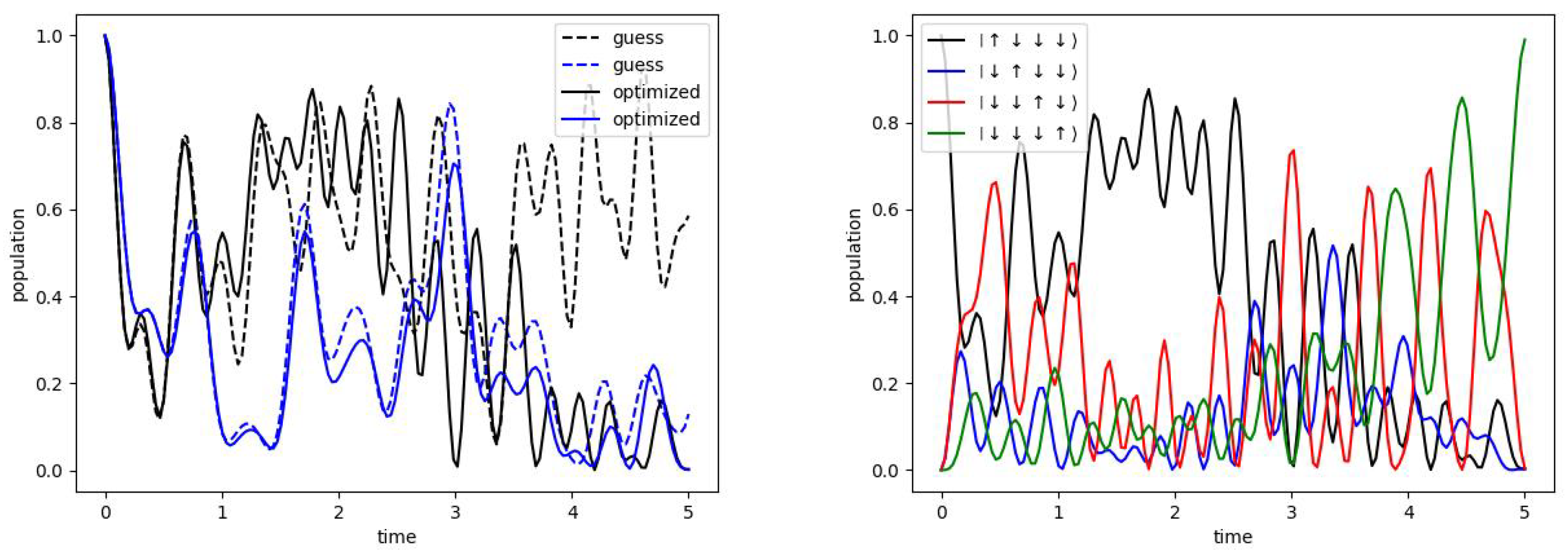
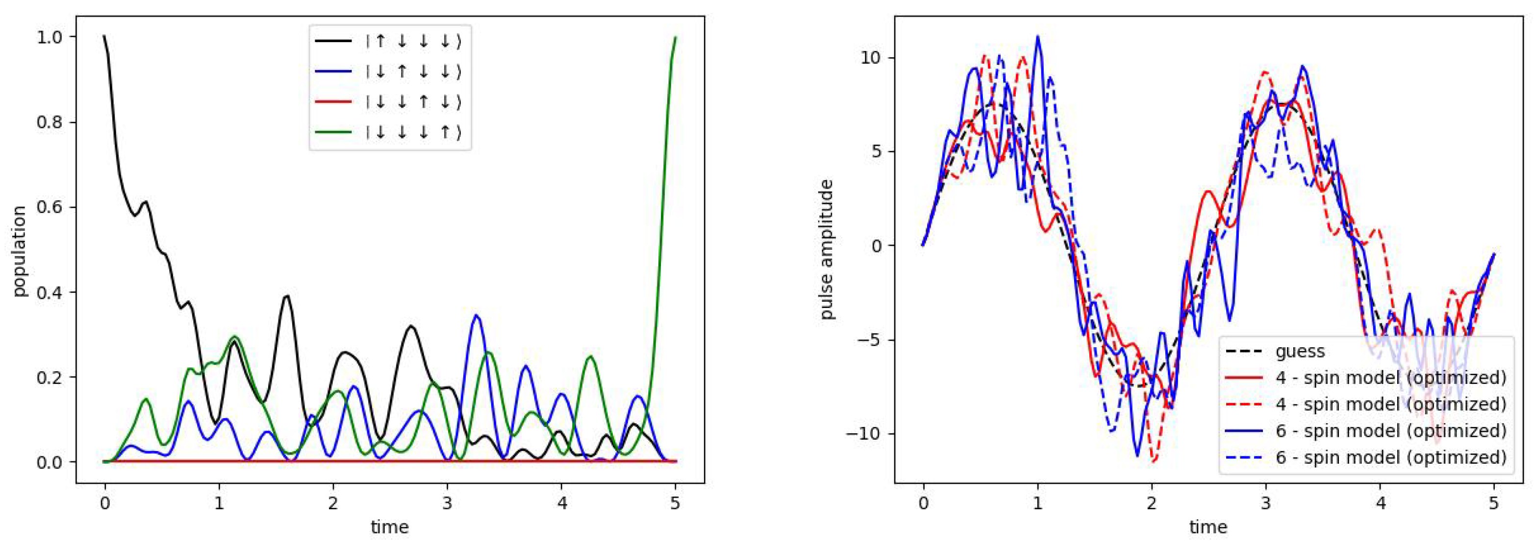
which indicate the time-independent uncontrolled and the time-independent controlled strategies of the model. The particular case presented above is an optimal control problem, where the goal is to find the form of the $ϵ\left(t\right)$ pulse applied to the first (central) spin in order to transfer its state to the final spin of the chain. Using numerical tools, we were able to study the state transfer problem for a variety of model parameters and concluded that Krotov’s method is indeed a very robust method. One of the results of our analysis can be seen in Figure 1. The plot on the left side of Figure 1 represents the population dynamics for the assumed and optimized signals, respectively. The black dashed (guessed pulse) and solid curves (optimized pulse) represent the case in which the model evolves from the initial $\left|\uparrow \downarrow \downarrow \downarrow \right.〉$ state to the $\left|\downarrow \downarrow \downarrow \uparrow \right.〉$ state. On the other hand, the blue curves similarly represent the case where the initial state of the system was $\left|\uparrow \uparrow \uparrow \downarrow \right.〉$, while the final state was assumed to be $\left|\downarrow \uparrow \uparrow \uparrow \right.〉$. We can clearly see that with Krotov’s method, the shape of the pulse was indeed optimized, and the goal was achieved. In addition, the fidelity in this case was estimated to be $F\approx 0.98$.

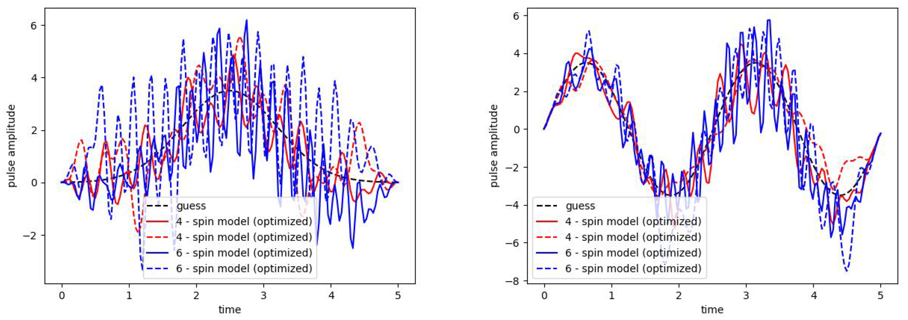
The plot on the right-hand side of Figure 1 shows the population dynamics for the optimized pulse. In both cases, $ϵ\left(t\right)\propto sin\left({\omega }_{d}t\right)$ and $L=4$ (the values of the parameters can be found in the caption of Figure 1). The results shown in Figure 2 show the guessed and optimized shapes of two pulses for 4 and 6 spin models, respectively. Having in mind the practical applications of the state transfer problem, we have analyzed the case where the controlling Hamiltonian is the bath part of the model given by Equation (12). Furthermore, in this case, we were able to obtain a very accurate state transfer ($F\approx 0.98$) using Krotov’s method, even for the cases where T is much smaller than T that we have shown in the plots.

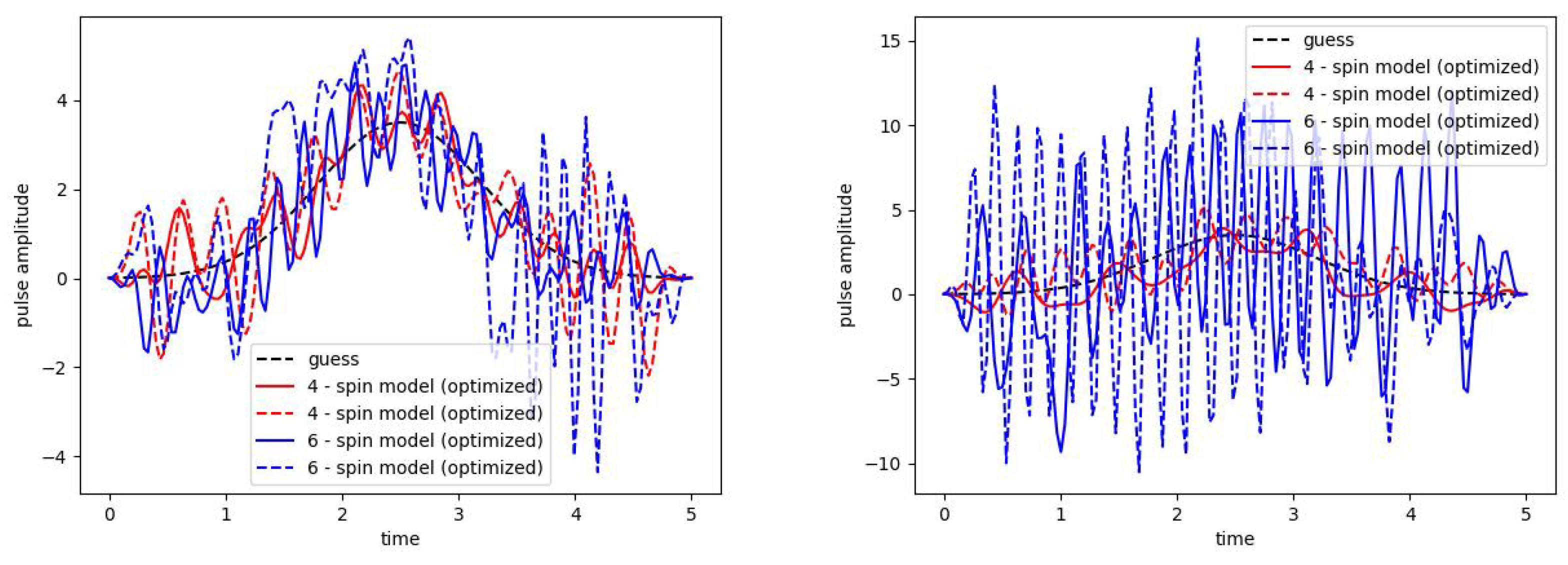
One of the results corresponding to this case can be found in Figure 3 when the initial pulse shape is a Gaussian. On the other hand, the analysis of the cases in which the external pulse is applied to the last spin of the chain to which the initial spin state should be transferred revealed interesting deviations from the previous two cases. In particular, we found that it is still possible to optimize the pulse shape to achieve a very-high-fidelity state transfer, as in the case of the two previous scenarios. However, in this scenario, more time is usually needed to achieve the goal. Actually, this is an expected result with a positive consequence that points to opportunities for developing algorithms to protect spin-chain networks from external attacks. The plot on the right side of Figure 3 shows one of the results for this case. To conclude this section, we can emphasize that the transfer of states using a central spin model is possible with high accuracy and that Krotov’s method can be applied to achieve the goal. The different possibilities that can be analyzed numerically provide a great opportunity to develop more complex systems to transfer even more complex states, which will be discussed in the upcoming papers. Some of the possibilities and tasks are discussed in the last section of this paper and indicate the direction in which our recent study can be extended.

5. State Transfer in Model Type II

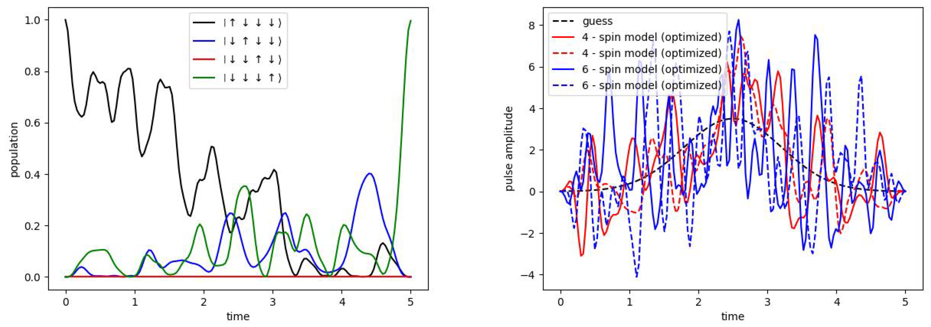
The analysis of model Type II has also shown that the state transfer by the modified central spin model given by Equations (14)–(17) can be achieved with $F\approx 0.98$. In Figure 4, we can find the population transfer for the model given by

$${\widehat{H}}_{cs-bath}^{II}=g_1\left(S_0^x{S}_1^x{S}_2^x+S_0^y{S}_1^y{S}_2^y+\alpha S_0^z{S}_1^z{S}_2^z\right)+$$

$$g_2\left(S_0^x{S}_2^x{S}_3^x+S_0^y{S}_2^y{S}_3^y+\alpha S_0^z{S}_2^z{S}_3^z\right),$$

(20)

and

$${\widehat{H}}_{tail}^{II}=g_3\left(S_2^x{S}_3^x{S}_4^x+S_2^y{S}_3^y{S}_4^y+\alpha S_2^z{S}_3^z{S}_4^z\right).$$

(21)

In this particular case, the model evolves from the initial $\left|\uparrow \downarrow \downarrow \downarrow \right.〉$ state to the $\left|\downarrow \downarrow \downarrow \uparrow \right.〉$ state. A Gaussian pulse was assumed as the initial pulse, which is applied to the first spin in the chain whose state is to be transferred. The results in terms of population transfer, shown on the left side of Figure 4, and the optimized shapes of the guess pulse, shown on the right side of the same figure, clearly show that Krotov’s method provides a solution. Moreover, the optimized shape of the guess pulse in the case of the model with $L=6$ can also be found on the right side of Figure 4. The results corresponding to the guess pulse $ϵ\left(t\right)\propto sin\left({\omega }_{d}t\right)$ can be seen in Figure 5. It should be emphasized that the external pulse applied to the bath part of the model allowed us to obtain a very-high-fidelity state transfer even for relatively small times T, which we used in the discussed results. However, we found that more time than the considered time T is required to achieve reliable state transfer when the pulse was applied to the last spin to drive state transfer in the considered model. Since the qualitative results are the same for both models to save space, we have not presented them explicitly here.

6. Conclusions

Achieving high-fidelity state transfer is one of the most important problems that must be solved in order to develop high-quality complex quantum systems used, for example, in quantum technology. Therefore, understanding how this can be realized theoretically and experimentally and how it can be controlled has already attracted much attention in the recent literature. On the other hand, the study of various complex systems would not be possible at all without numerical simulations. Spin-chain systems hold great potential for practical applications in quantum technology in the broadest sense. Therefore, enormous efforts have been made in recent years to understand the mechanism that enables reliable state transfer in different spin models. In this work, we have taken a step towards understanding the problem of state transfer in central spin models, with the aim of improving our understanding of such models given their specific properties.

In our analysis, we consider the problem from the perspective of optimal quantum control with the main goal of achieving state transfer at a given time T. Our interest in studying central spin models is related to their specific structure (a single $1/2$ spin particle interacting with a spin environment/bath) and to the fact that they can be used to describe a variety of processes that have been extensively discussed in the recent literature. One of the models we consider is based on the modified interaction with the bath part of the original central spin model (Type II model). In this case, we specifically considered next-nearest-neighbor interactions to develop the model. By applying Krotov’s method, we were able to establish proper coupling between the last spin and the central spin bath, resulting in achieving high-fidelity state transfer. The analysis conducted clearly showed that the gradient-based Krotov method is a reliable approach for reaching the objective with central spin models and efficiently solving the problem. Exploring the state transfer issue provides insight into the intricate influence of the classical world on the quantum realm. Consequently, our discoveries will be highly valuable to the research community focused on this matter, similar to the relevance of the Epstein effect discussed in the recent literature. Experimental studies on the Epstein effect demonstrate that information from the initial high-density state can be transferred to the low-density state with minimal alterations. This state transfer problem still requires further understanding.

Given the wide range of possibilities that allow us to craft theoretical models, we had to impose several restrictions. In particular, given the nature of the problem, we put some restrictions on the guess pulse by considering only two of them. However, in reality, other pulses with more complicated profiles will be possible to craft and apply, which can be interesting for particle physics, astrophysics, and cosmology (see for instance [47]). Therefore, one direction in which our work can be extended to provide a better understanding of the state transfer is to craft more complex guess pulse profiles. Another possibility to improve our knowledge of the problem at hand is to consider longer spin chains containing several central spin models and see whether they can be used to craft highly efficient long networks for quantum networks, among other applications. Eventually, our work can be extended to take into account various machine learning tools designed for quantum optimal control problems to choose the best strategy to achieve high-fidelity state transfer. To conclude our discussion, we want to emphasize that the question of which real physical system should be used to test the practical applicability of our theoretical results still needs to be investigated. The nature and novelty of the Type II model necessitate close collaboration with experimentalists to find a suitable answer. On the other hand, we believe that quantum dots can be used for Type Model I. In other words, we have taken only a few steps to understand the quantum state transfer problem and to fill the gap existing in the recent literature about central spin models. We hope that in the forthcoming papers, we will be able to answer the questions we raised here.

References

- Chakrabarty, I.; Banerjee, S.; Siddharth, N. A study of Quantum Correlations in Open Quantum Systems. Quantum Inf. Comput. 2011, 11, 541. [Google Scholar] [CrossRef]
- Shrikant, U.; Srikanth, R.; Banerjee, S. Non-Markovian dephasing and depolarizing channels. Phys. Rev. A 2018, 98, 032328. [Google Scholar] [CrossRef]
- Thomas, G.; Siddharth, N.; Banerjee, S.; Ghosh, S. Thermodynamics of non-Markovian reservoirs and heat engines. Phys. Rev. E 2018, 97, 062108. [Google Scholar] [CrossRef]
- Bhattacharya, S.; Banerjee, S.; Pati, A.K. Evolution of coherence and non-classicality under global environmental interaction. Quantum Inf. Process. 2018, 17, 236. [Google Scholar] [CrossRef]
- Tanimura, Y. Numerically “exact” approach to open quantum dynamics: The hierarchical equations of motion (HEOM). J. Chem. Phys. 2020, 153, 020901. [Google Scholar] [CrossRef]
- Liu, J.-X.; Shi, H.-L.; Shi, Y.-H.; Wang, X.-H.; Yang, W.-L. Entanglement and work extraction in the central-spin quantum battery. Phys. Rev. B 2021, 104, 245418. [Google Scholar] [CrossRef]
- Hanson, R.; Dobrovitski, V.V.; Feigun, A.E.; Gywat, O.; Awschalom, D.D. Coherent Dynamics of a Single Spin Interacting with an Adjustable Spin Bath. Science 2008, 320, 352. [Google Scholar] [CrossRef] [PubMed]
- Rahman, A.U.; Haddadi, S.; Pourkarimi, M.R. Tripartite Quantum Correlations under Power-Law and Random Telegraph Noises: Collective Effects of Markovian and Non-Markovian Classical Fields. Ann. Phys. 2022, 534, 2100584. [Google Scholar] [CrossRef]
- Chen Wang, C.; Chen, Q.-H. Exact dynamics of quantum correlations of two qubits coupled to bosonic baths. New J. Phys. 2013, 15, 103020. [Google Scholar] [CrossRef]
- Deffner, S.; Campbell, S. Quantum speed limits: From Heisenberg’s uncertainty principle to optimal quantum control. J. Phys. A Math. Theor. 2017, 50, 453001. [Google Scholar] [CrossRef]
- Frey, M.R. Quantum speed limits-primer, perspectives, and potential future directions. Quantum Inf. Process. 2016, 15, 3919. [Google Scholar] [CrossRef]
- Khurshudyan, M. On a State Transfer Mediated by a Central Spin Model. Russ. Phys. J. 2024, 67, 330. [Google Scholar] [CrossRef]
- Palaiodimopoulos, N.E.; Kiefer-Emmanouilidis, M.; Kurizki, G.; Petrosyan, D. Excitation transfer in disordered spin chains with long-range exchange interactions. SciPost Phys. Core 2023, 6, 017. [Google Scholar] [CrossRef]
- Lee, C.M.; Hoban, M.J. Towards Device-Independent Information Processing on General Quantum Networks. Phys. Rev. Lett. 2018, 120, 020504. [Google Scholar] [CrossRef] [PubMed]
- Marchukov, O.V.; Volosniev, A.G.; Valiente, M.; Petrosyan, D.; Zinner, N.T. Quantum spin transistor with a Heisenberg spin chain. Nat. Commun. 2016, 7, 13070. [Google Scholar] [CrossRef] [PubMed]
- Knill, E.; Laflamme, R.; Milburn, G.J. A scheme for efficient quantum computation with linear optics. Nature 2001, 409, 46–52. [Google Scholar] [CrossRef] [PubMed]
- Bose, S. Quantum Communication through an Unmodulated Spin Chain. Phys. Rev. Lett. 2003, 91, 207901. [Google Scholar] [CrossRef]
- Kay, A. Perfect, efficient, state transfer and its application as a constructive tool. Int. J. Quant. Inf. 2010, 8, 641–676. [Google Scholar] [CrossRef]
- Lu, Z.G.; Zheng, H. Effects of counter-rotating interaction on driven tunneling dynamics: Coherent destruction of tunneling and Bloch-Siegert shift. Phys. Rev. A 2012, 86, 023831. [Google Scholar] [CrossRef]
- Satanin, A.M.; Denisenko, M.V.; Gelman, A.I.; Nori, F. Amplitude and phase effects in Josephson qubits driven by a biharmonic electromagnetic field. Phys. Rev. B 2014, 90, 104516. [Google Scholar] [CrossRef]
- Goldman, N.; Dalibard, J. Periodically Driven Quantum Systems: Effective Hamiltonians and Engineered Gauge Fields. Phys. Rev. X 2014, 4, 031027, Erratum in Phys. Rev. X 2015, 5, 029902.. [Google Scholar] [CrossRef]
- Chen, C.; An, J.-H.; Luo, H.-G.; Sun, C.P.; Oh, C.H. Floquet control of quantum dissipation in spin chains. Phys. Rev. A 2015, 91, 052122. [Google Scholar] [CrossRef]
- Baksic, A.; Ribeiro, H.; Clerk, A.A. Speeding up Adiabatic Quantum State Transfer by Using Dressed States. Phys. Rev. Lett. 2016, 116, 230503. [Google Scholar] [CrossRef] [PubMed]
- Shi, T.; Li, Y.; Song, Z.; Sun, C.-P. Quantum-state transfer via the ferromagnetic chain in a spatially modulated field. Phys. Rev. A 2005, 71, 032309. [Google Scholar] [CrossRef]
- Kosloff, R. Quantum thermodynamics and open-systems modeling. J. Chem. Phys. 2019, 150, 204105. [Google Scholar] [CrossRef] [PubMed]
- Prokofev, N.V.; Stamp, P.C.E. Theory of the spin bath. Rep. Prog. Phys. 2000, 63, 669. [Google Scholar] [CrossRef]
- Taylor, J.M.; Imamoglu, A.; Lukin, M.D. Controlling a Mesoscopic Spin Environment by Quantum Bit Manipulation. Phys. Rev. Lett. 2003, 91, 246802. [Google Scholar] [CrossRef]
- Yuzbashyan, E.A.; Altshuler, B.L.; Kuznetsov, V.B.; Enolskii, V.Z. Solution for the dynamics of the BCS and central spin problems. J. Phys. A 2005, 38, 7831. [Google Scholar] [CrossRef]
- Zhang, W.; Konstantinidis, N.; Al-Hassanieh, K.A.; Dobrovitski, V.V. Modelling decoherence in quantum spin systems. J. Phys. Cond. Matt. 2007, 19, 083202. [Google Scholar] [CrossRef]
- Chen, G.; Bergman, D.L.; Balents, L. Semiclassical dynamics and long-time asymptotics of the central-spin problem in a quantum dot. Phys. Rev. B 2007, 76, 045312. [Google Scholar] [CrossRef]
- Lee, B.; Witzel, W.M.; Sarma, S.D. Universal Pulse Sequence to Minimize Spin Dephasing in the Central Spin Decoherence Problem. Phys. Rev. Lett. 2008, 100, 160505, Erratum in Phys. Rev. Lett. 2008, 100, 199901.. [Google Scholar] [CrossRef] [PubMed]
- Bortz, M.; Eggert, S.; Schneider, C.; Stubneret, R.; Stolze, J. Dynamics and decoherence in the central spin model using exact methods. Phys. Rev. B 2010, 82, 161308. [Google Scholar] [CrossRef]
- Kessler, E.M.; Giedke, G.; Imamoglu, A.; Yelin, S.F.; Lukin, M.D.; Cirac, J.I. Dissipative phase transition in a central spin system. Phys. Rev. A 2012, 86, 012116. [Google Scholar] [CrossRef]
- Rowlands, D.A.; Lamacraft, A. Noisy Spins and the Richardson-Gaudin Model. Phys. Rev. Lett. 2018, 120, 090401. [Google Scholar] [CrossRef] [PubMed]
- Villazon, T.; Polkovnikov, A.; Chandran, A. Swift heat transfer by fast-forward driving in open quantum systems. Phys. Rev. A 2019, 100, 012126. [Google Scholar] [CrossRef]
- Dong, L.; Liang, H.; Duan, C.-K.; Wang, Y.; Li, Z.; Rong, X.; Du, J. Optimal control of a spin bath. Phys. Rev. A 2019, 99, 013426. [Google Scholar] [CrossRef]
- He, W.-B.; Chesi, S.; Lin, H.-Q.; Guan, X.-W. Exact quantum dynamics of XXZ central spin problems. Phys. Rev. B 2019, 99, 174308. [Google Scholar] [CrossRef]
- Lai, C.W.; Maletinsky, P.; Badolato, A.; Imamoglu, A. Knight-Field-Enabled Nuclear Spin Polarization in Single Quantum Dots. Phys. Rev. Lett. 2006, 96, 167403. [Google Scholar] [CrossRef]
- Ding, W.; Shi, A.; You, J.Q.; Zhang, W. High-fidelity quantum memory utilizing inhomogeneous nuclear polarization in a quantum dot. Phys. Rev. B 2014, 90, 235421. [Google Scholar] [CrossRef]
- Faribault, A.; Schuricht, D. Integrability-Based Analysis of the Hyperfine-Interaction-Induced Decoherence in Quantum Dots. Phys. Rev. Lett. 2013, 110, 040405. [Google Scholar] [CrossRef]
- Claeys, P.W.; De Baerdemacker, S.; Araby, O. E; Caux, J.-S. Spin Polarization through Floquet Resonances in a Driven Central Spin Model. Phys. Rev. Lett. 2018, 121, 080401. [Google Scholar] [CrossRef] [PubMed]
- Epstein, O. The Supramolecular Matrix Concept. Symmetry 2023, 15, 1914. [Google Scholar] [CrossRef]
- Brevik, I.; Shapovalov, A.V. Effects of Low Concentration in Aqueous Solutions within the Fractal Approach. Russ. Phys. J. 2022, 65, 197–207. [Google Scholar] [CrossRef]
- Goerz, M.H.; Basilewitsch, D.; Gago-Encinas, F.; Krauss, M.G.; Horn, K.P.; Reich, D.M.; Koch, C.P. Krotov: A Python implementation of Krotov’s method for quantum optimal control. SciPost Phys. 2019, 7, 080. [Google Scholar] [CrossRef]
- Johansson, J.R.; Nation, P.D.; Nori, F. QuTiP 2: A Python framework for the dynamics of open quantum systems. Comp. Phys. Commun. 2013, 184, 1234. [Google Scholar] [CrossRef]
- Johansson, J.R.; Nation, P.D.; Nori, F. QuTiP: An open-source Python framework for the dynamics of open quantum systems. Comp. Phys. Commun. 2012, 183, 1760–1772. [Google Scholar] [CrossRef]
- Odintsov, S.D. Asymptotical conformal invariance and phase transitions induced by a curvature in curved space time with external gauss field. Ukr. Fiz. Zh. (Russ. Ed.) 1988, 33, 488–491. [Google Scholar]
Figure 1.
The population transfer dynamics for the model given by Equations (10)–(13) when the pulse has been applied on the central spin particle. The left hand side plot clearly demonstrates that with Krotov’s method, the optimal control has been achieved. The black dashed (guessed pulse) and solid curves (optimized pulse) represent the case when the model evolves from the initial state to the state. The blue curves in a similar way represent the case when the initial state of the system was , while the final state has been taken to be . The right hand side plots show the dynamics of population transfer after Krotov’s optimization when . The results were obtained with , and with .
Figure 2.
The optimized pulse profiles in the case of the model given by Equations (10)–(13) when the guess pulse has been applied to the central spin particle. The dashed black curve represents the guess pulse. The solid red curve represents the optimized pulse profile for the model when and when the model evolves from the initial state to the state. The dashed red curves represent the case with when the model evolves from the initial state to the final state. The blue curves represent the pulse profile when .
Figure 3.
The optimized pulse profiles in the case of the model given by Equations (10)–(13). The left hand side plot represents the pulse profile when the guess pulse has been applied to the bath of the central spin model. The optimized pulse profile when the guess pulse has been applied to the last spin particle of the chain to which the state should be transferred can be found on the right hand side plot. The dashed black curve represents the guess pulse. The solid red curve represents the optimized pulse profile for the model when and when the model evolves from the initial state to the state. The dashed red curves represent the case with when the model evolves from the initial state to the final state. The blue curves represent the pulse profile when .
Figure 4.
The population transfer dynamics for the model given by Equations (14)–(17) when a Gaussian pulse has been applied on the central spin particle can be found on the left hand side of the plot. The model evolves from the initial state to the state. On the other hand, the right hand side plot represents the pulse profiles. In particular, the dashed black curve represents the guess pulse. The solid red curve represents the optimised pulse profile for the model when and the when the model evolves from the initial state to the state. The dashed red curve represent the case with when the model evolves from the initial state to the final state. The blue curves represents the pulse profile when . The results have been obtained with , and in both and cases, respectively.
Figure 5.
The population transfer dynamics for the model given by Equations (14)–(17) when the pulse has been applied on the central spin particle can be found on the left hand side of the plot. The model evolves from the initial state to the state. On the other hand, the right hand side plot represents the pulse profiles. In particular, the dashed black curve represents the guess pulse. The solid red curve represents the optimized pulse profile for the model when and the when the model evolves from the initial state to the state. The dashed red curve represents the case with when the model evolves from the initial state to the final state. The blue curves represent the pulse profile when . The results have been obtained with , and in both and cases, respectively.
Disclaimer/Publisher’s Note: The statements, opinions and data contained in all publications are solely those of the individual author(s) and contributor(s) and not of MDPI and/or the editor(s). MDPI and/or the editor(s) disclaim responsibility for any injury to people or property resulting from any ideas, methods, instructions or products referred to in the content. |
© 2024 by the author. Licensee MDPI, Basel, Switzerland. This article is an open access article distributed under the terms and conditions of the Creative Commons Attribution (CC BY) license (https://creativecommons.org/licenses/by/4.0/).
Share and Cite
MDPI and ACS Style
Khurshudyan, M. Controlled State Transfer in Central Spin Models. Symmetry 2024, 16, 489. https://doi.org/10.3390/sym16040489
AMA Style
Khurshudyan M. Controlled State Transfer in Central Spin Models. Symmetry. 2024; 16(4):489. https://doi.org/10.3390/sym16040489
Chicago/Turabian StyleKhurshudyan, Martiros. 2024. "Controlled State Transfer in Central Spin Models" Symmetry 16, no. 4: 489. https://doi.org/10.3390/sym16040489
Note that from the first issue of 2016, this journal uses article numbers instead of page numbers. See further details here.