Abstract
The modular robotic arms can achieve desired performances in different scenarios through the combination of various modules, and concurrently hold the potential to exhibit geometric symmetry and uniform mass symmetry. Therefore, selecting the appropriate combination of modules is crucial for realizing the functions of the robotic arm and ensuring the elegance of the system. To this end, this paper proposes a double deep Q-network (DDQN)-based configuration design algorithm for modular robotic arms, which aims to find the optimal configuration under different tasks. First, a library of small modules of collaborative robotic arms consisting of multiple tandem robotic arms is constructed. These modules are described in a standard format that can be directly imported into the software for simulation, providing greater convenience and flexibility in the development of modular robotic arms. Subsequently, the DDQN design framework for module selection is established to obtain the optimal robotic arm configuration. The proposed method could deal with the overestimation problem in the traditional deep Q-network (DQN) method and improve the estimation accuracy of the value function for each module. In addition, the experience replay mechanism is improved based on the SumTree technique, which enables the algorithm to make effective use of historical experience and prevents the algorithm from falling into local optimal solutions. Finally, comparative experiments are carried out on the PyBullet simulation platform to verify the effectiveness and superiority of the configuration design method developed in the paper. The simulation results show that the proposed DDQN-based method with experience replay mechanism has higher search efficiency and accuracy compared to the traditional DQN scheme.
1. Introduction
Compared with the traditional single robotic arm, the modular robotic arm is characterized by its flexibility to adapt to different complex environments. In a modular robotic arm, each module has a specific function that can be quantified. Through flexible combinations and replacement of different modules, the modular robotic arms could meet the requirements of different application scenarios. The functions of the arm can be assembled and reconfigured twice or several times in the face of different scales and types of tasks without involving new functional mechanical equipment, which largely reduces the cost. Therefore, modular robotic arms have broad application prospects in fields such as industrial production, aerospace, and logistics.
The functional modules to build the arm should be properly selected according to the requirements of different tasks, which renders the problem of optimal configuration design. It should be noted that during the construction of a modular robotic arm, the number of available modular configurations exponentially increases as the number of module types and connection methods increases. Configuration models need to be accurately assessed concerning their ability to fulfill the task in a large design space. This assessment involves the comparison of the cost to fulfill the task objectives between candidate design models, which consequently leads to the computational scale becoming excessively large. Therefore, efficient algorithms and techniques are required to accelerate the design evaluation system and find the optimal modular configuration to achieve desired functionality for a given task. Based on the self-developed ProModular 1 robot module, Liu et al. introduced a robot configuration design method that takes kinematic, dynamic, and obstacle limitations into account [1]. Desai et al. proposed a robot configuration design method for tasks with complex constraints and obstacles and built a relevant simulation environment [2].
As information technology advances, reinforcement learning (RL), a type of intelligent algorithm, is increasingly employed in various application fields [3] to find the optimal policies for specific tasks. Its self-adaptability, ability to enable constant exploration and trial-and-error learning, as well as the establishment of the appropriate reward and punishment mechanisms make it superior to other algorithms in this regard. Remarkably, RL-based techniques have been applied to deal with the optimal configuration design problem for modular robotic arms. Luo et al. proposed a self-reconfiguration algorithm based on a spherical modular robot for helping to cross various types of obstacles [4]. Whitman et al. proposed a deep Q-network (DQN)-based search algorithm to solve the robot configuration synthesis problem; it is superior to existing search algorithms in terms of execution efficiency [5]. It should be noted that the traditional DQN algorithm necessitates a large number of samples during training, which results in the issue of low sampling efficiency. In addition, the instability of its optimization process results in the volatility of the training results and makes it vulnerable to overestimation, among other issues.
To solve the aforementioned problems, some improved solutions have been successively proposed based on the DQN algorithm. Matteo Hessel et al. proposed the Rainbow algorithm, which applies a combination of the following improvement techniques: prioritized empirical replay, double DQN (DDQN), multi-step learning, distributed bracketing, and entropy regularization. By combining these techniques, the Rainbow algorithm can significantly improve the performance and stability of deep reinforcement learning [6]. Haarnoja et al. introduced the Soft Actor-Critic method, a policy optimization algorithm based on energy functions, which achieves favorable performance [7]. For further improvement, Zhai et al. proposed a method that combines the DDQN algorithm with the preferred experience replay idea, which accelerates the convergence and guarantees that the algorithm achieves better obstacle avoidance results [8].
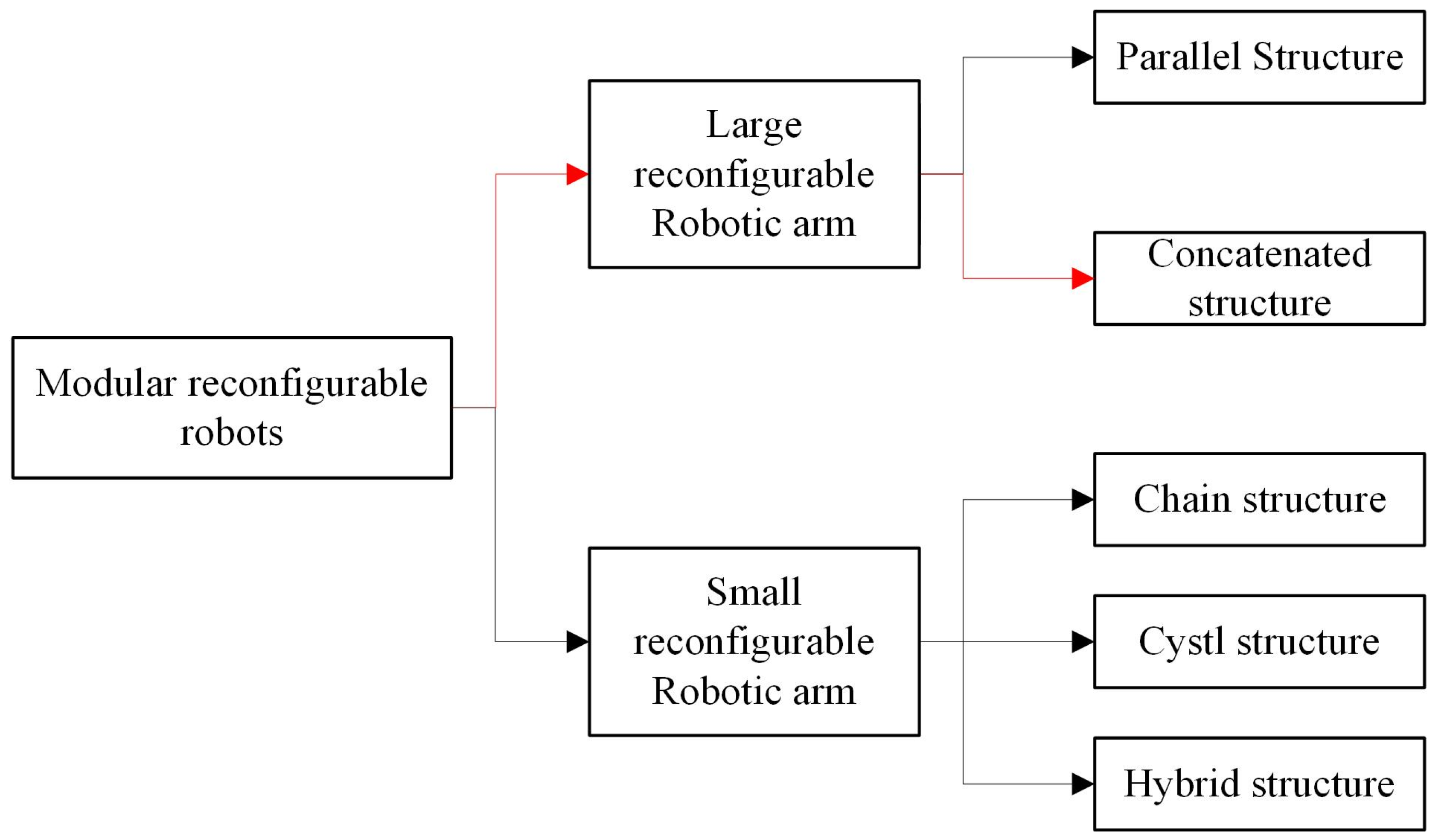
This study focuses on the problem of determining a robotic arm’s ideal configuration for various jobs and environmental variables in a genuine industrial setting. The tandem structure of a large-scale reconfigurable manipulator arm [9] is considered in the paper. (Figure 1 Branch shown by red arrow). The objective is to obtain the optimal construction of the robotic arm model with high calculation efficiency while the cost of the reconfiguration model can be minimized.
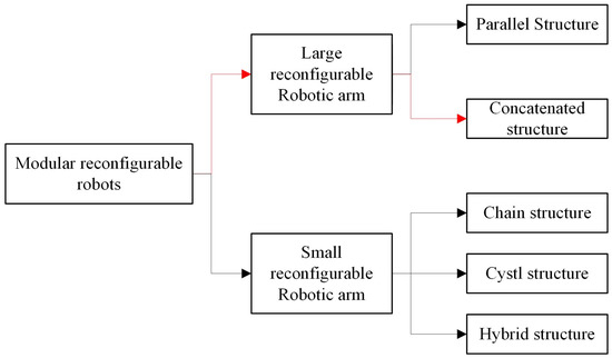
Figure 1.
Categories of Modular Reconfigurable Robots.
In this study, a DDQN-based modular robotic arm reconstruction algorithm with improved preferred experience replay idea is proposed, so that the algorithm can make effective use of the historical experience to ensure the algorithm fails to achieve the local ideal result [10,11]. The main contributions of this paper include:
- (1)
- The DDQN-based algorithm for designing the optimal modular robotic arm configuration is constructed in this paper, which enhances the modular robotic arm’s performance compared to the traditional DQN algorithm. This DDQN-based algorithm selects the best action by assessing the value of each action in the current state using a main network and a target network. The target network assesses the action values for future states, whereas the main network computes the action values in real-time for the current state. This algorithm can assess the value of actions more precisely and avoid the overestimation issue by using this dual network topology.
- (2)
- To better utilize historical experience, this article has improved the experience replay mechanism and introduced priority experience replay technology based on SumTree. This replay mechanism can efficiently pick out crucial experiences for training, keep the algorithm from entering local optima later in the process, and increase the convergence speed and training effectiveness compared by employing the results of the Sumtree as the storage structure for the memory bank.
- (3)
- A robotic arm module library was developed utilizing SOLIDWORKS 2019 software, enabling the integration of a diverse series of robotic arms. Subsequently, the model was converted into a URDF robot description file in XML format using the SW2URDF plug-in, and simulation experiments were conducted on the PyBullet simulation platform.
The experimental results demonstrate that the improved double DQN algorithm is applied to the reconfiguration task of a modular robotic arm, which is intended to perform operations under different environmental constraints. Simultaneously, the goal of searching for configurations with lighter and fewer joint modules can be reached, allowing the robotic arm configuration to have a lighter and more compact structure.
2. Problem Formulation
2.1. Modelling of Robotic Arm Modules
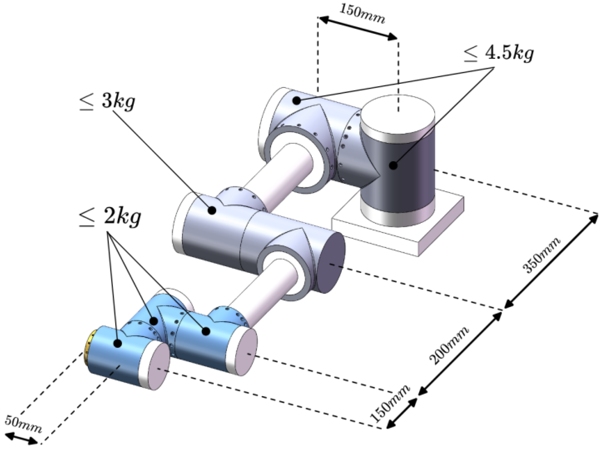
Building a library of robotic arm modules can improve the efficiency of design, increase the reconfigurability of the system, as well as simplify the maintenance and update process, which leads to greater convenience and flexibility in the development and application of robotic arms. In the study, three specifications of joint modules are usually used: shoulder joint, elbow joint, and wrist joint. At the same time, the mass of each joint is pre-assigned, in which the wrist joint does not exceed 2 kg, the elbow joint does not exceed 3 kg, and the shoulder joint does not exceed 4.5 kg. The predefined parameters of the tandem robotic arm are shown in Figure 2. The three joint specification size parameters set in this paper are shown in Table 1.

Figure 2.
Predefined parameters for tandem robotic arms.

Table 1.
Predefined parameters for tandem robotic arms.
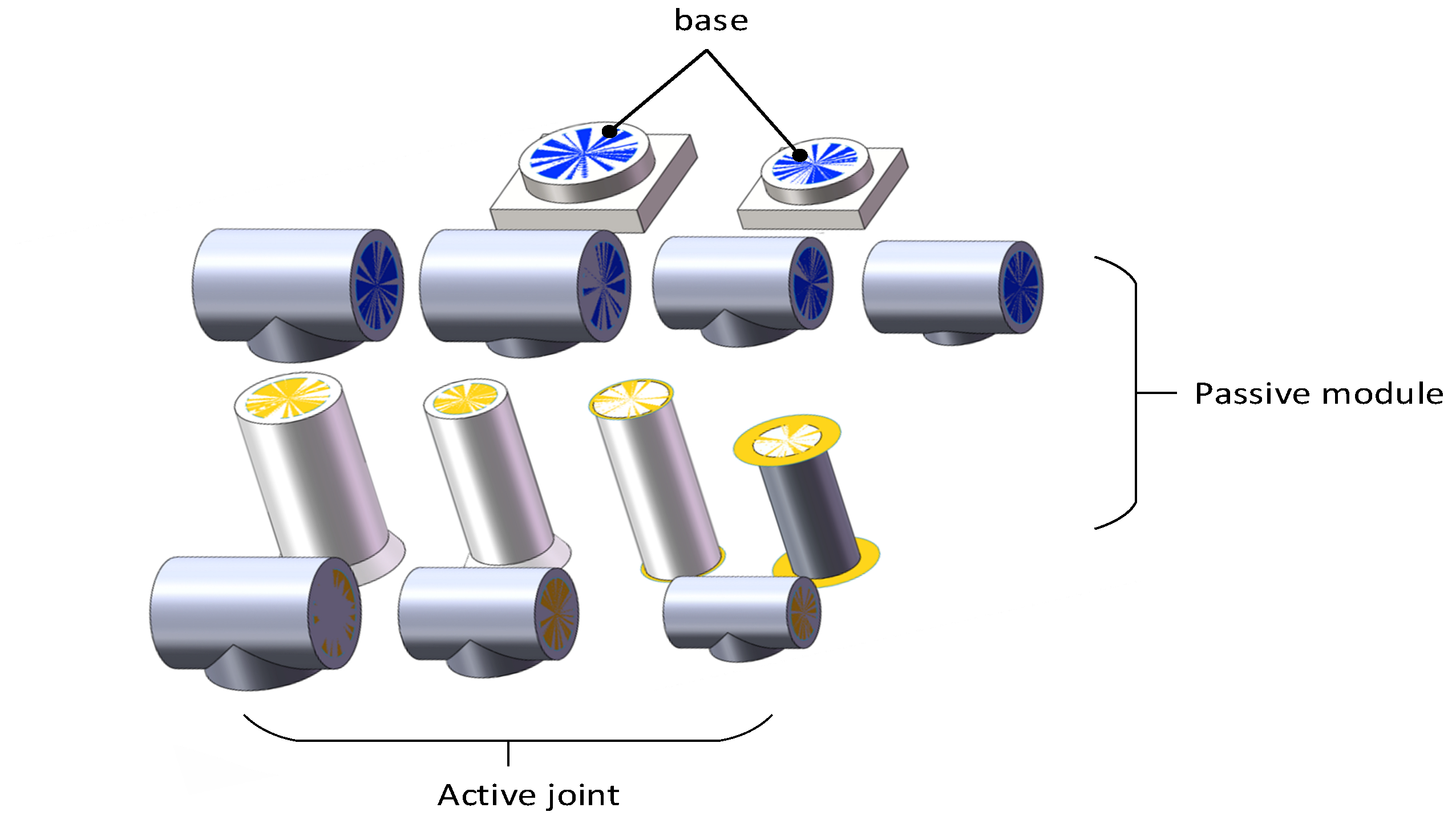
A small module library was created by using the SolidWorks 2019 software. The library contains a total of thirteen modules, including two models of base modules, three models of active modules, and eight passive modules with different sizes and shapes, as shown in Figure 3. At the same time, the SW2URDF plug-in in SolidWorks was used to convert these models into URDF (Unified Robot Description Format) robot description files in XML format, so that the relevant training environment could be built in Pybullet simulation 3.1.0 software to conduct simulation experiments.

Figure 3.
Robotic Arm Small Module Library.
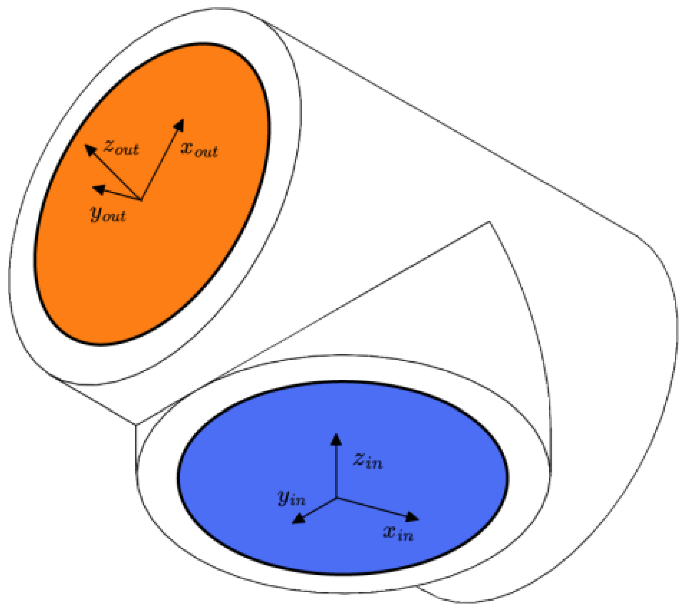
Each joint module in this paper has a standard input/output interface, using the characteristics of the URDF file. The “virtual linkage” can be defined by putting the input/output interface information in its corresponding URDF file [12]. For example, the T-joint module is shown in Figure 4, where the orange “virtual links” indicate the output interfaces and the blue “virtual links” indicate the input interfaces. In addition, the coordinate system definition rule of URDF requires that the geometry of the “virtual links” is defined in the URDF file of each “virtual link”. The rules for defining the URDF coordinate system require that a coordinate system be established at the geometric center of each “virtual link”, with the axes of the coordinate system parallel to the direction of the normal to the surface of the “virtual link” (in the direction of the z-axis). The axis of the coordinate system points outward for output interfaces, while the axis of the coordinate system points inward for input interfaces in Figure 4.

Figure 4.
Coordinate system of the T-joint module.
To assemble multiple modules into a complete robot, it is necessary to define the assembly rules between URDF files. Taking the assembly between two T-joint models as an example, the assembly is completed when the output coordinate system {out} of module {i-1} coincides with the input coordinate system {in} of module {i}. As shown in Figure 5, the red arrow indicates the path, i.e., the output “virtual link” (orange) of module {i-1} is connected to the input “virtual link” (blue) of module {i} to complete the assembly.
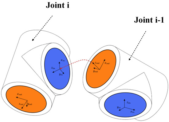
Figure 5.
Assembly rules for modules.
2.2. Modular Robot Design Based on Reinforcement Learning
The design methodology in this paper aims to generate the optimal tandem robotic arm configuration to perform the task based on the given robotic arm module library and the task in different scenarios. The optimal configuration is determined based on factors including the number of modules and mass of the complete robotic arm. The tandem robotic arm’s construction procedure is depicted in Figure 6. In this process, the base module is added first, the configuration is formed by adding new joint modules to the base module, the new configuration is formed by continuing to add modules from the configuration library to the configuration , and the configuration that ends only with the end-effector module is defined as the complete configuration.

Figure 6.
Reconfiguration process diagram of the tandem robotic arm.
The configuration design problem of a modular tandem robotic arm can be modeled and resolved by using the Finite Markov Decision Process (MDP). Set up a quaternion structure, where S denotes the set of state values of the environment, defined by the set of robotic arm configurations. The action space A is defined by the available robot module library. R denotes the reward value obtained by adopting an action in a particular state, and E (Expected value) represents the mean of random variables. At each moment t, the reinforcement learning intelligence must perform an action, which means selecting the index value of a module and adding the corresponding module to the current configuration . The only part of the state that changes is the configuration , so the state at the next moment depends only on the previous moment’s state and the action of adding the module. represents the policy function. At this point a new state is produced, containing the new configuration and a reward from the environment . The expected payoff of the reward that the agent receives for choosing an action in the state is (Conformity applied in Equation (1) to Equation (15) is specified in Table 2 in terms of interpretations and units.):
The discount factor is used to calculate the cumulative reward R. The state value function of the policy taken at state is defined as:
Based on the policy and the action , the value function of the action in the state is:
The algorithm uses reinforcement learning strategy to estimate the optimal state-action-value function , which can be defined by the Bellman optimality equation:
2.3. Deep Reinforcement Learning
Q-learning is a reinforcement learning algorithm based on value iteration, which employs a tabular method to compute the valuation of Q-values corresponding to each possible state-action pair. In modular robotic arm configuration design, the high-dimensional continuous state and action space make the traditional Q-value estimation based on the table method difficult. The Deep Q-Network method was employed to solve this problem [13]. The space complexity issue of keeping a Q-table is avoided by fitting the Q-value function through a neural network, which may directly input the states and output the Q-value of each action. At the same time, the nonlinear fitting ability of deep neural networks can better approximate complex Q-value functions.
Traditional DQN employs two neural networks with the same topology but different parameters. One network is used to update the parameters in real time while the second network is utilized to update the target Q-value. The updating formula for the target Q-value is:
Despite this, standard DQN algorithms select the greatest Q value from the target Q network for each action, which is prone to choose the overstated value and ultimately cause the overestimation issue. The Deepmind team proposed DDQN in 2015 to solve this problem by independently training two separate Q-networks [14]. Double DQN introduces two separate neural networks (which also have the same structure and different parameters as DQN): one for selecting the actions (the action selection network) and the other for evaluating the value of the selected actions (goal network). Instead of using the target network directly to select the maximum action value for the next state when calculating the target Q value, the action selection network is used to select the action:
This action is used as the action for calculating the target Q value, and the selection of the optimal action is accomplished using the target network. The calculation of the target Q in Double DQN is shown in Equation (7):
In this paper, the principle of DDQN is applied to the modular robotic arm configuration design to solve the high dimensional and complex problem of robotic arm module reconfiguration.
3. Method
3.1. Double DQN for Module Selection
The paper aims to find the optimal configuration of a robotic arm for different tasks to reach the specified task point accurately. The robotic arm consists of a set of modules with module index . As a result, the problem of configuration optimization of a modular reconfigurable robot can be formulated as selecting a sequence of modules. The configuration consisting of these modules in order can perform the given task. The metrics and functions to assess the optimality of the robotic arm in this paper are given below.
3.1.1. Target Point Accessibility
The workspace objective (positional pose) is described by the set , where denotes the coordinates of the end-effector in space and denotes the orientation of the end-effector. A sequence of modules C is selected, and to evaluate whether the configuration can reach the given objective. The position error and attitude error are set according to the joint accuracy of the robot. and denote the output postures of the inverse kinematics solution corresponding to the positive kinematics for the given objective. The “reachability” function of the configuration C for a given pose is defined by the equation:
3.1.2. Terminal State
When the added module is an end-effector, the arm reaches the terminal state, and the environment returns a reward given by the “reachability” function in equation, which is evaluated only for complete configurations. Meanwhile, a penalty of −1 is returned for configurations that do not have an end-effector added to the terminal state (the maximum number of modules in this paper is set to be Nmax = 15).
3.1.3. Constraints
As affected by the mechanical structure joint driving ability and other factors, the joint angle of each joint of the robotic arm has a certain constrained range, which is defined as:
where is the inverse kinematics solution of the reconfigurable robotic arm, and and are the joint angles’ minimum and maximum values, respectively.
3.1.4. Optimal Configuration
The ultimate goal of evaluating the robotic arm configuration is to find the optimal configuration . It is desirable to have a robot with fewer drive modules and a lighter mass. The resulting definition of the objective function is given by the equation:
where denotes the number of drive joints in a given robotic arm configuration and denotes the total mass of the configuration . and are the weighting factors for the number of modules and the total mass of the configuration , respectively, to achieve a proper trade-off between multiple objectives. The optimal configuration is defined as given by the equation.
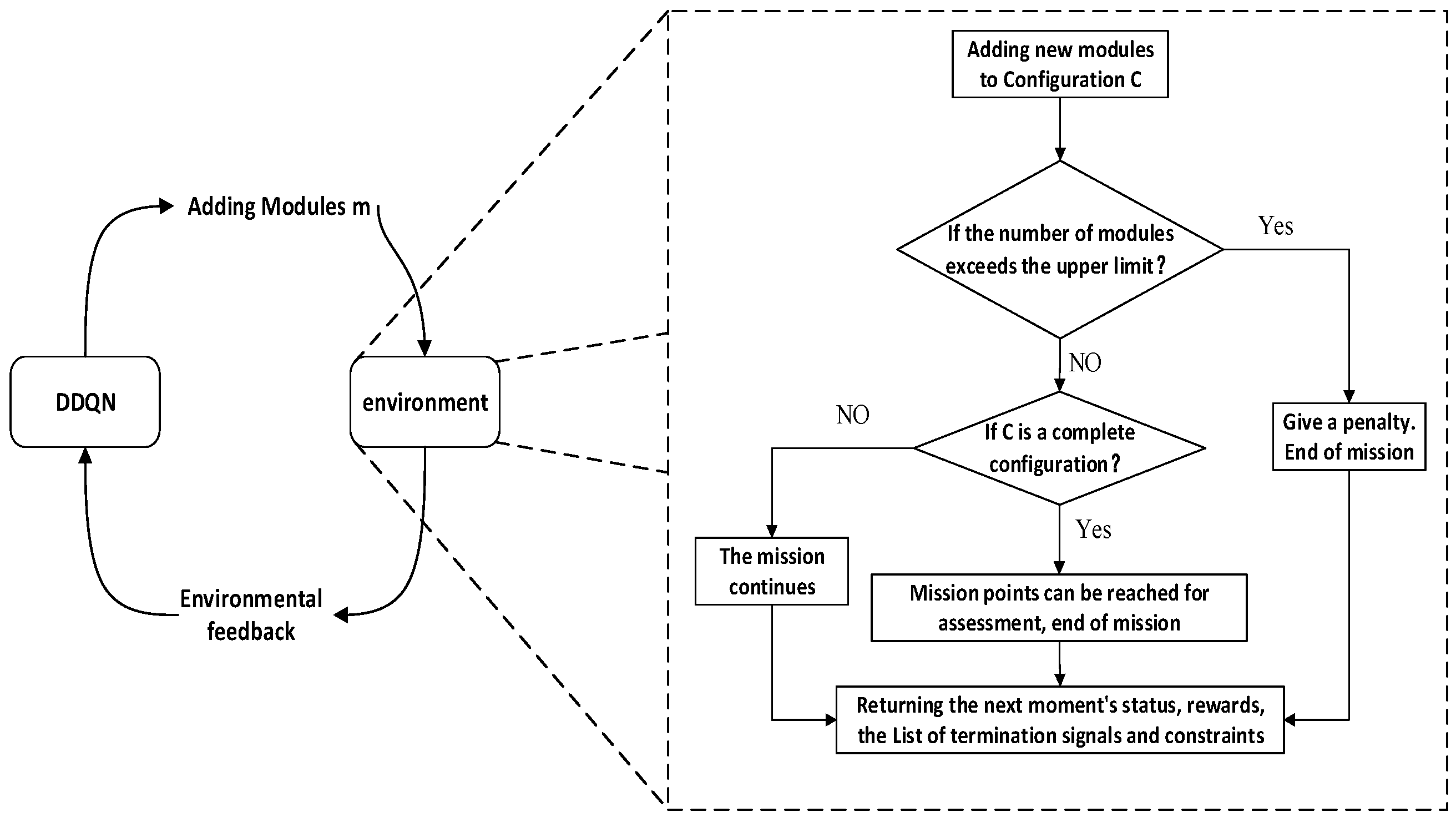
Based on the above metrics and functions, the training interaction process is shown in Figure 7, where the DDQN-based method selects the next robot module to be assembled based on the list of states and submodule constraints provided by the simulation training environment. The environment immediately adds the module to the current configuration and returns the state, reward value, termination value, and list of submodules for the next moment.
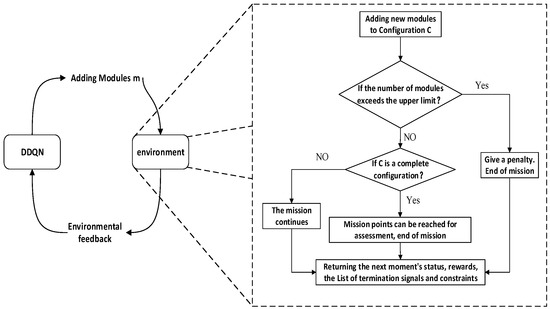
Figure 7.
Flowchart of optimal configuration design.
3.2. Modified Double DQN with SumTree
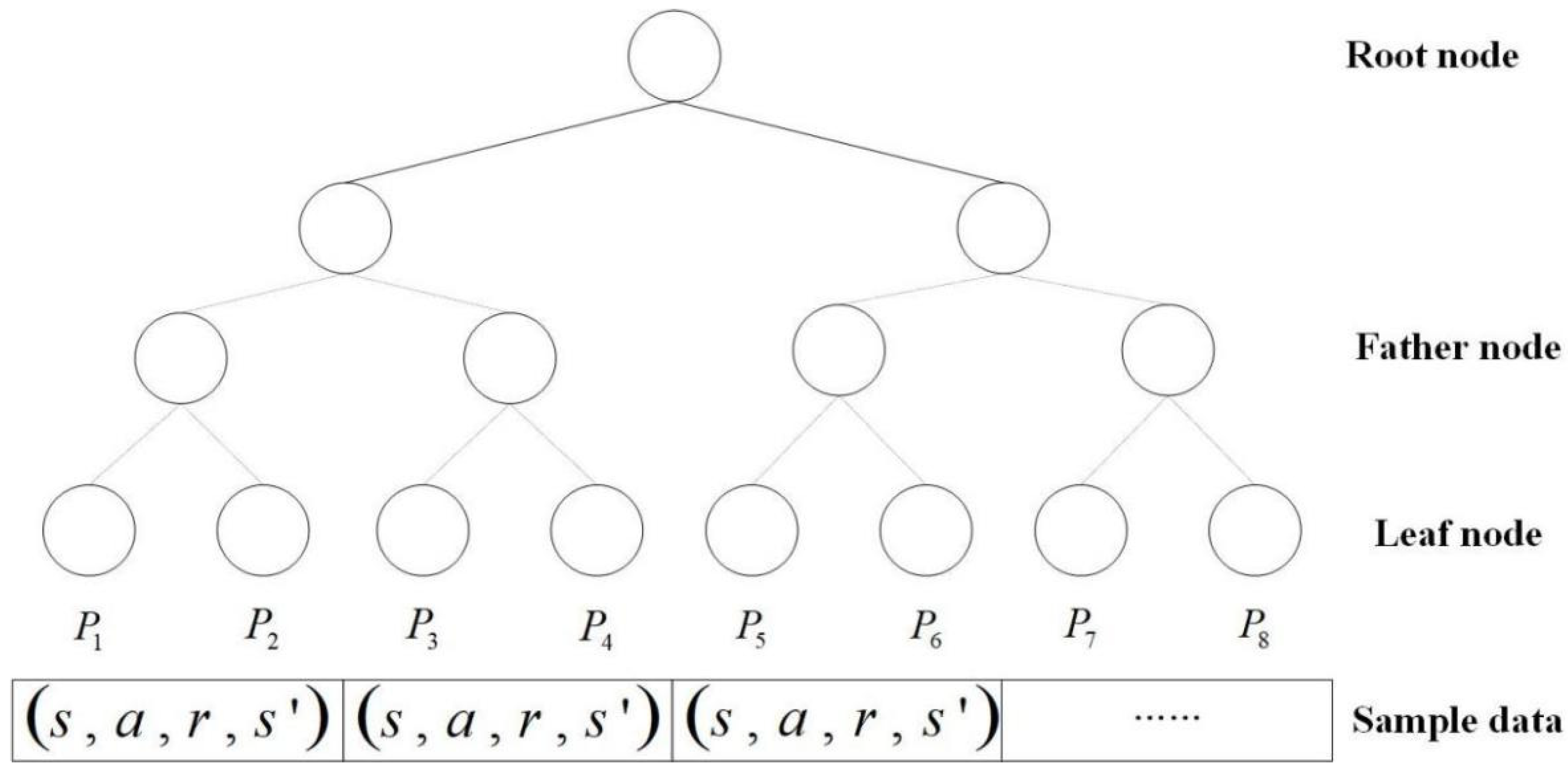
The traditional experience replay mechanism blocks the relevance of the training samples, and the uniform sampling is not conducive to filtering out the quality samples, which is not beneficial to the convergence of the algorithm. In addition, the traditional sampling method needs to sort all the samples, which requires much computation consumption. For better sampling, this paper adopts the prioritized experience replay method based on the SumTree [15]. SumTree is a special binary tree data structure, as shown in Figure 8. There are four layers of node structure in a SumTree, the top node is called the root node. The middle two rows are called the parent nodes and the bottom row is called the leaf node. All empirical samples are stored in the leaf nodes, which also store the priority of the samples.
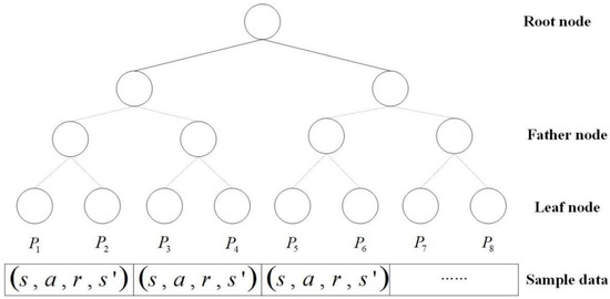
Figure 8.
Sumtree structure diagram.
The temporal difference error (TD error) determines the priority of the samples in the SumTree sampling. The value of the TD error shows the strength of the neural network’s backpropagation effect. The priority of experience and its probability of selection are given as
where is a very small number that prevents the probability from being equal to 0, and is the experience’s priority. is the probability that the sampling experience is selected. is a hyperparameter that controls the sampling preference in uniform and greedy sampling.
To compensate for the bias in value estimation, a significance sampling coefficient is employed:
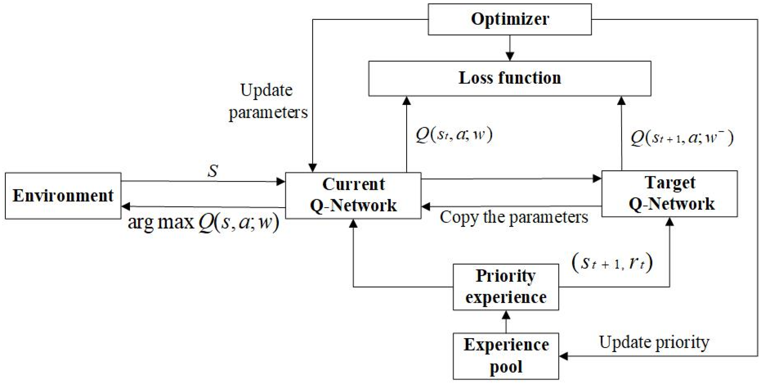
Notably, the quantity of experience needed for learning is decreased by using the developed priority experience replay mechanism. The model’s training time and the number of training iterations can be reduced. The schematic of the proposed DDQN-based algorithm is given in Figure 9.
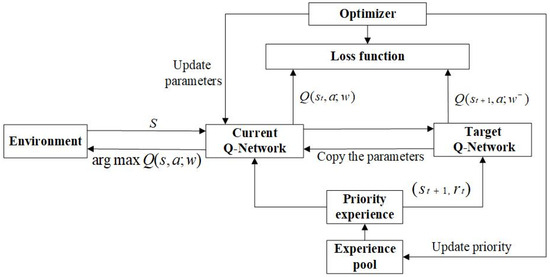
Figure 9.
Schematic of the DDQN algorithm with prioritized experience replay.
Table 2.
Explanation of the symbols.
Table 2.
Explanation of the symbols.
| Nomenclature | |||
|---|---|---|---|
| Current configuration of robotic arms | Maximum value of joint angle | ||
| New robotic arm configuration | Optimum arm configuration | ||
| The set of state values of the environment | Number of joints | ||
| Action space | Total mass of joints | ||
| Reward returns | Weighting factor for number of modules | ||
| Policy function | Weighting factor of module mass | ||
| Discount factor | Priority of experience | ||
| Expected value | Probability of sampled experience being selected | ||
| Workspace target point | Importance sampling factor | ||
| Position error | Controlling sampling priority in uniform and greedy sampling | ||
| Attitude error | Experience pool size | ||
| Minimum value of joint angle … rad | Hyperparameters to counteract the effect of priority experience replay on convergence results | ||
3.3. Modular Robotic Arm Algorithm Based on Improved DDQN Algorithm
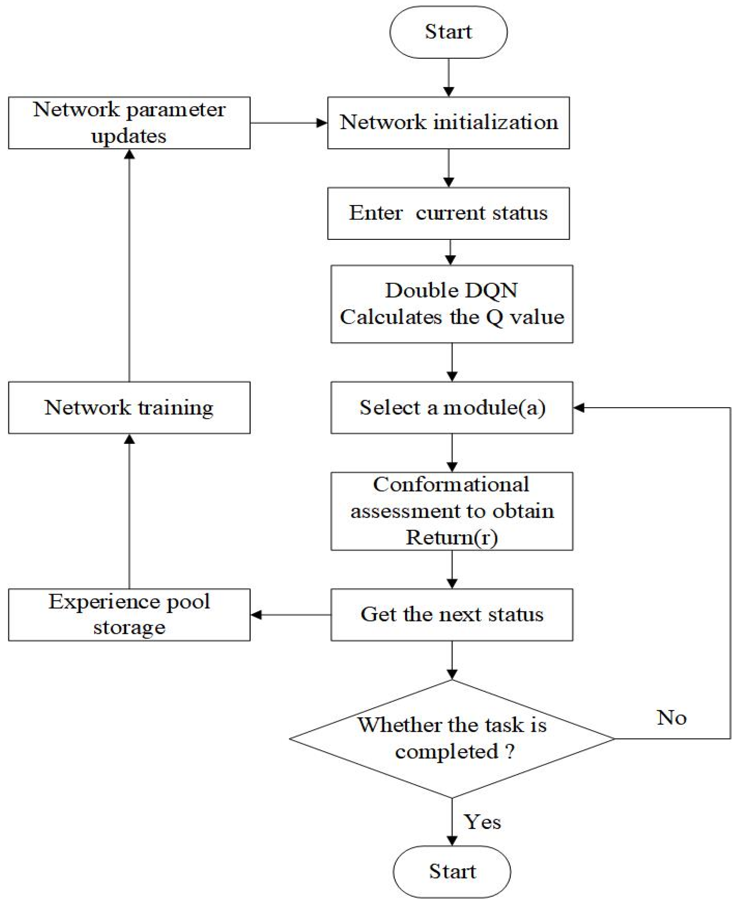
The DDQN algorithm with preferred experience replay is applied to obtain the optimal modular robotic arm configuration in this paper, with the flow of the algorithmic model shown in Figure 10. The algorithm adopts the current configuration’s state information, constraints, and reward signals as the inputs to obtain the value corresponding to the selection of each module. A module is selected using the greedy strategy. The obtained new configuration would be evaluated, and the reward r is then obtained. The value is updated by the return value, which would determine the module to be selected for the next step. Then, the four variables mentioned above are deposited into a quaternion of samples . A certain batch of samples is taken from the sample pool according to the priority weights to train the neural network and update the network parameters. Then the module selection is carried out again and the cycle is repeated until the terminal state is reached. Through this iterative training process, the algorithm can continuously optimize the configuration selection strategy and find the optimal robotic arm configuration under different tasks. The structure and iterative process of this neural network is shown in Figure 11.
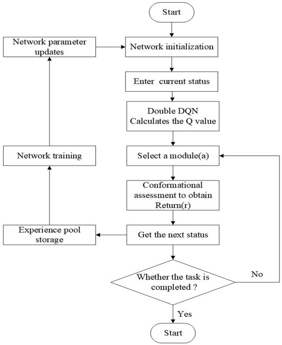
Figure 10.
Flowchart of the application of Double DQN algorithm based on priority experience.
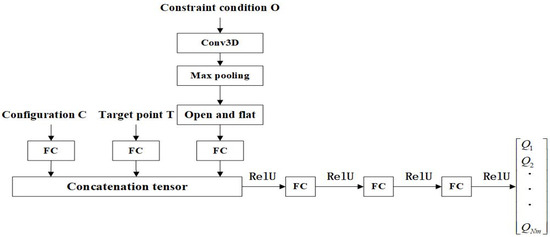
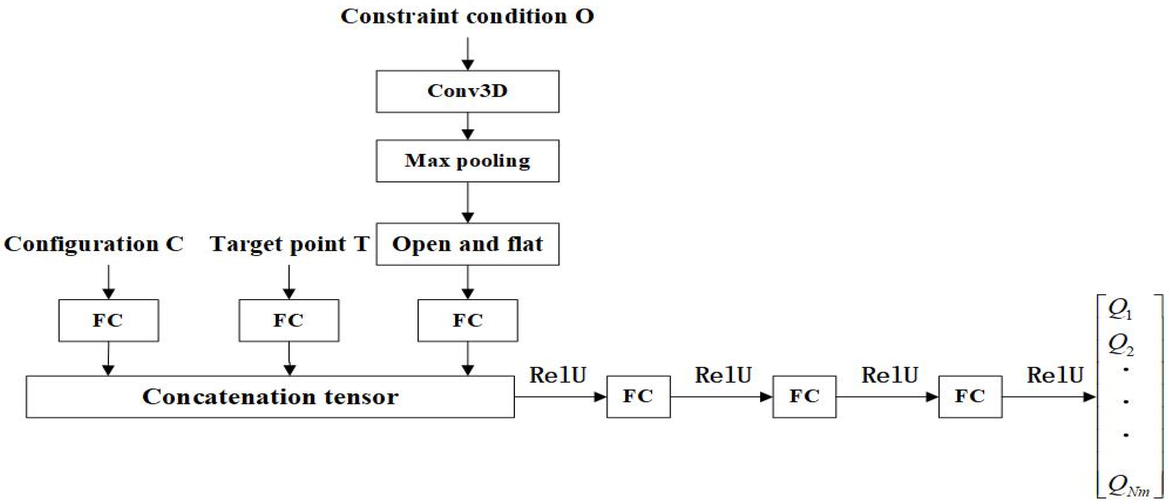
Figure 11.
Schematic diagram of neural network structure.
The pseudo-code of this algorithm is shown in Algorithm 1.
| Algorithm 1: Double DQN with proportional prioritization |
| 1: Input: 2: Result: optimal configuration 3: Initialize replay memory 4: Set replay period , budget T, step size , minibatch and size , exponents 5: Observe Initial state () and choose an action 6: for t = 1 to T do 7: Observe in H and set its priority to 8: Store transition 9: if mod then 10: for i = 1 to do 11: Sample transition 12: Compute the importance sampling weight 13: Compute TD-error 14: Update transition priority 15: Accumulate change in cumulative weight 16: end for 17: Update weights , reset 18: At times copy new weights into the target network 19: end if 20: Choose an action 21: end for |
The input to the neural network consists of the current configuration C, the workspace T, and the constraints O. These three tensors are concatenated by the Concatenate operation after a layer of fully connected layers to generate a combined input tensor. The three fully connected layers are activated using ReLU as an activation function. The ReLU activation function is applied after the output of each layer by setting the negative values to zero and keeping the positive values constant. The final output is a state-behavior value for each module Q. The state-behavior value Q is used to guide the decision-making process, helping the agent to select the next robot module to be assembled and to maximize the cumulative rewards within the given constraints. The structure of the neural network is described in Figure 11.
4. Numerical Experiments
4.1. Simulation Environment
In this paper, a custom simulation environment for robot configuration optimization was created using the OpenAI gym reinforcement learning platform and the PyBullet physics engine. The simulation environment defines the obstacle (left) and the task space (right). The obstacle consists of a cube with a prism length , and task space is defined as a space containing the possible locations of the obstacle and the target in Figure 12.
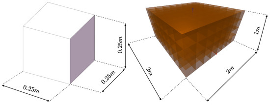
Figure 12.
Obstacles and Task Space in Simulated Environments.
4.2. Experimental Parameter Setting
The code is deployed on the Aliyun ECS cloud server for training and the experimental environment is shown in Table 3.
Table 3.
Experimental operating environment.
For a comparative study, the performance of the proposed algorithm with DDQN and preferred experience replay was compared with that of the traditional DQN algorithm. Both algorithms use the same hyperparameters, which are shown in Table 4.
Table 4.
DDQN algorithm hyperparameters.
The parameters that can be adjusted in the simulation environment are shown in Table 5, where the reference values are also the parameters used in the training environment in this paper:
Table 5.
Simulation environment adjustable parameters.
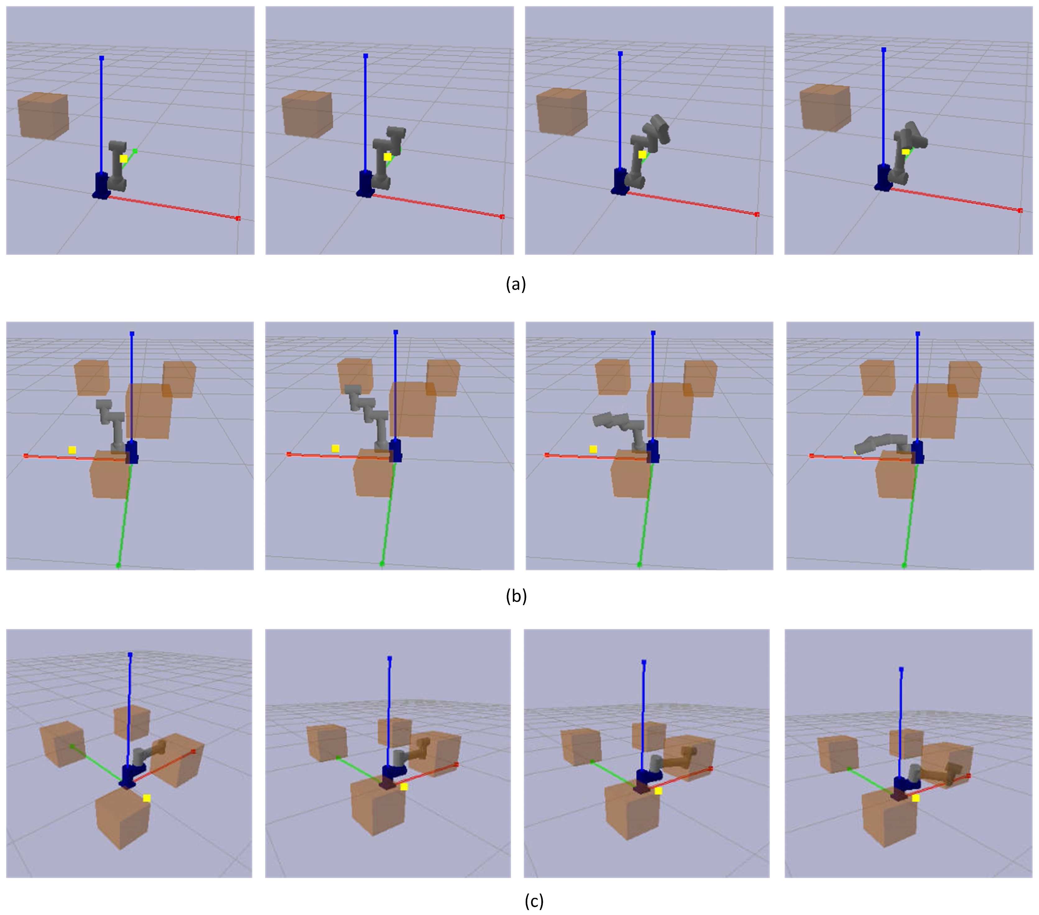
The PyBullet simulation engine was used to construct the training environment. The simulation runtime interface is illustrated in Figure 13. It can be seen that a multi-degree-of-freedom robotic arm is generated at the origin, and the yellow dots indicate randomly generated target points, while orange cubes indicate obstacles. Figure 13a depicts the robotic arm’s role configuration when it successfully reaches the goal point but encounters no obstacles. The robotic arm’s arrangement that effectively avoids obstacles and reaches the target position is depicted in Figure 13b. Figure 13c shows a failed operation of the robotic arm, which fails to reach the target point.
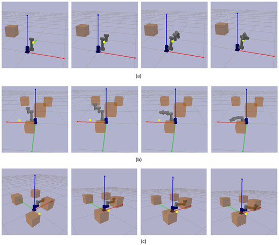
Figure 13.
Simulation runtime interface. (a) The robotic arm configuration successfully reached the target point, but random obstacles did not hinder it. (b) The robotic arm configuration successfully achieves the target point while avoiding obstacles. (c) Configuration failed to reach the destination.
5. Results and Discussion
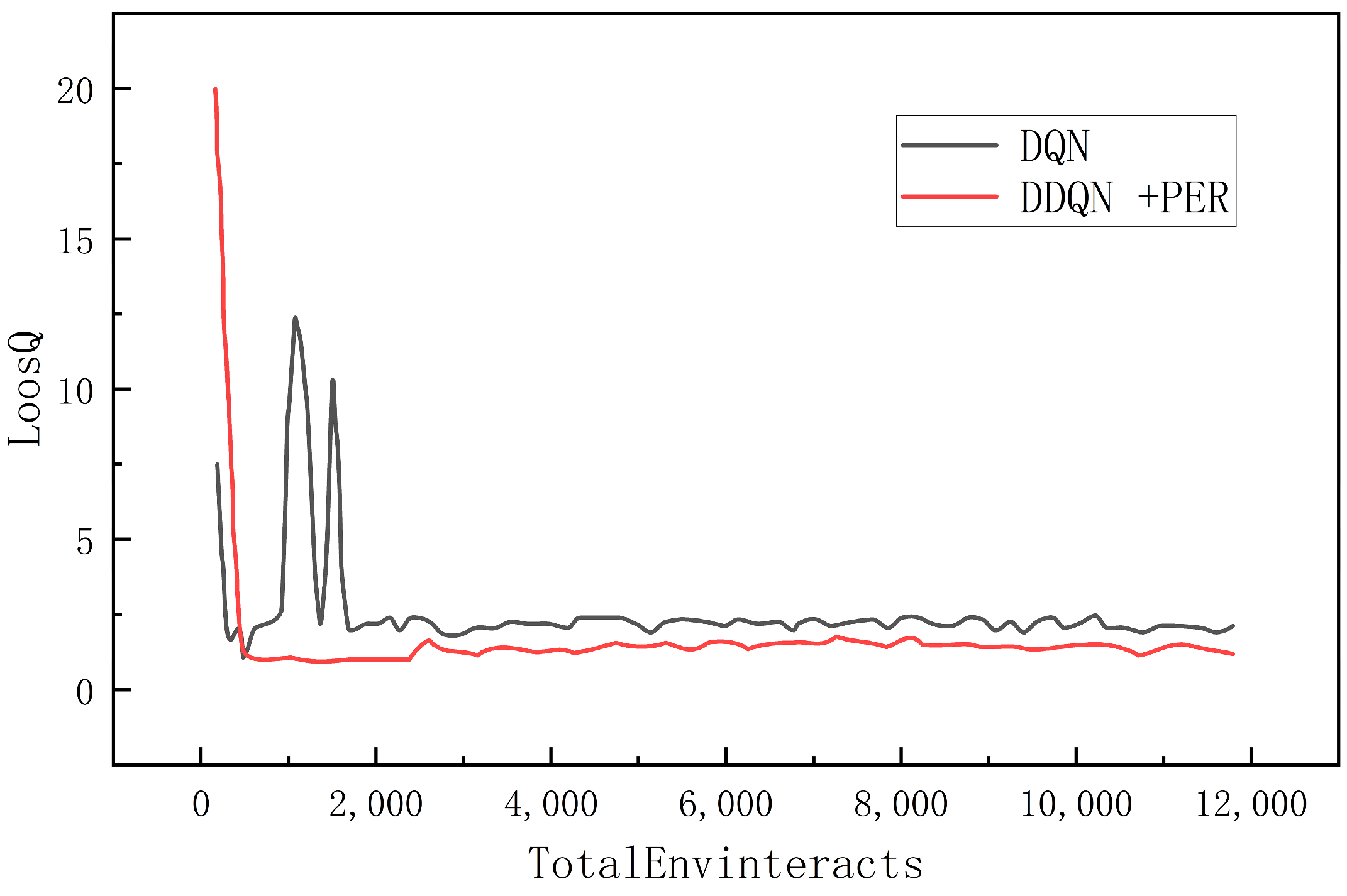
This experiment was conducted for a total of 80 epochs, each containing 150 interactions. Two different deep reinforcement learning algorithms, the DQN algorithm and the DDQN algorithm, which combine features of both deep learning and reinforcement learning algorithms, were implemented in the same training environment. The variation of the loss function is plotted in Figure 14. It is shown that both algorithms were able to reach a state of convergence after a certain number of training rounds. The traditional DQN algorithm starts to converge when the number of training steps approaches 1900 steps. There exist large loss fluctuations before this point. The improved DDQN algorithm converges faster and can reach a stable convergence around 500 steps, with its average loss value remaining below 2.5. Under the same training environment, the DDQN algorithm shows a faster convergence speed and better stability than the traditional DQN algorithm, and its average loss value is also smaller. This indicates that the improved algorithm learns and optimizes the Q-value function more efficiently during the training process, which enhances the learning ability and performance of the agent.

Figure 14.
Loss Function Comparison.
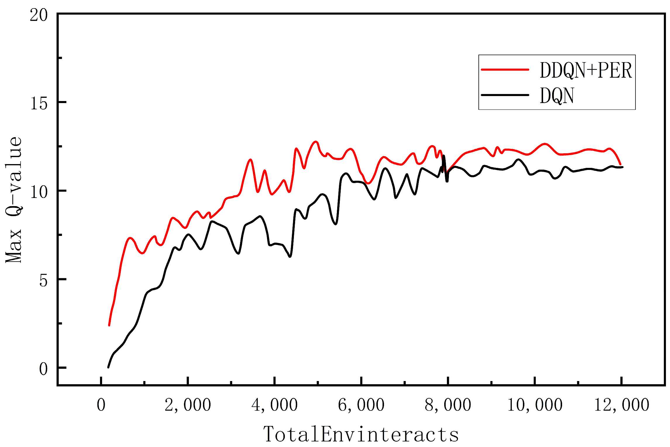
Time histories of the greatest Q value for every selection in both methods are shown in Figure 15, which demonstrates that the maximum Q value for both algorithms follows a similar trend and converges to close to 12 after roughly 8000 iterations. However, the average value of the maximum Q value of the DQN algorithm after convergence is 11.689, and the same index for the improved DDQN algorithm is 11.302, which indicates that the DDQN algorithm successfully mitigates some of the over-estimation. The algorithm is more accurate in estimating and updating the Q value function in the training process, which improves the performance and stability of the algorithm.

Figure 15.
Maximum Q Comparison.
The average reward values obtained by the two algorithms are compared in Figure 16. It can be observed that both curves would reach stable states after more than 30 training rounds. The average reward value of the DDQN algorithm converges near about 9 and the total average reward over 80 training rounds is 485.026. Meanwhile, the average reward value of the DQN algorithm would converge to about 8 and the total average reward is 378.511. In addition, the DDQN algorithm produced a higher average reward values than the DQN algorithm in the vast majority of cases. This suggests that the DDQN algorithm learned a better policy and was able to select more efficient actions in the environment, thus increasing the overall reward of the agent. This also validates the effectiveness of the improved DDQN algorithm and further demonstrates its better learning ability and adaptability relative to the traditional DQN algorithm.
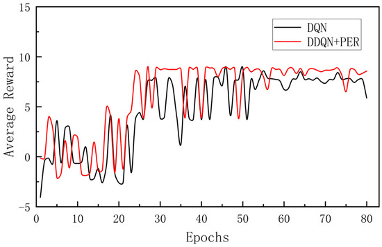
Figure 16.
Comparison of average reward values.
The purpose of the experiments is to evaluate the performance of the proposed algorithm in resolving the modular configuration design problem of robotic arms. In the simulations, a total of 50 groups of random tests were generated, with each group of targets containing a grid of up to five random obstacles. In each group, a target point was randomly generated through a normal distribution, and the configuration that successfully reached the target point was defined as the feasible configuration. The following performance indexes are considered.
- (1)
- I1: The probability of successfully finding an optimal configuration;
- (2)
- I2: Average module mass of feasible configurations;
- (3)
- I3: The average number of modules in a feasible configuration;
- (4)
- I4: Average time to find a feasible configuration;
The results of the comparative experiment are shown in Table 6:
Table 6.
Comparison Test Results.
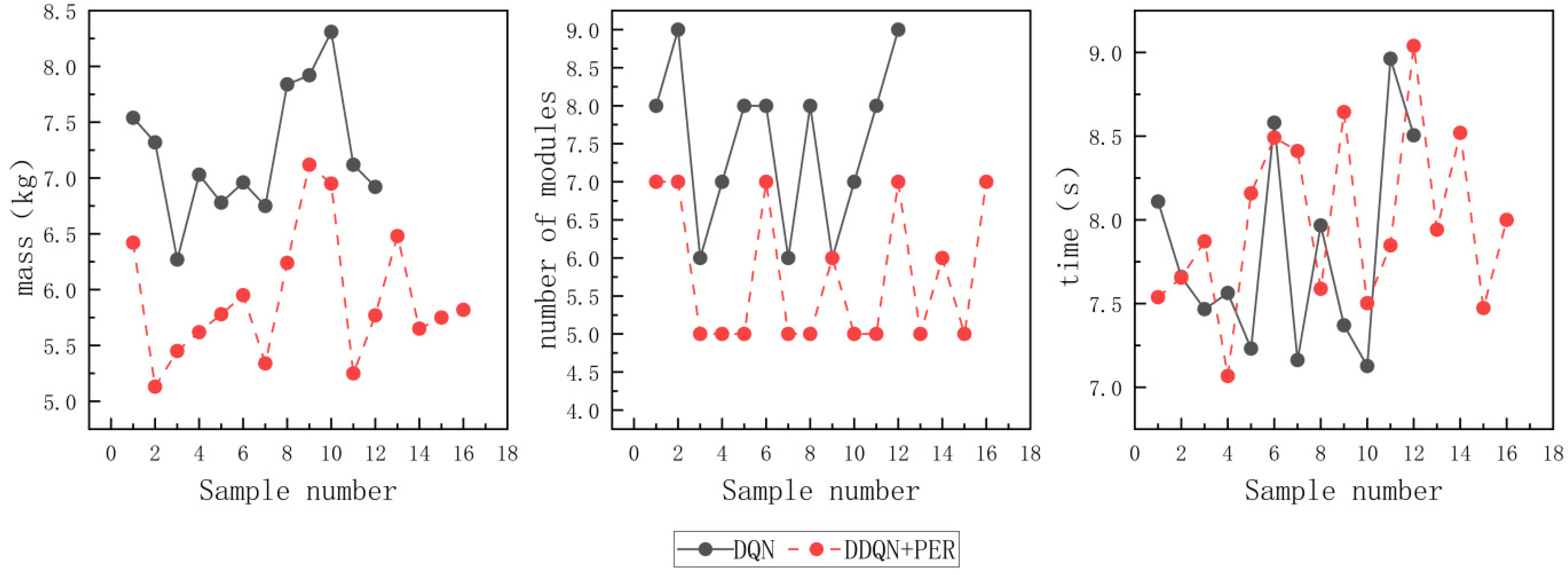
The traditional DQN algorithm succeeded in finding complete configurations in 12 out of 50 sets of tests, while the proposed algorithm found 16 sets of complete configurations. It can be determined that the average mass of complete configurations obtained by the proposed algorithm in this paper is about 5.92 kg, and I2 for the traditional DQN algorithm is about 7.23 kg. The method in this paper decreases the average mass of robotic arm modules by about 18.11%. As for I3, the algorithm proposed in this paper has 1.74 fewer average modules compared to the traditional DQN algorithm. It is shown that the average time to find a feasible configuration for the two algorithms are comparable. The comparison of performance indexes is shown in Figure 17.
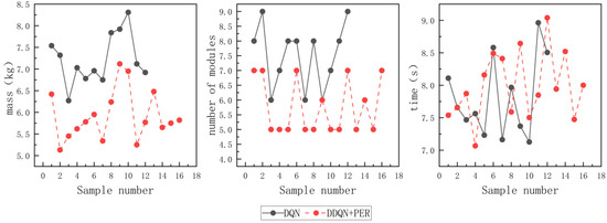
Figure 17.
Comparison of performance indexes.
Through the above comparative test results, it can be concluded that compared to the traditional DQN algorithm, the algorithm proposed in this paper has a higher probability of successfully finding feasible configurations, with less mass and fewer number of modules. To conclude, the algorithm in this paper is capable of finding more feasible configurations that have lighter and more compact structures, which could lead to higher efficiency and performance in practical applications.
6. Summary
In this paper, a DDQN-based configuration design algorithm with prioritized experience replay for modular robotic arms is proposed, aiming to resolve the conflict that exists between diversity and economy in robotic arm design. The algorithm is improved by making improvements in terms of task customization and robot economics, and comparative experiments are conducted with the traditional DQN algorithm. The results show that the algorithm can reduce the risk of overestimation of the Q-value and improve the convergence performance of the algorithm by prioritizing the empirical replay mechanism. This enables the modular robotic arm to achieve a higher success rate in the reconfiguration process while also improving the quality of the optimal configuration to adapt to complex and changing production environments and task requirements.
Future work could consider applying the algorithm to real robotic arm modules through transfer learning and other methods to achieve modular robotic arm reconstruction in real scenarios. A crucial aspect for addressing specific real-world applications lies in the effective translation of physical mechanisms into mathematical simulation models, with digital twin technology serving as a valuable resource. This will further validate the feasibility and effectiveness of the algorithm and explore its potential and limitations in practical applications.
Author Contributions
Conceptualization, Z.D. and H.T.; methodology, H.T.; software, H.T.; validation, Z.D. and H.T.; formal analysis, Z.D.; investigation, H.T.; resources, C.Z.; data curation, Z.D.; writing—original draft preparation, Z.D. and H.T.; writing—review and editing, C.Z. and R.S.; visualization, H.W.; supervision, R.S.; project administration, R.S.; funding acquisition, R.S. All authors have read and agreed to the published version of the manuscript.
Funding
This research was funded by the Basic Scientific Research Project of China (Grant no. JCKY2020903B030982).
Data Availability Statement
Data are contained within the article.
Conflicts of Interest
The authors declare no conflict of interest.
References
- Liu, S.B.; Althoff, M. Optimizing performance in automation through modular robots[C/OL]. In Proceedings of the 2020 IEEE International Conference on Robotics and Automation (ICRA), Paris, France, 31 May–31 August 2020; pp. 4044–4050. [Google Scholar]
- Desai, R.; Safonova, M.; Muelling, K.; Coros, S. Automatic design of task-specific robotic arms. arXiv, 2018; arXiv:1806.07419. [Google Scholar]
- Izzo, D.; Märtens, M.; Pan, B. A survey on artificial intelligence trends in spacecraft guidance dynamics and control. Astrodynamics 2019, 3, 287–299. [Google Scholar] [CrossRef]
- Luo, H.; Li, M.; Liang, G.; Qian, H.; Lam, T.L. An obstacle-crossing strategy based on the fast self-reconfiguration for modular sphere robots. In Proceedings of the 2020 IEEE/RSJ International Conference on Intelligent Robots and Systems (IROS), Las Vegas, NV, USA, 25–29 October 2020; IEEE: New York, NY, USA; pp. 3296–3303. [Google Scholar]
- Whitman, J.; Bhirangi, R.; Travers, M.; Choset, H. Modular robot design synthesis with deep reinforcement learning. In Proceedings of the AAAI Conference on Artificial Intelligence, Vancouver, British Columbia, 20–27 February 2024; Volume 34, pp. 10418–10425. [Google Scholar]
- Hessel, M.; Modayil, J.; van Hasselt, H.; Schaul, T.; Ostrovski, G.; Dabney, W.; Horgan, D.; Piot, B.; Azar, M.; Silver, D. Rainbow: Combining improvements in deep reinforcement learning. In Proceedings of the AAAI Conference on Artificial Intelligence, New Orleans, LA, USA, 2–7 February 2018; Volume 32. [Google Scholar]
- Haarnoja, T.; Tang, H.; Abbeel, P.; Levine, S. Reinforcement learning with deep energy-based policies. In Proceedings of the International Conference on Machine Learning, Sydney, Australia, 6–11 August 2017; pp. 1352–1361. [Google Scholar]
- Zhai, P.; Zhang, Y.; Shaobo, W. Intelligent ship collision avoidance algorithm based on DDQN with prioritized experience replay under COLREGs. J. Mar. Sci. Eng. 2022, 10, 585. [Google Scholar] [CrossRef]
- Liu, J.; Zhang, X.; Hao, G. Survey on research and development of reconfigurable modular robots. Adv. Mech. Eng. 2016, 8, 1–21. [Google Scholar] [CrossRef]
- Liu, S.; Li, X.; Huang, Y. Research on NPC traveling route planning based on improved DQN algorithm. Radio Eng. 2022, 52, 1441–1446. [Google Scholar]
- Liu, J.; Wang, Y.H.; Wang, L.; Yin, Z.Z. A non-cooperative multiuser dynamic power control method based on SumTree sampling combined with Double DQN. Telecommun. Technol. Guangzhou China 2023, 63, 1–9. [Google Scholar]
- Feder, M.; Giusti, A.; Vidoni, R. An approach for automatic generation of the URDF file of modular robots from modules designed using SolidWorks. Procedia Comput. Sci. 2022, 200, 858–864. [Google Scholar] [CrossRef]
- Mnih, V.; Kavukcuoglu, K.; Silver, D.; Rusu, A.A.; Veness, J.; Bellemare, M.G.; Graves, A.; Riedmiller, M.; Fidjelang, A.K.; Ostrovski, G.; et al. Human-level control through deep reinforcement learning. Nature 2015, 518, 529–533. [Google Scholar] [CrossRef]
- Van Hasselt, H.; Guez, A.; Silver, D. Deep reinforcement learning with double q-learning. In Proceedings of the AAAI Conference on Artificial Intelligence, Phoenix, AZ, USA, 12–17 February 2016; Volume 30. [Google Scholar]
- Schaul, T.; Quan, J.; Antonoglou, I.; Silver, D. Prioritized experience replay. arXiv preprint 2015, arXiv:1511.05952. [Google Scholar]


Disclaimer/Publisher’s Note: The statements, opinions and data contained in all publications are solely those of the individual author(s) and contributor(s) and not of MDPI and/or the editor(s). MDPI and/or the editor(s) disclaim responsibility for any injury to people or property resulting from any ideas, methods, instructions or products referred to in the content. |
© 2024 by the authors. Licensee MDPI, Basel, Switzerland. This article is an open access article distributed under the terms and conditions of the Creative Commons Attribution (CC BY) license (https://creativecommons.org/licenses/by/4.0/).