A Fault Diagnosis Method for Analog Circuits Based on Improved TQWT and Inception Model

Abstract

A soft fault in an analog circuit is a symptom where the parameter range of a component exists symmetrically to the left and right of its nominal value and exceeds a specific range. The proposed method uses the Grey Wolf Optimization (GWO) optimized tunable Q-factor wavelet transform (TQWT) algorithm for feature refinement, the Inception model for feature extraction, and an SVM for fault diagnosis. First, the Q-factor is optimized to make it more compatible with the signal. Second, the signal is decomposed, and a single-branch reconstruction is performed using the TQWT to extract features adequately. Then, fault feature extraction is conducted using the Inception model to obtain multiscale features. Finally, a Support Vector Machine (SVM) is used to complete the entire fault diagnosis process. The proposed method is comprehensively evaluated using the Sallen–Key bandpass filter circuit and the four-op-amp biquad high-pass filter circuit widely used in electronic systems. The experimental results prove that the proposed method outperforms the existing methods in terms of diagnosis accuracy and reliability.

1. Introduction

Electronic circuit systems are widespread in aerospace, military, and industrial control applications, where the stability of the circuit system is critical [1]. Electromagnetic circuits can be separated into analog circuits and digital circuits. Digital circuits have a lower frequency of failures, and fault diagnosis techniques are well established, so the reliability of the circuit system primarily focuses on analog circuits [2,3].

Analog circuit faults are classified into hard and soft faults [4]. Hard faults can be attributed to the short-circuiting or breaking of the circuit. Soft faults are analog circuit components affected by the surrounding environment (such as temperature, humidity, or pressure) whose parameters are outside the permissible range. In this case, the function of the components is partially recovered, and they can still work for a certain period. The parameter range of soft faults generally appears symmetrically on both sides of the nominal value, as shown in Figure 1. As can be seen from the figure, the fault ranges and fault occurrence boundaries of soft faults appear symmetrically on both sides of the standard ranges. After the occurrence of soft faults, if not timely processed, they will be transformed into hard faults. So, the analog circuit for soft fault diagnosis ensures that the normal operation of analog circuits is a valid method. This paper concentrates on the fault diagnosis of soft faults in analog circuits.

Available analog circuit fault diagnosis methods can be separated into conventional and intelligent. Conventional fault diagnosis methods comprise the fault dictionary method [5], the parameter identification method [6], the fault verification method [7], and so on. Such methods need to establish monetary models of circumferences or use software for conducting tests, and then, according to the input and output characteristics of the circuit or component parameters, define the position and type at fault. The disadvantage of this method is the enormous amount of calculations required, and it is difficult to adapt to circuit architecture and parameter variations. The intelligent fault diagnosis method uses artificial intelligence to classify the signal after processing to achieve the purpose of fault diagnosis. Over recent years, as artificial intelligence technology improves, intelligent fault diagnosis methods have also attained fruition.

The methodology for intelligent fault diagnosis, as applied to analog circuits, can be divided into two steps: feature extraction and fault classification. There are a multitude of feature extraction methods: Centeus pioneered the Wavelet Transform (WT) to exploit the fault modification information of analog circuits [8], and based on that, it achieved the characteristic elements of analog circuit time series signals, followed by the wavelet packet transform obtained by the improvement of the WT [9], Wavelet plus Neural Network [10], and Haar Wavelet [11] which have also been adopted extensively for the extraction of fault features in analog circuits. The Genetic Algorithm [12] and Particle Swarm Optimization (PSO) [13] were implemented for the extraction of fault features in analog circuits as well. Shokrolahi [14] used the Ensemble Empirical Mode Decomposition (EEMD) to pre-process the circuit fault signals and used this method’s Intrinsic Mode Function (IMF) components to form feature vectors for fault diagnosis. The rest [15] also used EEDM to complete fault feature extraction for analog circuits. In addition, 1D Convolutional Neural Networks (1D-CNNs) have also achieved excellent results in character acquisition of the time-series sequence signals of analog circuits [16], which extracts high-level features from circuits with better anti-jamming properties and completes the diagnosis of the faults of analog circuits. Apart from the above, other feature extraction methods [17,18,19] have also achieved excellent results.

There are also many methods for performing fault classification. Considering the classification properties of Extreme Learning Machines (ELMs), Gan [20] and others have developed a fault classification model based on ELMs regarding principal component features. In addition, various improved ELMs [21,22,23] have also been applied to fault classification. Neural networks are also effective models for fault classification, such as Convolutional Neural Networks (CNNs) [24], Deep Belief Networks (DBNs) [25], Conditional Variational Neural Networks [26], and so on. Support Vector Machines (SVMs) [27] have been receiving growing adoption as nonlinear classifiers for analog circuit fault classification, followed by parametric optimized SVMs [28], Multi kernel Support Vector Machines (MKL-SVMs) [29], and Least Squares Support Vector Machines (LSSVMs) [30], and so on, which are also used in the field of fault diagnosis.

The above method is an approach to signal-based fault diagnosis, in which the analog circuit data are processed through characteristic acquisition and fault diagnosis steps to complete the fault diagnosis. Therefore, inspired by the above references, this paper proposes an improved approach to the fault diagnosis for analog circuits to solve the problems of weak fault signal features, harrowing extraction of fault features, and low fault diagnosis accuracy. The method combines the Tunable Q-factor Wavelet Transform (TQWT) and Inception model for feature extraction and a SVM for fault diagnosis. The innovatory aspects of this paper’s contribution are listed below:

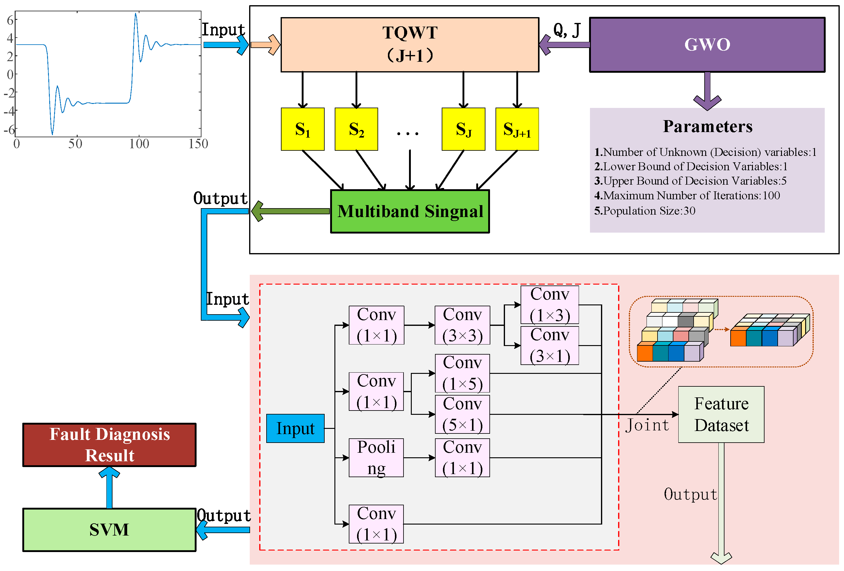
• This paper proposes integrating the improved TQWT together with the Inception model for multi-band and multiscale feature extraction to obtain the weak features of analog circuit fault signals.
• The Q-factor of the TQWT is quantized by utilizing GWO with a high capability of global optimization. The inverse TQWT is utilized along with the RMSE of the initial signal as an evaluation criterion to determine the optimal Qfactor. The optimum quality factor Q is used to decompose the signal for the TQWT and the multi-band signal is obtained via single-branch reconstruction to capture the local detail features of the signal. This optimization enables the TQWT to be more compatible with the signal characteristics and to extract more detailed features.
• The Inception model performs feature extraction on multi-band signals and multiscale feature extraction based on band differentiation, refining the features while avoiding the parameter redundancy of traditional CNNs.

2. Materials and Methods

The TQWT is an improvised version of the WT, which is more adaptable to different signals and can pick up the characteristics of the data in a more efficient way. GWO has the advantages of rapid convergence, high global search capability, and robustness, which can be used to find the optimal Q-factor of the TQWT. The Inception model can achieve multiscale feature extraction of the data based on reducing the network parameters, and it is used to derive signatures from the multi-band signals emitted from the TQWT; an SVM has good fault classification capability. Owing to the benefits of the various methods, the steps to diagnose faults on analog circuits are shown in Figure 2:

The steps of the analog circuit fault diagnosis method shown in Figure 2 are as follows:

(1)

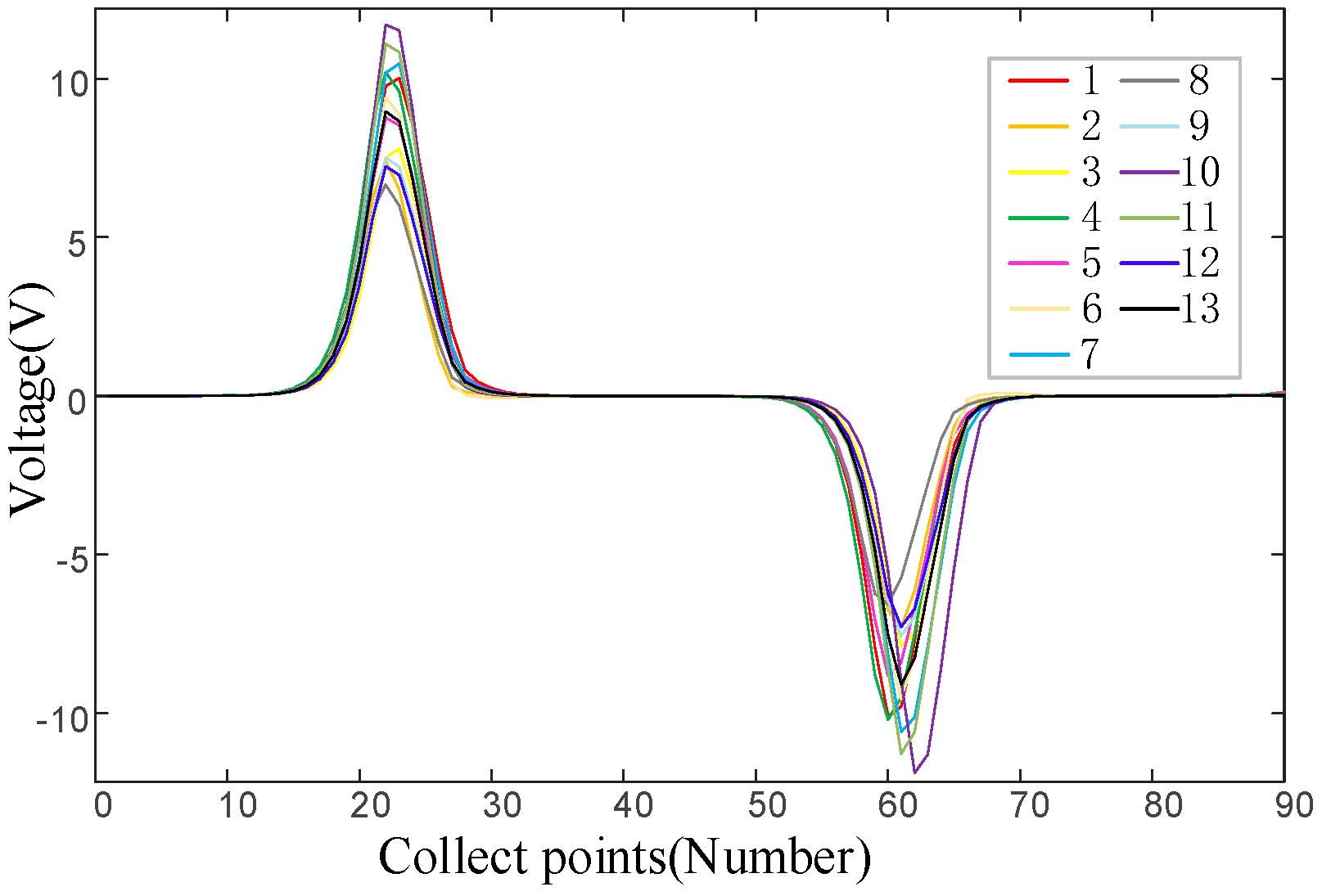
Collect the impulse response signals at the output points of the test circuits and obtain the complete initial data set via Monte Carlo analysis. The data set is divided into a training set and a test set;

(2)

Use the training set data to optimize the parameter Q of the TQWT and use the root mean square error of the decomposed and reconstructed signals as the fitness function of GWO;

(3)

Input the feature-refined data into the Inception model to train the network and initialize the network parameters;

(4)

Train the SVM model and use the RMSE of the predicted and tangible results for the fitness function;

(5)

Input the test set sample data into the trained Inception-SVM fault diagnosis model to obtain the fault diagnosis results of the test set samples.

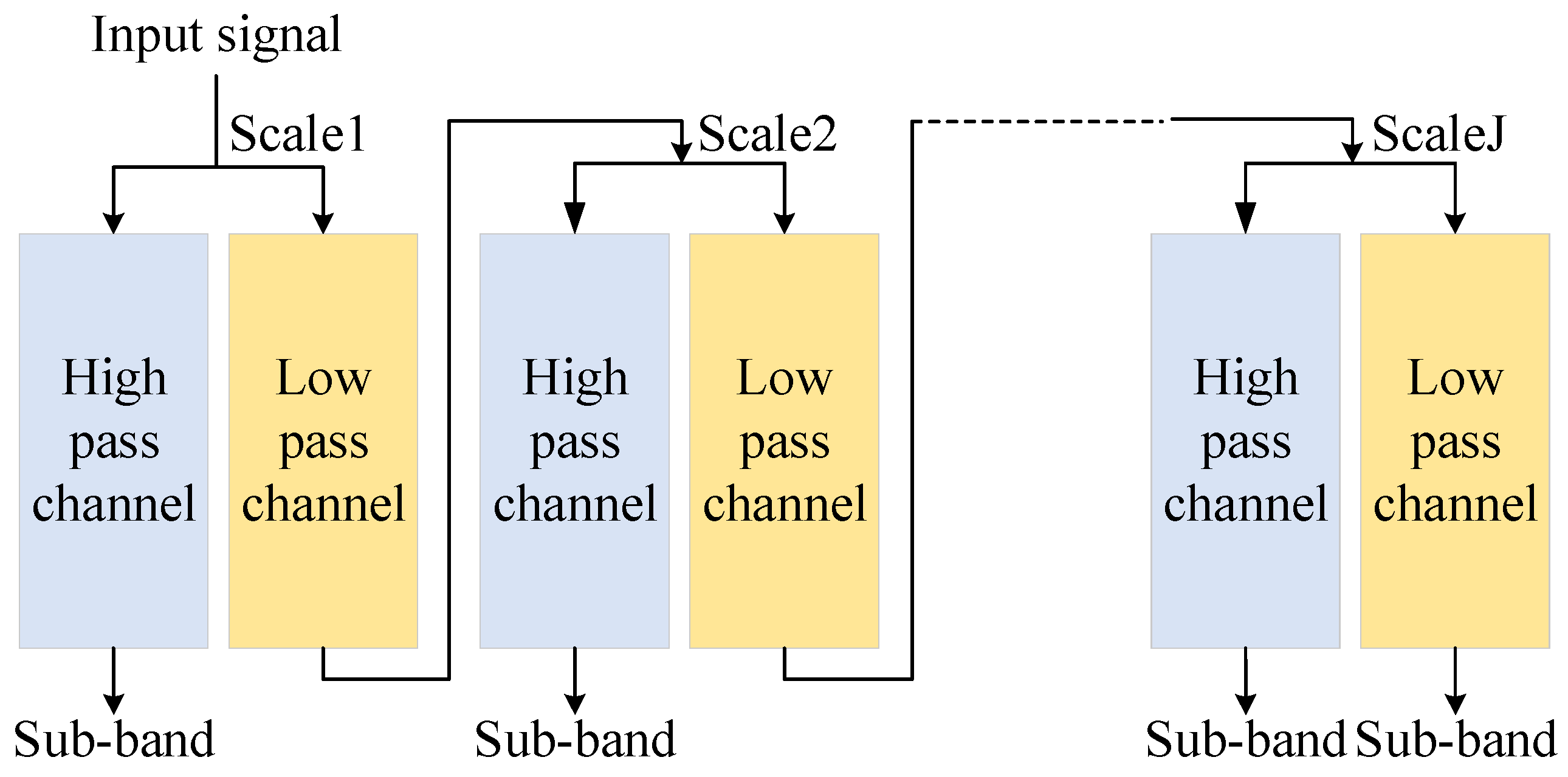
2.1. Tunable Q-Factor Wavelet Transform

In 2011, Selesnick introduced the Tunable Q-factor Wavelet transform (TQWT) [31], a discrete wavelet transform method based on wavelet basis oscillatory properties. The signal’s decomposition and reconstruction via the TQWT comprises a series of iterative two-channel filter banks. Successive executions of the high-pass and low-pass iterative decompositions in the low-pass subbands obtain the wavelet coefficient sequences for the multiscale TQWT decomposition. The J-layer decomposition of the signal using the TQWT is shown in Figure 3. Each decomposition produces one low-pass subband and one high-pass subband, and the J-layer decomposition produces a total of J + 1 subbands.

The TQWT contains three adjustable values: Q (Quality factor), r (redundancy), and J (number of levels of decomposition). Depending on the parameters, the shape and nature of the wavelet base in the TQWT are different. The functions of different parameters are as follows:

• Quality factor (Q): The proportion of the filter center frequency (f) to the bandwidth (B) used to characterize the oscillatory properties of a signal. The larger that Q is, the higher the oscillation property of the signal. The selection of the Q value determines the filter band’s selection and the signal’s filtering effect.
• Redundancy (r): the ratio of its sum of wavelet elements to the signal length, which indicates the spectral overlap between neighboring bandpass filters and is usually adopted as r = 3 [32].
• Number of decomposition levels (J): the Equation for J is shown, which shows that the TQWT decomposition consists of J layers of filters decomposed into J + 1 subbands.

$$\mathrm{J}=\lfloor \frac{\lg [\mathrm{N}/4(\mathrm{Q}+1\left)\right]}{\lg (\mathrm{Q}+1)/(\mathrm{Q}+1-2/\mathrm{r})}\rfloor$$

(1)

In Equation (1), N is the length at which the signal remains to be disassembled, $\lfloor \rfloor$ is rounded to 0.

The signal is decimated using the optimum TQWT to yield J + 1 frequency basis bands; it has J + 1 branches ranging in frequency from low to high. After sinusoidal branch reconstruction, J + 1 sets of feature data from low to high frequencies are obtained. The signature factorization and single-branch reconstitution of the TQWT is indicated for vulnerable feature estimation, which provides betterquality local time-frequency signals in subsequent element extraction and facilitates the increase in the accuracy of the fault diagnosis model.

2.2. Grey Wolf Optimization

The GWO algorithm [33] is a population-based metaheuristic algorithm inspired by the social behavior of gray wolves. The GWO algorithm includes the steps of tracking prey, encircling prey, and attacking prey. The group is separated into wolves $\mathsf{\alpha }$, wolves $\mathsf{\beta }$, wolves $\mathsf{\delta }$, and wolves $\mathsf{\omega }$. Wolves $\mathsf{\alpha }$ serve as the pack’s leader, leading wolves $\mathsf{\beta }$ and $\mathsf{\delta }$. Wolves $\mathsf{\omega }$ serve at the lowest level of the pack, with wolves $\mathsf{\alpha }$, wolves $\mathsf{\beta }$, and wolves $\mathsf{\delta }$ participating in decision-making according to the pack’s hierarchy. The harvest structure for groups of gray wolf populations is shown in Figure 4. In the figure, both A and C are random numbers in the algorithm for each type of wolfsearching process, whose formulas are described during the introduction of the algorithm. The prey is the value of the optimal Q-factor.

The basic procedures involved in finding the optimal Q-factor using GWO for the TQWT are listed below:

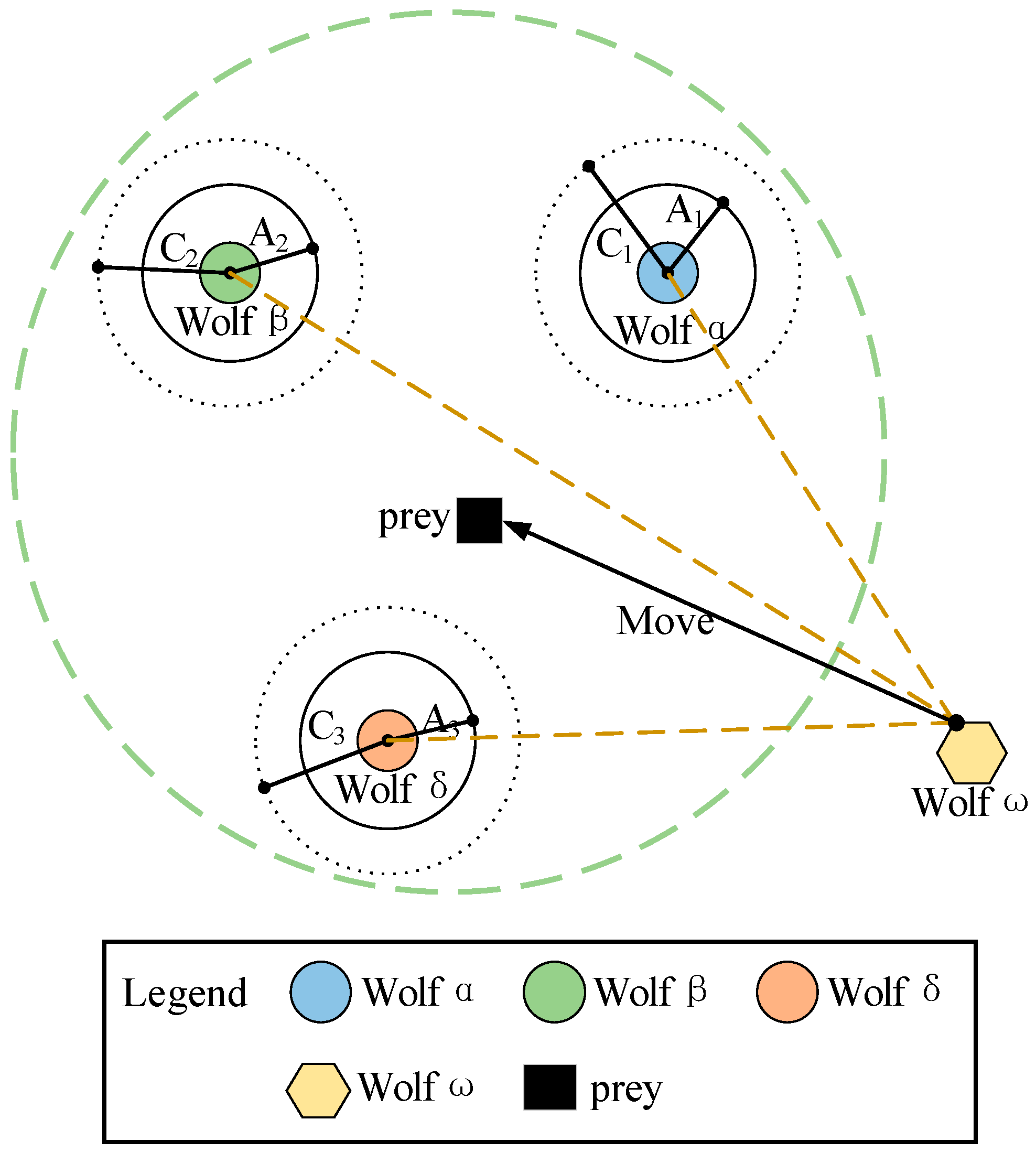
• Priming Stage: Initialize the wolves’ locations and calculate each wolf’s fitness utilizing a fitness function. The fitness function is the inverse of the Root Mean Square Error (RMSE) of the signal decomposition and reconstructed signal using the TQWT, as shown in Equation (2). The adaptation value calculated from Equation (2) was utilized to establish the hierarchy of each wolf in the colony.

  $$\mathrm{fitness}=1/\sqrt{\frac{1}{\mathrm{n}}{\displaystyle \sum _{\mathrm{i}=1}^{\mathrm{n}}[{\tilde{\mathrm{f}}}_{\mathrm{i}}-{\mathrm{f}}_{\mathrm{i}}}{]}^2}$$

  (2)
  In Equation (2), ${\mathrm{f}}_{\mathrm{i}}$ is the function value at a point, ${\tilde{\mathrm{f}}}_{\mathrm{i}}$ is the value after ${\mathrm{f}}_{\mathrm{i}}$ TQWT and the inverse TQWT, and $\mathrm{n}$ is several data points in the signaling data set.
• Envelopment phase: During the search, the gray wolf will surround the prey incrementally, which is the optimal Q. The enclosure phase is mathematically modeled as follows:

  $$\begin{array}{c}\mathrm{D}=\left|\mathrm{C}·{\mathrm{X}}_{\mathrm{P}}\left(\mathrm{t}\right)-\mathrm{X}\left(\mathrm{t}\right)\right|\\ \mathrm{X}\left(\mathrm{t}+1\right)={\mathrm{X}}_{\mathrm{p}}\left(\mathrm{t}\right)-\mathrm{A}·\mathrm{D}\\ \mathrm{A}=2\mathrm{a}·{\mathrm{r}}_1-\mathrm{a}\\ \mathrm{C}=2{\mathrm{r}}_2\end{array}$$

  (3)
  In Equation (3), $\mathrm{D}$ indicates the separation of the gray wolf from its prey, which in this experiment represents the distance between the current Q-factor position and the optimal Q-factor; $\mathrm{X}$ is the location of the gray wolf, that is, the coordinates of the most current Q-factor; $\mathrm{t}$ is the number of iterations, ${\mathrm{X}}_{\mathrm{p}}$ is the position of the optimal Q-factor, $\mathrm{A}$ and $\mathrm{C}$ are the synergy coefficients vectors, and ${\mathrm{r}}_1$, ${\mathrm{r}}_2$ are the random one-dimensional vectors in the interval between [0,1], and as the number of iterations changes from 2 to 0, the value of $\mathrm{a}$ decreases:

  $$\mathrm{a}=2-2·\mathrm{t}/\mathrm{T}$$

  (4)
  In Equation (4), $\mathrm{T}$ is the maximum number of iterations.
• Hunting stage: During this phase of hunting, wolves $\mathsf{\omega }$ renew their places following the guidance of wolves $\mathsf{\alpha },\mathsf{\beta },\mathsf{\delta }$. The numerical model of this action is:

  $$\left\{\begin{array}{l}{\mathrm{D}}_{\mathsf{\alpha }}=\left|{\mathrm{C}}_1·{\mathrm{X}}_{\mathsf{\alpha }}\left(\mathrm{t}\right)-\mathrm{X}\left(\mathrm{t}\right)\right|\\ {\mathrm{D}}_{\mathsf{\beta }}=\left|{\mathrm{C}}_2·{\mathrm{X}}_{\mathsf{\beta }}\left(\mathrm{t}\right)-\mathrm{X}\left(\mathrm{t}\right)\right|\\ {\mathrm{D}}_{\mathsf{\delta }}=\left|{\mathrm{C}}_3·{\mathrm{X}}_{\mathsf{\delta }}\left(\mathrm{t}\right)-\mathrm{X}\left(\mathrm{t}\right)\right|\end{array}\right.$$

  (5)

  $$\left\{\begin{array}{l}{\mathrm{X}}_1=\left|{\mathrm{X}}_{\mathsf{\alpha }}\left(\mathrm{t}\right)-{\mathrm{A}}_1·{\mathrm{D}}_{\mathsf{\alpha }}\right|\\ {\mathrm{X}}_2=\left|{\mathrm{X}}_{\mathsf{\beta }}\left(\mathrm{t}\right)-{\mathrm{A}}_2·{\mathrm{D}}_{\mathsf{\beta }}\right|\\ {\mathrm{X}}_3=\left|{\mathrm{X}}_{\mathsf{\delta }}\left(\mathrm{t}\right)-{\mathrm{A}}_3·{\mathrm{D}}_{\mathsf{\delta }}\right|\end{array}\right.$$

  (6)
  In the above two equations, ${\mathrm{X}}_{\mathsf{\alpha }},{\mathrm{X}}_{\mathsf{\beta }}$, and ${\mathrm{X}}_{\mathsf{\delta }}$ are the positions of wolves $\mathsf{\alpha },\mathsf{\beta }$, and $\mathsf{\delta }$, respectively.
• Termination stage: when the fitness no longer changes or the specified number of iterations is reached, the iteration stops, and the current optimal value, the best Q value obtained from the optimization search, will be output.

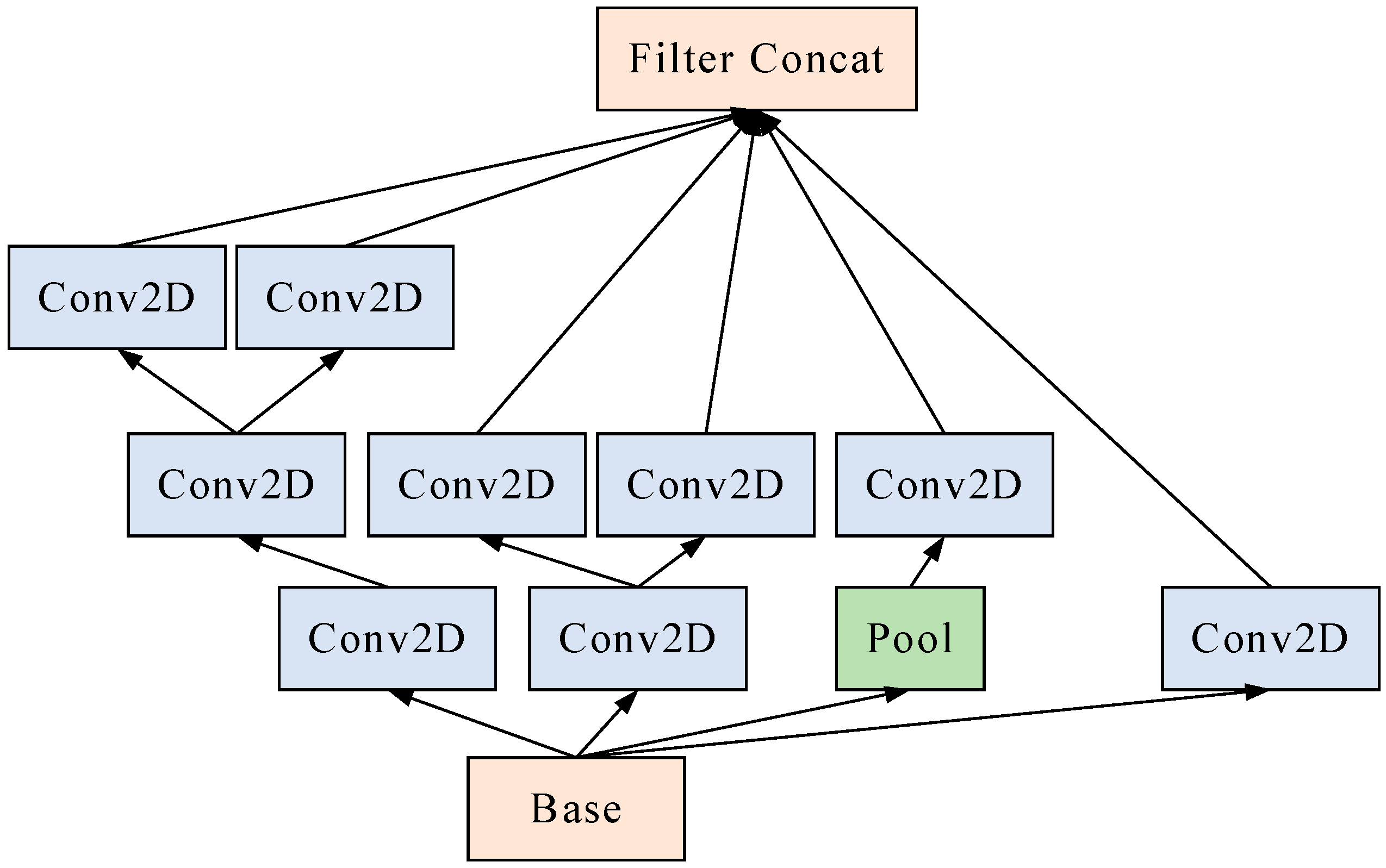
2.3. Inception Model

In 2014, Google Deep Learning proposed a convolutional neural network architecture based on the Inception model, which mainly addresses the problems of ordinary convolutional neural networks that are too computationally intensive, have many parameters, and are prone to overfitting [34]. The data input into the Inception model are divided into four paths, and the convolutional layer of each path performs different scales of data feature extraction. Then, the data are spliced in the concatenate layer and output. The model replaces large convolutional kernels with stacked small convolutional kernels, which reduces the number of network parameters. The Inception model has gone through a series of improvements and upgrades since it was proposed, and this study is based on the Inception V3 model, which is used to carry out multiscale feature extraction on the local time-frequency signals output from the TQWT to complete the whole feature extraction step. Its structure is shown in Figure 5. In the figure, Conv2D is the 2D convolutional layer, and Pool is the pooling layer.

The model was chosen based on the following demands:

• Obtaining multiscale features: the amount of computation in different branches of the Inception model can be allocated different computational resources by adjusting the parameters to obtain the best multiscale features.
• Reduction in network parameters: decomposed convolution is used, where a large convolutional kernel is decomposed into multiple smaller convolutional kernels, thus reducing the number of parameters and the amount of calculations.
• Improved network efficiency: a 3 × 3 convolutional kernel is introduced, which reduces the parameter count and increases the effectiveness and performance in the network compared to the previous 5 × 5 convolutional kernel.

2.4. SVM

An SVM [35] is one of the mechanical learned encoding algorithms based on which the statistical learning theorem is used for classification and regression. The principle efficiently classifies samples by selecting sample points as support vectors and finding the optimal hyperplanes in the feature space to maximize the distance between different samples. When dealing with nonlinear problems, the nuclear constructor can map the data to a high-dimensional space and use an optimal hyperplane to complete the classification. When dealing with multi-classification problems, the objective function can be modified to combine the parameter-solving problems of multiple classification surfaces with each other and convert them into the optimization of one problem. A multi-classifier can also be constructed by combining multiple binary classifiers, commonly known as one-to-many methods, one-to-one methods, and so on [36,37]. The use of an SVM for the classification of the feature data of analog circuits has the characteristics of good general performance and adaptability. It is the most common and effective Radial Basis Function (RBF) kernel for performing fault classification.

$$\mathrm{K}\left({\mathrm{x}}_{\mathrm{i}},{\mathrm{x}}_{\mathrm{j}}\right)=\exp \left(-\mathrm{g}{‖{\mathrm{x}}_{\mathrm{i}}-{\mathrm{x}}_{\mathrm{j}}‖}^2\right)$$

(7)

In Equation (7), ${‖{\mathrm{x}}_{\mathrm{i}}-{\mathrm{x}}_{\mathrm{j}}‖}^2$ is the Euclidean distance between ${\mathrm{x}}_{\mathrm{i}}$ and ${\mathrm{x}}_{\mathrm{j}}$. $\mathrm{g}$ is given by $\mathrm{g}=\frac{1}{2{\mathsf{\sigma }}^2}$, where $\mathsf{\sigma }$ is a freedom parameter.

3. Simulation Experiments and Discussion

The simulation experiments based on a Sallen–Key bandpass filter circuit and a four-op-amp dual second-order high-pass filter circuit demonstrate the validity of the suggested soft fault diagnosis approaches for analog circuits. This section describes how to perform the simulation experiments and analyze the results.

The experiments were carried out on a computer with a memory of 16 GB. The data decomposition, reconstruction, and singlebranch reconstruction were performed using C++ programming on the Matlab platform. The rest of the steps used Python programming in a TensorFlow environment. The software used for the simulation of circuits was Multisim 14.0.

3.1. Verify Circuit and Fault Settings

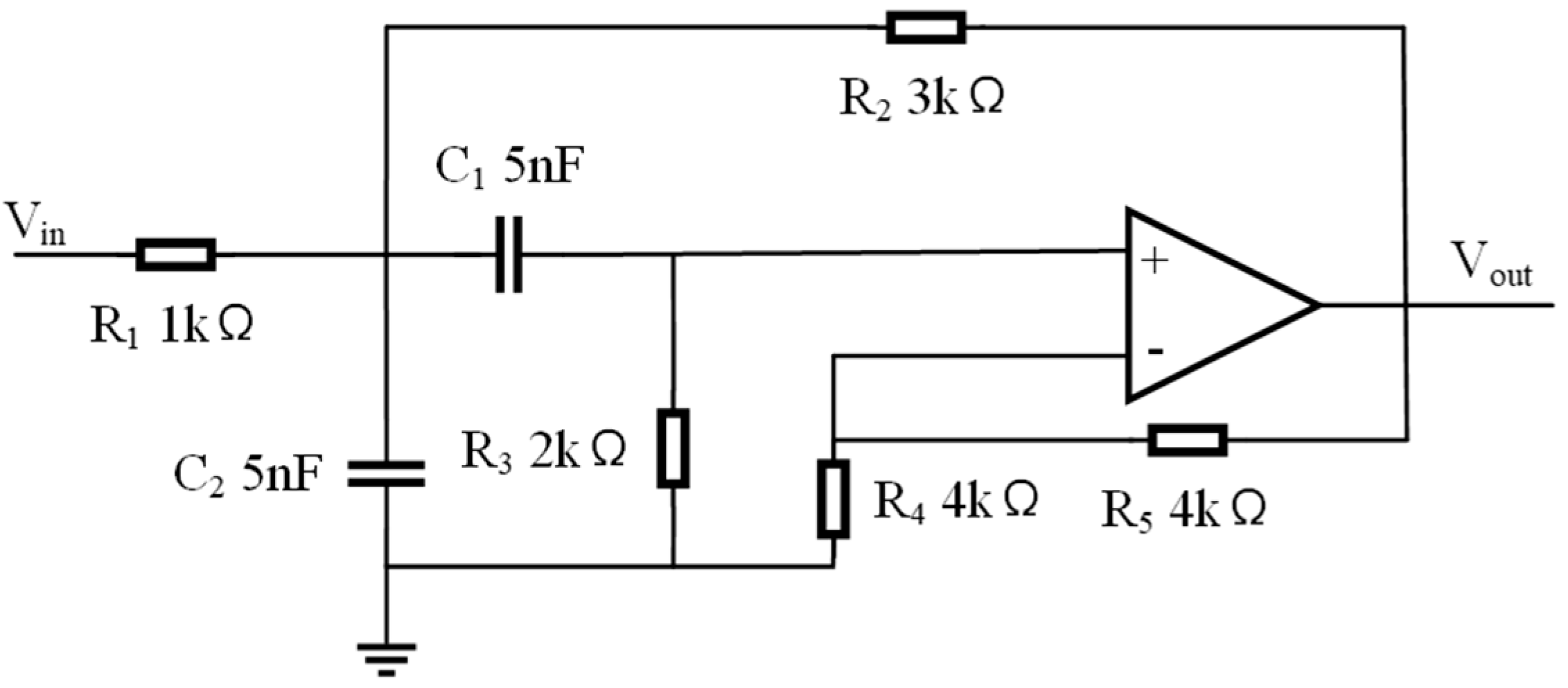
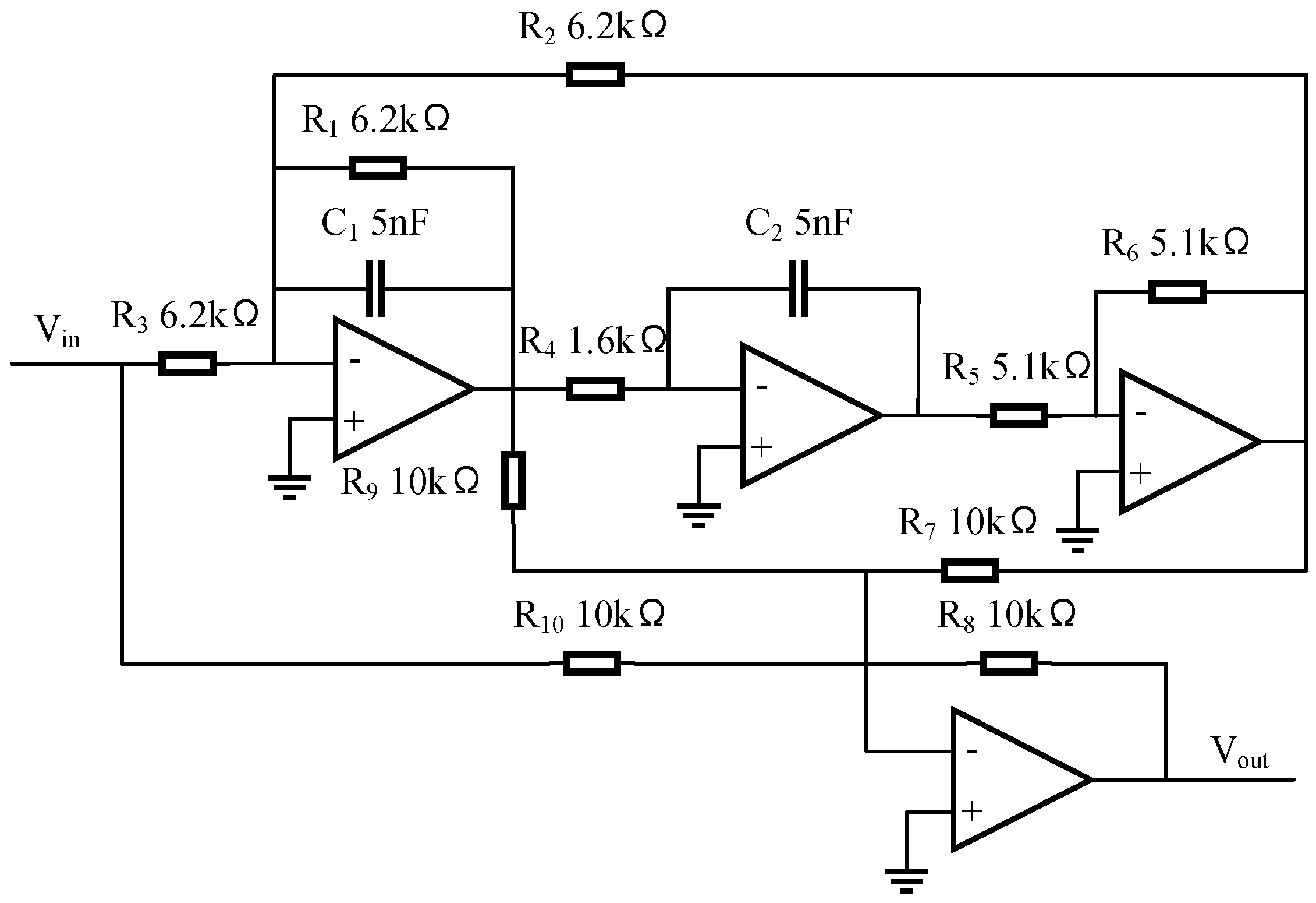
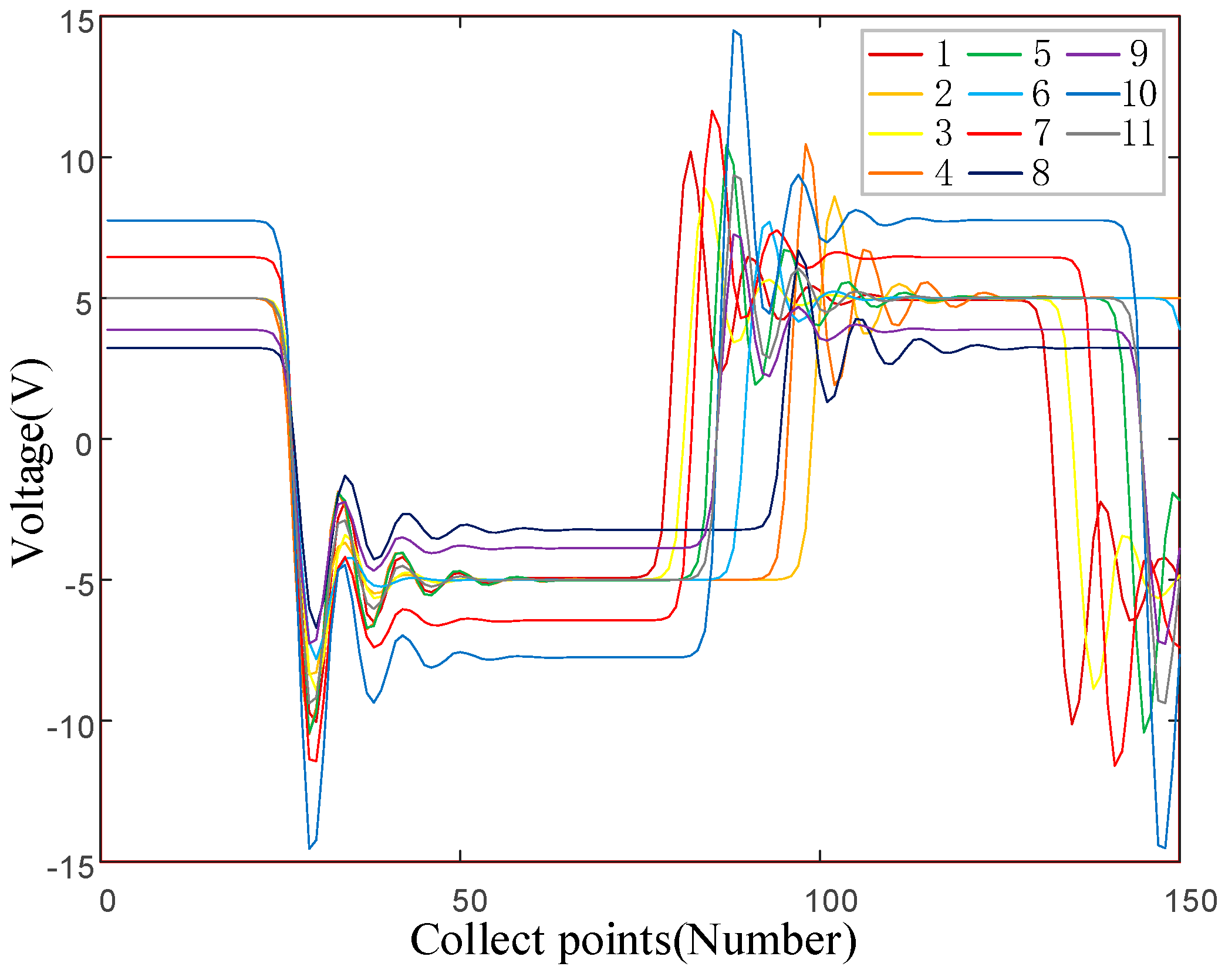
• Case1: Sallen–Key bandpass filter circuit

Circuit and fault settings: The Sallen-Key bandpass filter circuit is shown in Figure 6. According to the sensitivity analysis of the circuit, C₁, C₂, R₂, R₃, R₄, and R₅ were selected as the test components, in which the tolerance range of resistors and capacitors was set to 20%, and then there were 13 failure modes in the circuit, which were as follows: C₁↑, C₁↓, C₂↑, C₂↓, R₂↑, R₂↓. R₃↑, R₃↓, R₄↑, R₄↓, R₅↑, R₅↓, and NF (no fault).↑ and↓ refer to higher or lower than the component no fault critical value. The failure modes and component failure range of this circuit are shown in

Table 1. Fault types and corresponding values of Sallen–Key bandpass filter circuits.

Fault Type	Fault Label	Normal Value	Range of Fault
C1↑	1	5 nF	[6 nF, 7.5 nF]
C1↓	2	5 nF	[2.5 nF, 4 nF]
C2↑	3	5 nF	[6 nF, 7.5 nF]
C2↓	4	5 nF	[2.5 nF, 4 nF]
R2↑	5	3 KΩ	[3.6 kΩ, 4.5 kΩ]
R2↓	6	3 KΩ	[1.5 kΩ, 2.4 kΩ]
R3↑	7	2 KΩ	[2.4 kΩ, 3 kΩ]
R3↓	8	2 KΩ	[1 kΩ, 1.6 kΩ]
R4↑	9	4 KΩ	[4.8 kΩ, 6 kΩ]
R↓	10	4 KΩ	[2 kΩ, 3.2 kΩ]
R5↑	11	4 KΩ	[4.8 kΩ, 6 kΩ]
R5↓	12	4 KΩ	[2 kΩ, 3.2 kΩ]
NF	13	/	/

.

The experiment selected the 1 ms period and 5 V amplitude pulse signal as the excitation signal, and the duty cycle of the excitation signal was 50%. It also used Multisim 14.0 to simulate the circuit. The exit point of the circuit was the point at which the circuit signals were captured. By conducting Monte Carlo analysis, 200 signals were generated for each fault mode, and 2600 sets of samples were obtained; 70% of the samples served as the training set and 30% served as the test set to construct the training and test sets of Case1. The original signals of different fault types of Case1 and their visualization of the features after feature extraction are shown in Figure 7 and Figure 8, respectively.

• Four-op-amp biquad high-pass filter circuit

Circuit and fault settings: The four op-amp dual second-order high-pass filter circuit is shown in Figure 9. According to the sensitivity analysis of the circuit, C₁, C₂, R₁, R₂, and R₃ were the test components, where the resistance and capacitance of the tolerance range were set to 20%. There were 11 failure modes in the circuit: C₁↑, C₁↓, C₂↑, C₂↓, R₁↑, R₁↓, R₂↑, R₂↓, R₃↑, R₃↓, and NF (No Fault). The failure modes and component failure range for this circuit are shown in

Table 2. Fault types and corresponding values of the four-op-amp biquad high-pass filter circuit.

Fault Type	Fault Label	Normal Value	Range of Fault
C1↑	1	5 nF	[6 nF, 7.5 nF]
C1↓	2	5 nF	[2.5 nF, 4 nF]
C2↑	3	5 nF	[6 nF, 7.5 nF]
C2↓	4	5 nF	[2.5 nF, 4 nF]
R1↑	5	6.2 KΩ	[7.44 kΩ, 9.3 kΩ]
R1↓	6	6.2 KΩ	[3.1 kΩ, 4.96 kΩ]
R2↑	7	6.2 KΩ	[7.44 kΩ, 9.3 kΩ]
R2↓	8	6.2 KΩ	[3.1 kΩ, 4.96 kΩ]
R3↑	9	6.2 KΩ	[7.44 kΩ, 9.3 kΩ]
R3↓	10	6.2 KΩ	[3.1 kΩ, 4.96 kΩ]
NF	13	/	/

.

The input signal for Case2 was still the pulse signal with a period of 1 ms and an amplitude of 5 V with a 50% duty cycle as the excitation signal. The circuit was simulated using Multisim 14.0, and the output point of the circuit was the point where the signal of the circuit was captured (that is, V_out in the circuit). Through Monte Carlo analysis, 200 signals were generated for each fault mode, and 2200 sets of samples were obtained for the 11 fault types to construct the data set for Case2. The data set was divided into 70% training sets and 30% test sets. The original signals of different fault types of Case2 and their visualized features after feature extraction are shown in Figure 10 and Figure 11, respectively.

3.2. Parameter Selection and Related Experiments

The Qfactor of the TQWT is usually set at 3. However, owing to the variability of the data, the Qfactor of the TQWT significantly impacts the experimental results, so GWO was used to optimize it. The optimized results are compared with the experimental results at Q = 3, and the comparison results are shown in

Table 3. Circuit failure accuracy for different Q-factors.

Circuits	Q = 3	Search for Superior Q-Value
Case1	95.46%	100%
Case2	96.59%	99.09%

:

The Q-factor was most applicable to Case1 and Case2 and could be optimized via GWO, whereby the number of decomposition layers J was computed, and the Q-factors obtained via Case1 and Case2 optimization were 1.34 and 3.45, respectively. The network parameters of the Inception model are shown in

Table 4. Parameters of the Inception model.

Layer	Parameters
Conv2D	filters = 128, Strides = (2,2), Kernel_size = (1,1)
Conv2D	filters = 128, Strides = (2,2), Kernel_size = (3,3)
Conv2D	filters = 64, Strides = (1,1), Kernel_size = (1,3)
Conv2D	filters = 64, Strides = (1,1), Kernel_size = (3,1)
Conv2D	filters = 256, Strides = (1,1), Kernel_size = (1,1)
Conv2D	filters = 64, Strides = (1,1), Kernel_size = (1,5)
Conv2D	filters = 64, Strides = (1,1), Kernel_size = (5,1)
MaxPooling2D	pool_size = (2,2), Strides = (2,2)
Conv2D	filters = 64, Strides = (1,1), Kernel_size = (1,1)
Conv2D	filters = 64, Strides = (1,1), Kernel_size = (1,1)

:

3.3. Results of the Experiment

An experiment with 50 independent repetitions was conducted on the data of Case1 and Case2. The accuracy rate of Case1 was 100% and that of Case2 was 99.09%. The obfuscation matrix of its fault diagnosis is presented in Figure 12. The figure shows that for Case1, the predicted labels for its fault classification are the actual labels. For Case2, the faults with labels 4 and 5 were prone to confusion, but overall, the accuracy of fault diagnosis could be up to 99.90%. Therefore, a fault diagnosis method for analog circuits based on the improved TQWT and Inception model can achieve the fault diagnosis of analog circuits.

The approach suggested herein was compared with the classical fault diagnosis methods, as shown in

Table 5. Comparison of the experimental results for the different methods.

Method	Case1	Case2
This paper	100%	99.09%
TQWT-CNN [38]	99.10%	98.96%
FRFT-CNN [39]	98.46%	95.15%
GMKL-SVM [40]	100%	97.58%
IEEMD-SVM [14]	98.72%	96.36%
Improved WT-MKELM [21]	100%	98.75%

. The TQWT-CNN [38] model uses an improved TQWT and CNN-LSTM network to conduct characteristic extraction and uses a CNN network to complete the fault diagnosis; FRFT-CNN [39] uses the fractional Fourier transform to transform the signal’s statistical characteristic features as the fault features, and then uses KPCA to downscale the features to obtain the optimal features, and finally uses a Convolutional Neural Network for fault classification. GMKL-SVM [40] extracts the wavelet coefficient energy of the signal as the features and then uses the Particle Swarm Optimization (PSO) optimized Generalized Multi Kernel Learning-Support Vector Machine (GMKL-SVM) for fault classification. The IEEMD-SVM [14] performs the empirical pattern decomposition of the signal, extracts the independent IMF as the feature data, and uses an SVM for fault classification. The improved WT-MKELM [21] considers the features of the improved WT as the best features and uses an optimized MKELM with PSO to identify different faults. Based on the results in the table, it can be concluded that a fault diagnosis method for analog circuits based on the improved TQWT and Inception model proposed in this paper is superior to the classical fault diagnosis methods. Using the GWO-optimized TQWT for the time-frequency decomposition of signals and the Inception model for multiscale feature extraction can effectively obtain the feature information of signals and improve the fault diagnosis accuracy of analog circuits.

4. Conclusions

Given the complexity of the fault identification in analog circuits, a new approach to fault diagnosis is introduced for fault signature acquisition and classification. When performing feature extraction, the TQWT is used for the multi-band decomposition of the data simultaneously. Since the parameter Q of the TQWT has a large influence on the wavelet basis, GWO is utilized to optimize the Q. After the TQWT, the Inception model is used for multiscale feature extraction to obtain the signal features adequately. A Support Vector Machine with a better classification effect is used for fault classification. The method is validated using the Sallen–Key bandpass filter circuit and the four-op-amp biquad high-pass filter circuit, and the fault diagnosis accuracies of the two circuits are 100% and 99.09%, respectively. The empirical evidence indicated that the presented approach can be used for the fault diagnosis of analog circuits, which is conducive to enhancing the stability and security of power supply systems. Forthcoming work will focus on applying the method in complex real circuits.

References

1. Huang, J.; Zhang, X.; Shuai, Z.; Zhang, X.; Wang, P.; Koh, L.H.; Xiao, J.; Tong, X. Robust Circuit Parameters Design for the CLLC-Type DC Transformer in the Hybrid AC–DC Microgrid. IEEE Trans. Ind. Electron. 2019, 66, 1906–1918. [Google Scholar] [CrossRef]
2. Zhang, C.; Zha, D.; Wang, L.; Mu, N. A Novel Analog Circuit Soft Fault Diagnosis Method Based on Convolutional Neural Network and Backward Difference. Symmetry 2021, 13, 1096. [Google Scholar] [CrossRef]
3. Tadeusiewicz, M.; Halgas, S.A. Method for Local Parametric Fault Diagnosis of a Broad Class of Analog Integrated Circuits. IEEE Trans. Instrum. Meas. 2018, 67, 328–337. [Google Scholar] [CrossRef]
4. Wang, N. The analysis of electronic circuit fault diagnosis based on neural network data fusion algorithm. Symmetry 2020, 12, 458. [Google Scholar] [CrossRef]
5. Jia, R.; Wang, J.; Zhou, J. Fault diagnosis of industrial process based on the optimal parametric t-distributed stochastic neighbor embedding. Sci. China Inf. Sci. 2021, 64, 229–231. [Google Scholar] [CrossRef]
6. Marin, C.V.; Constantinescu, F.; Nitescu, M. A dictionary approach to fault diagnosis of analog circuits. In IEEE Africon’11; IEEE: Victoria Falls, Zambia, 2011; pp. 13–15. [Google Scholar] [CrossRef]
7. Lalami, A.; Wamkeue, R. Synchronous generator off-line diagnosis approach including fault detection and estimation of failures on machine parameters. Electr. Power Compon. Syst. 2013, 41, 1501–1517. [Google Scholar] [CrossRef]
8. Contu, S.; Fanni, A.; Marchesi, M.; Montisci, A.; Serri, A. Wavelet analysis for diagnostic problems. In Proceedings of the 8th Mediterranean Electrotechnical Conference, Bari, Italy, 16 May 1996. [Google Scholar] [CrossRef]
9. Hong, S.; Tang, J.; Chen, X. Analog circuit fault diagnosis combing wavelet packet with higher order statistics. In Proceedings of the 2010 2nd International Conference on Signal Processing Systems, Dalian, China, 5–7 July 2010. [Google Scholar] [CrossRef]
10. He, Y.G.; Tan, Y.H.; Sun, Y. A neural network approach for fault diagnosis of large-scale analogue circuits. IEEE Int. Symp. Circuits Syst. 2002, 4, 151. [Google Scholar] [CrossRef]
11. Yang, Y.; Wang, L.; Nie, X.; Wang, Y. Incipient fault diagnosis of analog circuits based on wavelet transform and improved deep convolutional neural network. IEICE Electron. Express 2021, 18, 20210174. [Google Scholar] [CrossRef]
12. Wang, G.; Feng, D.; Tang, W. Electrical impedance tomography based on grey wolf optimized radial basis function neural network. Micromachines 2022, 13, 1120. [Google Scholar] [CrossRef]
13. Gan, X.S.; Cui, H.L.; Wu, Y.R. WNN Model Based on Particle Swarm Optimization for Fault Diagnosis in Analog Circuit. Appl. Mech. Mater. 2013, 427–429, 1048–1051. [Google Scholar] [CrossRef]
14. Shokrolahi, S.M.; Kazempour, A.T.N. A novel approach for fault detection of analog circuit by using improved EEMD. Analog. Integrated. Circuits Signal Process. 2019, 98, 527–534. [Google Scholar] [CrossRef]
15. Xiong, J.; Tian, S.; Yang, C. Fault Diagnosis for Analog Circuits by Using EEMD, Relative Entropy, and ELM. Comput. Intell. Neurosci. 2016, 2016, 7657054. [Google Scholar] [CrossRef]
16. Yang, H.; Meng, C.; Wang, C. Data-driven Feature Extraction for Analog Circuit Fault Diagnosis Using 1-D Convolutional Neural Network. IEEE Access 2020, 8, 18305–18315. [Google Scholar] [CrossRef]
17. Gilles, J. Empirical Wavelet Transform. Signal Process. IEEE Trans. 2013, 61, 3999–4010. [Google Scholar] [CrossRef]
18. Bi, X.; Cao, S.; Zhang, D. Diesel Engine Valve Clearance Fault Diagnosis Based on Improved Variational Mode Decomposition and Bispectrum. Energies 2019, 12, 661. [Google Scholar] [CrossRef]
19. Zhang, C.; He, Y.; Yuan, L.; Xiang, S. Analog Circuit Incipient Fault Diagnosis Method Using DBN Based Features Extraction. IEEE Access 2018, 6, 23053–23064. [Google Scholar] [CrossRef]
20. Gan, X.S.; Qu, H. Research on ELM soft fault diagnosis of analog circuit based on KSLPP feature extraction. IEEE Access 2019, 7, 92517–92527. [Google Scholar] [CrossRef]
21. Zhang, C.; He, Y.; Yang, T.; Zhang, B.; Wu, J. An Analog Circuit Fault Diagnosis Approach Based on Improved Wavelet Transform and MKELM. Circuits Syst. Signal Process. 2022, 1, 1255–1286. [Google Scholar] [CrossRef]
22. Liu, Z.; Lin, Z.; Wang, C. Kent-PSO optimized ELM fault diagnosis model in analog circuits. J. Phys. Conf. Ser. 2021, 1871, 012053. [Google Scholar] [CrossRef]
23. Yu, W.X.; Sui, Y.; Wang, J. The Faults Diagnostic Analysis for Analog Circuit Based on FA-TM-ELM. J. Electron. Test. 2016, 32, 459–465. [Google Scholar] [CrossRef]
24. Bhuvaneshwari, P.; Rao, A.N.; Robinson, Y.H. Spam review detection using self attention based CNN and bi-directional LSTM. Multimed. Tools Appl. 2021, 80, 18107–18124. [Google Scholar] [CrossRef]
25. Zhao, G.Q.; Liu, X.Y.; Zhang, B.; Liu, Y.; Niu, G.; Hu, C. A novel approach for analog circuit fault diagnosis based on Deep Belief Network. Measurement 2018, 121, 170–178. [Google Scholar] [CrossRef]
26. Gao, T.; Yang, J.; Jiang, S.; Yan, G. A Novel Fault Diagnosis Method for Analog Circuits Based on Conditional Variational Neural Networks. Circuits Syst. Signal Process. 2020, 40, 2609–2633. [Google Scholar] [CrossRef]
27. Liang, H.; Zhu, Y.; Zhang, D.; Chang, L.; Lu, Y.; Zhao, X.; Guo, Y. Analog Circuit Fault Diagnosis Based on Support Vector Machine Classifier and Fuzzy Feature Selection. Electronics 2021, 10, 1496. [Google Scholar] [CrossRef]
28. Yuan, X.; Liu, Z.; Miao, Z.; Zhao, Z.; Zhou, F.; Song, Y. Fault Diagnosis of Analog Circuits Based on IH-PSO Optimized Support Vector Machine. IEEE Access 2019, 7, 137945–137958. [Google Scholar] [CrossRef]
29. Gao, T.; Yang, J.; Jiang, S. A Novel Incipient Fault Diagnosis Method for Analog Circuits Based on GMKL-SVM and Wavelet Fusion Features. IEEE Trans. Instrum. Meas. 2020, 70, 1–15. [Google Scholar] [CrossRef]
30. Lin, L. Research on analog circuit fault diagnosis method. Mod. Electron. Tech. 2017, 40, 183–186. [Google Scholar] [CrossRef]
31. Selesnick, I.W. Wavelet Transform With Tunable Q-Factor. IEEE Trans. Signal Process. 2011, 59, 3560–3575. [Google Scholar] [CrossRef]
32. Hu, Y.T.; Zhou, Q.; Gao, J.; Li, J.; Xu, Y. Compound fault diagnosis of rolling bearings based on improved tunable Q-factor wavelet transform. Meas. Sci. Technol. 2021, 32, 105018. [Google Scholar] [CrossRef]
33. Pramanik, R.; Pramanik, P.; Sarkar, R. Breast cancer detection in thermograms using a hybrid of GA and GWO based deep feature selection method. Expert Syst. Appl. 2023, 219, 119643. [Google Scholar] [CrossRef]
34. Yang, G.; Guan, K.; Yang, J.; Zou, L.; Yang, X. Penetration State Identification of Aluminum Alloy Cold Metal Transfer Based on Arc Sound Signals Using Multi-Spectrogram Fusion Inception Convolutional Neural Network. Electronics 2023, 12, 4910. [Google Scholar] [CrossRef]
35. Abdelwanis, M.I.; El-Sousy, F.F.M.; Ali, M.M. A Fuzzy-Based Proportional–Integral–Derivative with Space-Vector Control and Direct Thrust Control for a Linear Induction Motor. Electronics 2023, 12, 4955. [Google Scholar] [CrossRef]
36. Zhu, J.; Ma, C.; Zhang, Y.; Huang, H.; Kong, D.; Ni, W. Multi-Label Diagnosis of Arrhythmias Based on a Modified Two-Category Cross-Entropy Loss Function. Electronics 2023, 12, 4976. [Google Scholar] [CrossRef]
37. Wang, X.; Ling, Y.; Ling, X.; Li, X.; Li, Z.; Hu, K.; Dai, M.; Zhu, J.; Du, Y.; Yang, Q. A particle swarm algorithm optimization-based SVM–KNN algorithm for epileptic EEG recognition. Int. J. Intell. Syst. 2022, 37, 11233–11249. [Google Scholar] [CrossRef]
38. Yuan, X.; Sheng, Y.; Zhuang, X.; Yin, J.; Yang, S. A novel fault diagnosis method for second-order bandpass filter circuit based on TQWT-CNN. PLoS ONE 2024, 19, e0291660. [Google Scholar] [CrossRef] [PubMed]
39. Song, P.; He, Y.; Cui, W.J. Statistical property feature extraction based on FRFT for fault diagnosis of analog circuits. Analog. Integr. Circ. Sig Process 2016, 87, 427–436. [Google Scholar] [CrossRef]
40. Zhang, C.; He, Y.; Yuan, L.; He, W.; Xiang, S.; Li, Z.G. A Novel Approach for Diagnosis of Analog Circuit Fault by Using GMKL-SVM and PSO. J. Electron. Test. 2016, 32, 531–540. [Google Scholar] [CrossRef]
Figure 1. Fault classification of analog circuits.
Symmetry 16 00720 g001
Figure 2. The method proposed in this paper.
Symmetry 16 00720 g002
Figure 3. The process of TQWT signal decomposition.
Symmetry 16 00720 g003
Figure 4. Structural diagram of gray wolf hunting.
Symmetry 16 00720 g004
Figure 5. Architecture diagram of the Inception model.
Symmetry 16 00720 g005
Figure 6. Sallen–Key bandpass filter circuit.
Symmetry 16 00720 g006
Figure 7. Sallen–Key bandpass filtering circuits time-series signals for different fault types.
Symmetry 16 00720 g007
Figure 8. Feature visualization of the Sallen–Key bandpass filter circuit training set data after the Inception model.
Symmetry 16 00720 g008
Figure 9. Four-op-amp biquad high-pass filter circuit.
Symmetry 16 00720 g009
Figure 10. Four-op-amp biquad high-pass filter circuit for different fault types of timeseries signals.
Symmetry 16 00720 g010
Figure 11. After feature visualization via the Inception model, the training set data of the four-op-amp biquad high-pass filter circuit.
Symmetry 16 00720 g011
Figure 12. Confusion matrix for the prediction results: (a) Confusion matrix of Case1 prediction results; (b) Confusion matrix of Case2 prediction results.
Symmetry 16 00720 g012