
Numerical Solution of the Linear Fractional Delay Differential Equation Using Gauss–Hermite Quadrature


Abstract
:1. Introduction
- The Laplace transform converts the complex FDDE into a simpler algebraic equation in the Laplace domain. This transformation significantly reduces the challenge of solving differential equations with fractional derivatives and delays, which leads to a more regulated and efficient procedure.
- The Laplace transform effectively incorporates the initial conditions into the transformed equation. This feature is particularly beneficial for FDDEs because it makes it possible to provide initial states easily without the need for more intricate manipulations.
- The Laplace transform method is applicable to a large class of FDDEs with different kinds of fractional derivative and delay terms. This adaptability makes it a powerful tool in a variety of fields such as applied mathematics, physics, engineering, and control theory.
2. Preliminaries
3. Existence
4. Stability
5. Numerical Method
Gauss–Hermite Quadrature Rule
6. Application
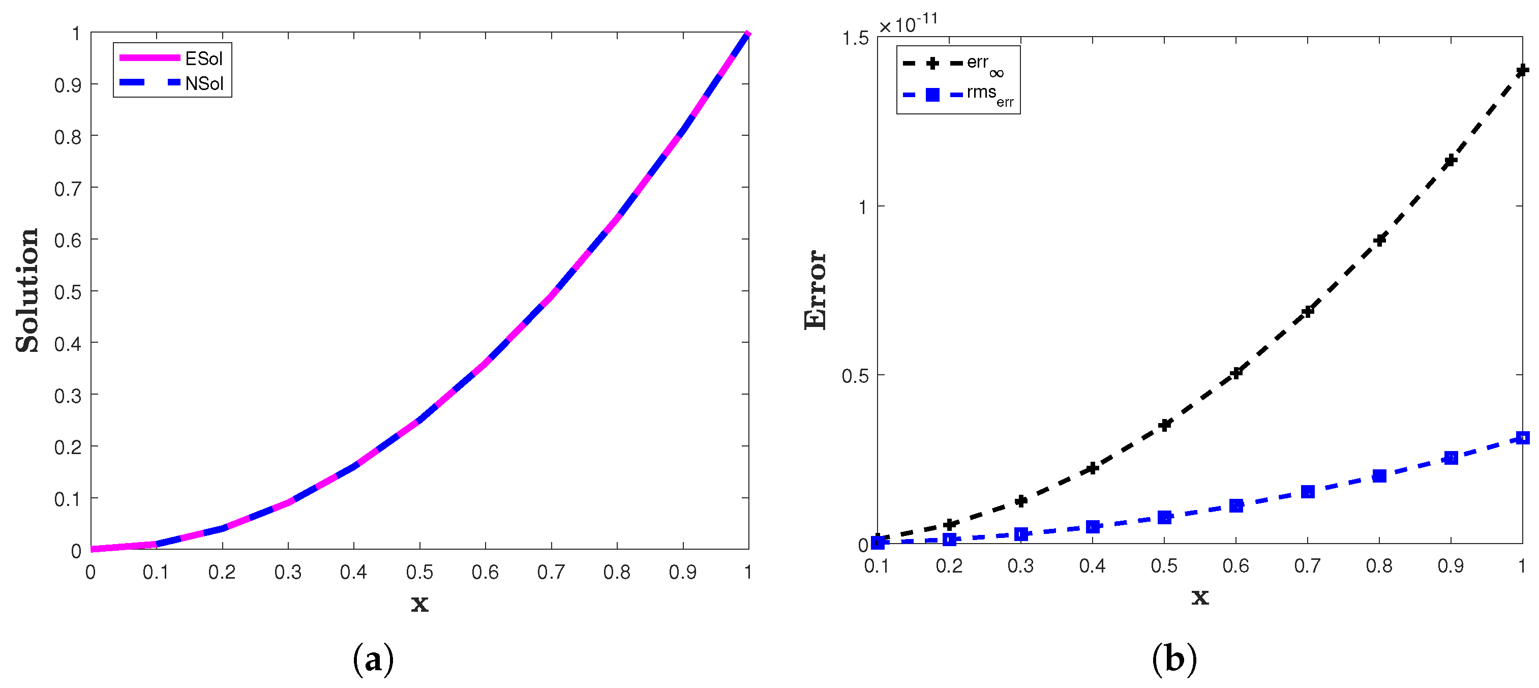
6.1. Example 1
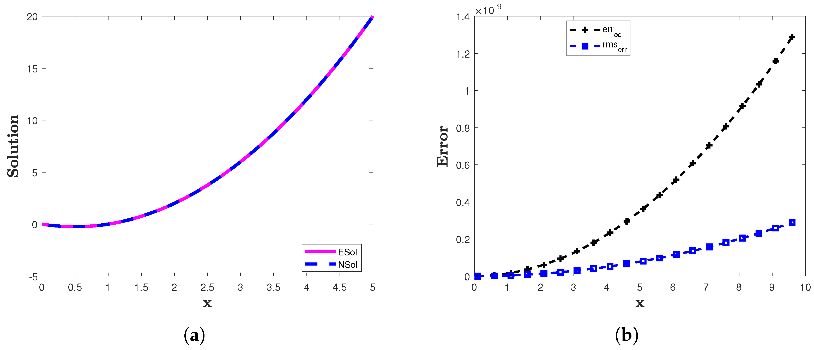
6.2. Example 2
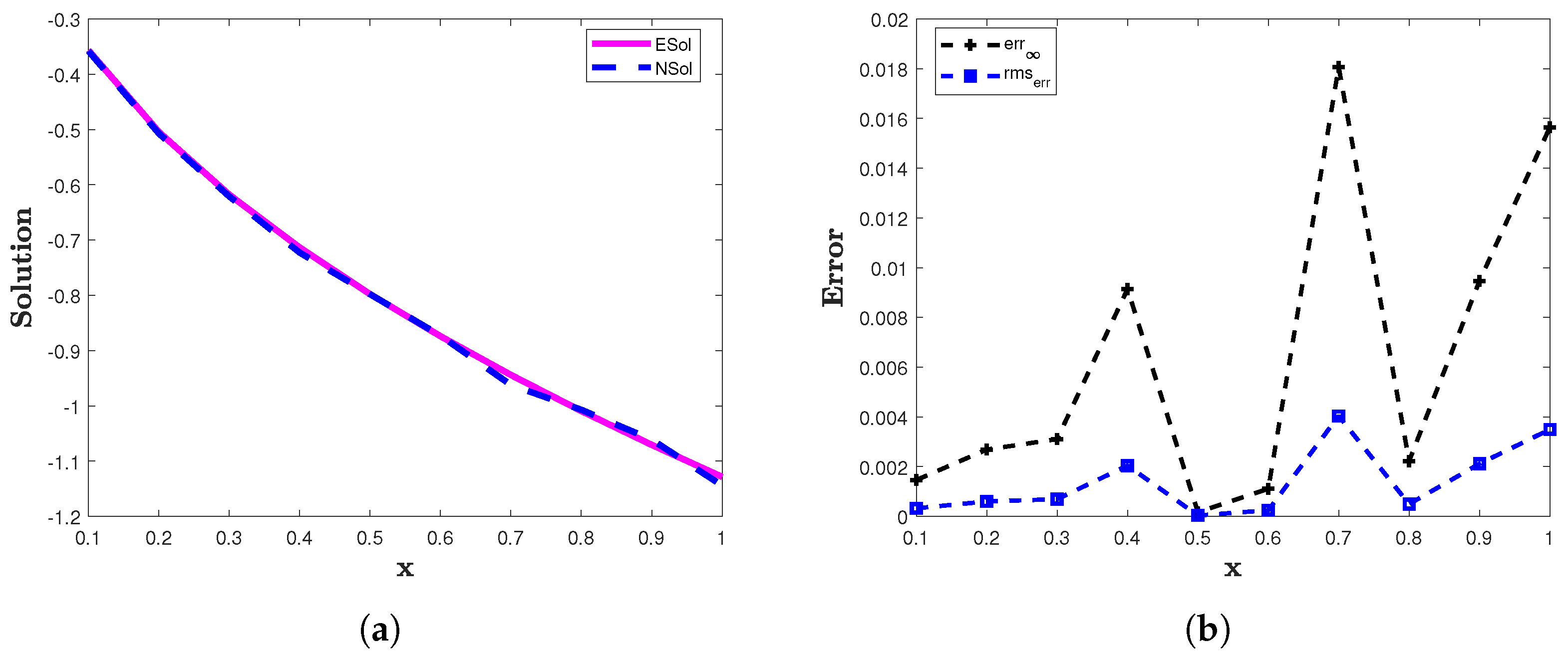
6.3. Example 3
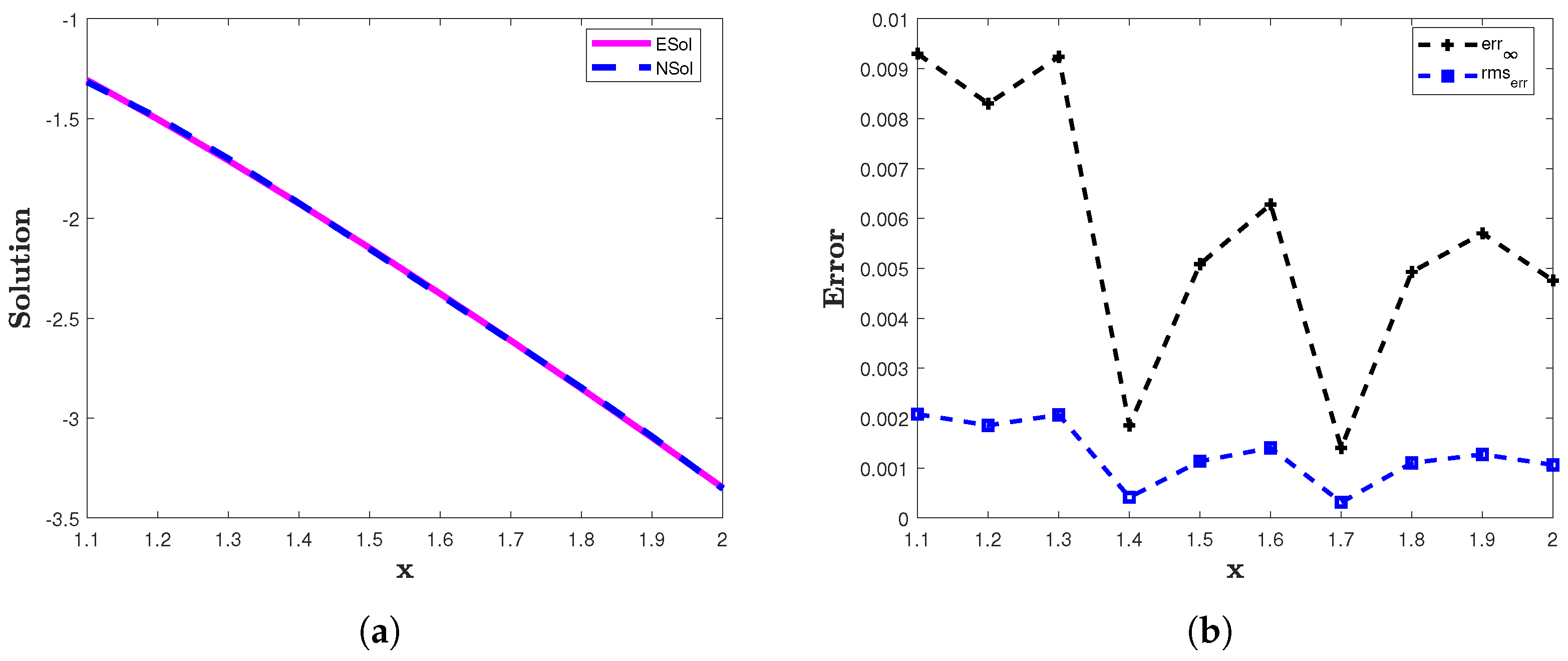
6.4. Example 4
7. Conclusions
- The error is very small in our approximations.
- The proposed method produces accurate results in a very short computation time.
- The results demonstrate that the proposed method can solve FDDEs efficiently.
Author Contributions
Funding
Data Availability Statement
Conflicts of Interest
References
- Alyobi, S.; Jan, R. Qualitative and quantitative analysis of fractional dynamics of infectious diseases with control measures. Fractal Fract. 2003, 7, 400. [Google Scholar] [CrossRef]
- Miller, K.S.; Ross, B. An Introduction to the Fractional Calculus and Fractional Differential Equations; John Wiley & Sons: New York, NY, USA, 1993. [Google Scholar]
- Kilbas, A.A.; Srivastava, H.M.; Trujillo, J.J. Theory and Applications of Fractional Differential Equations; Elsevier: Amsterdam, The Netherlands, 2006; Volume 204. [Google Scholar]
- Kamran; Shah, F.A.; Aly, W.H.F.; Aksoy, H.; Alotaibi, F.M.; Mahariq, I. Numerical Inverse Laplace Transform Methods for Advection-Diffusion Problems. Symmetry 2022, 14, 2544. [Google Scholar] [CrossRef]
- Atangana, A.; Gómez-Aguilar, J.F. Hyperchaotic behaviour obtained via a nonlocal operator with exponential decay and Mittag-Leffler laws. Chaos Solitons Fractals 2017, 102, 285–294. [Google Scholar] [CrossRef]
- Tang, T.Q.; Shah, Z.; Bonyah, E.; Jan, R.; Shutaywi, M.; Alreshidi, N. Modeling and analysis of breast cancer with adverse reactions of chemotherapy treatment through fractional derivative. In Computational and Mathematical Methods in Medicine; John Wiley & Sons: New York, NY, USA, 2022. [Google Scholar]
- Jan, R.; Boulaaras, S. Analysis of fractional-order dynamics of dengue infection with non-linear incidence functions. Trans. Inst. Meas. Control. 2022, 44, 2630–2641. [Google Scholar] [CrossRef]
- Tang, T.Q.; Shah, Z.; Jan, R.; Alzahrani, E. Modeling the dynamics of tumor–immune cells interactions via fractional calculus. Eur. Phys. J. Plus 2022, 137, 367. [Google Scholar] [CrossRef]
- Cooke, K.; Kuang, Y.; Li, B. Analyses of an antiviral immune response model with time delays. Can. Appl. Math. Q. 1998, 6, 321–354. [Google Scholar]
- Cooke, K.; Van den Driessche, P.; Zou, X. Interaction of maturation delay and nonlinear birth in population and epidemic models. J. Math. Biol. 1999, 39, 332–352. [Google Scholar] [CrossRef] [PubMed]
- Nelson, P.W.; Murray, J.D.; Perelson, A.S. A model of HIV-1 pathogenesis that includes an intracellular delay. Math. Biosci. 2000, 163, 201–215. [Google Scholar] [CrossRef] [PubMed]
- Vielle, B.; Chauvet, G. Delay equation analysis of human respiratory stability. Math. Biosci. 1998, 152, 105–122. [Google Scholar] [CrossRef]
- Morgado, M.L.; Ford, N.J.; Lima, P.M. Analysis and numerical methods for fractional differential equations with delay. J. Comput. Appl. Math. 2013, 252, 159–168. [Google Scholar] [CrossRef]
- Moghaddam, B.P.; Mostaghim, Z.S. A numerical method based on finite difference for solving fractional delay differential equations. J. Taibah Univ. Sci. 2013, 7, 120–127. [Google Scholar] [CrossRef]
- Jhinga, A.; Daftardar-Gejji, V. A new numerical method for solving fractional delay differential equations. Comput. Appl. Math. 2019, 38, 1–18. [Google Scholar] [CrossRef]
- Muthukumar, P.; Ganesh Priya, B. Numerical solution of fractional delay differential equation by shifted Jacobi polynomials. Int. J. Comput. Math. 2017, 94, 471–492. [Google Scholar] [CrossRef]
- Chishti, F.; Hanif, F.; Shams, R. A Comparative Study on Solution Methods for Fractional order Delay Differential Equations and its Applications. Math. Sci. Appl. 2023, 2, 1–13. [Google Scholar]
- Izadi, M.; Yüzbaşi, Ş.; Adel, W. A new Chelyshkov matrix method to solve linear and nonlinear fractional delay differential equations with error analysis. Math. Sci. 2023, 17, 267–284. [Google Scholar] [CrossRef]
- Naseem, T.; Zeb, A.A.; Sohail, M. Reduce Differential Transform Method for Analytical Approximation of Fractional Delay Differential Equation. Int. J. Emerg. Multidiscip. Math. 2022, 1, 104–123. [Google Scholar] [CrossRef]
- Rebenda, J.; Šmarda, Z. A differential transformation approach for solving functional differential equations with multiple delays. Commun. Nonlinear Sci. Numer. Simul. 2017, 48, 246–257. [Google Scholar] [CrossRef]
- Li, S.; Khan, S.U.; Riaz, M.B.; AlQahtani, S.A.; Alamri, A.M. Numerical simulation of a fractional stochastic delay differential equations using spectral scheme: A comprehensive stability analysis. Sci. Rep. 2024, 14, 6930. [Google Scholar] [CrossRef] [PubMed]
- Shah, K.; Sher, M.; Sarwar, M.; Abdeljawad, T. Analysis of a nonlinear problem involving discrete and proportional delay with application to Houseflies model. Aims Math. 2024, 9, 7321–7339. [Google Scholar] [CrossRef]
- Sher, M.; Shah, K.; Rassias, J. On qualitative theory of fractional order delay evolution equation via the prior estimate method. Math. Methods Appl. Sci. 2020, 43, 6464–6475. [Google Scholar] [CrossRef]
- Yao, Z.; Yang, Z.; Fu, Y.; Liu, S. Stability analysis of fractional-order differential equations with multiple delays: The 1<α<2 case. Chin. J. Phys. 2024, 89, 951–963. [Google Scholar]
- Kamal, R.; Kamran; Alzahrani, S.M.; Alzahrani, T. A Hybrid Local Radial Basis Function Method for the Numerical Modeling of Mixed Diffusion and Wave-Diffusion Equations of Fractional Order Using Caputo’s Derivatives. Fractal Fract. 2023, 7, 381. [Google Scholar] [CrossRef]
- Kamran; Kamal, R.; Rahmat, G.; Shah, K. On the numerical approximation of three-dimensional time fractional convection-diffusion equations. Math. Probl. Eng. 2021, 2021, 4640467. [Google Scholar]
- Kamran; Ali, A.; Gómez-Aguilar, J.F. A transform based local RBF method for 2D linear PDE with Caputo–Fabrizio derivative. Comptes Rendus. Mathématique 2020, 358, 831–842. [Google Scholar]
- López-Fernández, M.; Palencia, C. On the numerical inversion of the Laplace transform of certain holomorphic mappings. Appl. Numer. Math. 2004, 51, 289–303. [Google Scholar] [CrossRef]
- Kamran; Khan, S.U.; Haque, S.; Mlaiki, N. On the Approximation of Fractional-Order Differential Equations Using Laplace Transform and Weeks Method. Symmetry 2023, 15, 1214. [Google Scholar]
- Cimen, E.; Uncu, S. On the solution of the delay differential equation via Laplace transform. Commun. Math. Appl. 2020, 11, 379. [Google Scholar]
- Webb, J. Initial value problems for Caputo fractional equations with singular nonlinearities. Electron. J. Differ. Equ. 2019, 2019, 1–32. [Google Scholar]
- Agarwal, R.P.; Meehan, M.; O’regan, D. Fixed Point Theory and Applications; Cambridge University Press: Cambridge, UK, 2001; p. 141. [Google Scholar]
- Talbot, A. The accurate numerical inversion of Laplace transforms. Ima J. Appl. Math. 1979, 23, 97–120. [Google Scholar] [CrossRef]
- Trefethen, L.N.; Weideman, J.A.C. The exponentially convergent trapezoidal rule. Siam Rev. 2014, 56, 385–458. [Google Scholar] [CrossRef]
- Weideman, J.; Trefethen, L. Parabolic and hyperbolic contours for computing the Bromwich integral. Math. Comput. 2007, 76, 1341–1356. [Google Scholar] [CrossRef]
- Kamran; Gul, U.; Alotaibi, F.M.; Shah, K.; Abdeljawad, T. Computational approach for differential equations with local and nonlocal fractional-order differential operators. J. Math. 2023, 2023, 6542787. [Google Scholar]
- Kamran; Ahmad, S.; Shah, K.; Abdeljawad, T.; Abdalla, B. On the Approximation of Fractal-Fractional Differential Equations Using Numerical Inverse Laplace Transform Methods. Cmes-Comput. Model. Eng. Sci. 2023, 135, 2743–2765. [Google Scholar]
- Weideman, J.A.C. Gauss–Hermite quadrature for the Bromwich integral. Siam J. Numer. Anal. 2019, 57, 2200–2216. [Google Scholar] [CrossRef]
- Barrett, W. Convergence properties of Gaussian quadrature formulae. Comput. J. 1961, 3, 272–277. [Google Scholar] [CrossRef]
- Takahasi, H.; Mori, M. Estimation of errors in the numerical quadrature of analytic functions. Appl. Anal. 1971, 1, 201–229. [Google Scholar] [CrossRef]
- Wang, Z. A numerical method for delayed fractional-order differential equations. J. Appl. Math. 2013, 2013, 256071. [Google Scholar] [CrossRef]


| x | ||||
|---|---|---|---|---|
| 1.4014 | 3.1337 | 0.110374 | ||
| 1.2613 | 2.8203 | 0.130806 | ||
| 3.5035 | 7.8340 | 0.155005 | ||
| 6.8680 | 1.5357 | 0.116574 | ||
| 1.1351 | 2.5382 | 0.117173 | ||
| 1 | 1.4015 | 3.1338 | 0.111987 | |
| [13] | 9.8085 |
| x | Exact Solution | Proposed Method | [16] |
|---|---|---|---|
| 0.2 | 0.04 | 0.04 | 0.04 |
| 0.4 | 0.16 | 0.16 | 0.16 |
| 0.6 | 0.36 | 0.36 | 0.36 |
| 0.8 | 0.64 | 0.64 | 0.64 |
| 1.0 | 1 | 1 | 1.028 |
| 1.2 | 1.44 | 1.44 | 1.4692 |
| 1.4 | 1.96 | 1.96 | 2.0175 |
| 1.6 | 2.56 | 2.56 | 2.6861 |
| 1.8 | 3.24 | 3.24 | 3.44 |
| 2 | 4 | 4 | 4.2456 |
| x | ||||
|---|---|---|---|---|
| 3.3054 | 7.3911 | 0.147631 | ||
| 8.9247 | 1.9956 | 0.118002 | ||
| 4.1318 | 9.2389 | 0.118522 | ||
| 1.1338 | 2.5352 | 0.112424 | ||
| 2.4097 | 5.3881 | 0.105683 | ||
| 1 | 3.3054 | 7.3912 | 0.101965 | |
| [13] | 1.4487 |
| x | [41] | ||||
|---|---|---|---|---|---|
| 5 | 3.3402 | 7.4690 | 0.130427 | 6.20 | |
| 10 | 1.8837 | 4.2120 | 0.102818 | 1.34 | |
| 50 | 5.1148 | 1.1437 | 0.122529 | 9.90 | |
| 5 | 3.9423 | 8.8153 | 0.106599 | 3.30 | |
| 10 | 3.6955 | 8.2633 | 0.109374 | 3.10 | |
| 50 | 3.1777 | 7.1056 | 0.124888 | 2.30 | |
| 5 | 4.8500 | 1.0845 | 0.104304 | 7.40 | |
| 10 | 1.3979 | 3.1258 | 0.100498 | 8.20 | |
| 50 | 3.5020 | 7.8307 | 0.120393 | 5.20 | |
| 5 | 2.1570 | 4.8231 | 0.103760 | 1.0 | |
| 10 | 1.3979 | 3.1259 | 0.104422 | 4.711 | |
| 50 | 3.5019 | 7.8305 | 0.105549 | 7.030 |
| x | ||||
|---|---|---|---|---|
| 1.4630 | 3.2714 | 0.124060 | ||
| 3.1078 | 6.9493 | 0.125002 | ||
| 1.6985 | 3.7980 | 0.126084 | ||
| 1.8069 | 4.0404 | 0.104953 | ||
| 9.4689 | 2.1173 | 0.130307 | ||
| 1 | 1.5646 | 3.4985 | 0.118086 | |
| 9.2996 | 2.0794 | 0.125332 | ||
| 9.2384 | 2.0658 | 0.105014 | ||
| 5.0839 | 1.1368 | 0.104054 | ||
| 1.4055 | 3.1429 | 0.103424 | ||
| 5.7012 | 1.2748 | 0.111321 | ||
| 2 | 4.7573 | 1.0638 | 0.106843 | |
| [13] | 9.626 |
| x | Exact Solution | Proposed Method | [16] |
|---|---|---|---|
Disclaimer/Publisher’s Note: The statements, opinions and data contained in all publications are solely those of the individual author(s) and contributor(s) and not of MDPI and/or the editor(s). MDPI and/or the editor(s) disclaim responsibility for any injury to people or property resulting from any ideas, methods, instructions or products referred to in the content. |
© 2024 by the authors. Licensee MDPI, Basel, Switzerland. This article is an open access article distributed under the terms and conditions of the Creative Commons Attribution (CC BY) license (https://creativecommons.org/licenses/by/4.0/).
Share and Cite
Aljawi, S.; Aljohani, S.; Kamran; Ahmed, A.; Mlaiki, N. Numerical Solution of the Linear Fractional Delay Differential Equation Using Gauss–Hermite Quadrature. Symmetry 2024, 16, 721. https://doi.org/10.3390/sym16060721
Aljawi S, Aljohani S, Kamran, Ahmed A, Mlaiki N. Numerical Solution of the Linear Fractional Delay Differential Equation Using Gauss–Hermite Quadrature. Symmetry. 2024; 16(6):721. https://doi.org/10.3390/sym16060721
Chicago/Turabian StyleAljawi, Salma, Sarah Aljohani, Kamran, Asma Ahmed, and Nabil Mlaiki. 2024. "Numerical Solution of the Linear Fractional Delay Differential Equation Using Gauss–Hermite Quadrature" Symmetry 16, no. 6: 721. https://doi.org/10.3390/sym16060721
APA StyleAljawi, S., Aljohani, S., Kamran, Ahmed, A., & Mlaiki, N. (2024). Numerical Solution of the Linear Fractional Delay Differential Equation Using Gauss–Hermite Quadrature. Symmetry, 16(6), 721. https://doi.org/10.3390/sym16060721