Abstract
Based on the analysis of the problems in material distribution routes, we propose the idea of integrating the intelligent connected vehicle system with material distribution, and construct an intelligent connected vehicle material distribution route model based on k-center spatial cellular clustering and an improved cockroach optimization algorithm. Firstly, we set the research scope to include the distribution center, the distribution points and the geographical environment. A cellular spatial model of distribution points is constructed to quantify and visualize the neighborhood relationship between the distribution centers and distribution points. On this basis, we construct an intelligent connected vehicle material distribution route model based on the improved cockroach optimization algorithm, and the optimal material distribution center is determined by searching for the corresponding optimal distribution route of each distribution center. In the experiment, we use the concept of symmetry to design routes that start from the initial points. The route passes through the distribution point, and finally reaches the destination. In this mode, the experiment generates symmetrically round-trip routes and generates different distribution time schedules. Case studies and comparative experiments show that the proposed algorithm has a total distance cost 1.2 km lower than the distance cost generated by the Baidu Map method and 2.7 km lower than the distance cost generated by the 360 Map method. In terms of the total time cost of the proposed algorithm, it is 0.06 h lower than the time cost generated by the Baidu Map method and 0.135 h lower than the time cost generated by the 360 Map method. Compared with the commonly used Dijkstra algorithm and the A* algorithm for route optimization, our proposed algorithm also generates a lower cost than the two other types of optimization algorithms. In the case study, the distance generated by the proposed algorithm is 1.8 km lower than that of the Dijkstra algorithm, and the total time cost is 0.09 h lower than that of the Dijkstra algorithm. The distance generated by the proposed algorithm is 1.6 km lower than that of the A* algorithm, and the total time cost is 0.08 h lower than that of the A* algorithm. Meanwhile, the proposed algorithm has a lower time complexity than the two commonly used optimization algorithms. Therefore, our proposed algorithm can find the distribution route with the lowest transportation cost. Compared to the commonly used electronic maps and the optimization algorithms for distribution route planning, our proposed algorithm can output distribution routes with lower costs under the same distribution sequence, and reduce the transportation costs for intelligent connected vehicle material distribution systems to the maximum extent.
1. Introduction
1.1. Research Background and Related Work
1.1.1. Research Background
Material distribution is an important component of urban logistics, with the goal of transporting materials from distribution centers to distribution points within a specified time. How to safely and punctually deliver materials to distribution points within the specified time, while minimizing the time and energy costs consumed during transportation, is an important and hot topic in the field of logistics research in recent years. The factors considered in the planning of material distribution routes mainly include the following aspects [1,2]. Firstly, the transportation stations include the distribution centers and distribution points, and the logistics of route planning should be based on the nearest adjacent stations to ensure the shortest ferrying distance between stations. This requirement stipulates that the sub-intervals formed by the adjacent stations should construct a local spatial model based on road nodes as basic geospatial conditions, and should plan the optimal route for the logistics of the vehicles to minimize the local ferrying distance between the starting and ending points of the vehicles’ routes. Secondly, the principle of proximity should be considered. The spatial relationship between the distribution points and the distribution centers must meet the proximity principle, which means that the average spatial cost between the multiple distribution points and a certain distribution center is minimized, ensuring that the logistics vehicles can control their travel costs when moving between stations. Thirdly, the principle of the shortest overall route should be considered. On the premise of ensuring the shortest route between sub-intervals, the logistics vehicles depart from the distribution center, pass through multiple sub-intervals to complete the distribution of goods to all distribution points, and finally return to the distribution center, which forms a complete distribution route. The distribution route has the feature of symmetry, that is, the vehicle starts from the distribution center, passes through multiple distribution points and unloads goods, and finally returns to the distribution center. During this process, the distribution vehicle can travel forward or backward, and the costs of the on and off trips are identical. To minimize the total time and energy consumption of the distribution routes, the problem should be transformed into searching for an optimal distribution route with the shortest route mileage in each sub-interval, the shortest total route mileage, and where the vehicles cannot take the return routes. According to the problem analysis, the material distribution vehicles minimize their time and energy consumption while transporting materials, and the whole process is an effective way to improve the distribution efficiency logistics, reduce cost expenses, and save energy from the perspective of geospatial modeling [3,4].
The Internet of Vehicles (IoV) is a specific application of the Internet of Things (IoT) in transportation. It establishes a comprehensive vehicle management information system based on the local regions, cities, and provinces, and incorporates vehicles into the IoT system to achieve the supervision and tracking of vehicle operations. Under the architecture of the IoV, the intelligent, connected vehicle with a V2X (Vehicle-to-Everything) concept further upgrades the traditional concept of the IoV. It proposes to intelligentize the vehicles and to actively perceive the surrounding environment to make decisions that align with driving objectives. Technologies closely relating to the IoV include Global Positioning Systems (GPSs), Geographic Information Systems (GISs), big data technology, artificial intelligence technology, etc., which are the specific applications of the IoV that integrate multiple technologies. In logistics research, integrating intelligent, connected vehicle technology into the material distribution system can make material distribution vehicles more intelligent and the decision-making of the onboard system more accurate. The algorithm-controlled system searches for the optimal route, thereby achieving the lowest energy consumption for the intelligent distribution vehicles and maximizing the efficiency of material distribution [5,6].
1.1.2. Related Work
Danchuk et al. [7] conducted a simulation study on the transportation and distribution routes of large quantities of variable loading goods, with dynamic real-time path updates. They could obtain real-time transportation data under the dynamic changes of the loaded goods, and could update and optimize the distribution routes in real time. This method considers the non-stationary state in road network distribution problems, which can better adapt to loading changes and effectively plan distribution routes. Da et al. [8] designed a logistics-planning system based on the Baidu Map development package. It had functions for path-planning and position-tracking. Ma et al. [9] aimed to save energy and reduce carbon emissions by calculating the cost of carbon emissions in cold chain distribution. By studying the immediate needs of customers, an optimization algorithm was constructed to optimize distribution routes. The experiment showed that the proposed model and the designed algorithm had practicality in meeting the sustainable development of cold chain logistics and could optimize distribution routes effectively. Ni et al. [10] established a city agricultural product distribution model with the goal of low-carbon environmental protection. By comprehensively considering the factors that affect carbon emissions during vehicle distribution, an estimation model for the fuel consumption and carbon emissions of distribution vehicles was analyzed and proposed. At the same time, a mathematical model for optimizing the cold chain distribution path of urban agricultural products from a low-carbon perspective was established. Finally, the feasibility of the model was verified through experiments. Chen et al. [11] evaluated and predicted the risk of traffic congestion, with the goal of reducing the distribution time. Based on the prediction of traffic risk factors, an optimal decision function for cold chain logistics routes was constructed, which optimized the decision-making of cold chain logistics for fresh products, improved decision accuracy, and reduced the transportation time. Chen et al. [12] proposed the logistics vehicle-routing problem from a low-carbon perspective, considering multiple factors to determine the route scheme logistics for vehicles going from distribution centers to warehouses. The constructed model could greatly reduce the cost of enterprises and provide decision support for cold chain logistics in green and sustainable development. Xu et al. [13] studied the multimodal transportation problem of logistics routes, with the goal of optimizing the logistics routes on highways. By constructing a model, they searched for the multimodal transportation routes with the lowest costs, and provided decision support and route optimization solutions for multimodal transportation through two sets of experiments. Lin et al. [14] constructed logistics vehicle routes that met practical conditions while considering multiple factors, and verified the feasibility of the model through simulation cases. The experimental results indicated that the route optimization strategy considering road slope reduced vehicle route costs, indicating the correctness of considering vehicle load and road slope factors in transportation logistics. Zhu et al. [15] constructed an emergency logistics route selection model based on cumulative prospect theory, integrating path attributes and decision-makers’ risk attitudes into the decision-making model. The model also analyzed the decision-making behavior of the decision-makers. The research validated the model through case calculations and a comparative analysis. The results indicated that the decision model could select emergency logistics routes with high efficiency and reliability under different complex interference conditions. Nie et al. [16] studied the distribution mode of urban rail logistics and the optimization problem of node location. A one-way urban rail distribution model based on the concept of “irrigation” was proposed. Through case analysis, it was concluded that when a city adopted a multiline distribution model, this model could significantly improve the overall system coverage capacity and reduce the system waste caused by demand uncertainty. Wang et al. [17] considered multiple optional transportation methods and constructed a new two-level vehicle-routing method that combined short-distance and long-distance transportation, so that the last mile of transportation can be completed with low-footprint vehicles. The problem solved regards meeting the needs of users for different products at different times and locations, and effectively controlling the transportation costs of merchants. Reusken et al. [18] constructed a model with the goal of determining the minimum number of vehicles needed, planning cost-effective routes for those vehicles, then assigning each customer to an area and planning a path for each area. This model takes into account random demands, services, and waiting times. Zhao et al. [19] studied the vehicle routing problem in last mile delivery by considering customer preferences, and constructed a vehicle routing problem model that considers customer preferences, and designed an adaptive large neighborhood search (ALNS) algorithm with virtual delivery points to solve this problem. Polimeni et al. [20] combined road network design problems with vehicle routing problems, with the goal of minimizing the congestion of passengers and freight vehicles and their impacts on the network. In the testing system, the joint program achieved good results in reducing costs. Table 1 shows a summary of the methods of the related studies on solving existing problems.

Table 1.
A summary of the methods of the related studies on solving existing problems.
1.2. The Analysis on Existing Problems
1.2.1. Problems with the Integration of the IoV and Logistics Systems
At present, there is a lack of research on the integration of the intelligent vehicle networking system and intelligent connected vehicle V2X technology with the logistics distribution system. There is a lack of relevant integration technology and research on the combination of GPS, GIS, big data, and artificial intelligence technology. There is also no research on developing intelligent decision-making systems based on intelligent connected vehicle technology and achieving precise route-searching [21,22,23,24]. The main problems are as follows.
(1) The optimization problem of the logistics distribution system should be fundamentally analyzed as a computer optimization problem based on the geospatial constraints, which are the preconditions. At present, there is an insufficient amount of research on the spatial relationship between the distribution centers and the distribution points in the logistics distribution system, as well as their relationship to urban geospatial constraints, such as urban roads, road nodes, spatial accessibility, etc. The current research focuses on computer algorithm optimization and lacks geographical constraints. As a result, the selection of distribution centers and the planning of distribution routes do not have a high degree of integration with the urban geographical space, while the spatial relationships between stations are not considered. The ultimately planned logistics routes are simulation results, with low integration degrees in the real-world environment.
(2) Urban spatial constraints, such as urban roads, road nodes, and spatial accessibility, have complex geographic data structures. When determining the spatial relationship between stations, the road structure, spatial distance, accessibility, etc., all affect the spatial relationship, thereby influencing the costs of sub-intervals. At present, the logistics distribution system lacks in-depth research on the micro-sub-intervals between stations, which are the basic units that constitute distribution route logistics and can affect the final route cost. The path within the micro-sub-interval also has the feature of symmetry, and the shortest route costs for a distribution vehicle to travel in the on and off trips between the two endpoints of the sub-interval are identical.
(3) From the perspective of the geographical constraints and mathematical logic, the distribution route is composed of multiple micro-sub-intervals iteratively. Therefore, the optimization algorithm for generating distribution routes in different sub-intervals is the key to generating a global optimal distribution route. Presently, there are many methods for generating optimal routes in logistics distribution systems, but research on constructing a distribution route algorithm based on micro-sub-interval modeling is still nonexistent. The distribution route interval composed of multiple sub-intervals also has the feature of symmetry. When the distribution center and multiple sub-intervals are determined, the total costs of vehicle travel in the on and the off trips in the distribution route are identical.
1.2.2. Problems in Related Studies
Based on the analysis of the existing logistics distribution route models, combined with the research background and the current status of logistics routes, and in accordance with the feature of symmetry of the routes in the distribution sub-interval and the distribution interval, we have drawn the following issues and conclusions. Firstly, the research on logistics routes lacks deep integration with intelligent vehicle networking systems and intelligent connected vehicle technology, and there is no research on the optimization of distribution routes from the perspective of the intelligent decision-making of logistics vehicles and intelligent route-searching. Secondly, there is lack of deep integration with the geospatial constraints in distribution modes and route-planning, neglecting the spatial relationship between distribution centers and distribution points, and failing to consider the impact of geographical constraints such as urban roads, urban nodes, spatial accessibility, and spatial distance on distribution routes. Therefore, the designed verification experiments mainly rely on computer simulation to theoretically verify the feasibility of the constructed algorithm, ignoring the real-world geospatial environments and the real logistics scenarios. Thirdly, there is an insufficient amount of research on the relationship between the micro-sub-intervals of distribution routes and the overall distribution routes, and there is no quantitative research on constructing distribution route algorithms based on the micro-sub-intervals, while the micro-sub-intervals that constitute the distribution routes are the key to determining route costs.
Based on this analysis, we obtain the problem-sorting diagram. Figure 1 shows the existing problems in the current research on material distribution.

Figure 1.
The existing problems in the current research on material distribution.
1.2.3. Solutions for the Existing Problems
In response to the research background and the existing problems in related studies, we develop a material distribution method to solve these problems from the following aspects.
(1) We integrate a clustering algorithm with an intelligent algorithm and intelligent decision-making for connected vehicles, and propose an innovative research method.
(2) We construct distribution point clusters using the spatial cellular clustering algorithm, we establish the spatial neighborhood relationship between distribution centers and distribution points, and we determine the optimal distribution center based on the shortest distribution route, which can effectively control distribution costs.
(3) We establish a two-level geospatial modeling environment for distribution intervals and distribution sub-intervals, and we search for the global optimal distribution route within each level’s interval, then we search for and achieve the outputting of the optimal distribution route under the urban geospatial constraints. Considering the feature of symmetry for the distribution sub-interval and the distribution route interval, we describe the distribution route in the form of a distribution schedule.
1.3. Research Motivation and Paper Structure
1.3.1. Research Motivation
Based on the analysis of the research background and existing problems, our research motivation and goal is to solve the spatial optimization and route optimization problems of material distribution. The primary motivation and goal is to obtain the spatial clustering relationship between distribution centers and distribution points, obtain the nearest distribution center for each distribution point, and to obtain the optimal spatial layout of distribution centers and distribution points from the perspective of data mining, providing preconditions for constructing the distribution route algorithm. The second motivation and goal is to construct the optimal route within the sub-interval of the distribution route, which solves the searching problem of the optimal distribution route between the adjacent distribution points, obtains the cost weights of the sub-intervals, and provides the precondition for constructing the distribution route algorithm. The third motivation and goal is to obtain distribution center matching and optimal distribution routes. Based on the geographical locations of the target distribution points and the sub-interval route costs, we construct the optimal distribution route starting from different distribution centers, obtain the distribution center match with the lowest route cost, and output the optimal distribution route. Through the analysis, it can be concluded that the three research motivations have a rigorous logical relationship.
1.3.2. Paper Structure
Based on the research background of distribution routes logistics, and analyzing the existing problems in logistics route research, we construct an intelligent connected vehicle material distribution route model based on spatial cellular clustering and the improved cockroach optimization algorithm. Firstly, by integrating intelligent connected vehicle technology, a decision system for the intelligent connected vehicles used for the logistics distribution is constructed, which includes the “distribution point clustering algorithm based on k-center spatial cellular model” (Module 1) and the “distribution route algorithm based on the improved cockroach optimization algorithm” (Module 2). Module 2 includes two sub-modules: a “station sub-interval route algorithm based on the cockroach optimization algorithm” and a “distribution route algorithm based on the cockroach optimization algorithm”. The goal of Module 1 is to construct a spatial relationship between the distribution centers and the distribution points, then cluster the distribution stations based on the spatial accessibility model, and achieve the optimal spatial allocation of the distribution points in the neighborhoods of the distribution centers. The goal of Module 2 is to construct the optimal route between the distribution centers and the distribution points, in which the station sub-interval is the micro-interval for the operation of intelligent distribution vehicles, which has a decisive role in the overall distribution route. The optimal route model within the sub-interval is based on the geospatial constraints within the micro-interval. The overall route of an intelligent distribution vehicle consists of the multiple sub-intervals of the route, and the optimal route model within the whole route is based on the geospatial constraints of the entire city. According to the modeling concept, the overall research architecture is as follows, and the constructed intelligent connected vehicle distribution route model is shown in Figure 2.
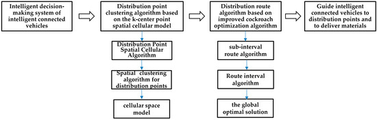
Figure 2.
The constructed intelligent connected vehicle distribution route model.
(1) The introduction section analyzes the research background, the current status, and the existing problems of intelligent connected vehicle material distribution routes. It also analyzes the representative studies conducted by relevant scholars, then proposes our modeling idea, and discusses the research’s architecture.
(2) The distribution point clustering algorithm based on the k-center point spatial cellular model is constructed. The clustering algorithm constructs the neighborhood relationship between the distribution centers and distribution points, providing a spatial data basis for constructing distribution route algorithms.
We determine this method for the following reasons:
① The problem of material distribution involves various geographic information factors such as distribution centers, distribution points, urban roads, spatial distances, etc., and is a complex problem under the constraints of the urban geographic space. Therefore, we choose a cellular model suitable for spatial clustering to construct the clustering algorithm. A cellular unit is a grid dynamics model with a discrete time, space, and state. It has the ability to simulate the spatiotemporal evolution process of complex systems. The expansion and evolution characteristics of cellular units are suitable for constructing a relationship model for dots with spatial attributes. The constructed model involves spatial attributes and spatial relationships, thus, traditional clustering algorithms cannot be used to construct the attributed intimacy relationship. Thus, a cellular clustering method that can establish spatial intimacy is needed.
② Constructing a cellular space with k number of central points conforms to the reality in which the distribution centers in the city serve as the starting points for material reserves and distributions. Clustering algorithms can be used to determine the spatial relationship between distribution centers and distribution points within a neighborhood, providing the precondition for determining and matching an optimal distribution center.
(3) A distribution route algorithm based on the improved cockroach optimization algorithm is constructed, which includes two parts: the station sub-interval route algorithm based on the cockroach optimization algorithm and the distribution route algorithm based on the cockroach optimization algorithm. The route-searching algorithm is used to output the distribution route for each distribution center, in order to determine the optimal distribution center. The process of constructing the route optimization algorithm fully integrates the feature of symmetry in the distribution route problem. We determine this method for the following reasons:
① After determining the spatial clustering relationship between the distribution center and the distribution points, it is necessary to find out the optimal distribution center for the target distribution points, and the selection of the optimal distribution center must be based on the optimal distribution route cost. Therefore, we construct an improved cockroach optimization algorithm to search for the global optimal route within the distribution sub-intervals and the distribution interval, using the distribution center with the optimal route cost as the solution.
② The cockroach optimization algorithm is a high-performance bionic algorithm with a simple modeling process, strong global optimization ability, fast computational speed, and proper algorithm parameters, making it particularly suitable for route-searching problems with cross loops. Compared to other bionic algorithms, the advantage of the cockroach optimization algorithm lies in:
(I) The cockroach optimization algorithm uses a 2-opt mode to obtain step size when generating new individuals. Each time a 2-opt operation is performed, a new cockroach individual is generated. Our designed improved cockroach optimization algorithm has an innovative definition, which defines a cockroach individual as a sub-interval path or a distribution route, while the two points participating in the 2-opt operation are defined by road nodes or distribution points. Therefore, different pathways allow for crossing or “back and forth” states. In real-world logistics distribution problems, vehicles may encounter situations such as transportation route intersections, round-trip routes, and overlapping routes. Compared with other bionic algorithms, the cockroach optimization algorithm is more suitable for this mode.
(II) The cockroach optimization algorithm is suitable for small-scale dataset operations, with a fast computation speed and low time complexity. We make improvements to the traditional cockroach optimization algorithm. First, the 2-opt method is used to continuously generate new cockroach individuals. Second, the individual cost comparison method is used to output the current optimal individual. Third, all cockroaches continue to search for more optimal individuals and they complete the substitution when they crawl towards the optimal individuals. The above three processes are all linear processes with fast convergence speeds. In addition, we perform dimensionality reduction in the search for distribution routes, then the algorithm is divided into two levels: sub-interval searching and distribution interval searching. First, we search for the optimal cockroach individual in the sub-interval to obtain the optimal path in each sub-interval. Then, we search for the optimal cockroach individual in the distribution interval to ultimately obtain the optimal distribution route. In this aspect, it can be seen that the constructed improved cockroach optimization algorithm, through dimensionality reduction and linear processing, does not have internal loop iteration and can effectively reduce the complexity of the computation time. Other bionic algorithms typically require multiple iterations and have high time complexity.
(III) Other heuristic searching algorithms that can be used for route optimization include the fruit fly optimization algorithm, the particle swarm optimization algorithm, the ant colony optimization algorithm, the simulated annealing algorithm, etc. Each heuristic searching algorithm has its own characteristics. From the perspective of algorithm basic principles, the principles of other heuristic searching algorithms are more complex than that of the cockroach optimization algorithm, and they do not have the 2-opt step replacement searching mode for individuals that the cockroach optimization algorithm has. Compared to the cockroach optimization algorithm, the other heuristic searching algorithms are not that suitable for the material distribution route in the scenario proposed by our research work.
(4) Case experiments are designed to verify the algorithm for constructing intelligent connected vehicle material distribution routes. Experimental results show that our proposed algorithm can output routes with the lowest transportation costs, and compared to the commonly used electronic maps and optimization algorithms for distribution route planning, our proposed route algorithm has more advantages than the control group, resulting in lower route costs.
1.4. The Superiority and Contribution of the Proposed Work
1.4.1. The Superiority of the Proposed Work
Compared to the existing methods, our proposed material distribution route algorithm has advantages in its strategy and modeling process, which are mainly reflected in the following aspects.
(1) Multiple distribution centers distributed in cities all have the function of reserving and distributing materials. Under the same functional conditions, selecting the distribution center with the best spatial neighborhood relationship with the distribution points can obtain the optimal matched distribution center and effectively control transportation costs. At present, most of the existing studies on material distribution routes do not consider the precondition of matching distribution centers, and do not search for the optimal distribution route from the perspective of urban geospatial conditions and distribution point neighborhood relationships. The method we have constructed has advantages in this issue, in which we use the clustering algorithm to determine the spatial relationship between distribution centers and distribution points, and use the optimization algorithm to determine the matched optimal distribution center. It can obtain the optimal distribution center and distribution route in the entire urban geographic space.
(2) In real-world logistics businesses, commercial electronic maps are usually used for navigation and route planning. Commercial electronic maps have drawbacks in planning distribution routes, as they are usually based on convenient driving and ferrying. The planned routes connect the city’s primary roads and major road nodes, which might overlook accessible secondary roads and nodes. Therefore, the distribution routes obtained by commercial map planning may not be the global optimal solution. Our proposed method can effectively solve this problem by dividing the distribution route into multiple sub-intervals and constructing a global optimal algorithm within each sub-interval. The subinterval contains all roads and nodes, and the searched route is the global optimal route.
(3) The method we constructed is an improvement on the cockroach optimization algorithm. Compared to other bionic searching algorithms, the cockroach optimization algorithm is more suitable for route searches which randomly select nodes or have intersecting paths. In the basic principle of the cockroach optimization algorithm, the defined step size algorithm when cockroaches crawl towards the optimal individual is a typical 2-opt pattern, which randomly exchanges two nodes in the modeling space and generates a new cockroach individual through the 2-opt step, corresponding to a new feasible path or route. By searching for all the feasible cockroach individuals within the modeling area, the global optimal solution is ultimately obtained.
(4) In addition to bionic searching algorithms, representative route-searching algorithms include the Dijkstra and A* algorithms. These two algorithms are also commonly used as map-searching algorithms for commercial applications, but they have certain drawbacks. Dijkstra is a local, greedy searching algorithm that only considers the current optimal point and ignores the global optimal solution. Therefore, it might not be able to find the global optimal solution and has a high time complexity. The A* algorithm is a heuristic searching algorithm that integrates an evaluation function. When there are too many nodes, the searching process is very cumbersome, with high time complexity. Moreover, when the evaluation function is inaccurate or improper, it might not find the optimal solution. In contrast, the method we constructed can search for the global optimal solution with low time complexity.
(5) In actual logistics business, large-scale logistics distribution problems are often involved. For example, when a large number of distribution points encounter an emergency situation, or when there is a centralized shortage of materials, or when all distribution points in the city need materials, it is necessary to mobilize all distribution centers in the city for material distribution. At present, the existing research methods lack optimization-matching methods for distribution centers, making it difficult to match the optimal distribution center for different distribution points during large-scale logistics distribution, and to quickly search for the optimal distribution route from different distribution centers. The method we have constructed can effectively solve this problem by using a clustering algorithm to obtain neighborhood relationships between distribution points and distribution centers. By quickly searching for routes to match the optimal distribution center for the distribution points, it can obtain a centralized large-scale distribution with multiple distribution centers and optimal routes, and it can achieve the material distribution for multiple distribution points in the shortest time and at the lowest cost.
(6) Compared to other methods which only consider one-way vehicle travel forming a one-way route, our constructed algorithm fully integrates the feature of symmetry in distribution routes, and vehicles generate the same route cost for on and off trips within sub-intervals and distribution intervals.
1.4.2. The Contribution of the Proposed Work
The main contributions of our proposed method are as follows.
(1) We develop an innovative research method and application system that deeply integrates a logistics system with vehicle networking technology, which enhances the intelligence level of logistics distribution systems. We develop a new clustering algorithm, a distribution center-matching algorithm, and a distribution route-searching algorithm, all of which are innovative algorithms in logistics distribution. They provide new methods for academic research in the field of logistics, as well as an executable modeling process reference for the development of new logistics and distribution systems.
(2) Establishing distribution point clusters based on the spatial cellular unit can effectively build the spatial neighborhood relationship between distribution centers and distribution points, and control transportation costs. By searching for the shortest distribution route for each distribution center and combining this with spatial cellular clustering results, we construct a distribution center algorithm that can determine the optimal distribution center for distribution points and provide a new method for logistics distribution.
(3) The constructed improved cockroach optimization algorithm is an innovative method built by combining geospatial constraints, practical logistics, and distribution problems. We divide the distribution route into multiple sub-intervals, and use the sub-interval micro-geospatial environment as the modeling condition to construct a global optimal route algorithm within the sub-interval. Then, we use the distribution interval composed of distribution points as the geospatial environment to construct the global optimal route. This mode is more accurate than commercial map-searching algorithms and can obtain the global optimal route. Meanwhile, compared to the traditional route-searching algorithms of Dijkstra and A*, it has lower time complexity.
2. The Distribution Point Clustering Algorithm Based on the k-Center Spatial Cellular Model
The goal of constructing an intelligent connected vehicle material distribution route algorithm is to optimize the sub-interval route between stations, ultimately making the overall distribution route optimal, minimizing energy consumption and saving on operating costs. Therefore, the precondition for establishing an optimal distribution route algorithm is to construct a spatial relationship model between the distribution centers and the distribution points, so as to optimize the spatial positions of the distribution points and the distribution centers on the route. In this section, we construct a distribution point clustering algorithm based on the k-center spatial cellular model, it introduces the spatial cellular model and the spatial accessibility model, and we perform neighborhood distribution center clustering on the distribution points in the city [25,26,27,28].
2.1. Distribution Point Cellular Space Model Based on the Neighborhood Topology Algorithm
The precondition for the spatial clustering of the distribution points is to construct a cellular space based on the geospatial constraints, in order to establish the micro-spatial relationship between the distribution points and the neighboring road nodes. The cellular unit composed of the distribution points and the neighboring road nodes has a road adjacency relationship, that is, the cellular unit generated by road nodes is connected to the neighboring cellular unit through a common side road. The cellular space is formed by the topology of all the distribution points in the urban space. The cellular space is a geospatial structure model for constructing the spatial clustering algorithm for distribution points.
Definition 1.
The distribution point spatial cellular unit is and the cellular unit control point is . The distribution points in the urban geographic space have spatial attributes such as longitude and latitude, spatial distance, and an adjacency relationship. The closed convex polygonal space formed by the distribution point and the nearest road nodes in the neighboring micro-space is defined as the distribution point spatial cellular unit , in which the distribution point is the core of the unit. All neighboring nodes that make up a cellular unit are defined as the cellular unit control point , in which represents the unit number and represents the No. control point of the unit. According to the definition, the cellular unit and its control point satisfy the following conditions:
(1) The number m of the control points meets , ;
(2) The distribution point does not intersect with any edge ;
(3) There is only one distribution point core within the cellular unit;
(4) The distribution point sends a ray in any outward direction, and the number of intersection points formed by ray and the cellular unit boundary must be an odd number;
(5) The area of the cellular unit region composed of control points is the minimum value .
Any spatial cellular units that satisfy and meet the following conditions:
(1) The cellular unit number meets ;
(2) Cellular regions and meet ;
(3) Any edge of a cellular unit and the other edge of a cellular unit satisfy , if they are not in an adjacency relationship.
Definition 2.
The cellular unit searching azimuth is and the azimuth increasing arc is . Starting from the due north direction of the distribution point , rotate the searching radius clockwise at a uniform angular velocity around the cellular unit. Stop the search when the nearest road node is found. If it is determined that the road node is a cellular unit control point , record the angle between the searching radius and the due-north direction. This angle is defined as the cellular unit searching azimuth , and the uniform angular velocity is defined as the azimuth increasing arc .
Definition 3.
The distribution point cellular space is . The number of distribution points in the urban geographic space are used to generate an number of cellular units with the dispersed relationship or the shared edge , and the cellular units without shared edges are expanded and formed, which generate the adjacency relationship of all the cellular units. Ultimately, the entire urban geographic space is transformed into the cellular space from the number of cellular units that include all distribution points , main roads, and cellular unit control points . According to the definition, the cellular space satisfies the following conditions:
(1) Any cellular unit must be adjacent to another unit or , ;
(2) Any cellular unit control point must belong to at least two cell edges simultaneously;
(3) In space , there are number of cellular units containing distribution points and number of empty cellular units ;
(4) There is no discrete cellular unit .
According to the relevant definitions of the cellular space, we construct a distribution point cellular space model based on the neighborhood topology algorithm (Algorithm 1). The control parameters of the model are determined as follows:
- There are an number of distribution points , consisting of distribution points in the urban domain and located at the cellular center.
- There are a number of control road nodes , which is determined by searching for road nodes around the distribution point, and they are the basic control points that make up the cellular unit.
- The azimuth increasing arc is a fixed angular velocity specified for searching control points.
- The cellular topological edge is a line segment that connects control points in a clockwise motion. It is the finite boundary that constitutes the cellular topology.
The algorithm process is as follows, and Figure 3 shows the modeling process:
| Algorithm 1: The distribution point cellular space model based on the neighborhood topology algorithm |
| Step 1: Identify an number of distribution points and a number of control road nodes in the urban geographic space. The distribution point has the geospatial coordinates and . Road nodes have the coordinates and . |
| Step 2: Select distribution point . Randomly and uniformly select a number of the road nodes within buffer zone , construct a two-dimensional coordinate system with distribution point as the origin, and encode all nodes of the node set in the order of values from small to large while encoding values from large to small. The encoding steps are as follows: |
| (1) Construct a node matrix with the row rank satisfying and the column rank satisfying ; |
| (2) The encoding of the node is , in which represents the row number and represents the column number. Take the node with the largest value and the lowest value, it is encoded as and stored in the matrix element ; Set the counter for row and column as , , with an initial value of . |
| (3) Keep , searching for the second node in the direction of the increasing values, denoted as , and count . Continue to search for the maximum value and determine: |
| ① If , the storage and encoding for the first row of the matrix are completed; jump to Step (4); |
| ② If , the first row of the matrix is stored. For the remaining number of nodes, jump to the execution in condition ③ of Step (4). |
| (4) Note , keep , . Take the node with the smallest value in the row, encode it as , and store it in the matrix element . Search for the second node in the direction of increasing values, denoted as , and count . Continue to search for the maximum value and determine: |
| ① If , the storage and encoding for the second row of the matrix are completed; jump to Step (5); |
| ② If , the second row of the matrix is stored. For the remaining number of nodes, jump to the execution in condition ③ of Step (5). |
| ③ If there are remaining nodes in the row , store the remaining number of nodes to the second row; |
| (5) Note , store the remaining rows in the same way. Take the node with the smallest value in the row, encode it as , and store it in the matrix element . Search for the second node in the direction of increasing value, denoted as , count . Continue to search for the maximum value and determine: |
| ① If , the storage and encoding for No. row of the matrix are completed, continue searching and storing the next row; |
| ② If , the storage for the No. row of the matrix is completed, for the remaining number of nodes, jump to the next row for storage; |
| ③ If there are remaining nodes in the row , store the remaining number of nodes to the No. row. |
| Step 3: Set the encoding matrix as an Open list and construct a Closed list to store the set of cellular unit control points for . Build the distribution point cellular unit . |
| (1) Set the initial scanning line in the positive direction (due north) of the axis based on the origin of the coordinate system , and search for the control point in a clockwise direction along the arc with an increasing azimuth angle , as shown in Figure 4a. |
| (2) Search for the node closest to the axis; according to the definition, it is determined that could be a feasible control point, denoted as , and the current searching azimuth is denoted as . Delete from the Open list and store it in the Closed list, as shown in Figure 4b. |
| (3) The scanning line continues to search in a clockwise direction with an increasing arc . Find , , and , and make a judgment based on: |
| ① The scanning line finds the point , at which point , , and form a closed convex polygon. Temporarily store , and the area is recorded as ; |
| ② The scanning line finds the point , at which point , , , and form a closed convex polygon. Compare and get , delete , and temporarily store ; |
| ③ The scanning line finds the point , at which point , , , and form a closed convex polygon. Compare and get , delete , and temporarily store . Till now, the current area is the smallest, thus, is a feasible control point, denoted as , and the searching azimuth is denoted as . Delete from the Open list and store it in the Closed list, as shown in Figure 4c; |
| (4) The scanning line continues to search in a clockwise direction with an increasing arc , and finds . The area is judged to be a concave polygon but does not meet the conditions for the cellular unit. Exclude , as shown in Figure 4d; |
| (5) The scanning line continues to search in a clockwise direction with an increasing arc , and finds . Judge that conforms to the conditions and is a feasible control point, denoted as . The searching azimuth is denoted as . Delete from the Open list and store it in the Closed list, as shown in Figure 4e; |
| (6) In line with Steps (1) through (5), determine whether the area of the closed polygon is the minimum value, and whether the polygon is convex. Finally, the nodes , , and meet the requirements of the cellular unit. Delete them from the Open list and store them in the Closed list to form the cellular unit. A shown as Figure 4f, the algorithm ends. |
| Step 4: Use the same algorithm process as that in Step 2 and Step 3 to form an number of distribution point cellular units and determine the current status of each unit. Suppose that the geospatial coverage area of a given city domain is , then judge: |
| (1) If , the generated number of cellular units after the topology completely cover the geographical space of the city domain, forming the cellular space, and the algorithm ends; |
| (2) If , the generated number of cellular units after the topology cannot completely cover the geographical space of the city domain. Then, a spatial cellular topology is applied to the non-topological area to generate a number of adjacent empty cellular units , so that the urban domain and the cellular units satisfy Formula (1), forming the cellular space . The algorithm ends. |
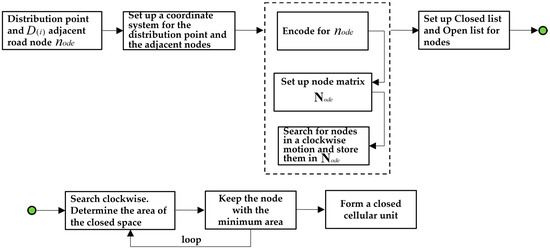
Figure 3.
The constructing process of the distribution point cellular space model based on the neighborhood topology algorithm. The green color circle is used to connect the two steps “Set up Closed list and Open list for nodes” and “Search clockwise. Determine the area of the closed space”.

Figure 4.
The constructed model to form a spatial cellular unit. (a) represents the original status of the searching. (b) represents the searching for the node 3. (c) represents the searching for the node 4, 6 or 7, and decide the proper node. (d) represents the searching for the proper one in node 7, 10 or 11. (e) represents the proper node 7 and 10 are selected. (f) represents the final formed cellular unit. The red circle represents the origin of the coordinate system.
Figure 5 shows the formation process of the cellular space . Figure 5a shows the distributions of the number of points and the number of road nodes , Figure 5b shows the topological state of each distribution point when forming the cellular space, and Figure 5c is the initial cellular space composed of the number of topological cellular units , represented by the green ranges. Figure 5d shows the formed cellular space with the topological empty cellular units. The grey range represents the empty cellular unit. The range within the red dashed line represents the cellular space.
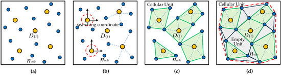
Figure 5.
The formation process of the cellular space. (a) represents the layout of the distribution points and road nodes. (b) represents the forming of the coordinate system and topological state of each distribution point. (c) represents the initial cellular space composed of the topological cellular units. (d) represents the formed cellular space with the topological empty cellular units. The yellow circle represents the distribution point. The blue circle represents the road node. The green space represents the cellular unit with distribution point. The grey space represents the empty cellular unit.
2.2. The k-Center Cellular Clustering Algorithm Based on the Spatial Decision Tree
The distribution centers and distribution points are both the geographical entities distributed in the urban space, with geographical attributes such as spatial coordinates, spatial distance, absolute positioning, and relative positioning. The route through which the distribution vehicles transport materials from the distribution centers to the multiple distribution points is a direct factor in generating transportation costs. Therefore, the constraint for constructing a material distribution route algorithm is to explore the spatial relationship between the distribution centers and the distribution points, visualize and regularize the aggregation relationship between the distribution points and the distribution centers, and prepare the spatial data for constructing a distribution route algorithm with the lowest cost consumption. We introduce the spatial accessibility model and establish a k-center cellular clustering algorithm based on the spatial decision tree [29,30,31,32].
Definition 4.
The absolute coordinates of the target positioning points. The distribution point in the urban geographic space is , and the distribution center is . The distribution center and the distribution point are both defined as the target positioning points, with coordinates denoted as , in which represents the longitude of the target point and represents the latitude of the target point. The coordinates of distribution centers are set as , and the coordinates of distribution points are set as .
Definition 5.
The target point spatial accessibility is . There is an accessibility obstacle caused by the spatial distance between two target points and in the geospatial space, that is, the moving process from the target point to the target point requires paying for the distance cost. Therefore, the distance cost between the target point and the target point is defined as the spatial accessibility cost, and the reciprocal of the spatial accessibility cost is defined as the target point spatial accessibility, denoted as . Formula (2) represents the constructed spatial accessibility model of the target points and , while Formula (3) represents the spatial accessibility model between the distribution center and the distribution point . The parameters in Formulas (2) and (3) are the normalized parameters.
Definition 6.
Distribution point clustering space and distribution point cluster . The total space composed of cellular space , number of distribution centers, and number of control points and connecting roads in the urban geographic space is defined as the distribution point clustering space, denoted as . According to the constructed clustering algorithm, the number of the distribution point cellular units and the empty units in the space are gathered according to a certain rule, so that the cellular units with close spatial attributes are clustered into the same group, while cellular units with distant spatial attributes are discretized into different groups.
Thus, the clustering algorithm is defined to aggregate the cellular units in the urban space, and the group formed by aggregating cellular units with close spatial attributes is defined as a distribution point cluster, denoted as , while specifying the number of clusters generated by the algorithm as . According to the definition, the clusters generated by the algorithm meet the following conditions.
- (1)
- ;
- (2)
- , ;
- (3)
- ;
- (4)
- ;
- (5)
- Adjacent and are connected by at least one shared edge.
Definition 7.
For defining clustering objective function , the criterion for determining whether an object could be included in the cluster of object by the clustering algorithm is whether object has a certain degree of closeness in the feature attributes that meet the constraints. The criterion function for determining this degree of closeness is defined as the clustering objective function, denoted as . When using the spatial attribute closeness as the clustering objective, the function for determining the closeness between object and object is the spatial cost function between the two objects; here, we define it as the target point spatial accessibility . According to the definition, the objective function for constructing the target point cluster is shown in Formula (4), which is transformed to the clustering objective function for the distribution points, as shown in Formula (5), in which the parameters are the normalized parameters.
Definition 8.
For defining the clustering spatial decision tree , when there are multiple cluster objects in the geographic space, the process of determining the inclusion of object to object is the iterative comparison of the clustering objective function. We set up a clustering spatial decision tree to construct an iterative algorithm for incorporating the object into the object . The clustering spatial decision tree meets the following conditions:
(1) The layer where the root node is located is defined as the first layer. When the height of the tree is , the layer where the underlying node is located is the No. layer;
(2) The objective function of any No. layer node is larger than that of the No. layer node, ;
(3) Each node derives, at most, two child nodes, while at least, there could be no child node;
(4) For any No. layer, the objective function of the left node is larger than that of the right node ;
(5) The number of nodes in any No. layer meets .
Definition 9.
Distribution point clustering matrix . We construct the distribution point clustering matrix for the clusters and the intra-cluster distribution points generated in the clustering process. The clustering matrix is used to dynamically store each cluster and its distribution points, and meets the following conditions:
(1) The row rank of the cluster is , the column rank is , in which is the number of clusters, and is the maximum number of distribution points in the cluster;
(2) Any row represents one cluster , and any column represents the No. distribution point;
(3) Any row must have a non-linear correlation with another row , and any column must have a non-linear correlation with another column , ;
(4) The first element of the row where cluster is located stores the growing seed point, while the other elements store the distribution point elements.
According to Definitions 2.1–2.6, we construct a k-center cellular clustering algorithm based on the spatial decision tree (Algorithm 2). The control parameters of the model are determined as follows:
- The spatial accessibility parameter is used to normalize the calculated spatial accessibility, with specific values determined by the calculated spatial accessibility.
- Cluster parameter is determined by the number of distribution centers.
- The decision tree height is determined by the number of distribution centers.
The algorithm process is as follows, and Figure 6 is the algorithm flowchart:
| Algorithm 2: The k-center cellular clustering algorithm based on the spatial decision tree | |
| Input: The number of distribution point cellular units , number of distribution centers , distribution point coordinates , distribution center coordinates . | |
| Output: The number of clusters . | |
| Step 1: Select the number of distribution centers as the growing seed points, establish a dimensional clustering matrix , and store the No. distribution center to the first element of the No. row of . | |
| Step 2: For the number of distribution point cellular units , take and establish the spatial decision tree for the first distribution point . | |
| (1) Take the distribution center corresponding to the No. 1 element in the first row of the matrix and calculate the objective function of and ; | |
| (2) Store in the root node of the decision tree ; | |
| (3) Take the distribution center corresponding to the No. 1 element in the second row of the matrix , calculate the objective function of and , and judge: | |
| ① If , store in the left node of the second layer of the tree; | |
| ② If , store in the left node of the second layer of the tree; | |
| (4) Take the distribution center corresponding to the No. 1 element in the third row of the matrix , calculate the objective function of and , compare, and judge the following: | |
| ① Take and store in the root node of the decision tree; | |
| ② Take and store in the right node in the second layer of the decision tree; | |
| ③ Take the intermediate value and store in the left node of the second layer in the decision tree. | |
| (5) Using the same algorithm as that in Steps (1) through (4), take the distribution center corresponding to the No. 1 element in the No. i row of the matrix , calculate the objective function of and , compare , , …, , determine and store the decision tree through the following steps: | |
| ① Store in the root node of the decision tree; | |
| ② Store in the No. element of the No. layer in the decision tree. The code of meets Formula (6): | |
| (6) | |
| ③ Sort , , …, in descending order, and store them to the decision tree nodes . The storage conditions meet the decision tree rules. | |
| (6) Output a visual decision tree , with the current root node storing the objective function as , corresponding to the distribution center ; | |
| (7) Store in the second element of the related row corresponding to the distribution center in the clustering matrix . | |
| Step 3: For the number of distribution point cellular units , take and establish the spatial decision tree for the second distribution point . The root node of the decision tree stores the objective function , corresponding to the distribution center . Judge the second element of the related row corresponding to the distribution center in the clustering matrix : | |
| (1) If , store in ; | |
| (2) If , store in . | |
| Step 4: Generate a distribution point spatial decision tree by using the same algorithm from Step 2 through Step 3, judge the root node objective function corresponding to the distribution center , store into the No. element of the related row corresponding to the distribution center , and this must meet the following requirements: | |
| (1) If , numerical values can be stored; | |
| (2) If , the No. element must be a non-zero element. | |
| Step 5: Traverse the elements , and store all the distribution points in the corresponding elements of the matrix . For the remaining elements, store a value of 0. The algorithm ends, output the clusters . | |
| Step 6: Connect the edges of the same cluster distribution points in the cellular space , form a boundary connected cluster , and visualize the result. | |

Figure 6.
The constructing process of the k-center cellular clustering algorithm based on the spatial decision tree. The green circle represents the connection of the two steps “Calculate the objective function of distribution points and distribution centers” and “Build decision tree”.
3. Intelligent Connected Vehicle Material Distribution Route Model Based on Improved Cockroach Optimization Algorithm
3.1. Modeling Idea and Relative Definition
In the process of material distribution, the intelligent connected vehicle travels from the distribution center to the number of target distribution points . The process from the first distribution point to the No. distribution point requires passing through several city roads, which will result in route costs and energy consumption. From the perspective of cost saving and an energy consumption reduction, the process of intelligent connected vehicles starting from a distribution center , transporting materials to a number of distribution points , and finally returning to the distribution center , requires minimizing route costs. Based on the geographical constraints, the starting point of the intelligent connected vehicle distribution route is , the middle points are the number of distribution points , and the terminal point is , which forms a complete closed interval [33,34]. Based on the principle of distribution route modeling and the characteristics of the distribution route, it can be concluded that vehicles depart from the distribution center, pass through several target distribution points, and finally return to the distribution center. The whole process forms a complete route with the feature of symmetry, that is, the generated route costs of the on and off trips are identical. According to basic modeling conditions, the material distribution route we construct needs to meet the following conditions:
(1) The starting point and the number of distribution points are discrete points in space, with no concatenation in their respective cellular units ;
(2) The number of distribution points could be the cellular units within the different clusters , and the starting point must belong to, and only belongs to, a unique cluster ;
(3) Any two points, such as and or and , are directly or indirectly connected by urban roads;
(4) Intelligent connected vehicles do not turn back when moving between any two points, such as and or and ;
(5) The sub-interval routes generated by the movement of intelligent connected vehicles between any two points such as and or and can have intersections or partial overlaps;
(6) The closed route consists of the starting points , distribution points , and road nodes .
Based on the construction conditions of the distribution routes combined with the urban geospatial constraints, we set up an intelligent connected vehicle material distribution route algorithm based on the improved cockroach optimization algorithm. For the number of distribution points , we select the distribution center with the best spatial distribution and the function to optimize the distribution route. It enables intelligent connected vehicles to make decisions on the optimal material distribution route, minimizing route costs and energy consumption.
Definition 10.
For distribution route sub-interval and distribution route interval , the process of intelligent connected vehicles starting from the initial point , passing through a number of distribution points , and finally returning to the destination constitutes a complete interval. The initial point and distribution points are defined as the control points . If any point and are randomly selected from the number of control points , , the micro-space structure composed of and is defined as the distribution route sub-interval, denoted as , in which and are, respectively, and , represents the sub-interval code. The complete route formed by connecting a number of adjacent sub-intervals in a micro-spatial structure is defined as the distribution route interval, denoted as , and represents the route code. In the geospatial environment, a sub-interval of a route is composed of several roads and road nodes . According to the definition, we obtain the relationship between the sub-interval and the route interval:
(1) contains a number of control points ;
(2) contains a number of sub-intervals , there are ;
(3) When there is a random change in the position of control point in , will immediately change and can generate type of routes, .
Definition 11.
Sub-interval cockroach individual and interval cockroach individual . For any , the intelligent connected vehicle moves from the starting control point to in a sub-interval , and this process randomly passes through number of road nodes , then one feasible path in the sub-interval composed of number of road nodes , as well as the control points to , is defined as a cockroach individual in the sub-interval , denoted as . For any , the intelligent connected vehicle starts from the initial point within the interval , passing through number of distribution points to complete the material distribution and returning to the initial point , the whole process forms a complete path, and this path is defined as an individual cockroach in the interval , denoted as . According to this definition, the sub-interval cockroach individual and the interval cockroach individual meet the following relationship conditions:
(1) The quantity of in the sub-interval is determined by the number of road nodes in the sub-interval;
(2) The quantity of is determined by the number of distribution points , according to the corresponding relationship of , and there is ;
(3) The optimal route for an intelligent connected vehicle within the sub-interval is formed by , and the optimal route within the interval is formed by ;
(4) The geographical constraints for constructing and are the road distance and the cellular unit clusters in the cellular space .
Definition 12.
The cockroach crawling step . According to the foraging characteristics of the cockroach swarm, the process of the cockroach swarm’s crawl towards food (the optimal solution) exhibits the group randomness feature. Within the sub-interval , the crawling step of a cockroach is defined as one replacement operation of road nodes within the sub-interval (a 2-opt operation). Every time the road nodes change, the cockroach moves one step towards the food direction. Within the interval , the crawling step of cockroach is defined as one replacement operation of distribution points within the interval. Each time the distribution points change, the cockroach moves one step towards the food direction. According to the definition, the process of a cockroach crawling towards food is a process of number of replacements on the control points. The step of each replacement is denoted as , and represent the control points. The crawling path of the cockroach meets Formula (7).
Definition 13.
The cockroach initial solution is , the cockroach current solution is , and the cockroach optimal solution is . The initial state of the cockroach or is composed of the control points at the certain time . According to the problem objective, an intelligent connected vehicle will generate the movement distance cost after passing through all the control points in the sub-interval or interval . The movement distance cost generated by the control points at is defined as the cockroach initial solution, denoted as . When the cockroach crawls to the food object by step with the time interval of , the movement cost of the intelligent connected vehicle at time is defined as the cockroach current solution, denoted as . The crawling path of the cockroach from time to time is denoted as . When the cockroach swarm crawl to the food object, after multiple iterations, the finally output cockroach with the smallest distance cost is set as the optimal cockroach, and its corresponding distance is the optimal solution, denoted as . According to the definitions of the sub-interval and the route interval , the optimal solution of the route interval cockroach is the iterative value of the optimal solution of the sub-interval cockroaches. The route interval cockroach model is shown in Formula (8).
Definition 14.
Step disturbance factor . During an iteration process from to , the cockroach swarm crawl from the initial state to the current state . If all the cockroaches have the same current solution, namely , the iteration enters a dormant state. At this moment, a step disturbance factor is introduced to interfere with the state of the cockroaches, causing them to generate a new state and continue crawling to search for the global optimal solution. According to the definition, the step of a cockroach after introducing a step disturbance factor is shown in Formula (9), and the current solution of a new cockroach generated by the step disturbance factor is shown in Formula (10).
Definition 15.
To define the distribution route cost decision tree , build a complete binary tree to store the distribution route cost generated by the cockroaches during their crawling process, and use the complete binary tree to search for the distribution route with the lowest cost. The distribution route cost decision tree meets the following conditions:
(1) The layer where the root node is located is defined as the first layer. When the height of the tree is , the layer where the underlying node is located is the No. layer;
(2) The route cost of any No. layer node is smaller than the route cost of the No. layer node, ;
(3) Each node could derive, at most, two child nodes, and at least, there is no child node;
(4) For any No. layer, the route cost of the left node is smaller than that of the right node ;
(5) The number of nodes in any No. layer meets .
3.2. Modeling Process
According to the modeling idea and objective, we construct an intelligent connected vehicle material distribution route model based on the improved cockroach optimization algorithm, which includes two algorithm modules. The goal of Module 1 is to search for the cockroaches with the optimal solution in each sub-interval of the distribution route, while the goal of Module 2 is to search for the cockroach with the optimal solution in the distribution route interval . Based on the algorithm analysis, we construct algorithms for the two modules, and the Module 1 algorithm is the precondition for the Module 2 algorithm.
The control parameters of the model are determined as follows:
- (1)
- The distribution sub-interval parameters:
- For number of road nodes , collect all accessible nodes within the sub-interval.
- For the node ferrying distance , the ferrying distances between adjacent nodes within the sub-interval are collected.
- For the 2-opt step size, perform one sequential replacement or connection replacement on adjacent road nodes.
- (2)
- The distribution interval parameters:
- A number of control points are composed by the distribution center and distribution points, and both the distribution center and distribution points within the distribution route are the control points.
- The ferrying distance between control points is determined by the optimal cockroach individual output in the sub-interval.
- For the 2-opt step size, perform one sequential replacement or connection replacement of adjacent control points .
The following is the algorithm process for Module 1 and Module 2. Figure 7 shows the algorithm flow of Module 1. Figure 8 shows the process of randomly generating one cockroach within a sub-interval .

Figure 7.
The constructing process of the sub-interval distribution route model based on the improved cockroach optimization algorithm. The green circle represents the connection of the two steps “Form a cockroach individual” and “Form k number of cockroach individuals”. The yellow circle represents the connection of the two steps “The iteration process” and “If all solutions are equal, execute food distribution”.

Figure 8.
The process of randomly generating one cockroach within a sub-interval. (a) represents the initial status of the searching process. (b) represents the searching for the node 1. (c) represents the searching for the node 4. (d) represents the searching for the node 3. (e) represents the searching for the node 6. (f) represents the searching for the node 7. (g) represents the searching for the node 9. (h) represents the searching for the node 11. (i) represents the final route is formed.
The Module 1 Algorithm: a sub-interval distribution route model based on the improved cockroach optimization algorithm (Algorithm 3).
| Algorithm 3: The sub-interval distribution route model based on the improved cockroach optimization algorithm |
| Input: Sub-interval , , the number of road nodes in the sub-interval, the distance between adjacent nodes , the distribution center , and distribution points as control points . |
| Output: The optimal cockroach , the global optimal solution . |
| Step 1: Set the control point as the starting point and the control point as the ending point to construct the first sub-interval and generate the first feasible cockroach . |
| (1) Construct the spatial layout of the control points , , and road nodes , as shown in Figure 8a; |
| (2) Randomly select the neighboring point of , form a path, and store , as shown in Figure 8b; |
| (3) Continue searching in the direction of , randomly select the neighboring point of , form a path, and store , as shown in Figure 8c. Judge point , Path (4,2) forms a turnaround path, discard ; |
| (4) Continue searching in the direction of , randomly select the neighboring point of , form a path, and store , as shown in Figure 8d. Judge point , Path (1,4,3,1) forms a closed path, discard ; |
| (5) Continue searching in the direction of , randomly select the neighboring point of , form a path, and store , as shown in Figure 8e. Judge point , Path (6,5) forms a turnaround path, discard ; |
| (6) Continue searching in the direction of , randomly select the neighboring point of , form a path, and store , as shown in Figure 8f. |
| (7) Judge the points , , and , and whether they form a closed or turnaround path with , discard it; randomly select the neighboring point of , form a path, and store , as shown in Figure 8g; |
| (8) Continue searching in the direction of , randomly select the neighboring point of , form a path, and store , as shown in Figure 8h; |
| (9) Judge point , Path (11,8) forms a turnaround path, discard ; search for , form a path, Path (i, 1,4,3,6,7,9,11, j), and the search processing ends, as shown in Figure 8i. Output the No. 1 cockroach . |
| Step 2: Set the control point as the starting point and the control point as the ending point, and generate the second feasible cockroach in the first sub-interval . |
| (1) Take the first cockroach and select any node ; |
| (2) Search for the nearest neighboring point of that can form a path, and is not the next node of in ; |
| (3) Search for the that is connected to in , as it can form path, store the , and form ; if searching for the point that is connected to out of , a path can also be formed. Turn to Step 1 and search for the subsequent path after the until is reached, the searching ends, form ; |
| (4) Record that the cockroaches complete one instance of crawling . |
| Step 3: Follow the above steps, set the control point as the starting point and the control point as the ending point, and generate the No. feasible cockroach in the first sub-interval . |
| Step 4: Calculate the initial solutions of the number of cockroaches and get the corresponding movement distances along the path . Take the corresponding individual of as the current optimal solution . |
| Step 5: The number of cockroaches crawl towards the current optimal cockroach with the step . Make a judgment based on the following: |
| (1) Crawl for the No. 1 step , calculate the current solutions for the number of cockroaches, and take the corresponding cockroach of as the current optimal solution : |
| ① If , keep as the optimal solution; |
| ② If , replaces , and the current optimal solution is . |
| (2) Crawl for the No. 2 step , calculate the current solutions for the number of cockroaches, and take the corresponding cockroach of as the current optimal solution . Determine the current optimal solution by using the same method as that in Step (1). |
| (3) Crawl for the No. 3 step, No. 4 step, …, No. N step, and judge: |
| ① If at a certain time there are number of cockroaches whose current solutions satisfy , then a step disturbance factor is introduced to randomly allocate a step to the current solutions to generate the new cockroaches and the new current solution . Return to Step (1), the k number of cockroaches continue to crawl and search for the global optimal solution . |
| ② After N iterations, if the output of the iteration result is always a certain cockroach , it is the global optimal solution. The searching ends. |
| Step 6: Output the global optimal solution and the corresponding cockroach . |
| Step 7: Output the optimal cockroaches and global optimal solutions for the remaining number of sub-intervals via the same methods from Step 1 through Step 6. |
The Module 1 algorithm generates the lowest cost for each sub-interval within the intelligent connected vehicle distribution route. Based on the sub-interval cost , we set up the Module 2 algorithm: the distribution route model based on the improved cockroach optimization algorithm (Algorithm 4). Figure 9 shows the algorithm flow of Module 2.
| Algorithm 4: The distribution route model based on the improved cockroach optimization algorithm |
| Input: Sub-interval , , sub-interval route , sub-interval optimal cost , starting point distribution center , and number of distribution points . |
| Output: The optimal cockroach , the global optimal solution . |
| Step 1: The distribution center and the number of distribution points form a number of control points , which can form types of distribution route intervals . |
| Step 2: When generating cockroach , keep the order of in the route unchanged, and step acts on . The step in the whole route interval is one occurrence of the 2-opt operation; |
| Step 3: Randomly arrange number of distribution points to generate the first distribution route interval , corresponding to the cockroach in the first route interval: |
| (1) Confirm the number of sub-intervals for ; |
| (2) Confirm the optimal cost for the number of sub-intervals; |
| (3) Calculate the optimal cost of the cockroach in the interval, corresponding to the cost of the route interval , denoted as ; |
| (4) Store to the root node of the decision tree . |
| Step 4: Randomly arrange a number of distribution points to generate the second distribution route interval , corresponding to the cockroach in the second interval: |
| (1) Confirm a number of sub-intervals for ; |
| (2) Confirm the optimal cost for a number of sub-intervals; |
| (3) Calculate the optimal cost of the cockroach in the interval, corresponding to the cost of the route interval , denoted as ; |
| (4) Compare and , take the and store it in the root node of decision tree ; take the and store it in the child node of the second layer of the decision tree . |
| Step 5: In line with Step 3 through Step 4, generate the cockroach for the No. route interval, calculate the route cost of , and compare , , …, . Store using the storage rule of the complete binary tree, , . |
| Step 6: Take the current cockroach at the root node of the decision tree as the current optimal cockroach, corresponding to the cost . The number of child node cockroaches crawl to the current optimal cockroach by step . Make a judgment based on the following: |
| (1) Crawl for the No. 1 step , calculate the current solutions for the number of cockroaches, and take the corresponding cockroach of as the current optimal solution : |
| ① If , keep as the optimal solution; |
| ② If , replaces , and the current optimal solution is . |
| (2) Crawl for the No. 2 step , calculate the current solutions for the number of cockroaches, and take the corresponding cockroach of as the current optimal solution . Use the same method as that of Step (1) to determine the current optimal solution and replace the decision tree. |
| (3) Crawl for the No. 3 step, No. 4 step, …, No. N step, and judge: |
| ① If at a certain time there are number of cockroaches whose current solutions satisfy , then a step disturbance factor is introduced to randomly allocate a step to the current solutions to generate new cockroaches and the new current solution . Return to Step (1), a number of cockroaches continue to crawl and search for the global optimal solution . Replace the decision tree. |
| ② After N iterations, if the output of the iteration result is always a certain cockroach , it is the global optimal solution. Replace the decision tree. The searching ends. |
| Step 6: Output the global optimal solution and the corresponding cockroach , while also outputting the final decision tree. |

Figure 9.
The constructing process of the distribution route model based on the improved cockroach optimization algorithm. The green circle represents the connection of the two steps “Form k number of cockroach individuals” and “The iteration process”. The yellow circle represents the connection of the two steps “The iteration process” and “If all solutions are equal, execute food distribution”.
4. Experiment and Result Analysis
4.1. Data Collection and Experiment Process
4.1.1. Data Collection
To verify the feasibility and advantages of the proposed method, we design and implement a scenario experiment, and choose Zhengzhou City in Henan Province as the experimental area.
(1) Data Group 1: Based on the geospatial layout characteristics of Zhengzhou city, we confirm the intelligent connected vehicle material distribution centers as and determine the geospatial coordinate set to be . The experimental conditions for the distribution centers are that ① the quantity is , which meets the clustering modeling conditions of cellular space, with , ; ② the whole spatial distribution has the feature of randomness; that ③ they are uniformly distributed within the urban area of Zhengzhou City; and that ④ any two distribution centers are directly or indirectly connected by roads and have the feature of accessibility.
(2) Data Group 2: set the distribution of goods and materials as the experimental scenario, set the large supermarkets in Zhengzhou city that need to receive materials as the distribution points , and determine their coordinate set to be . The experimental conditions for the distribution points are that the ① quantity is , which meets the clustering modeling conditions of the cellular space, with , ; ② they are uniformly distributed within the urban area of Zhengzhou City; ③ any two distribution points are directly or indirectly connected by roads, and they have the feature of accessibility; and that ④ any distribution center is directly or indirectly connected to any distribution point by roads, and they have the feature of accessibility.
(3) Data group 3: there are a number of distribution centers and an number of distribution points with a total number of spatial points . Based on the geographical distribution of the number of spatial points , take any two points and as the sub-interval control points, , . Collect the road nodes between and in the map of Zhengzhou City, and collect the movement distance between any two nodes .
Table 2 shows the four distribution centers and their coordinates set for the experiment; thus, , . Table 3 shows the 10 large supermarkets in Zhengzhou city and their coordinates set for the experiment, denoted as the distribution points ; thus, , . Figure 10a shows the layout of the distribution centers , Figure 10b shows the layout of the distribution points , Figure 10c shows the layout of some major road nodes , and Figure 10d shows the overlay of the distribution centers, distribution points, and major road nodes. Based on the modeling conditions and the experimental requirements, the experimental distribution points we have confirmed are : Zhong Yuan Wanda; : Er Qi Wanda; : Jinyi Cheng; : Xi Yuan Mall; : Renmin Road Dennis; : Er Qi MixC City; : Guomao 360; : Zhengzhou YinxiangHui; : Dennis Outlets; and : Hanhai Beijin.
Table 2.
The distribution centers and coordinates of the experiment.
Table 3.
The distribution points (supermarkets) and coordinates in Zhengzhou city.

Figure 10.
The layout of distribution centers, distribution points, road nodes, and the overlay diagram. (a) represents the layout of the distribution centers. (b) represents the layout of the distribution points. (c) represents the layout of some major road nodes. (d) represents the overlay of the distribution centers, distribution points, and major road nodes.
4.1.2. Experiment Process
Based on the experimental objectives, we design the following experimental process:
(1) Based on the number of distribution points , use the constructed distribution point cellular space model to output the Zhengzhou city cellular space.
(2) Based on the number of distribution centers , the number of distribution points , and the road nodes , the k-center cellular clustering algorithm based on the spatial decision tree is used to calculate the clustering spatial decision tree for each distribution point . The objective functions and the distribution point clustering matrix of each distribution point relative to the distribution center are output, and the spatial clusters of the distribution centers are finally output to determine the distribution points with the highest spatial closeness to each distribution center. Based on the clustering results, output the clustering space .
(3) Based on the clustering results, randomly select the distribution points for the materials to be transported. Weigh the spatial relationship between the point of each cluster and the distribution points , and use the constructed intelligent connected vehicle material distribution route model to search for the optimal route. Starting from the distribution center of each cluster , we search for the shortest route, respectively, and select the distribution center with the lowest route cost as the starting point for distribution.
(4) Design the comparative experiment to verify the advantages of the proposed algorithm. Intelligent connected vehicles usually use electronic maps for route planning. We choose the commonly used Baidu Map (Version: 16.3.0) and 360 Map (Version: 3.7.0.1004) as the control group, and our proposed algorithm is the experimental group, with the selected point as the common starting point. The control group and the experimental group, respectively, output the optimal route, and compare the results of the distance cost and time cost. At the same time, we also set the commonly used route optimization algorithms of Dijkstra and A* as the control group, and the proposed algorithm as the experimental group, to compare the costs generated by the algorithms for the same distribution route. Compare the time complexity of the proposed algorithm, the Dijkstra algorithm, and the A* algorithm.
4.2. Experiment Result Analysis
4.2.1. Result and Analysis on the Distribution Point Cellular Space
Generate a cellular space containing 10 distribution points and certain road nodes within the Zhengzhou city by using the constructed topology algorithm, as shown in Figure 11. Figure 11a shows the extracted of 10 discrete distribution points and all road nodes ; Figure 11b shows the generated cellular space, in which each closed and independent unit consisting of three or more road nodes is a spatial cellular unit. The green cellular unit represents the one in which the distribution point is located, and the white cellular unit represents the empty cellular unit .

Figure 11.
The basic element of the cellular space and the generated cellular space. (a) shows the extracted of 10 discrete distribution points and all road nodes. (b) shows the generated cellular space. in which each closed and independent unit consisting of three or more road nodes is a spatial cellular unit. The green cellular unit represents the one in which the distribution point is located, and the white cellular unit represents the empty cellular unit .
By analyzing the visualization results of the cellular space in Figure 11, the following conclusions can be drawn:
(1) Perform an overlay analysis on the distribution maps of the distribution points and the road nodes. The distribution points and the road nodes show a non-overlapping spatial relationship, which meets the conditions for constructing the cellular space algorithm. For the distribution pattern of point set and , it can be seen that one distribution point can form multiple cellular structures.
(2) Constrained by the geographical space and the road distribution conditions of Zhengzhou city, the constructed cellular space algorithm only generates one optimal cellular distribution structure, and the position, structure, area, and the included points of each distribution point cellular unit and empty cellular unit are controlled and fixed by the algorithm and the geographical constraints.
(3) The cellular space visualizes the relative positions, adjacency relationships and clustering relationships between the distribution point cellular units and the empty cellular units in the spatial coordinate system, forming the necessary condition for distribution point cellular clustering. From the analysis of the adjacency relationship of each cellular unit, it can be concluded that the adjacent cellular units with shared edges are superior to the remote ones in forming a gathered cluster in the aspect of the geographical conditions.
4.2.2. The Results and Analysis of the Distribution Point Cellular Space Clustering
Firstly, the distribution center set is loaded into the distribution point set and the road point set through the overlay operation. The spatial accessibility between each distribution point and the distribution center is calculated based on the spatial coordinates of the point set collected in Table 2 and Table 3, and the clustering objective function is constructed. Output the clustering spatial decision tree of each distribution point using the clustering algorithm, and output the clustering matrix . Based on the matrix , output the clusters with the distribution centers as the k-center points. Figure 12 shows the clustering spatial decision tree of each distribution point. The tree nodes store the objective functions between the distribution point and the distribution center , representing the spatial accessibility between points. The distribution center of the root node is the cluster in which the distribution points are located. Table 4 shows the generated distribution point clustering matrix . According to the decision tree of each distribution point visualized in Figure 12 and the clustering matrix of distribution points in Table 4, the clusters generated by each distribution center are obtained. The results of each cluster are as follows:
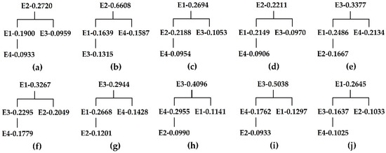
Figure 12.
The clustering spatial decision tree of each distribution point . (a–j) represent the trees of distribution points to .
Table 4.
The generated distribution point clustering matrix .
- (1)
- Cluster : ;
- (2)
- Cluster : ;
- (3)
- Cluster : ;
- (4)
- Cluster : .
Based on the constraints of the clustering algorithm on the control points and the boundary conditions of each cluster in the cellular space, as well as the generated cellular space structure and the clustering results, the cluster shape is generated in the cellular space, which includes cluster centers , cluster cellular units , and road nodes , as shown in Figure 13. Figure 13a is a structural diagram containing the distribution centers and the relationship between each cellular unit and the center . Figure 13b is a structural diagram of each cluster, and the cluster covered by the dark yellow boundaries and the blue area is the cluster where distribution center is located; the cluster covered by the red boundaries and the purple area is the cluster where distribution center is located; the cluster covered by the dark grey boundaries and the gray area is the cluster where distribution center is located. In each cluster, the cluster contains three cellular units, , , and , marked in pink; cluster contains three cellular units, , , and , marked in green; cluster contains four cellular units, , , , and , marked in brown; and cluster contains empty cellular units.

Figure 13.
The generated cluster shape in the cellular space, including the cluster centers , cluster cellular units , and road nodes . (a) is a structural diagram containing the distribution centers and the relationship between each cellular unit and the center. (b) is a structural diagram of each cluster, and the cluster covered by the dark yellow boundaries and the blue area is the cluster where distribution center is located; the cluster covered by the red boundaries and the purple area is the cluster where distribution center is located; the cluster covered by the dark grey boundaries and the gray area is the cluster where distribution center is located.
Based on the analysis of Figure 12 and Figure 13 and Table 4, the following conclusions can be drawn:
(1) The constructed clustering algorithm is effective in aggregating distribution points with spatial attributes, and can achieve clusters based on the spatial accessibility of distribution points. Therefore, the constructed clustering algorithm is feasible for achieving spatial clustering.
(2) Figure 12a–j represent the clustering spatial decision trees of distribution points ~. The clustering spatial decision tree generated for each distribution point corresponds to the spatial accessibility between the distribution point and each distribution center, and there are significant differences in spatial accessibility between the points. Taking Figure 12a as an example, the spatial accessibility between distribution point and distribution centers ~ are visualized in the structural tree-. The spatial accessibility between and that is stored in the root node is 0.2720; the spatial accessibility between and that is stored in the left child node of the second layer is 0.1900; the spatial accessibility between and that is stored in the right child node of the second layer is 0.0959; the spatial accessibility between and that is stored in the child node of the third layer is 0.0933. According to the structural tree-, the algorithm stores in a descending order for spatial accessibility, and the cluster corresponding to the distribution center of the root node is the cluster to which the distribution point belongs. The storage principle of other decision trees ~ is identical.
The quantitative results of the decision tree prove that the constructed clustering algorithm can obtain the spatial relationship between the distribution points and the distribution centers through data-mining methods, and visualizes this spatial relationship through a tree structure. The decision system of intelligent connected vehicles can search for the distribution center with the highest spatial closeness to the current distribution point by using the tree structure, providing a quantitative basis for determining the distribution center with the lowest transportation cost.
(3) In the distribution point clustering matrix , the clusters and both contain three distribution points, while cluster contains four distribution points. This result proves that the clustering algorithm has the feature of fairness and uniformity in constructing the spatial relationship between the distribution points and the distribution centers, and can effectively and fairly cluster each distribution point. The algorithm has strong features of robustness.
(4) In the distribution point clustering matrix , the cellular units contained in cluster are all the empty cellular units. This proves that the constructed clustering algorithm can quickly and accurately search for the noise points with the lowest spatial closeness, and can eliminate the noise points, providing the optimal spatial conditions for intelligent connected vehicles to search for distribution routes.
(5) Analyze the generated shape and layout of the clusters in Figure 13. Figure 13a shows the layout structure of the distribution centers and distribution points in the cellular space. The green area represents the cellular units where the distribution points are located, and the solid yellow circles represent the distribution centers. From the distribution map, it can be seen that there is a relatively discrete spatial relationship between the cellular units of the distribution centers and the distribution points, and there are spatial accessibility barriers between the distribution centers and the distribution points. Therefore, constructing clusters with the distribution centers as coordinate origins is a precondition for obtaining the optimal spatial clustering of distribution points and for searching for the optimal distribution route. Figure 13b shows the visualization results of the clusters output by the algorithm. The blue area represents distribution center cluster , the purple area represents distribution center cluster , and the green area represents distribution center cluster . Distribution center does not constitute a cluster. The spatial accessibility from distribution point contained in its cluster to the distribution center within this cluster is greater than that of the distribution centers within other clusters, indicating that the distribution points of one cluster are closest to the distribution center within this cluster, and the cost of transporting materials from the distribution center within the cluster to the distribution points of the cluster is the lowest. When the distribution points that require materials involve multiple clusters, the closer the cluster is, and the more distribution points belong to it, the higher the probability that its distribution center is output by the algorithm as the starting point of the distribution route. Among the three clusters containing distribution points, and have four shared edges, and have four shared edges, while and do not have shared edges. This proves that the constructed clustering algorithm is constrained by the geographical space and the road traffic conditions, and the clusters are strictly composed of positioning points and road boundaries. The visualization results of the clusters provide decision support for intelligent connected vehicles in searching for routes.
4.2.3. The Results and Analysis of the Intelligent Connected Vehicle Distribution Route
Experiment Condition
Based on the constraints of the operating speed and the material distribution time of intelligent connected vehicles in cities, the following scenarios are set in the experiment, and experimental data is collected based on these preconditions. The experiment outputs intelligent connected vehicle distribution routes.
(1) Constrained by urban transportation and the geospatial conditions, the comprehensive average speed for an intelligent connected vehicle is set to 20 km/h;
(2) When an intelligent connected vehicle arrives at the distribution point at a certain time , it immediately carries out material uploading. When material uploading is completed, it leaves at a certain time to move on to the next point . The experimental sets that, from the time of arrival in to the time of departure in , the intermediate time (in hours) is used for material unloading, and the unloading time met is . For the ease of calculation, we set uniformly. Set the loading time of the intelligent connected vehicle at the distribution center as 8:00–10:00 a.m., and the departure time as 10:00 a.m.
(3) The working time in the whole process of intelligent connected vehicles is jointly determined by the travel time and the uploading time. The experiment sets a maximum of four distribution points for intelligent connected vehicles to deliver materials within a working day of 8 h. Therefore, the number of control points that the distribution route meets is . According to the conditions, the randomly selected distribution points for the experiment are {: Zhong Yuan Wanda; : Jinyi Cheng; : Dennis Outlets; and : Hanhai Beijin}.
(4) Based on the number of the distribution points , and on the route sub-intervals involved in the experiment, the maximum number of the sub-intervals meets .
Experiment Results and Analysis
According to the experimental conditions, we collect the movement distance between all the road nodes and the adjacent nodes in Zhengzhou City. We randomly select the distribution points with a total quantity from each cluster and set them as the control points for the material distribution routes. An intelligent connected vehicle starts from the distribution center , distributes materials to the distribution points along the algorithm constrained route, and finally returns to . Using the constructed improved cockroach optimization algorithm, we firstly output the global optimal cockroaches between the control points containing and by using the Module 1 algorithm, and then determine the optimal solutions of the sub-intervals , which are the shortest road travel distances in the sub-intervals. Secondly, using the Module 2 algorithm, we search the route intervals composed of and to obtain the global optimal cockroach , and determine the optimal solution of the interval , which is the shortest moving distance of the distribution route.
According to the experimental conditions and process, we output the cockroach , the sub-interval cost , and cockroach cost corresponding to the optimal distribution route starting from ~ (also ending at ~), as shown in Table 5. Based on the results in Table 5, we visually output the trend charts of the sub-interval costs and the interval cost corresponding to the optimal cockroach cost in the sub-interval and the optimal cockroach cost in the route interval, as Figure 14 shows. Figure 14a–d represents the optimal distribution routes from the distribution centers ~ as the starting (and ending) points, with the blue curve representing optimal route 1 and the red curve representing optimal route 2.
Table 5.
The cockroach , sub-interval cost , and cockroach cost corresponding to the optimal distribution route starting from ~ (also ending at ~).

Figure 14.
The trend charts of the sub-interval costs and the interval cost corresponding to the optimal cockroach cost of the sub-interval and the optimal cockroach cost of the route interval. (a–d) represent the charts for Starting (Ending) point ~.
Based on the results in Table 5 and Figure 14, it can be seen that by selecting the distribution points in each cluster, among all the optimal routes starting from the distribution centers ~ (also endpoints), the two distribution routes starting from the distribution center (also an endpoint) have the lowest cost of 35.1, followed by the two distribution routes starting from the distribution center (also an endpoint) with a cost of 36.1. The costs of distribution routes starting from and (also endpoints) are relatively high, at 41.0 and 41.7, respectively. Therefore, the intelligent connected vehicle system selects distribution center as the starting point for material distribution, and chooses or . Table 6 shows the operation time schedule, the total time consumption, and the total mileage of the intelligent connected vehicle completing material distribution from the starting point (also the endpoint) based on the results output in Table 5, in which represents the departure time and represents the arrival time. The experimental results show that when using the same algorithm with different starting distribution centers, there are significant differences in the costs of the distribution routes. Choosing the distribution center with the lowest route cost as the starting point for distribution can effectively reduce the distribution cost for the intelligent connected vehicles.
Table 6.
The operation time schedule, total time consumption, and total mileage of an intelligent connected vehicle completing material distribution from the starting point (also endpoint). In the table, CP—control point, TS—time schedule, TC—time consumption (unit: h), RM—route mileage (unit: km).
Figure 14 shows that when starting from any distribution center, the cost of the route interval shows a fluctuating trend. When the starting points are identical, the interval costs of the two routes are different, but the final route costs are the same. When using the same distribution center as the starting point, the total costs of the on and off routes are the same, but due to the different costs of each interval, the time schedules for the distribution vehicles to arrive at each distribution point are different. This result can also be obtained from Table 6. It indicates that when delivering materials, the two modes can be selected based on the different time requirements and the urgency of each distribution point: the on and off routes. The relatively urgent distribution points can be arranged for morning distribution, while the relatively less urgent distribution points can be arranged for afternoon distribution. This result also fully demonstrates the feature of symmetry in our proposed algorithm, as the driving costs for vehicles in the on and off trips in the distribution routes are identical.
4.2.4. Comparative Experiment and Analysis
Experiment Condition
To verify the feasibility and advantages of the proposed algorithm, we select commercial electronic maps, which are most frequently used for route planning in logistics distribution, as the control group, including the Baidu Map and the 360 Map. The control experiment conditions are set as follows:
(1) Set the comprehensive average speed for the intelligent connected vehicle to 20 km/h;
(2) Based on the experiment in Section 4.2.3, determine to be the optimal distribution center. Therefore, in the comparative experiments, the routes all start and end at distribution center , with the distribution order set as “-Route 1”, that is, the route is “”;
(3) The loading time for the intelligent connected vehicle at the distribution center is from 8:00 a.m. to 10:00 a.m., and the departure time is 10:00 a.m. The uploading time for each distribution point is ;
(4) Using the same route as the standard, the control group determines the shortest route within each sub-interval of the distribution route by using the Baidu Map and the 360 Map as the searching method, outputs the cost of each sub-interval and the total cost of the route, and based on this, outputs the distribution time schedule for the experimental group and the control group.
(5) The commonly used route-searching algorithms embedded in electronic maps include the Dijkstra optimization algorithm, the A* optimization algorithm, etc. They are classic methods in searching for the shortest route. On the basis of comparing the commonly used map methods for route planning, we use the Dijkstra optimization algorithm and the A* optimization algorithm for the control group to compare with our proposed route algorithm, including the route cost and computational complexity.
Results and Analysis of the Comparison with Commonly Used Map Methods
Based on the comparative experimental conditions and objectives, we output the sub-interval costs and route costs on the same distribution route for the experimental group and the control group, as shown in Table 7. The experimental group is represented as EG, the Baidu Map method for the control group is represented as CG-1, and the 360 Map method for the control group is represented as CG-2. Based on the results in Table 7, we obtain the sub-interval cost and total route cost curves and comparison charts for the experimental group and the control group on the distribution route, as shown in Figure 15. Figure 15a shows the sub-interval cost and total route cost for the experimental group, Figure 15b shows the sub-interval cost and total route cost for the Baidu Map method, Figure 15c shows the sub-interval cost and total route cost for the 360 Map method, and Figure 15d is the comparison bar chart between the results of the experimental group and those of the control group, in which the blue bar represents the experimental group, the yellow bar represents the Baidu Map method, and the green bar represents the 360 Map method. Based on the results of the comparative experiment, the time cost and time schedules for the three methods of distributing materials are output according to the distribution requirements, as shown in Table 8.
Table 7.
The sub-interval costs and the total route costs output by the experimental group and the control group.

Figure 15.
The curve chart and the comparative chart of the generated sub-interval costs and total route costs in the same distribution route for the experimental group and control group. (a) represents the experimental group. (b) represents the control group 1. (c) represents the control group 2. (d) represents the comparison among the experimental group, control group 1 and control group 2.
Table 8.
The time cost and time schedules for the three methods of distributing materials. In the table, CP—control point, TS—time schedule, TC—time consumption (unit: h), RM—route mileage (unit: km).
Analyzing Table 7 and Figure 15, under the conditions of the two sets of route planning methods for the experimental group and the control group, the sub-interval cost and route cost of the three methods show a fluctuating trend, indicating that our proposed algorithm and map methods are constrained by the urban geographic space when planning distribution routes, resulting in different transportation costs in the different sub-intervals. Analyzing the sub-interval costs, our proposed algorithm generates lower distances and time costs in the vast majority of sub-intervals than the routes planned by the control group, and the total costs of the routes are also lower than the routes planned by the control group. Experimental results show that our proposed algorithm has significant advantages in searching for the lowest cost route compared to the commonly used electronic map methods for distribution route logistics planning. The global optimal route obtained from the searching process can generate lower distances and time costs than the electronic maps.
In terms of the total route cost, the proposed algorithm has a distance cost 1.2 km lower than the Baidu Map method and 2.7 km lower than the 360 Map method. In terms of the total time cost, the proposed algorithm has a time cost 0.06 h lower than the Baidu Map method and 0.135 h lower than the 360 Map method. The experimental results demonstrate that our proposed algorithm can search for the global optimal distribution route and minimize the cost of distribution routes. Therefore, as for the operating vehicle in the logistics distribution system, the intelligent connected vehicle is controlled by the backend server decision-making system. The proposed algorithm could serve as an embedded guiding algorithm to lead an intelligent connected vehicle, which can minimize transportation costs. Take a practical application scenario for example: assuming that the fuel or electricity consumption per 1 km of vehicle travel is constant, when multiple distribution vehicles participate in distributing activities for multiple times, if our proposed algorithm saves 1 km of transportation route costs in a single distributing activity compared to conventional map methods, then 1000 occurrences of distributing activities can save 1000 km of transportation route costs. Converting this into fuel or electricity, it can save logistics companies from a huge amount of energy consumption and significant expenses. From the perspective of energy conservation, our proposed algorithm has significant advantages over map-planning methods.
Results and Analysis of the Comparison with Route-Searching Algorithms
The Dijkstra optimization algorithm and the A* optimization algorithm are set as the control group. We output the sub-interval costs and route costs on the same distribution route for the experimental group and control group, as shown in Table 9. The experimental group is represented as EG, the Dijkstra optimization algorithm for the control group is represented as CG-1, and the A* optimization algorithm for the control group is represented as CG-2. Based on the results in Table 9, we obtain the curves of the sub-interval costs and the total route costs, and comparison charts for the experimental group and the control group on their distribution routes, as shown in Figure 16. Figure 16a shows the sub-interval costs and the total route cost of the experimental group, Figure 16b shows the sub-interval costs and the total route cost of the Dijkstra optimization algorithm, Figure 16c shows the sub-interval costs and the total route cost of the A* optimization algorithm, and Figure 16d is the comparison bar chart between the experimental group and the control group, in which the blue bar represents the experimental group, the yellow bar represents the Dijkstra optimization algorithm, and the green bar represents the A* optimization algorithm.
Table 9.
The sub-interval costs and route costs of the distribution route for the experimental group and control group.
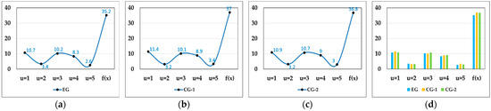
Figure 16.
The curve chart and comparative chart of the generated sub-interval costs and total route costs in the same distribution route for the experimental group and control group. (a) represents the experimental group. (b) represents the control group 1. (c) represents the control group 2. (d) represents the comparison among the experimental group, control group 1 and control group 2.
Based on the proposed algorithm modeling process and principle, we calculate the time complexity of the proposed algorithm, the Dijkstra optimization algorithm, and the A* optimization algorithm, and then obtain the comparison results in Table 10. In terms of time complexity, is the number of road nodes within the sub-interval or the number of control nodes in the distribution route.
Table 10.
The comparison of the time complexity of the proposed algorithm, the Dijkstra optimization algorithm, and the A* optimization algorithm.
Analyze the results of Table 9 and Figure 16. Under the conditions of the two groups of route-planning methods, the sub-interval costs and the route costs of the output routes of the three methods all show a fluctuating trend, indicating that our proposed algorithm and the two route optimization methods are constrained by the urban geographic space when planning distribution routes, resulting in different costs in different sub-intervals. By analyzing the costs of the sub-intervals, it can be seen that our proposed algorithm generates lower costs in the vast majority of sub-intervals than the routes in the control group, and the total cost of the routes is also lower than that of the routes in the control group. The experiment proves that our proposed algorithm has advantages over the two route optimization algorithms in searching for the lowest-cost route, and the global optimal route obtained from the searching process can generate lower costs. Under the example conditions, the distance generated by our proposed algorithm is 1.8 km lower than that of the Dijkstra algorithm, while the total distribution time is 0.09 h lower; the distance generated by our proposed algorithm is 1.6 km lower than that of the A* algorithm, while the total distribution time is 0.08 h lower.
Analyze the reasons for this result. Firstly, Dijkstra is a locally greedy searching algorithm that focuses only on the optimal solution of the current node in each searching step, rather than searching for the route from a global optimal perspective. Especially when the number of nodes in the searching interval is large, Dijkstra’s ability to search for the global optimal solution is not outstanding. A* has strict requirements for the selection of an evaluation function, it is sensitive to the estimated path cost, and may not be able to search for the global optimal solution. In contrast, our proposed algorithm is an improvement on the cockroach optimization algorithm, which is divided into sub-intervals and route intervals. Each level establishes an optimal solution algorithm that traverses all cockroach individuals, ensuring that the global optimal solution can be searched for within both sub-intervals and route intervals. Therefore, its performance is better than that of Dijkstra and A*. From the perspective of time complexity, we have improved the cockroach optimization algorithm by reducing its originally complex dimensionality and changing its multi-loop structure, while calculating the optimal solution separately in sub-intervals and route intervals. It greatly reduces time complexity. Dijkstra is based on local greedy searching and A* is inspired by evaluation function searching. Their algorithm models include two-level loop structures, and the more nodes there are, the higher the time complexity will be. Therefore, the computational efficiency of our proposed algorithm is higher.
4.3. Conclusions on the Problem Solutions
Through these experiments, we have verified the feasibility of the constructed material distribution route algorithm and its advantages compared to other methods. Based on the experimental results, we identify solutions to the problems of material distribution outlined in Section 1.2 and Figure 1 in the introduction, as shown in Figure 17.
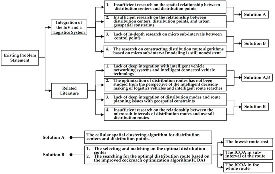
Figure 17.
The solutions to the problems obtained by the algorithm modeling and experimental analysis.
5. Conclusion and Prospect
5.1. Research Conclusions
On the basis of analyzing the problems in the material distribution routes, we propose a research method to integrate the intelligent connected vehicle system with material distribution, and construct an intelligent connected vehicle material distribution route model based on k-center spatial cellular clustering and the improved cockroach optimization algorithm. By establishing a cellular space based on distribution centers, distribution points, and geospatial data, a k-center spatial cellular clustering algorithm is constructed to generate spatial clusters with the distribution centers as the clustering seed points. The neighborhood relationship between the distribution centers and the distribution points is quantified and visualized. Based on the neighborhood relationship, an intelligent connected vehicle material distribution route model based on the improved cockroach optimization algorithm is constructed. The goal is to search for the optimal distribution route starting from each distribution center, compare the costs of the distribution routes from each distribution center using the spatial decision tree, and obtain the optimal distribution center recommendation. To verify the feasibility and advantages of the algorithm, we design case studies and comparative experiments. Experimental results show that our proposed algorithm has a total distance cost that is 1.2 km lower than the distance cost generated by the Baidu Map method and 2.7 km lower than the distance cost generated by the 360 Map method. In terms of the total time cost, it is 0.06 h lower than the time cost generated by the Baidu Map method and 0.135 h lower than the time cost generated by the 360 Map method. Therefore, our proposed algorithm can search for the distribution route with the lowest transportation cost. Compared to the commonly used electronic maps for distribution route-planning, our proposed algorithm can output distribution routes with lower costs than the electronic maps under the same distribution sequence, ultimately reducing the transportation costs for the intelligent connected vehicle material distribution system. Compared with the commonly used Dijkstra algorithm and A* algorithm for route optimization, our proposed algorithm also generates lower costs. Under the example conditions, the distance generated by our proposed algorithm is 1.8 km lower than that of the Dijkstra algorithm, and the total distribution time is 0.09 h less than that of the Dijkstra algorithm. The distance generated by our proposed algorithm is 1.6 km lower than that of the A* algorithm, and the total distribution time is 0.08 h less than that of the A* algorithm.
5.2. The Scope of Its Practical Application
The proposed distribution route algorithm has rigorous logic and executable capability, and has a wide range of applications in the logistics field, mainly including the following aspects.
(1) The clustering model constructed with a distribution center as the core can be applied to the spatial distribution and layout planning of distribution points, serving as the basis for management departments to formulate decision-making plans and related policies.
(2) The distribution center-matching method based on distribution route cost can be applied to site selection of distribution centers, providing a scientific and quantitative basis for management departments, helping them to select the optimal distribution center and quickly make material distribution decisions.
(3) The constructed distribution route algorithm can be used for urban conventional logistics distribution route planning, emergency material distribution route planning, etc., providing a scientific basis for management departments to quickly design transportation routes.
(4) All the constructed algorithms, including the spatial clustering algorithm, the distribution center-matching algorithm, and the distribution route algorithm, are the deep integration of intelligent vehicle networking technology and logistics technology. They can be used as embedded algorithms for developing intelligent systems such as vehicle decision-making systems, navigation systems, management information systems, and material distribution decision-making systems, etc., providing technical support for system research, development, and application.
5.3. Future Work
The material distribution route algorithm is based on fixed distribution centers and distribution points, without considering the urgency of material demand at different distribution points. In future research, the urgency of material requirements at distribution points can be considered as an important factor in the planning of distribution routes. For distribution points that urgently need supplies, they can be arranged to receive morning distribution, while other distribution points can be arranged to receive distributions at a later time period. Integrating urgency to construct a route algorithm can make the intelligent connected vehicle decision-making system more personalized and adaptable to possible emergency situations in material distribution. In addition, the location selection of distribution centers is also an important issue in the field of material distribution research. Based on the spatial modeling method and the route-searching algorithm we have developed, establishing a distribution center location algorithm for the urban geographic space and the optimal distribution scenarios will also be the focus of our subsequent research. Optimizing the layout of distribution centers can further optimize the space for material distribution, thereby improving the efficiency of material distribution and reducing transportation costs.
Author Contributions
Conceptualization, X.Z., J.W. and W.L.; methodology, X.Z., W.L. and J.P.; formal analysis, W.L., J.P., T.Z., F.J. and R.L.; visualization, J.P., T.Z. and R.L.; writing—original draft preparation, X.Z., J.W. and W.L.; writing—review and editing, X.Z., J.W., J.P., T.Z. and F.J.; funding acquisition, J.W. and W.L. All authors have read and agreed to the published version of the manuscript.
Funding
This research was funded by the Research on Army Equipment Damage Prediction Model (No. LJ20212C031089).
Data Availability Statement
Data are contained within the article.
Conflicts of Interest
The authors declare no conflicts of interest.
Abbreviation
| Distribution point spatial cellular unit | |
| Cellular unit control point | |
| Cellular unit searching azimuth | |
| Azimuth increasing arc | |
| Distribution point cellular space | |
| Absolute coordinates of target positioning points | |
| Target point spatial accessibility | |
| Distribution point clustering space | |
| Distribution point cluster | |
| Clustering objective function | |
| (a) | Clustering spatial decision tree |
| Distribution point clustering matrix | |
| Distribution route sub-interval | |
| Distribution route interval | |
| Sub-interval cockroach individual | |
| Interval cockroach individual | |
| Cockroach crawling step | |
| Cockroach initial solution | |
| Cockroach current solution | |
| Cockroach optimal solution | |
| Step disturbance factor | |
| (b) | Distribution route cost decision tree |
References
- Brusselaers, N.; Fredriksson, A.; Gundlegård, D.; Zernis, R. Decision support for improved construction traffic management and planning. Sustain. Cities Soc. 2024, 104, 105305. [Google Scholar] [CrossRef]
- Xie, D.; Qiu, Y.; Huang, J. Multi-objective optimization for green logistics planning and operations management: From economic to environmental perspective. Comput. Ind. Eng. 2024, 189, 109988. [Google Scholar] [CrossRef]
- Tajik, M.; Tosarkani, B.; Makui, M.; Ghousi, R. A novel two-stage dynamic pricing model for logistics planning using an exploration–exploitation framework: A multi-armed bandit problem. Expert Syst. Appl. 2024, 246, 123060. [Google Scholar] [CrossRef]
- Andrés, R.; Jesús, G.; Michelle, R. A spatio-functional logistics profile clustering analysis method for metropolitan areas. Transp. Res. Part E 2023, 179, 103312. [Google Scholar]
- Seiran, H.; Lina, K. A stochastic microscopic based freeway traffic state and spatial-temporal pattern prediction in a connected vehicle environment. J. Intell. Transp. Syst. 2024, 28, 313–339. [Google Scholar]
- Wang, W.; Liu, Y.; Dai, Y.; He, Y. Joint cooperative caching and power control for UAV-assisted internet of vehicles. Sci. Rep. 2024, 14, 9341. [Google Scholar] [CrossRef]
- Danchuk, V.; Comi, A.; Weiß, C.; Svatko, V. The optimization of cargo delivery processes with dynamic route updates in smart logistics. East.-Eur. J. Enterp. Technol. 2023, 2, 64–73. [Google Scholar]
- Da, Z.Y.; Yang, W.J.; Ran, P.P.; Qian, X.G.; Shao, S.; Pan, S.; Shi, B.J.; Li, Y.; He, R.L.; Xiao, Y.H. Design of Logistics Route Planning for Printing Enterprises Based on Baidu Map. In ITM Web of Conferences; EDP Sciences: Les Ulis, France, 2017; Volume 11, p. 10001. [Google Scholar]
- Ma, Z.; Zhang, J.; Wang, H.; Gao, S. Optimization of Sustainable Bi-Objective Cold-Chain Logistics Route Considering Carbon Emissions and Customers’ Immediate Demands in China. Sustainability 2023, 15, 5946. [Google Scholar] [CrossRef]
- Ni, C.; Dohn, K. Research on Optimization of Agricultural Products Cold Chain Logistics Distribution System Based on Low Carbon Perspective. Int. J. Inf. Syst. Supply Chain Manag. 2024, 17, 1–14. [Google Scholar] [CrossRef]
- Chen, L.; Shen, Z. Logistics Path Decision Optimization Method of Fresh Product Export Cold Chain Considering Transportation Risk. Comput. Intell. Neurosci. 2022, 2022, 8924938. [Google Scholar] [CrossRef]
- Chen, J.; Liao, W.; Yu, C. Route optimization for cold chain logistics of front warehouses based on traffic congestion and carbon emission. Comput. Ind. Eng. 2021, 161, 107663. [Google Scholar] [CrossRef]
- Xu, W.; Rong, M. Research on Optimization of Expressway Logistics Path Based on the Advantages of Multimodal Transport in the Environment of Internet of Things. Wirel. Pers. Commun. 2021, 126, 1981–1997. [Google Scholar] [CrossRef]
- Dang, F.L.; Wu, C.X.; Wu, Y.; Li, R.; Zhang, S.; Jiaying, H.; Liu, Z.G. Cost-based multi-parameter logistics routing path optimization algorithm. Math. Biosci. Eng. 2019, 16, 6975–6989. [Google Scholar] [CrossRef] [PubMed]
- Zhu, C.; Zhang, Z.; Wang, Q. Path Choice of Emergency Logistics Based on Cumulative Prospect Theory. J. Adv. Transp. 2019, 2019, 8512423. [Google Scholar] [CrossRef]
- Nie, W.; Chu, L.; Xiang, N.; Liu, Y. Research on distribution mode of urban rail logistics and optimization of node location. Chin. J. Undergr. Space Eng. 2023, 19, 17–25. [Google Scholar]
- Wang, S.; Zhu, X.; Shang, P.; Lin, X.; Yang, L.; Tavasszy, L. Two-echelon multi-commodity multimodal vehicle routing problem considering user heterogeneity in city logistics. Expert Syst. Appl. 2024, 252, 124141. [Google Scholar] [CrossRef]
- Reusken, M.; Laporte, G.; Rohmer, S.; Cruijssen, F. Vehicle routing with stochastic demand, service and waiting times—The case of food bank collection problems. Eur. J. Oper. Res. 2024, 317, 111–127. [Google Scholar] [CrossRef]
- Zhao, S.; Li, P.; Li, Q. The Vehicle Routing Problem Considering Customers’ Multiple Preferences in Last-Mile Delivery. Teh. Vjesn. 2024, 31, 734–743. [Google Scholar]
- Polimeni, A.; Vitetta, A. Network design and vehicle routing problems in road transport systems: Integrating models and algorithms. Transp. Eng. 2024, 16, 100247. [Google Scholar] [CrossRef]
- Kumar, N.; Sood, S.; Saini, M. Internet of Vehicles (IoV) Based Framework for electricity Demand Forecasting in V2G. Energy 2024, 297, 131199. [Google Scholar] [CrossRef]
- Zhu, S.; Tian, X.; Chen, H.; Zhu, H.; Qiao, R. Edge collaborative caching solution based on improved NSGA II algorithm in Internet of Vehicle. Comput. Netw. 2024, 244, 110307. [Google Scholar] [CrossRef]
- Shu, Y.; Zhu, F.; Zhang, Z.; Zhang, M.; Yang, J.; Wang, Y.; Wang, J. Graph embedded low-light image enhancement transformer based on federated learning for Internet of Vehicle under tunnel environment. Comput. Intell. 2024, 40, e12648. [Google Scholar] [CrossRef]
- Hai, T.; Aksoy, M.; Iwendi, C.; Ibeke, E.; Mohan, S. CIA Security for Internet of Vehicles and Blockchain-AI Integration. J. Grid Comput. 2024, 22, 43. [Google Scholar] [CrossRef]
- Sany, L.; Lucas, S. Nearly tight bounds on the price of explainability for the k-center and the maximum-spacing clustering problems. Theor. Comput. Sci. 2023, 949, 113744. [Google Scholar]
- Shang, Q.; Yu, Y.; Xie, T. A Hybrid Method for Traffic State Classification Using K-Medoids Clustering and Self-Tuning Spectral Clustering. Sustainability 2022, 14, 11068. [Google Scholar] [CrossRef]
- Pouya, B.; Mehdi, F.; Kate, S.; Vladimir, E. A transformation technique for the clustered generalized traveling salesman problem with applications to logistics. Eur. J. Oper. Res. 2020, 285, 444–457. [Google Scholar]
- Heredia, C.; Moreno, S.; Yushimito, W. ODMeans: An R package for global and local cluster detection for Origin–Destination GPS data. SoftwareX 2024, 26, 101732. [Google Scholar] [CrossRef]
- Plante, J.; Radatz, M. On the Capability of Classification Trees and Random Forests to Estimate Probabilities. J. Stat. Theory Pract. 2024, 18, 25. [Google Scholar] [CrossRef]
- Wu, J.; Li, C. Illustrating the nonlinear effects of urban form factors on transportation carbon emissions based on gradient boosting decision trees. Sci. Total Environ. 2024, 929, 172547. [Google Scholar] [CrossRef]
- Cassiano, B.; Tobias, S.; Annegret, H. Spatial constraints in cellular automata-based urban growth models: A systematic comparison of classifiers and input urban maps. Comput. Environ. Urban Syst. 2024, 110, 102118. [Google Scholar]
- Zeng, H.; Wang, H.; Zhang, B. An urban cellular automata model based on a spatiotemporal non-stationary neighborhood. Int. J. Geogr. Inf. Sci. 2024, 38, 902–930. [Google Scholar] [CrossRef]
- Pustiulha, S.; Samchuk, V.; Holovachuk, I.; Prydiuk, V.; Klak, Y. Methodology for Selecting Optimal Routes for the Transportation of Dangerous Goods in Conditions of Risk Uncertainty. Transp. Telecommun. J. 2024, 25, 150–160. [Google Scholar] [CrossRef]
- Aronshtam, L.; Sand, B.; Shrot, T.; Cohen, R.; Levin, C.; Daltrophe, H. Optimal Route Crowd-Shipping System for Sustainable Rapid Delivery: Algorithm, Simulation, and Feasibility Evaluation. Future Transp. 2023, 4, 1–14. [Google Scholar] [CrossRef]
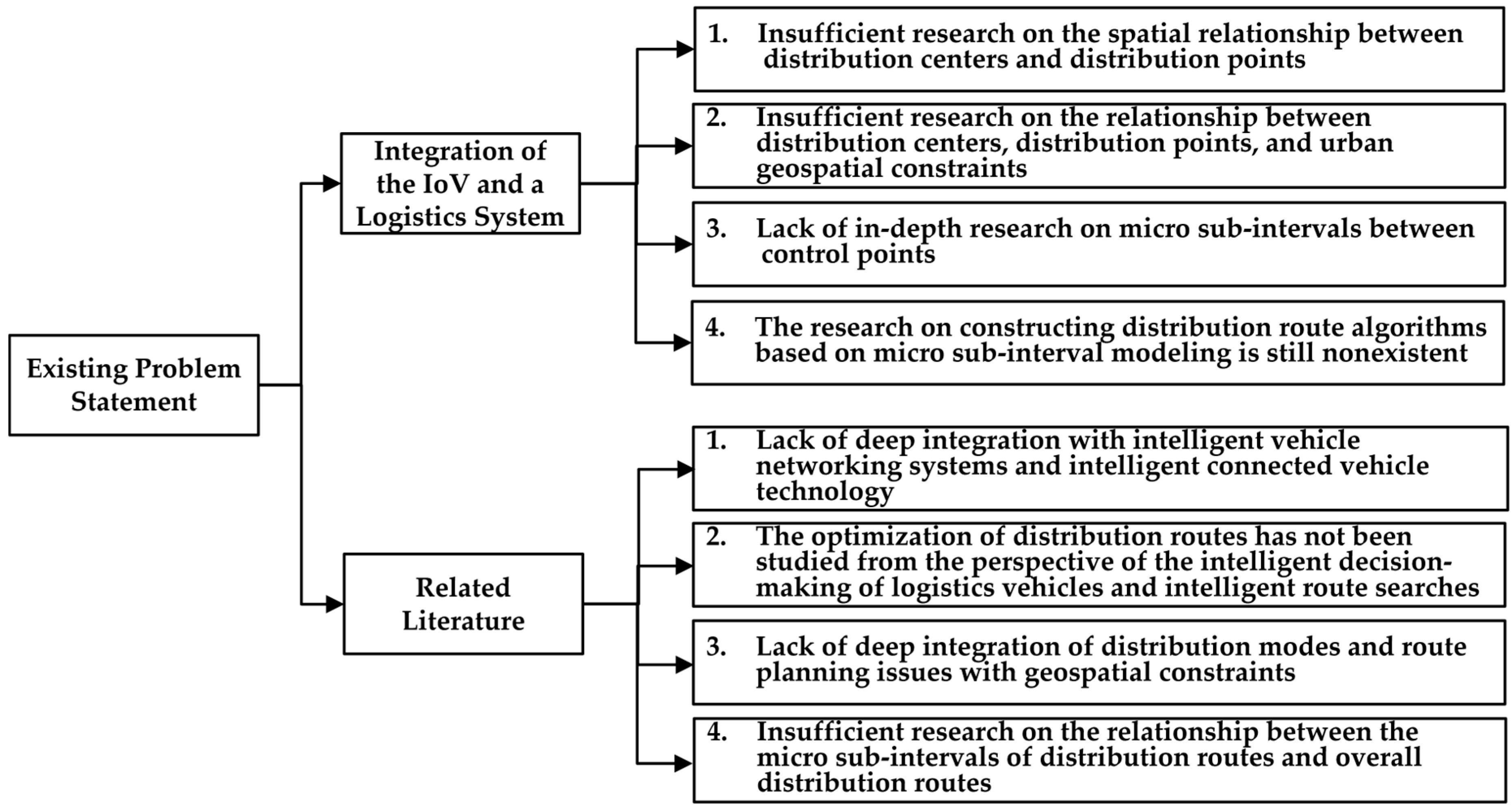
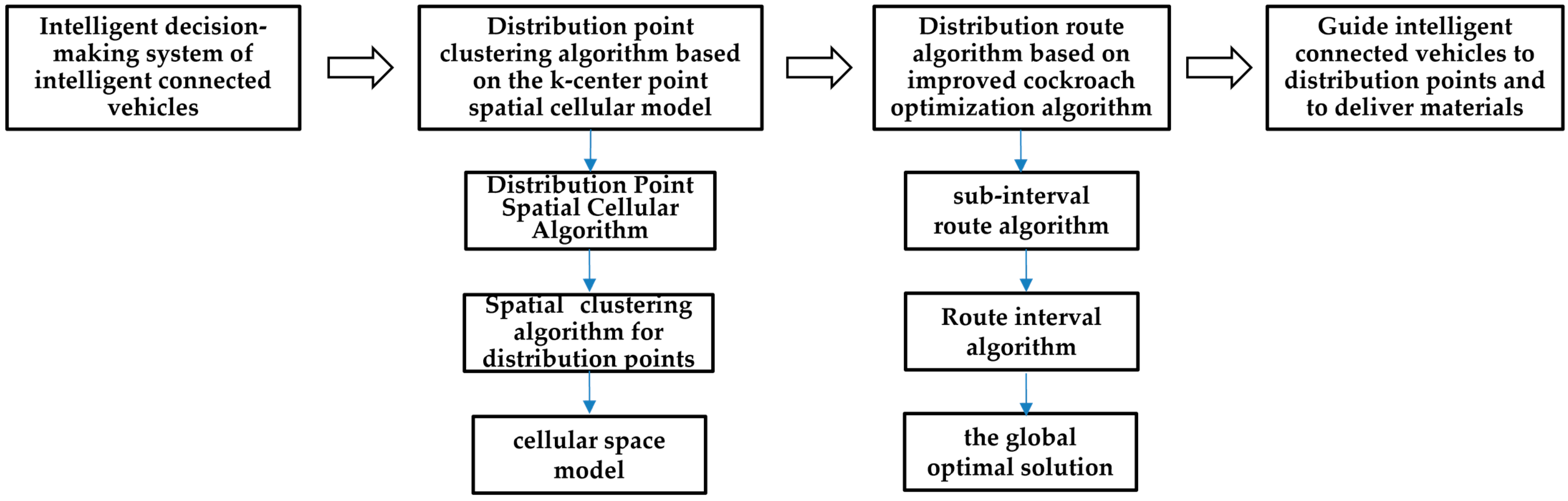

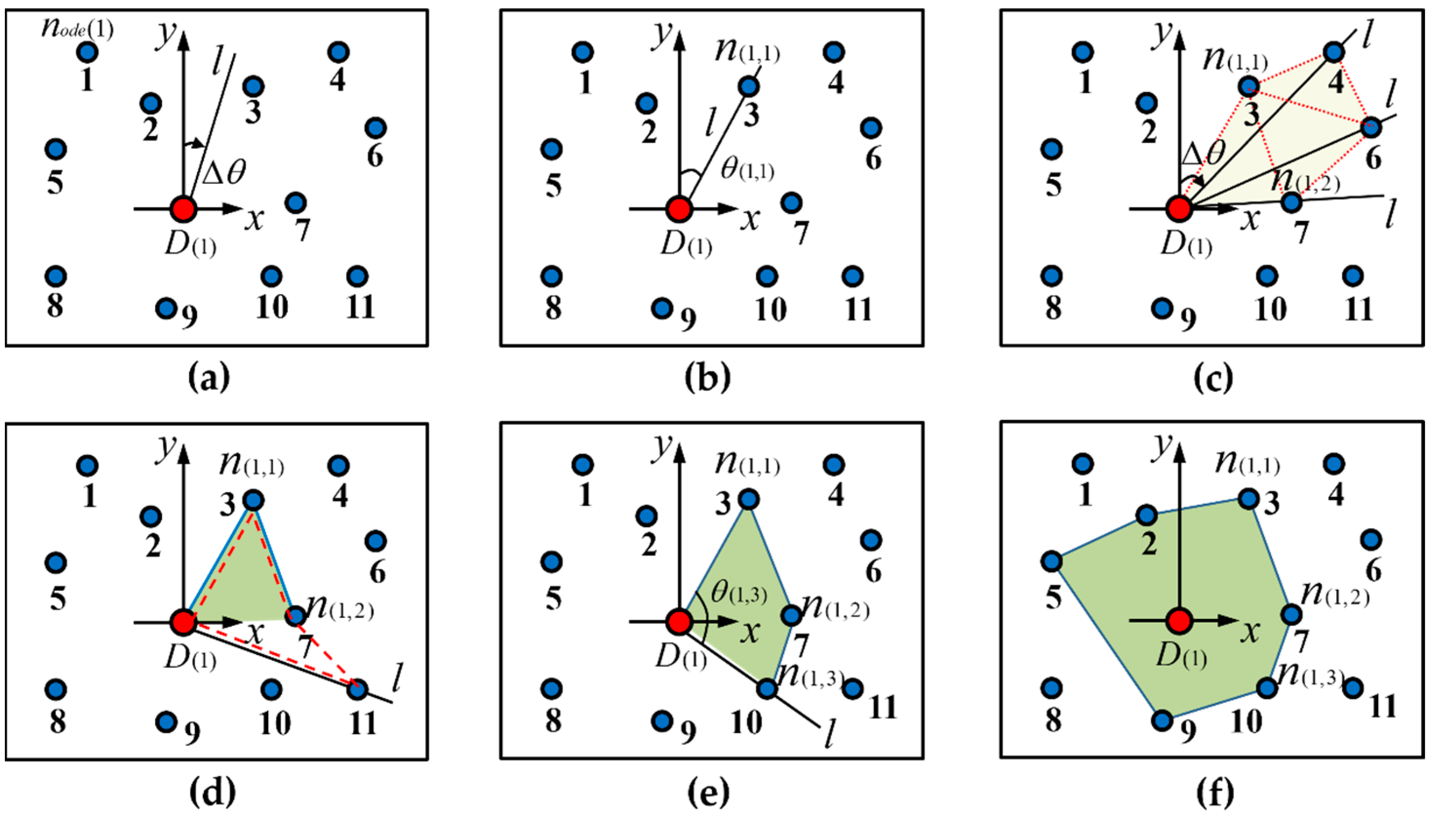
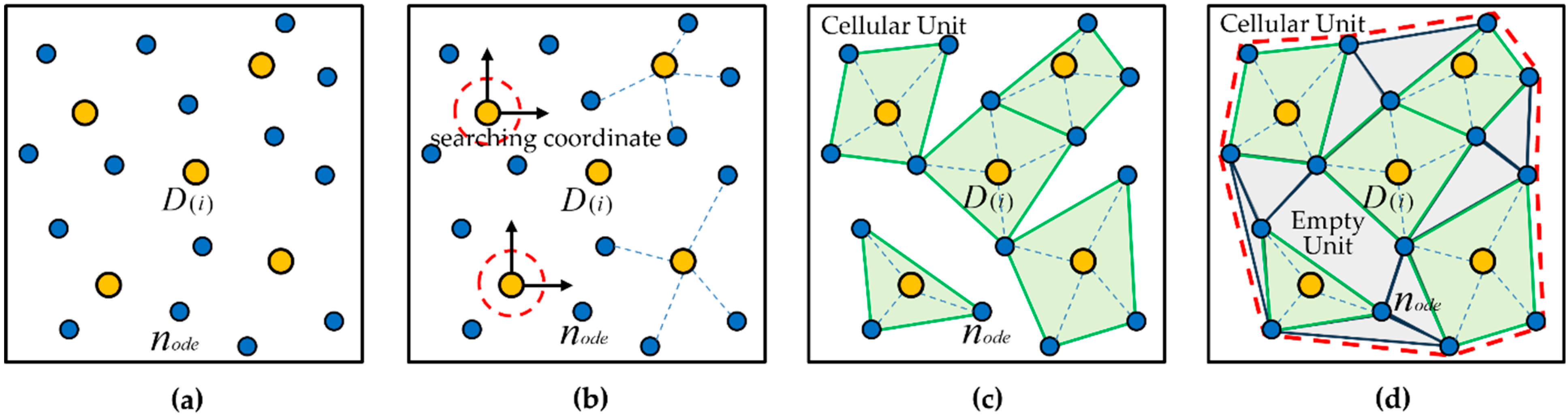
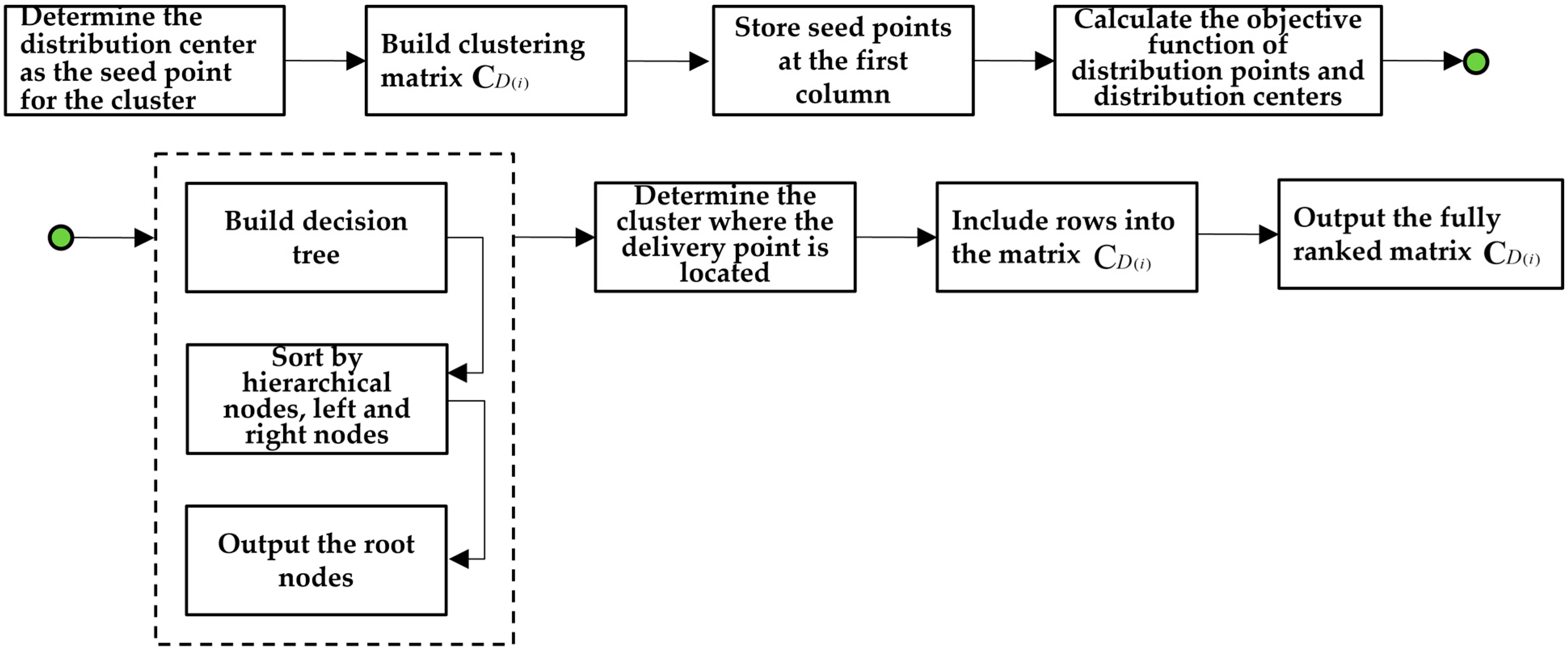
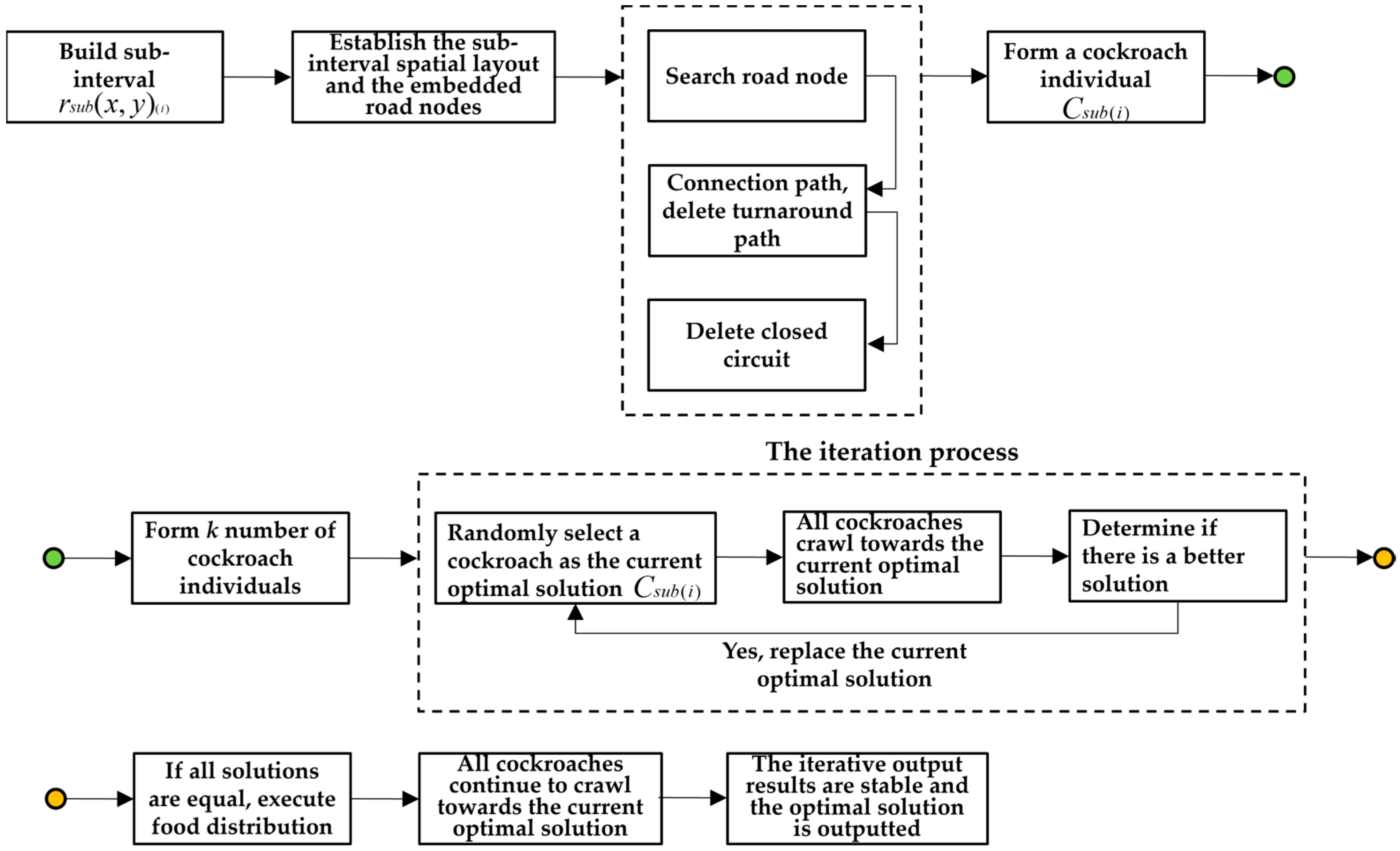
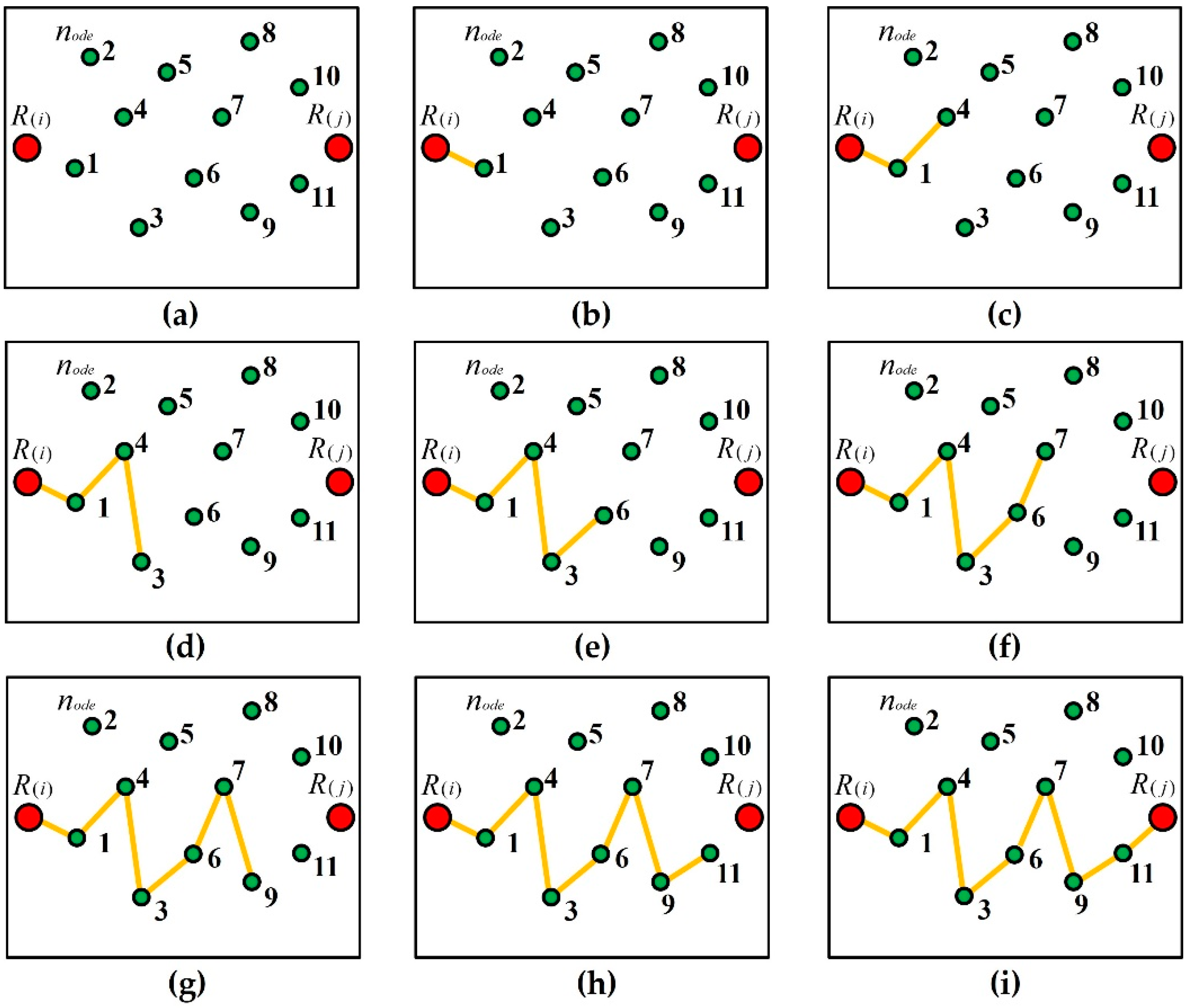
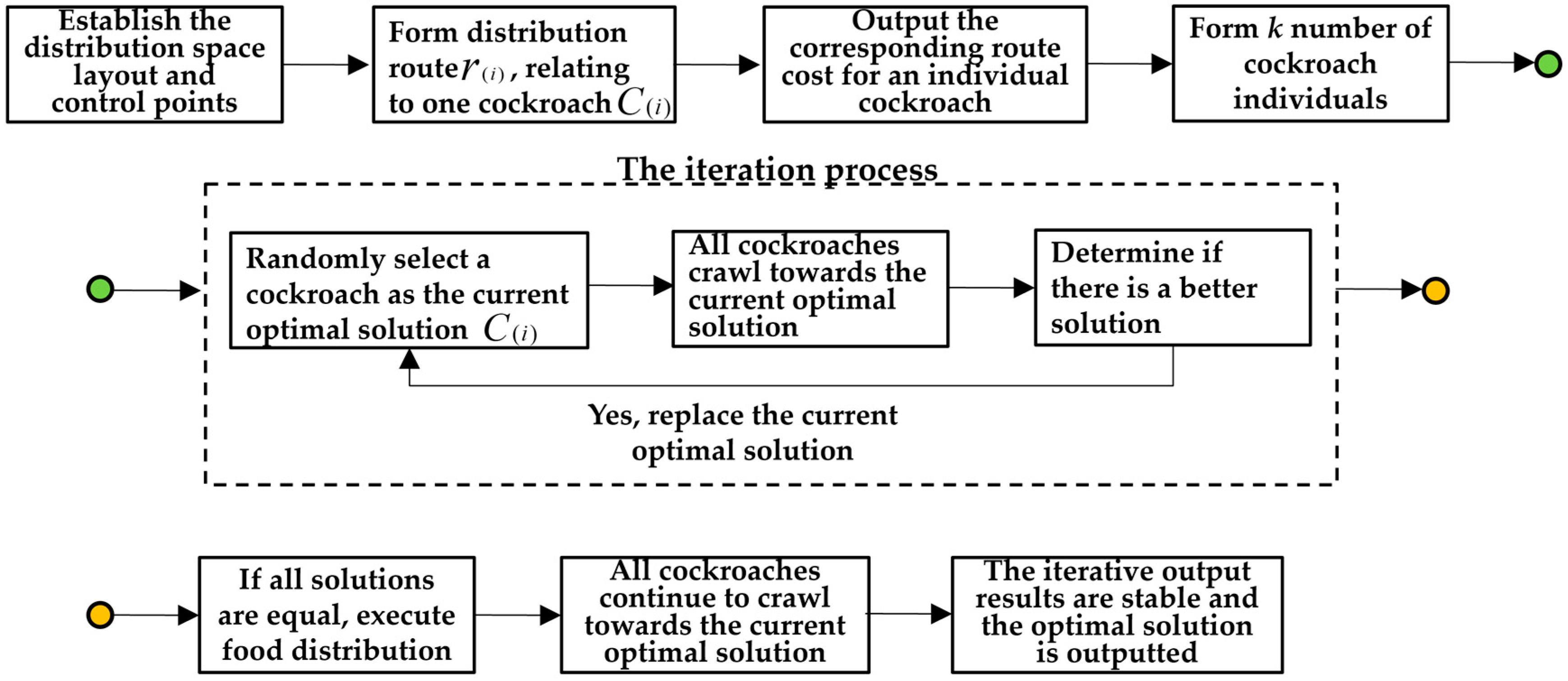
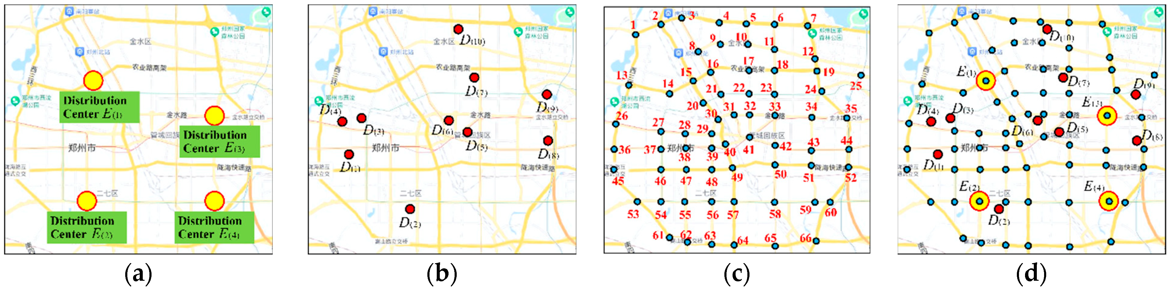
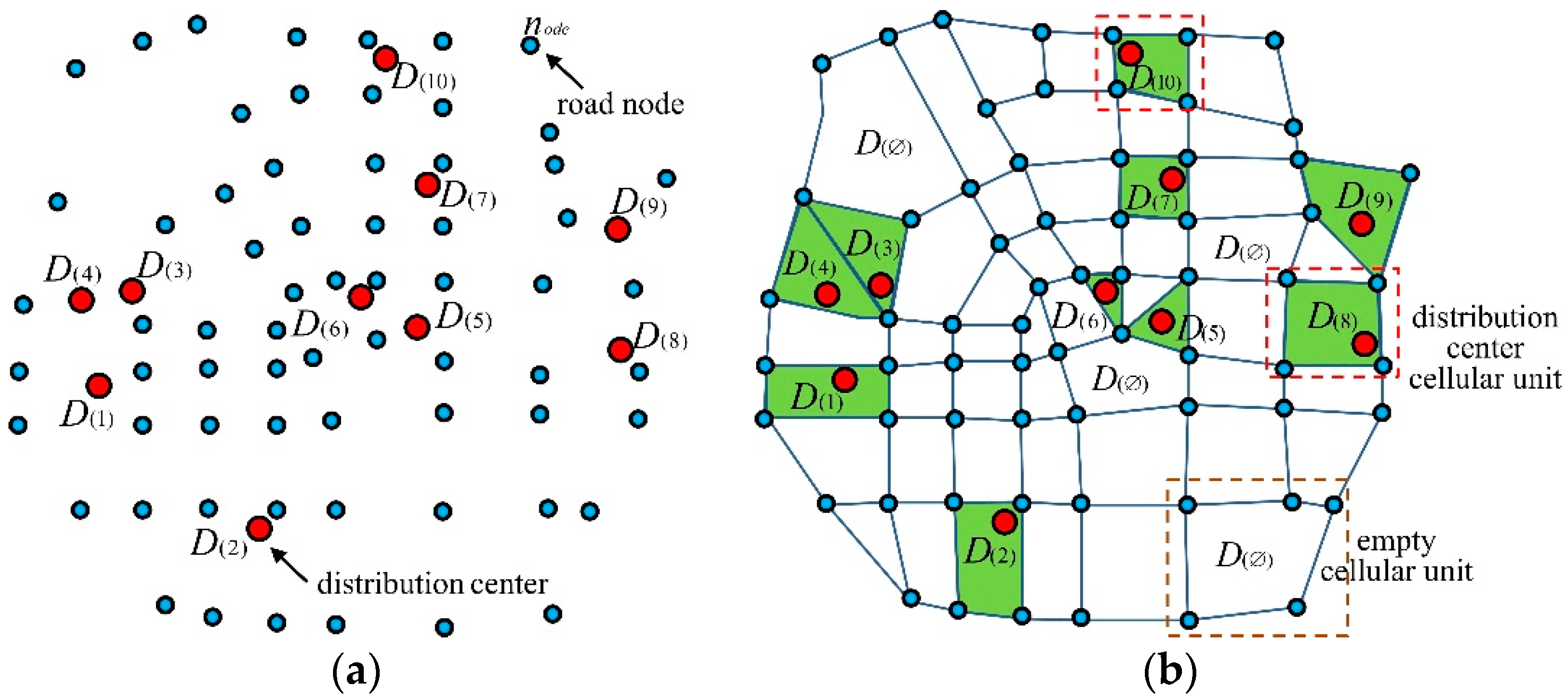
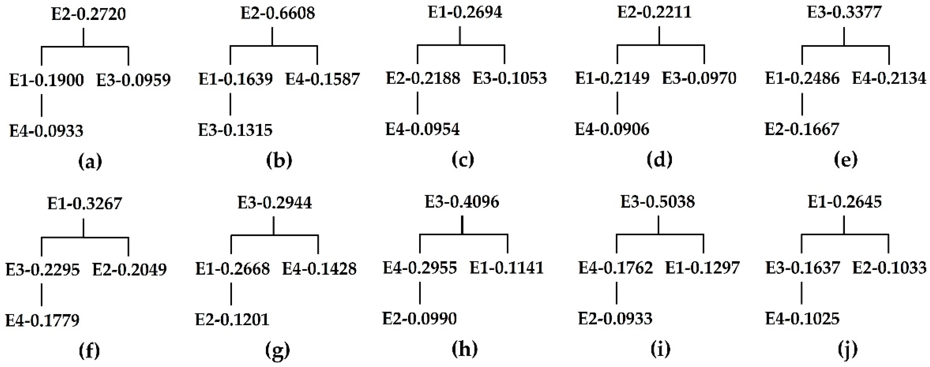
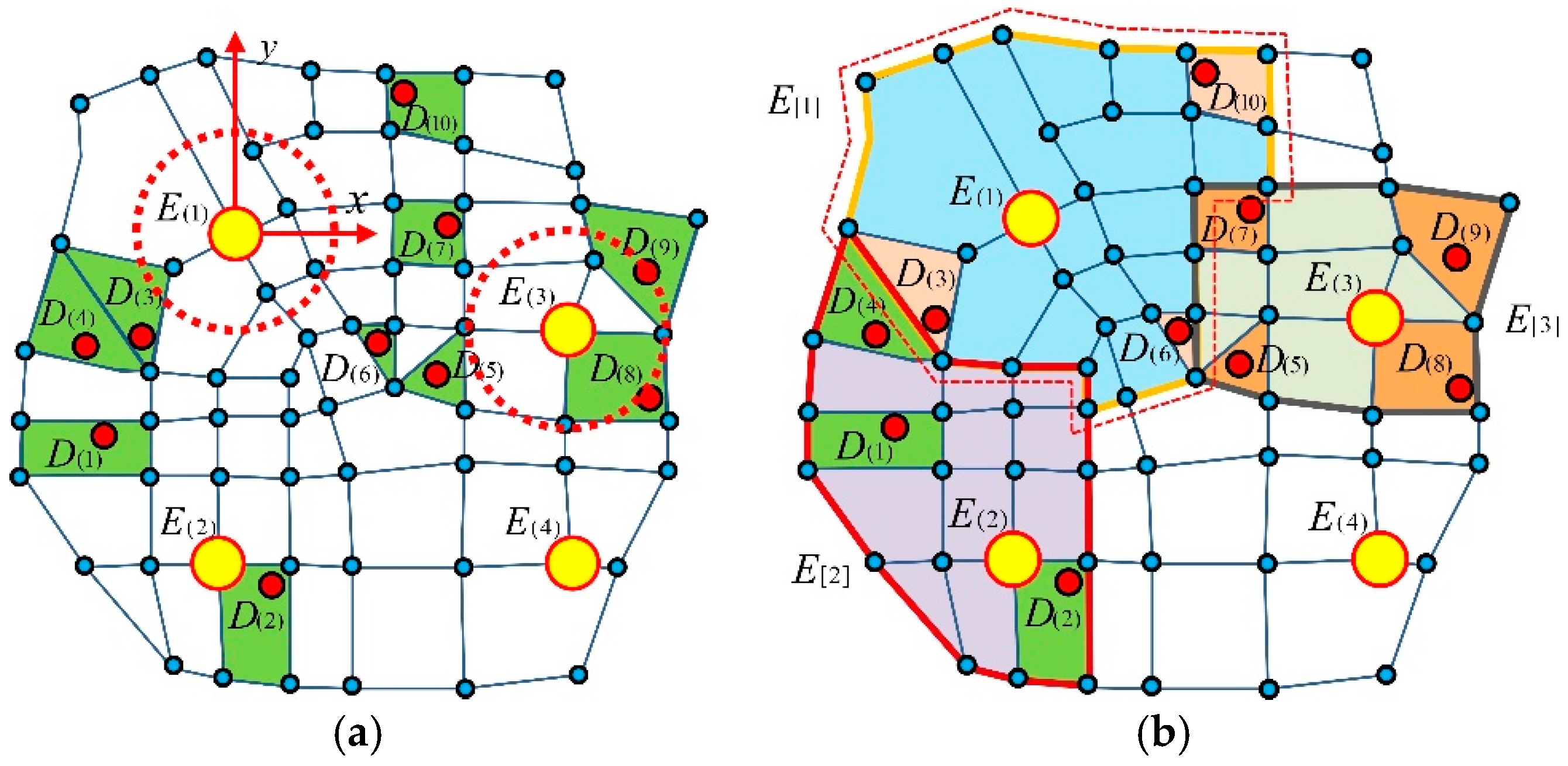
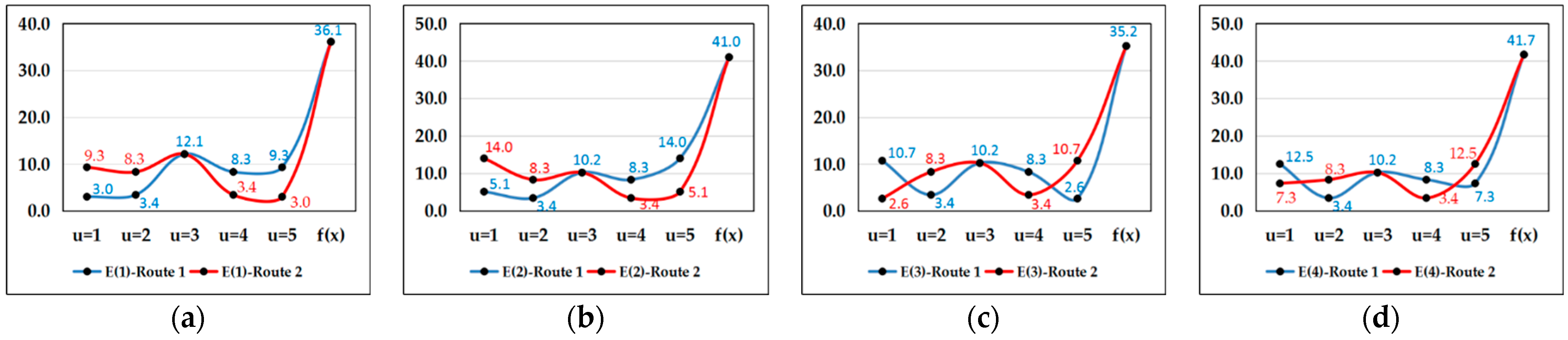
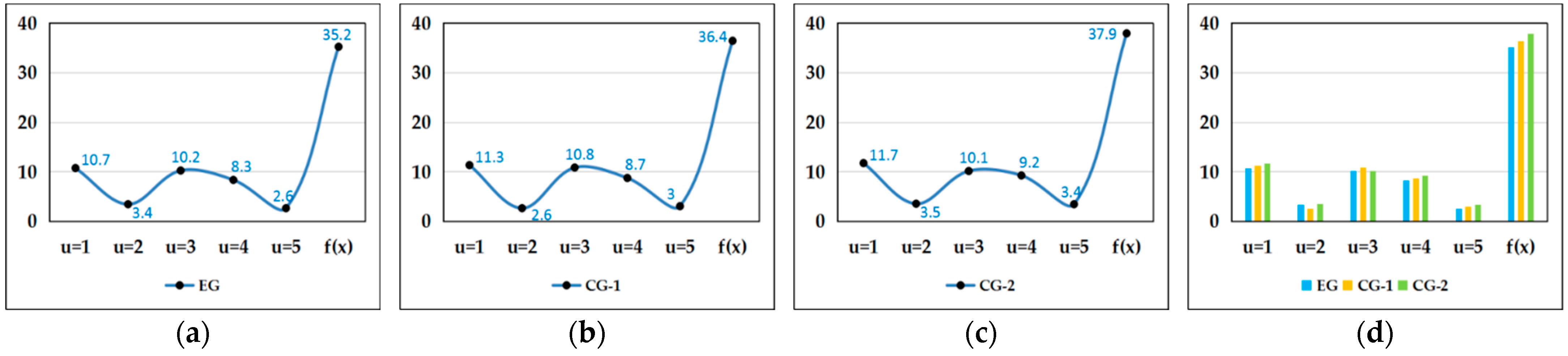
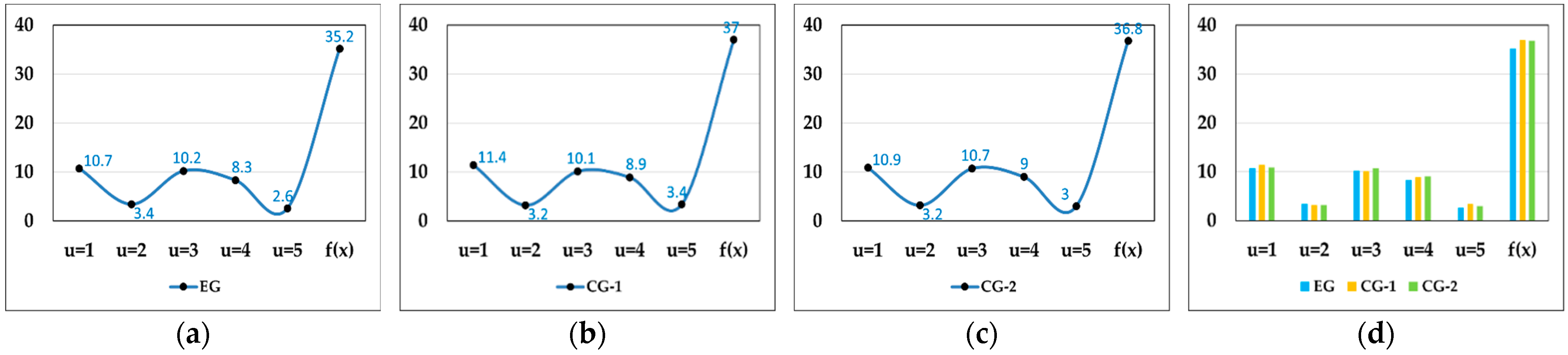
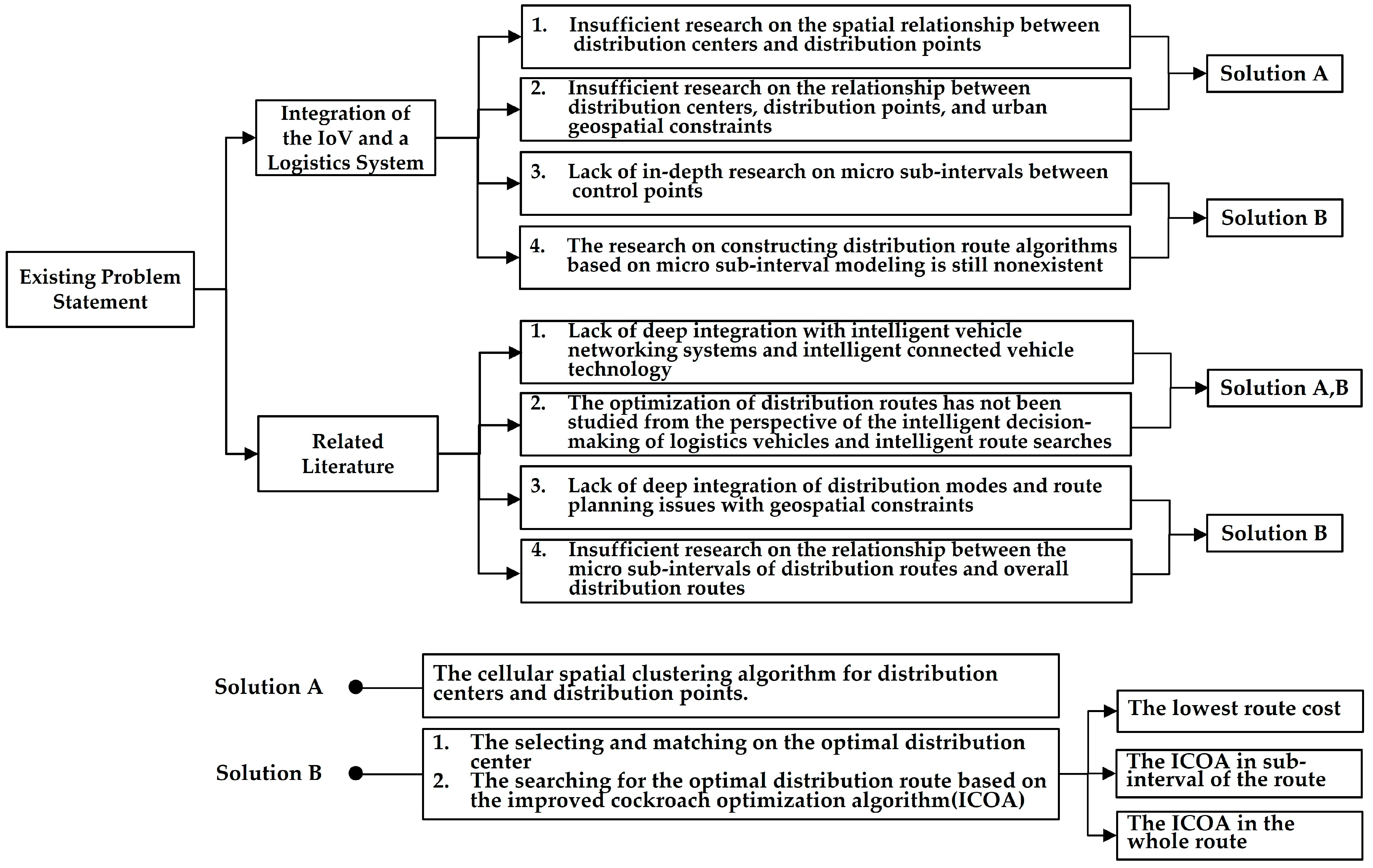
Disclaimer/Publisher’s Note: The statements, opinions and data contained in all publications are solely those of the individual author(s) and contributor(s) and not of MDPI and/or the editor(s). MDPI and/or the editor(s) disclaim responsibility for any injury to people or property resulting from any ideas, methods, instructions or products referred to in the content. |
© 2024 by the authors. Licensee MDPI, Basel, Switzerland. This article is an open access article distributed under the terms and conditions of the Creative Commons Attribution (CC BY) license (https://creativecommons.org/licenses/by/4.0/).