Article

On New Symmetric Fractional Discrete-Time Systems: Chaos, Complexity, and Control

by
Ma’mon Abu Hammad
1,
Louiza Diabi
2,*,
Amer Dababneh
1,
Amjed Zraiqat
1,
Shaher Momani
3,4,
Adel Ouannas
5 and
Amel Hioual
5,*
1
Department of Mathematics, Al-Zaytoonah University of Jordan, Amman 11733, Jordan
2
Laboratory of Dynamical Systems and Control, University of Larbi Ben M’hidi, Oum El Bouaghi 04000, Algeria
3
Nonlinear Dynamics Research Center (NDRC), Ajman University, Ajman 346, United Arab Emirates
4
Department of Mathematics, Faculty of Science, The University of Jordan, Amman 11942, Jordan
5
Department of Mathematics and Computer Sciences, University of Larbi Ben M’hidi, Oum El Bouaghi 04000, Algeria
*
Authors to whom correspondence should be addressed.
Symmetry 2024, 16(7), 840; https://doi.org/10.3390/sym16070840
Submission received: 22 May 2024 / Revised: 13 June 2024 / Accepted: 17 June 2024 / Published: 3 July 2024
(This article belongs to the Special Issue Nonlinear Symmetric Systems and Chaotic Systems in Engineering)

Abstract

:
This paper introduces a new symmetric fractional-order discrete system. The dynamics and symmetry of the suggested model are studied under two initial conditions, mainly a comparison of the commensurate order and incommensurate order maps, which highlights their effect on symmetry-breaking bifurcations. In addition, a theoretical analysis examines the stability of the zero equilibrium point. It proves that the map generates typical nonlinear features, including chaos, which is confirmed numerically: phase attractors are plotted in a two-dimensional (2D) and three-dimensional (3D) space, bifurcation diagrams are drawn with variations in the derivative fractional values and in the system parameters, and we calculate the Maximum Lyapunov Exponents (MLEs) associated with the bifurcation diagram. Additionally, we use the C 0 algorithm and entropy approach to measure the complexity of the chaotic symmetric fractional map. Finally, nonlinear 3D controllers are revealed to stabilize the symmetric fractional order map’s states in commensurate and incommensurate cases.

1. Introduction

A sine function is a mathematical formula that describes a repeating wave, which can be either a sine or cosine function adapted to characterize the periodic patterns found in real phenomena including ocean waves, light and sound waves, and others. Its applications span diverse fields in mathematics [1,2], physics [3], encryption [4], and many other fields. In recent years, researchers have been giving attention to the study of systems with sin functions [5,6]. The nonlinear sine function is handy for describing systems that vary periodically in time or space. Additionally, chaotic theory presents several significant advantages in discrete-time sine models in terms of analyzing and understanding complex maps’ behavior, which means small perturbations to the initial conditions change the future evolution of the map [7].
In general, symmetry sin maps have received more attention as they are helpful in modeling and studying phenomena that exhibit periodic and chaotic behavior [8]. They even make it possible to visualize and analyze the complex dynamics of systems that alternate between stable and unstable states. Symmetry maps are an advantageous tool in the study of nonlinear and chaotic systems, and they continue to be an active topic of research to discover new applications and understand complex dynamics [9]. Some manuscripts have been published on this discussion point at present. For instance, the control symmetry of stochastic discrete ecosystems was analyzed in [10]. Andrianov et al. [11] describe the transition from a continuous to a discrete system by changing the symmetry. In [12], propose a novel multi-stable sinusoidal map using numerical techniques. Leutcho et al. [13] investigate the chaos mechanism of the snap system both in the symmetric and non-symmetric versions. In [14], Erkan et al. explored the hyperchaotic nature of the 2D Rosenbrock map using the Rosenbrock function.
Over the last decade, discrete fractional calculus has surfaced as a enthralling research topic that has aroused interest in various fields, including mathematics. Moreover, discrete systems with fractional derivatives have obtained less attention than continuous-time systems with fractional derivatives. In order to study and work using discrete fractional calculus, new mathematical tools and techniques must be developed. Researchers have proposed several discrete difference operators, specifically the Caputo-like operator, for studying chaotic behavior in nonlinear maps and representing numerous theoretical findings of stability. In [15], the authors presented the first study of fractional chaotic maps based on the Caputo-like operator and analyzed their behavior dynamics. Furthermore, discrete dynamical systems introduced with fractional difference equations are an attractive subject that is related to several fields, such as encryption [16] and chemistry [17]. Generally, there is great interest from researchers to study discrete chaotic systems with commensurate and incommensurate fractional order [18,19]. Therefore, they are not just sensitive to the initial conditions or disorder of the systems’ factors but also to changes in the fractional orders. Additionally, it is necessary that we discuss the stabilization and synchronization of chaotic maps while analyzing their characteristics and applications.
Recently, earlier discrete systems-based sine function research has concentrated chiefly on integer-order derivatives. In contrast, the study of fractional sin maps has scant studies focused on analyzing their dynamics. In [20], Gasri and Ouannas et al. analyzed the behavior of two fractional sine maps using Caputo-type fractional maps, whereas new symmetric two-dimensional chaotic maps were analyzed in [21]. Liu et al. [22] explored the dynamics of a fractional 2D sinusoidal map and described the symmetry-breaking bifurcations of the map, while the chaotic nature of a one-dimensional map and its application in encryption was studied in [23]. Danca et al. studied symmetry-broken attractors based on Caputo’s fractional order in [24]. The main discoveries and findings of this paper are summarized as follows:
  • A new symmetric fractional map with a sine function and complex nonlinear chaotic behavior is explored in two cases, commensurate order and incommensurate order, through numerical techniques.
  • Preliminaries of discrete fractional calculus and a description of a new symmetric fractional-order map add to the analysis of the stability of equilibrium points.
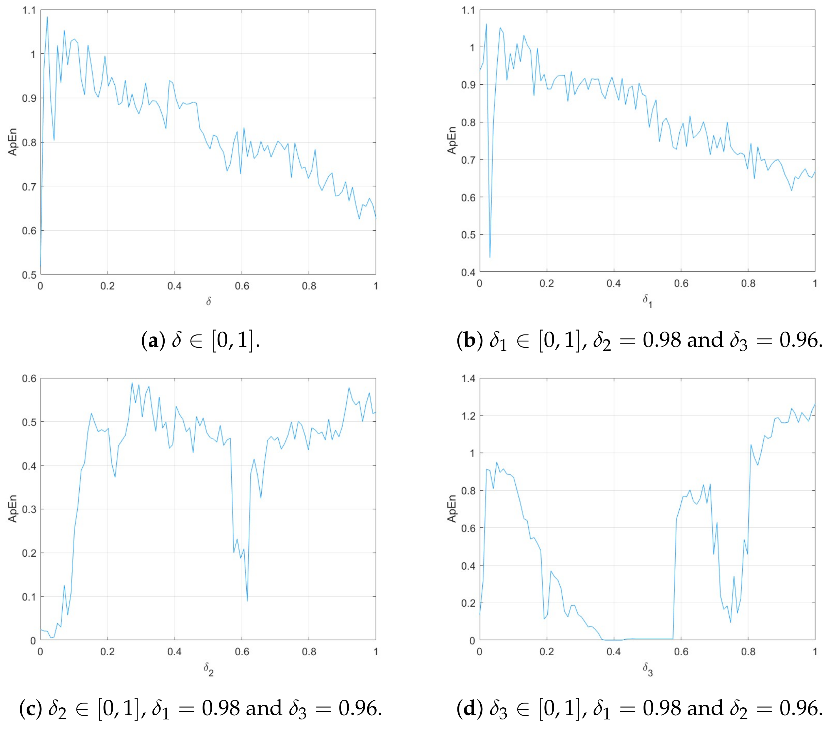
  • We give the approximate entropy (ApEn) and C 0 complexity for evaluating the complexity of chaos in the new symmetric fractional map in two cases.
  • Stabilization of the symmetric fractional map is attained resting on the stability theorems of linear maps.
The remaining is explained as follows: in Section 2, we give the necessary preliminary notions of discrete fractional calculus and establish the Caputo-like fractional discrete version of the symmetric map. In Section 3, the model’s symmetric map and the stability analysis of its equilibrium points are investigated under the commensurate fractional order. In Section 4, we provide an evaluation and analysis of the symmetric incommensurate map case. Section 5 entails the C 0 complexity and the entropy approach (ApEn) for the statistical complexity of chaos. In Section 6, nonlinear controllers are intended to stabilize the symmetric fractional map in both commensurate and incommensurate cases. This article concludes by discussing the most important results obtained throughout the work in Section 7.

2. Model Description and Basic Tools

2.1. Basic Tools

The present paper aims to describe our symmetric fractional map based on the δ -th Caputo-like difference operator   c Δ η δ , described as [25]
  c Δ η δ φ ( r ) = Δ η ( δ ) Δ φ ϖ ,
where ϖ N η + δ , 1 < δ and = δ + 1 . The fractional sum   c Δ η δ is characterized as [26]
  c Δ η δ φ ( r ) = 1 Γ δ ϖ = δ r δ r 1 ϖ δ 1 φ ϖ .
The following theorem is used to obtain the numerical formula of the symmetric fractional map:
Theorem 1
([15]). The solution of the following fractional system,
  c Δ η δ φ ( r ) = h ( r + δ 1 , φ ( r 1 + δ ) ) Δ j φ ( η ) = φ j , = δ + 1
is expressed by
φ ( r ) = φ 0 ( r ) + 1 Γ ( δ ) ϖ = η + δ r δ ( r 1 ϖ ) ( δ 1 ) h ( ϖ + δ 1 , φ ( ϖ + δ 1 ) ) ,
where φ 0 ( r ) = j = 0 1 ( r η ) j Γ ( j + 1 ) Δ j φ ( 0 ) .
For η = 0 , = 1 , j = ϖ + δ 1 , and ( r 1 ϖ ) ( δ 1 ) = Γ ( r ϖ ) Γ ( r ϖ δ + 1 ) , the numerical expression (4) for δ ( 0 , 1 ] can be obtained via
φ ( r ) = φ ( 0 ) + 1 Γ ( δ ) j = 0 r 1 Γ ( r 1 + δ j ) Γ ( r j ) h ( j , φ ( j ) ) .
The next theorems are practiced to value the stability of the equilibrium point for nonlinear discrete fractional systems under commensurate and incommensurate orders.
Theorem 2
([27]). Consider the linear discrete commensurate system
  C Δ η δ φ ( r ) = A φ ( r 1 + δ ) , r N η + 1 δ ,
where φ ( r ) = ( φ 1 ( r ) , . . . , φ n ( r ) ) T and 0 < δ < 1 . Let λ ι be the eigenvalues of the matrix A R n × n . If all λ ι satisfy
λ ι ν C : | ν | 2 cos | a r g ν | π 2 δ δ a n d | a r g ν | δ π 2 ,
then the zero equilibrium of (6) is asymptotically stable.
Theorem 3
([28]). Consider the following system:
  c Δ η δ 1 z 1 ( r ) = ϑ 1 ( z ( r 1 + δ 1 ) ) ,   c Δ η δ 2 z 2 ( r ) = ϑ 2 ( z ( r 1 + δ 2 ) ) , r = 0 , 1 , ,   c Δ η δ n z n ( r ) = ϑ n ( z ( r 1 + δ n ) ) .
Let z ( r ) = ( z 1 ( r ) , . . . , z n ( r ) ) T R n , ϑ = ( ϑ 1 , . . . , ϑ n ) : R n R n , and set M to be the (LCM) of the denominators v ¯ ι of δ ι , where δ ι ( 0 , 1 ] , added to δ ι = w ¯ ι v ¯ ι , ( w ¯ ι , v ¯ ι ) = 1 , w ¯ ι , v ¯ ι Z + , ι = 1 , . . . , n .
If all roots of (9),
d e t ( d i a g ( λ M δ 1 , , λ M δ n ) ( 1 λ M ) A ) = 0 ,
are included in C / K τ , where
K τ = { ω C : | ω | 2 cos | a r g ω | τ τ a n d | a r g ω | ϖ π 2 } ,
with τ = 1 M and where A is the Jacobin matrix of (8), then the zero solution is locally asymptotically stable.

2.2. Description of the Fractional Map

Very recently, the addition of a sine function to discrete symmetry maps has created rich dynamics of models [29,30]. In this work, we offer a thorough analysis of the new 3D symmetric fractional map, which is formulated using the Caputo-like operator   c Δ η δ as follows:
  c Δ η δ z 1 ( r ) = z 2 ( ξ ) z 1 ( ξ )   c Δ η δ z 2 ( r ) = sin ( z 3 ( ξ ) ) z 2 ( ξ )   c Δ η δ z 3 ( r ) = β 1 z 1 ( ξ ) + β 2 z 2 ( ξ ) γ sin ( z 3 ( ξ ) ) z 3 ( ξ ) ,
where ξ = r 1 + δ , z 1 , z 2 , z 3 denote the state variables, and β 1 , β 2 , γ are the bifurcation parameters. In this paper, fractional map (11) is symmetric using the following transformation: G : ( z 1 , z 2 , z 3 ) ( z 1 , z 2 , z 3 ) . Therefore, each attractor of the map will emerge in a reciprocally symmetric pair.

3. The Commensurate Fractional Map

In the following, the rich dynamics of the proposed symmetric fractional map, (11), will be studied in a commensurate case.

3.1. Stability Analysis

In this subsection, the stability of the zero equilibrium point of map (11) is analyzed. To calculate the equilibrium points, solving the equations below:
z 2 z 1 = 0 sin ( z 3 ) z 2 = 0 β 1 z 1 + β 2 z 2 γ sin ( z 3 ) z 3 = 0 .
With a simple computation, we obtain z 3 ( β 1 + β 2 γ ) sin ( z 3 ) = 0 . Clearly, the map has an equilibrium point ( 0 , 0 , 0 ) . In the context of the symmetric fractional discrete-time system discussed in our paper, instability at the origin can signal the emergence of chaotic behavior and complex dynamics. This approach helps us understand how minor perturbations near the origin can cause substantial and unpredictable changes in the system’s trajectory. Thus, it forms the basis for exploring the model’s chaos, complexity, and control characteristics.
Proposition 1.
The ( 0 , 0 , 0 ) equilibrium point of system (11) is unstable for all δ due to
λ ι > 2 cos | a r g λ ι | π 2 δ δ , ι = 1 , 2 , 3 .
Proof. 
In order to analyze the stability of symmetric map (11) according to Theorem 2 and to prove the existence of chaos, we calculate the Jacobian matrix J ι of the map evaluated at ( 0 , 0 , 0 ) as follows:
J ι = 1 1 0 0 1 1 β 1 β 2 γ 1 .
Take the parameters of the map, β 1 = 1.7 , β 2 = 1.9 , and γ = 0.5 , and find the eigenvalues of the matrix J ι . The associated characteristic equation is defined by
λ 3 3.5 λ 2 2.1 λ + 2.1 = 0 .
Equation (14) has three eigenvalues, λ 1 = 2.00391 + 0.345847 i , λ 2 = 2.00391 0.345847 i , and λ 3 = 0.507826 , and let us consider δ = 0.8 . Based on Theorem 2, the asymptotic conditions for the stability of the equilibrium point are not verified due to
λ ι > 2 cos | a r g λ ι | π 2 0.8 0.8 , ι = 1 , 2 , 3 .
Hence, the symmetric fractional map in (11) satisfies the necessary condition for us to present chaos. □

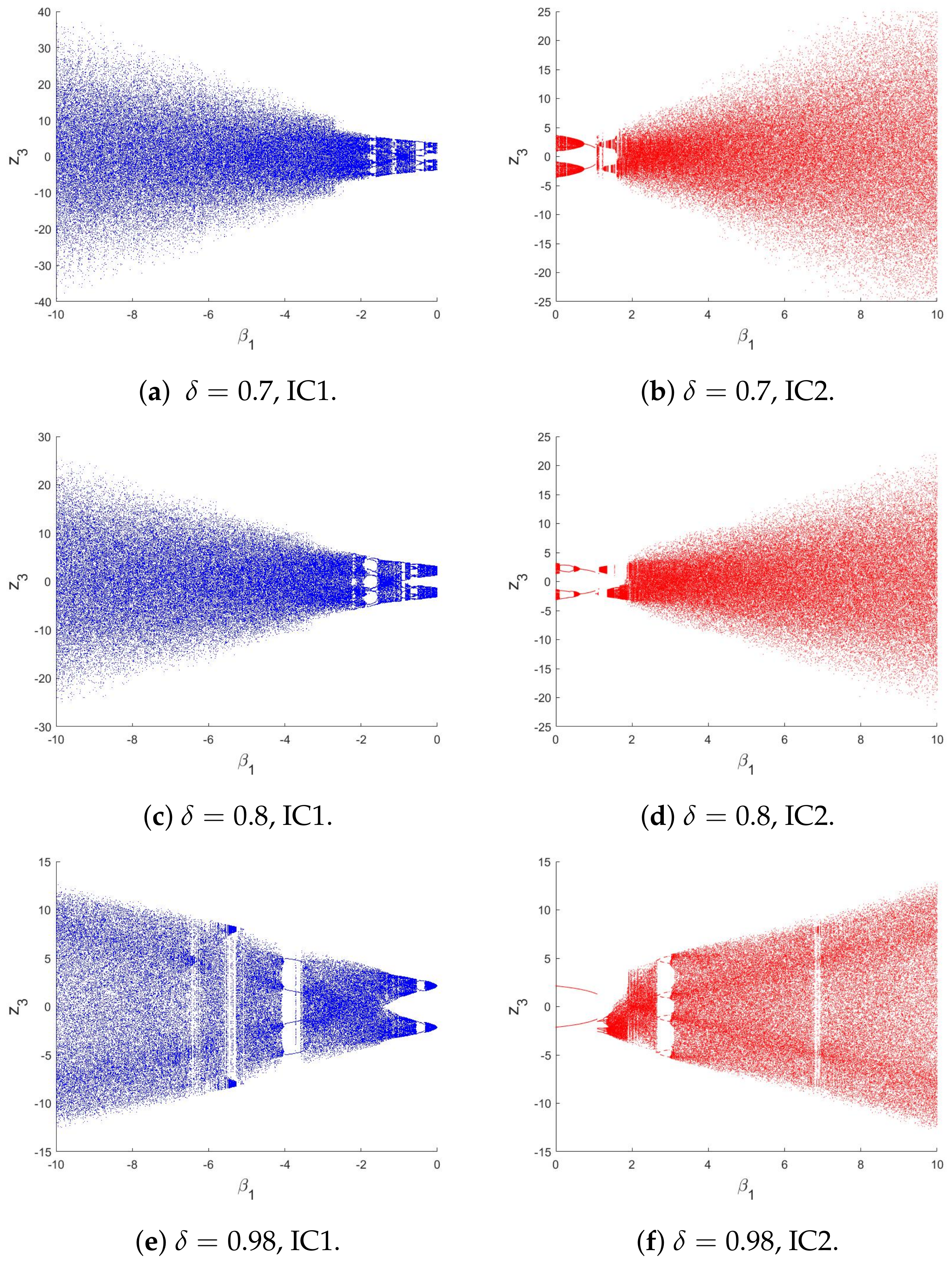
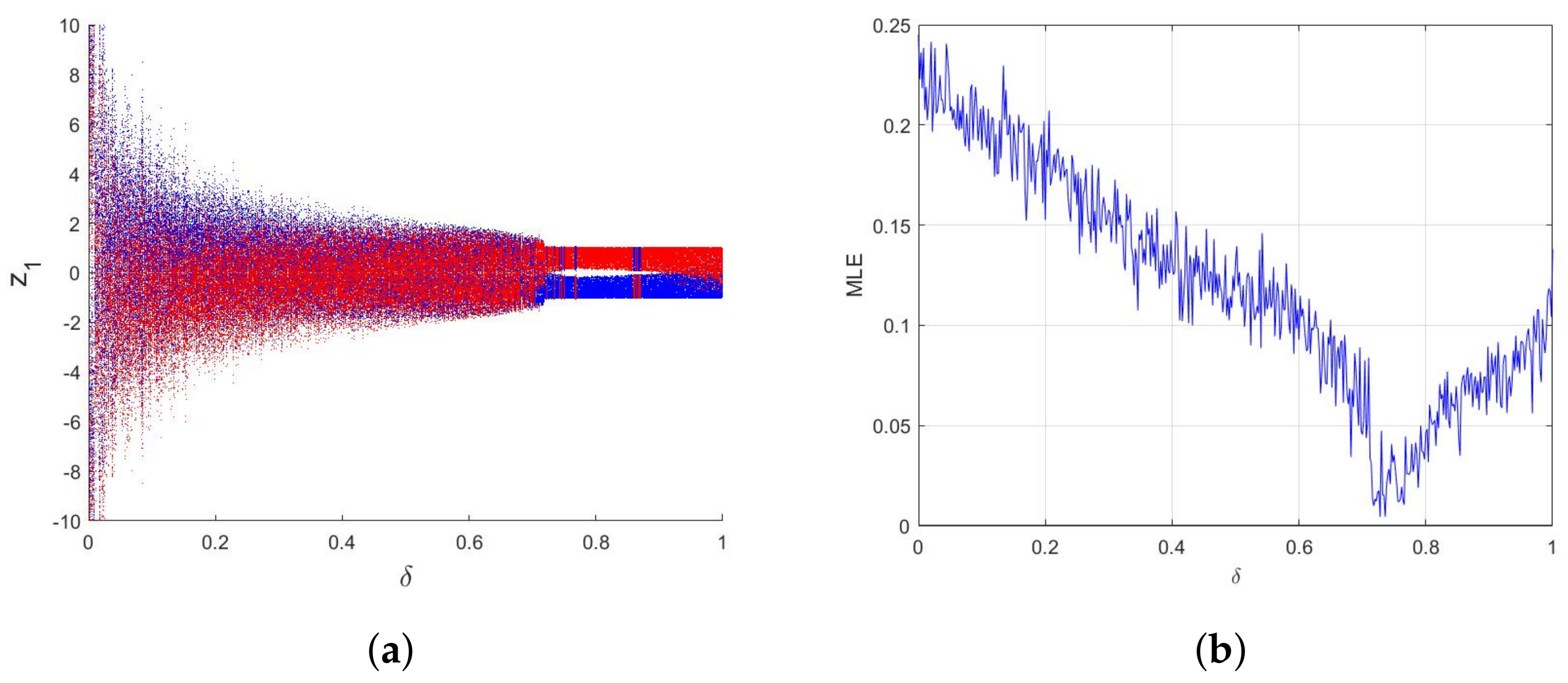
3.2. Dynamic Analysis

To evaluate the influence of the equal fractional order δ on the dynamics of the symmetric fractional map in (11), we utilize bifurcation diagrams and Maximum Lyapunov Exponent (MLE) calculations for various fractional values of δ , while varying the parameter β 1 over [ 10 , 10 ] . These results are depicted in Figure 1 and Figure 2 for two distinct initial conditions: IC1 = ( 0.8 , 2 , 0 ) (blue) and IC2 = ( 0.8 , 2 , 0 ) (red).
Firstly, in accordance with Theorem 1, we derive the numerical formulation of symmetric commensurate map (11):
z 1 ( r ) = z 1 ( 0 ) + j = 0 r 1 Γ ( δ j 1 + r ) Γ ( δ ) Γ ( r j ) z 2 ( j ) z 1 ( j ) z 2 ( r ) = z 2 ( 0 ) + j = 0 r 1 Γ ( δ j 1 + r ) Γ ( δ ) Γ ( r j ) sin ( z 3 ( j ) ) z 2 ( j ) z 3 ( r ) = z 3 ( 0 ) + j = 0 r 1 Γ ( δ j 1 + r ) Γ ( δ ) Γ ( r j ) β 1 z 1 ( j ) + β 2 z 2 ( j ) γ sin ( z 3 ( j ) ) z 3 ( j ) .
To delve into the dynamics of the symmetric commensurate map given in (11) regarding the fractional order δ , take the two initial conditions IC1 (blue) and IC2 (red) and the system’s parameters as β 1 = 1.7 , β 2 = 1.9 , and γ = 0.5 . The bifurcation diagram of map (11) when β 1 varies at [ 10 , 0 ] for IC1 and at [ 0 , 10 ] for IC2 with various δ values is shown in Figure 1. We notice that when δ = 0.7 and δ = 0.8 the map exhibits irregular movements, changing between chaotic with period-doubling bifurcation and periodic at 1.7 < β 1 < 1.7 ; we conclude that the map has the symmetry-breaking bifurcation, which confirms the sensitivity of the map to the initial condition and the commensurate derivative. From Figure 1a,c the map is totally chaotic at β 1 [ 10 , 1.7 ] while in Figure 1b,d it becomes chaotic at the interval β 1 [ 1.7 , 10 ] . However, for δ = 0.98 the symmetric commensurate map in (11) displays multiple movements, including non-chaotic and chaotic regions. We observe the typical symmetry breaking of the map as shown in Figure 1e,f.
We calculate the Maximum Lyapunov Exponents of the fractional system using the Jacobin matrix algorithm [31], which allows us to understand the fundamental aspect of chaos theory in the symmetric fractional map. The tangent map J is defined by
J = k 1 ( ) k 2 ( ) k 3 ( ) R 1 ( ) R 2 ( ) R 3 ( ) W 1 ( ) W 2 ( ) W 3 ( ) ,
where
K i ( ) = K i ( 0 ) + 1 Γ ( δ ) j = 0 1 Γ ( δ + j 1 ) Γ ( j ) ( R i ( j ) K i ( j ) ) R i ( ) = R i ( 0 ) + 1 Γ ( δ ) j = 0 1 Γ ( δ + j 1 ) Γ ( j ) ( W i ( j ) cos ( z 3 ( j ) ) R i ( j ) ) , i = 1 , 2 , 3 , W i ( ) = W i ( 0 ) + 1 Γ ( δ ) j = 0 1 Γ ( δ + j 1 ) Γ ( j ) ( β 1 K i ( j ) + β 2 R i ( j ) γ W i ( j ) cos ( z 3 ( j ) ) W i ( j ) ) ,
where
K 1 ( 0 ) K 2 ( 0 ) K 3 ( 0 ) R 1 ( 0 ) R 2 ( 0 ) R 3 ( 0 ) W 1 ( 0 ) W 2 ( 0 ) W 3 ( 0 ) = 1 0 0 0 1 0 0 0 1 .
Then, the L E ϖ of the fractional map can be given by
L E ϖ = lim 1 ln | λ ϖ ( ) | , for ϖ = 1 , 2 , 3 ,
where λ ϖ ( ) are the eigenvalues of J .
Furthermore, Figure 2 illustrates the MLE of the symmetric commensurate map in (11), which is calculated using MATLAB R2024a script, which confirms the results obtained from the bifurcation shown Figure 1. Note that the MLE values are negative, indicating non-chaotic behavior. Conversely, the map exhibits a chaotic region when the MLE values are positive.
Next, to provide further clarity on the behavior of (11), Figure 3 illustrates the bifurcation diagram and the associated Maximum Lyapunov Exponent (MLE) of the symmetric commensurate map in (11) across the range of fractional order δ from 0 to 1. The plot considers two initial conditions, IC1 (blue) and IC2 (red), with parameters set to β 1 = 1.7 , β 2 = 1.9 , and γ = 0.5 .
The map initially exhibits chaotic behavior, as indicated by the bifurcation diagram and MLE. However, as the fractional order δ increases, the map transitions away from chaos. With further increases in δ , the symmetric commensurate map in (11) returns to a state where both its symmetry and chaotic properties are evident.
For completeness, to further provide clarity on the dynamic characteristics of the map, Figure 4 simulates the evolution of the states z 1 , z 2 , and z 3 for the proposed symmetric commensurate map in (11) when δ = 0.8 , while Figure 5 depicts the map exhibiting different chaotic attractors in 2D and 3D space with IC1 (blue), IC2 (red) for ( δ = 0.01 , 0.7 , 0.78 , 0.8 , 0.98 ) , and δ = 1 ; note that when δ = 1 , the symmetric commensurate map in (11) refers to the integer-order map.

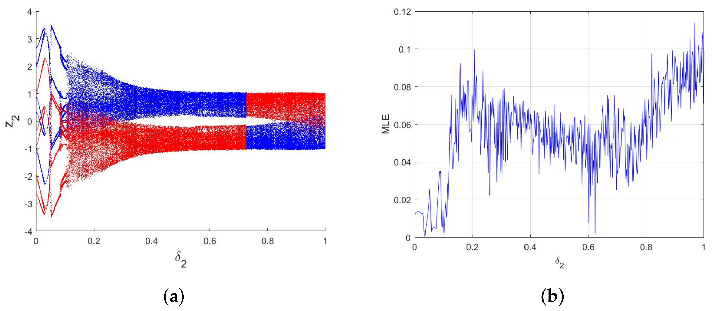
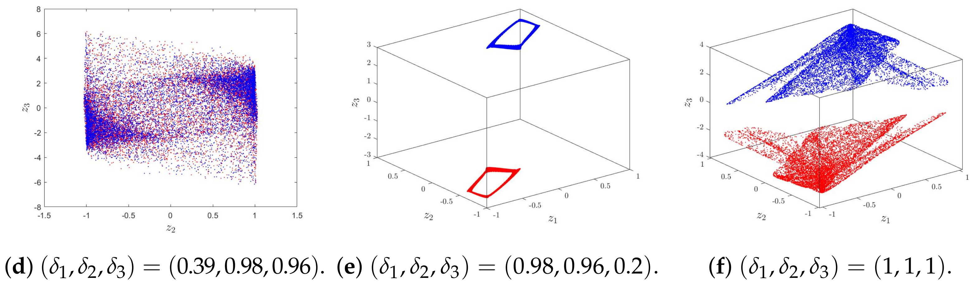
4. The Incommensurate Fractional System

With the aim of examining the impact of the incommensurate fractional values ( δ 1 , δ 2 , δ 3 ) and β 1 (the system factor) on the behaviors of the proposed symmetric fractional map in (20) using bifurcation and the associated MLE, the representation of the new 3D symmetric incommensurate order map is as follows:
  c Δ η δ 1 z 1 ( r ) = z 2 ( ξ 1 ) z 1 ( ξ 1 )   c Δ η δ 2 z 2 ( r ) = sin ( z 3 ( ξ 2 ) ) z 2 ( ξ 2 )   c Δ η δ 3 z 3 ( r ) = β 1 z 1 ( ξ 3 ) + β 2 z 2 ( ξ 3 ) γ sin ( z 3 ( ξ 3 ) ) z 3 ( ξ 3 ) ,
where ξ 1 = r 1 + δ 1 , ξ 2 = r 1 + δ 2 , and ξ 3 = r 1 + δ 3 .

4.1. Equilibrium Stability

Now, we analyze the stability of the equilibrium point of map (20) according to Theorem 3 and prove the existence of chaos:
Proposition 2.
The ( 0 , 0 , 0 ) equilibrium point of system (20) is unstable if there is an eigenvalue λ ι satisfying λ ι K 1 M for β 1 = 1.9 , β 2 = 1.7 , and γ = 0.5 .
Proof. 
Take ( δ 1 , δ 2 , δ 3 ) = ( 0.7 , 0.98 , 0.96 ) . Note that M = 50 . We calculate
det λ 37 0 0 . 0 λ 49 0 0 0 λ 48 1 λ 50 1 1 0 0 1 1 1.7 1.9 1.5 = 0 ,
which is equivalent to
2.1 λ 150 + 1.5 λ 149 + λ 148 λ 147 0.4 λ 137 1.5 λ 136 λ 135 + λ 134 6.3 λ 100 3 λ 99 2 λ 98 + λ 97 + 0.8 λ 87 + 1.5 λ 86 + λ 85 + 6.3 λ 50 + 1.5 λ 49 + λ 48 0.4 λ 37 2.1 = 0 .
Then, solving Equation (21), out of λ ι , ( ι = 1 , . . . , 150 ) solutions there are λ ι = ( 1.01126 ± 0.00361356 i ) K 1 50 , which implies | arg λ ι | 2 cos 50 | arg λ ι | 1 50 and | arg λ ι | π 100 . As a result, according to Theorem 3, the equilibrium point ( 0 , 0 , 0 ) is unstable. Therefore, in this case symmetric incommensurate map (20) satisfies the necessary condition for having a chaotic attractor. □

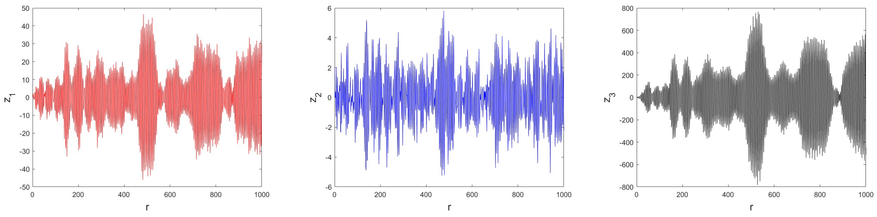
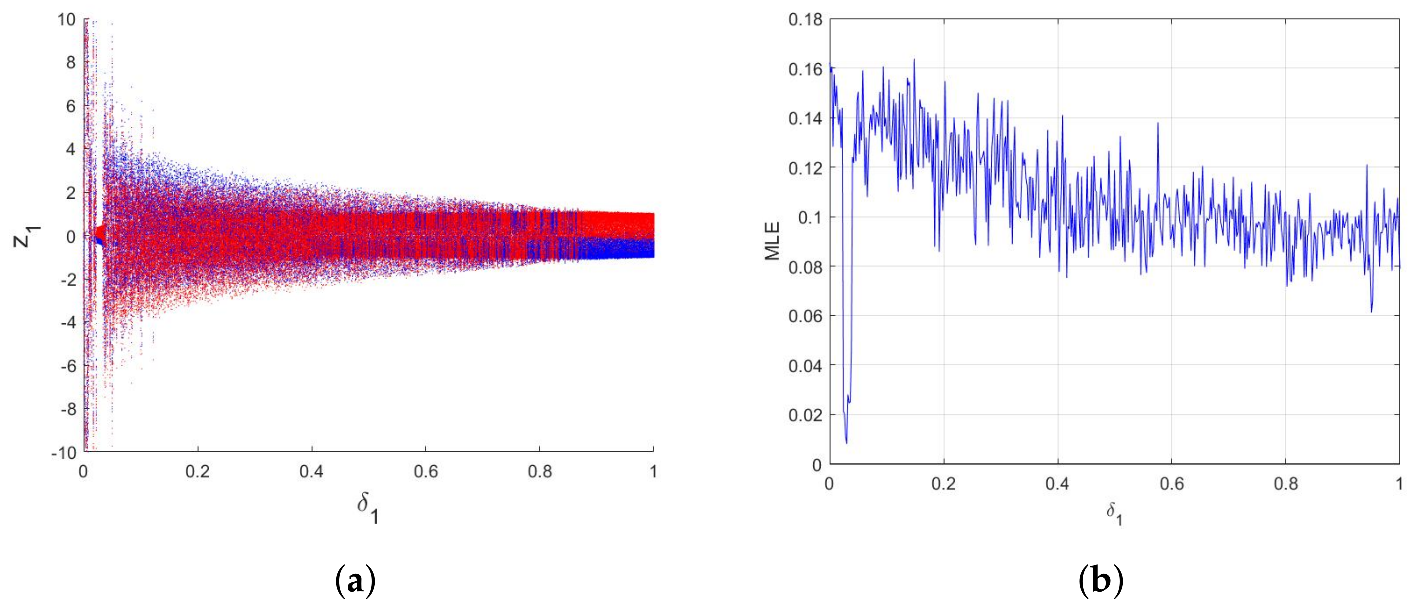
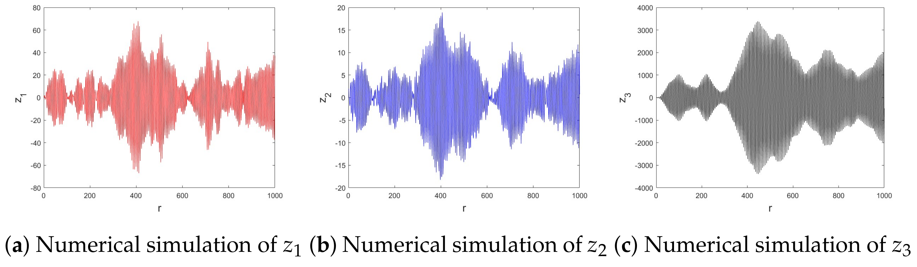
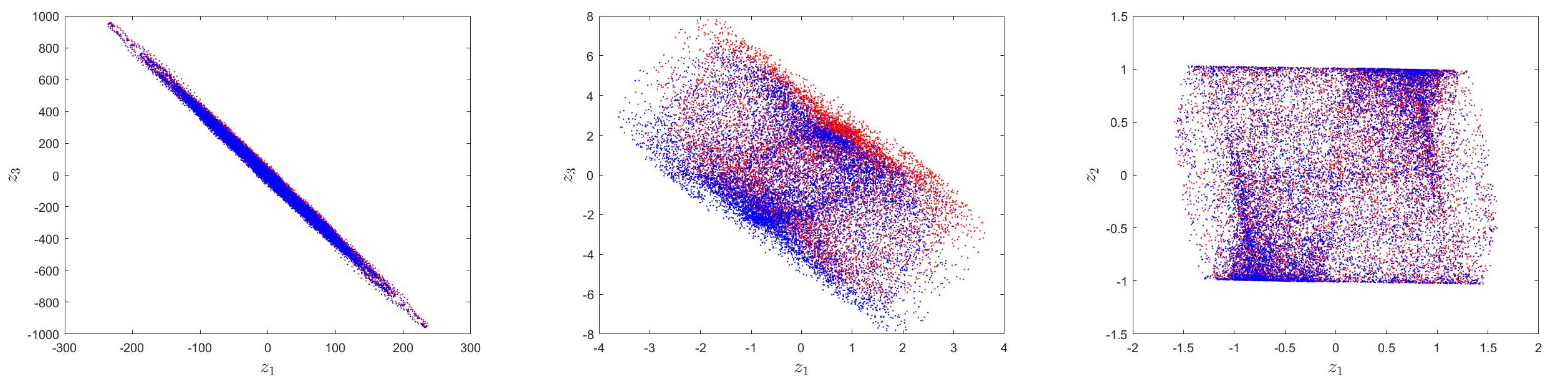
4.2. Numerical Chaos

The numerical formula of map (20) is formulated as follows:
z 1 ( r ) = z 1 ( 0 ) + j = 0 r 1 Γ ( r + δ 1 j 1 ) Γ ( δ 1 ) Γ ( r j ) z 2 ( j ) z 1 ( j ) z 2 ( r ) = z 2 ( 0 ) + j = 0 r 1 Γ ( r + δ 2 j 1 ) Γ ( δ 2 ) Γ ( r j ) sin ( z 3 ( j ) ) z 2 ( j ) z 3 ( r ) = z 3 ( 0 ) + j = 0 r 1 Γ ( r + δ 3 j 1 ) Γ ( δ 3 ) Γ ( r j ) β 1 z 1 ( j ) + β 2 z 2 ( j ) γ sin ( z 3 ( j ) ) z 3 ( j ) .
To investigate the behavior of the map described in (20) across various fractional orders ( δ 1 , δ 2 , δ 3 ) and initial conditions IC1 (blue) and IC2 (red), we present the bifurcation diagram of symmetric incommensurate map (20) in Figure 6. The diagram depicts the variation in β 1 over two ranges: [ 10 , 0 ] with IC1 and [ 0 , 10 ] with IC2 for different fractional values ( δ 1 , δ 2 , δ 3 ) .
Specifically, when ( δ 1 , δ 2 , δ 3 ) = ( 0.7 , 0.98 , 0.96 ) and ( 0.98 , 0.7 , 0.96 ) , the map exhibits periodic and chaotic behavior, including period-doubling bifurcations. Notably, within the interval β 1 ] 1.7 , 1.7 [ , the map shows symmetry-breaking behavior, highlighting its sensitivity to initial conditions and incommensurate derivatives. In contrast, for β 1 [ 10 , 1.7 ] with IC1 and β 1 [ 1.7 , 10 ] with IC2, the chaotic region widens, as shown in Figure 6a–d.
Additionally, for ( δ 1 , δ 2 , δ 3 ) = ( 0.98 , 0.7 , 0.96 ) , symmetric map (20) exhibits chaotic behavior across several intervals, as illustrated in Figure 6e,f. The Maximum Lyapunov Exponent (MLE) in Figure 7 further confirms these findings, depicting MLE values fluctuating between negative and positive, consistent with the bifurcation diagram results in Figure 6.
Next, with the goal of noting the influence of the incommensurate order, we draw the bifurcation and the associated MLE of symmetric incommensurate map (20) when the fractional δ 1 is the bifurcation parameter and we choose δ 2 = 0 , 98 and δ 3 = 0.96 . This diagram is drawn with IC1 (blue), IC2 (red), and the same parameters, β 1 = 1.7 , β 2 = 1.9 , and γ = 0.5 , as illustrated in Figure 8. We can see that the map is chaotic with different intensities at δ 1 ( 0 , 1 ] . Additionally, we evaluate the dynamics of symmetric incommensurate map (20) when the fractional order δ 2 ( 0 , 1 ] . Figure 9 displays the bifurcation and its associated MLE for δ 1 = 0.98 and δ 3 = 0.96 . Plainly, with increasing δ 2 values, we observe a shift from increases to decreases until it reaches a higher chaotic level and the MLE takes its highest values, unlike the beginning, where there is less chaotic behavior. Furthermore, in Figure 10 we chose δ 1 = 0.98 and δ 2 = 0.96 , the fractional order δ 3 was varied within the range ( 0 , 1 ] , and the trajectories were stable when 0.38 < δ 3 < 0.58 where the MLE values were negative, whereas the states of symmetric map (20) is chaotic when δ 3 takes smaller and larger values. According to these findings, the symmetry of map (20) is not impacted by increasing the incommensurate derivative orders.
Namely, Figure 11 represents the evolution of states z 1 , z 2 , and z 3 for the proposed symmetric incommensurate map (20) when ( δ 1 , δ 2 , δ 3 ) = ( 0.7 , 0.98 , 0.96 ) , whereas Figure 12 illustrates the phase attractors via distinct incommensurate orders ( δ 1 , δ 2 , δ 3 ) with IC1 (blue) and IC2 (red) in 2D and 3D planes.

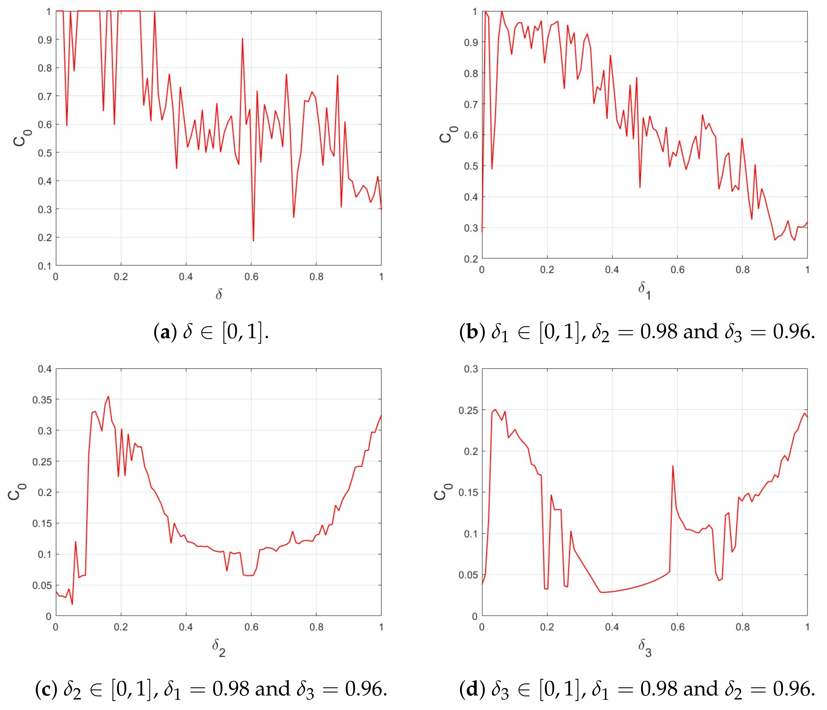
5. Chaotic Complexity

Understanding the degree of chaos is crucial for analyzing the dynamics of complex systems. In this section, we investigate the chaotic complexity of the symmetric fractional map in two distinct scenarios: commensurate orders, described by Equation (11), and incommensurate orders, described by Equation (20). By examining these cases, we aim to provide a comprehensive analysis of how different fractional orders impact the behavior of the system. We will employ various metrics and methods to quantify the level of chaos and demonstrate the resulting dynamical phenomena. This investigation will help in understanding the underlying mechanisms that drive chaotic behavior in symmetric fractional maps.

5.1. C 0 Complexity

In this part, we compute the complexity of the symmetric fractional map via commensurate order (11) and incommensurate order (20) by way of the C 0 complexity method [32], which is derived from the inverse Fourier transform:
For { φ ( α ) , α = 1 , . . , D 1 } , the method is detailed by the following:
  • The Fourier transform of φ ( α ) is determined by
    Υ D ( α ) = 1 D α = 0 D 1 φ ( α ) exp 2 π i ( k j D ) , α = 0 , 1 , . . , D 1 .
  • We characterized the mean square of Υ D ( α ) as G D = 1 D α = 0 N 1 | Υ D ( α ) | 2 and set
    Υ ¯ D ( α ) = Υ D ( α ) if Υ D ( α ) 2 > r G D , 0 if Υ D ( α ) 2 r G D .
  • The following expression can be used to find the inverse Fourier transform:
    γ ( j ) = 1 D α = 0 D 1 Υ ¯ D ( α ) exp 2 π i ( j α D ) , j = 0 , 1 , . . , D 1 .
  • The C 0 complexity is determined by using the ensuing formula:
    C 0 = j = 0 D 1 γ ( j ) φ ( j ) j = 0 D 1 φ ( j ) 2 .
The complexity of symmetric fractional maps (11) and (20) is assessed using C 0 complexity, as illustrated in Figure 13. The figures depict variations in the derivative fractional orders δ , specifically for δ 1 , δ 2 , and δ 3 , under conditions where β 1 = 1.7 , β 2 = 1.9 , γ = 0.5 , and IC2. The results from the C 0 complexity analysis confirm that the maps exhibit higher complexity. These findings are consistent with the preceding Maximum Lyapunov Exponent (MLE) figures in Figure 2 and Figure 7.

5.2. Approximate Entropy Test

The approximate entropy algorithm [33] is a statistical technique used to measure the complexity, which is characteristic of chaotic behavior. Theoretically, we define the A p E n by
A p E n = Ω m ( r ) Ω m + 1 ( r ) ,
where Ω m ( r ) is identified as
Ω m ( r ) = 1 N m + 1 i = 1 N m + 1 log C ι m ( r ) .
The tolerance r = 0.2 s t d ( Z ) and m = 2 is the embedding dimension. Figure 14 shows the entropy test results of symmetric commensurate map (11) and symmetric incommensurate map (20) when β 1 = 1.7 , β 2 = 1.9 , γ = 0.5 , and IC2. In more detail, higher ApEn values express a more complex region corresponding to the MLE, as shown in Figure 3b, Figure 8b, Figure 9b, and Figure 10b. These indicate the presence of chaos in symmetric fractional maps (11) and (20).

6. Chaos Control

6.1. The Commensurate Case

In this part, we design an adaptive controller with the aim of stabilizing symmetric commensurate map (11) to ensure that all states converge to zero. Firstly, the controlled commensurate map is given by
  c Δ η δ z 1 ( r ) = z 2 ( ξ ) z 1 ( ξ ) + C 1 ( ξ )   c Δ η δ z 2 ( r ) = sin ( z 3 ( ξ ) ) z 2 ( ξ ) + C 2 ( ξ )   c Δ η δ z 3 ( r ) = β 1 z 1 ( ξ ) + β 2 z 2 ( ξ ) γ sin ( z 3 ( ξ ) ) z 3 ( ξ ) + C 3 ( ξ ) .
The adaptive controller ( C 1 , C 2 , C 3 ) T , guided by stability Theorem 2, is designed according to the proposition below to effectively control symmetric commensurate map (11).
Proposition 3.
Fractional map (11) is stabilized with the three-dimensional control law
C 1 ( ξ ) = z 2 ( ξ ) C 2 ( ξ ) = sin ( z 3 ( ξ ) ) C 3 ( ξ ) = β 1 z 1 ( ξ ) β 2 z 2 ( ξ ) + γ sin ( ξ ) ) .
Proof. 
Substituting (30) into (29), we obtain
  c Δ η δ Z ¯ = A Z ¯ ( ξ ) ,
where Z ¯ = ( z 1 , z 2 , z 3 ) T and
A = 1 0 0 0 1 0 0 0 1 .
Observably, the λ j of matrix A satisfies
λ j 2 cos | a r g λ j | π 2 δ δ and | λ j | δ π 2 , j = 1 , 2 , 3 .
Hence, the states of controlled map (30) converge to ( 0 , 0 , 0 ) asymptotically. □
In order to illustrate the results of Proposition 3, numerical simulations were performed. Figure 15 indicates the time evolution of the controlled commensurate map (29) for δ = 0.8 with IC2. It is clear that the map converges toward zero.

6.2. The Incommensurate Case

Here, we stabilize the suggested symmetric incommensurate map (20) by ensuring the stability condition that all states converge to zero using the stability result in Theorem 3. The controlled system of the incommensurate map is as follows:
  c Δ η δ 1 z 1 ( r ) = z 2 ( ξ 1 ) z 1 ( ξ 1 ) + L 1 ( ξ 1 )   c Δ η δ 2 z 2 ( r ) = sin ( z 3 ( ξ 2 ) ) z 2 ( ξ 2 ) + L 2 ( ξ 2 )   c Δ η δ 3 z 3 ( r ) = β 1 z 1 ( ξ 3 ) + β 2 z 2 ( ξ 3 ) γ sin ( z 3 ( ξ 3 ) ) z 3 ( ξ 3 ) + L 3 ( ξ 3 ) .
where ( L 1 , L 2 , L 3 ) T is the adaptive controller. Next, the following control governs the stabilisation of incommensurate map (20):
Proposition 4.
Symmetric incommensurate map (20) is stabilized with the three-dimensional control laws
L 1 ( ξ 1 ) = z 2 ( ξ 1 ) L 2 ( ξ 2 ) = sin ( z 3 ( ξ 2 ) ) L 3 ( ξ 3 ) = β 1 z 1 ( ξ 3 ) β 2 z 2 ( ξ 3 ) + γ sin ( z 3 ( ξ 3 ) ) .
Proof. 
Substituting (34) into (33) yields the following system:
  c Δ η δ 1 z 1 ( r ) = z 1 ( ξ 1 )   c Δ η δ 2 z 2 ( r ) = z 2 ( ξ 2 )   c Δ η δ 3 z 3 ( r ) = z 3 ( ξ 3 ) .
So,
d e t ( d i a g ( λ M δ 1 , λ M δ 2 , λ M δ 3 ) ) ( 1 λ M ) A ) = 0 ,
where M = 50 , and
A = 1 0 0 0 1 0 0 0 1 ,
for ( δ 1 , δ 2 , δ 3 ) = ( 0.7 , 0.98 , 0.96 )
det λ 37 0 0 . 0 λ 49 0 0 0 λ 48 1 λ 50 A = 0 ,
λ 150 + λ 149 + λ 148 λ 147 + λ 137 λ 136 λ 135 + λ 134 + 3 λ 100 2 λ 99 2 λ 98 + λ 97 2 λ 87 + λ 86 + λ 85 3 λ 50 + λ 49 + λ 48 + λ 37 + 1 = 0 .
According to Theorem 3, and given that λ j C / K 1 50 , ( j = 1 , . . . , 150 ) , map (33) asymptotically stabilizes towards the solution ( 0 , 0 , 0 ) . Figure 16 demonstrates the stabilization of controlled symmetric incommensurate map (33) for ( δ 1 , δ 2 , δ 3 ) = ( 0.7 , 0.98 , 0.96 ) , illustrating how the states approach ( 0 , 0 , 0 ) asymptotically. □

7. Discussion, Conclusions, and Perspectives

This work has considered a new symmetric fractional map with certain changes in the system parameters, the derivative of fractional orders, and the standard dynamic characteristics, including chaos and symmetry-breaking patterns. We compare commensurate order and incommensurate order maps, remarking that an order derivative of a fractional map is very essential.
Secondly, the stability of the zero equilibrium point is examined and satisfies the necessary condition for the existence of chaos. Numerical analysis portrays two-dimensional and three-dimensional attractors, bifurcation diagrams, and the associated MLE by varying β 1 for δ = 0.7 , δ = 0.8 , and δ = 0.98 in commensurate case, and for ( δ 1 , δ 2 , δ 3 ) = ( 0.7 , 0.98 , 0.96 ) , ( 0.98 , 0.7 , 0.96 ) , ( 0.98 , 0.96 , 0.2 ) in the incommensurate case under IC1 (blue) and IC2 (red). This analysis confirms that the change in the derivative fractional order induces symmetry-breaking bifurcation. On the other hand, the derivative values δ , ( δ 1 , δ 2 , δ 3 ) vary, which confirms that the increase in the fractional derivative has no impact on the symmetry-breaking bifurcation. Additionally, using the entropy approach for r = 0.2 s t d ( Z ) tolerance values and C 0 complexity with various fractional derivative orders as the measurement, the complexity of the chaotic map is elevated if C 0 and entropy has high values. Ultimately, we introduce nonlinear controller schemes to stabilize the symmetric fractional map in two cases.
The main results obtained in this paper confirm that the chaotic behavior of symmetric commensurate map (11) is less complex compared to that in incommensurate map (20) as a consequence of the great versatility of the fractional derivative, which allows for better specific local behaviors of the nonlinear symmetric map, which is often impossible with a commensurate order. Moreover, the incommensurate derivative plays a crucial role in higher complexity within the map state space and improving predictions of chaos. We can conclude that the fractional order is critical in map behavior.
This study can give aid future work considering the dynamics of many symmetry maps with fractional order in other fields, such as economics, finance, encryption, and engineering, due to their simple structure and rich dynamic behaviors.

Author Contributions

Conceptualization, M.A.H.; Formal analysis, A.O.; Investigation, L.D.; Methodology, A.D.; Resources, A.O. and M.A.H.; Software, M.A.H.; Validation, A.Z.; Visualization, A.O. and S.M.; Writing—review and editing, A.H. All authors have read and agreed to the published version of the manuscript.

Funding

This research received no external funding.

Data Availability Statement

The original contributions presented in this study are included in the article; further inquiries can be directed to the corresponding author.

Conflicts of Interest

The authors declare no conflicts of interest.

References

  1. Zou, L. Adaptive phase retrieval algorithm for local highlight area based on a piecewise sine function. Appl. Opt. 2024, 63, 927–939. [Google Scholar] [CrossRef] [PubMed]
  2. Hamadneh, T.; Ahmed, S.B.; Al-Tarawneh, H.; Alsayyed, O.; Gharib, G.M.; Al Soudi, M.S.; Ouannas, A. The New Four-Dimensional Fractional Chaotic Map with Constant and Variable-Order: Chaos, Control and Synchronization. Mathematics 2023, 11, 4332. [Google Scholar] [CrossRef]
  3. Peng, Y.; Lan, Z.; Li, W.; Li, Y.; Peng, J. Modeling different discrete memristive sine maps and its parameter identification. Eur. Phys. J. Spec. Top. 2022, 231, 3187–3196. [Google Scholar] [CrossRef]
  4. Zhang, Z.; Tang, J.; Zhang, F.; Ni, H.; Chen, J.; Huang, Z. Color image encryption using 2D sine-cosine coupling map. IEEE Access 2022, 10, 67669–67685. [Google Scholar] [CrossRef]
  5. Abu-Amara, F.; Abdel-Qader, I. Chaotic image encryption via convex sinusoidal map. WSEAS Trans. Signal Process. 2013, 9, 177–184. [Google Scholar]
  6. Hamadneh, T.; Abbes, A.; Al-Tarawneh, H.; Gharib, G.M.; Salameh, W.M.M.; Al Soudi, M.S.; Ouannas, A. On chaos and complexity analysis for a new sine-based memristor map with commensurate and incommensurate fractional orders. Mathematics 2023, 11, 4308. [Google Scholar] [CrossRef]
  7. Feng, W.; Zhao, X.; Zhang, J.; Qin, Z.; Zhang, J.; He, Y. Image encryption algorithm based on plane-level image filtering and discrete logarithmic transform. Mathematics 2022, 10, 2751. [Google Scholar] [CrossRef]
  8. Rajagopal, K.; Kanagaraj, S.; Volos, C.; Karthikeyan, A. Influence of parametric symmetry on the dynamics of 3D sinusoidal discrete systems. Symmetry 2023, 15, 780. [Google Scholar] [CrossRef]
  9. Elaskar, S. Symmetry in Nonlinear Dynamics and Chaos. Symmetry 2022, 15, 102. [Google Scholar] [CrossRef]
  10. Zhang, J. Control Analysis of Stochastic Lagging Discrete Ecosystems. Symmetry 2022, 14, 1039. [Google Scholar] [CrossRef]
  11. Andrianov, I.; Koblik, S.; Starushenko, G. Transition from discrete to continuous media: The impact of symmetry changes on asymptotic behavior of waves. Symmetry 2021, 13, 1008. [Google Scholar] [CrossRef]
  12. Ali, A.M.A.; Sriram, S.; Natiq, H.; Ahmadi, A.; Rajagopal, K.; Jafari, S. A novel multi-stable sinusoidal chaotic map with spectacular behaviors. Commun. Theor. Phys. 2022, 75, 115001. [Google Scholar] [CrossRef]
  13. Leutcho, G.D.; Wang, H.; Kengne, R.; Kengne, L.K.; Njitacke, Z.T.; Fozin, T.F. Symmetry-breaking, amplitude control and constant Lyapunov exponent based on single parameter snap flows. Eur. Phys. J. Spec. Top. 2022, 230, 1887–1903. [Google Scholar] [CrossRef]
  14. Erkan, U.; Toktas, A.; Lai, Q. Design of two dimensional hyperchaotic system through optimization benchmark function. Chaos Solitons Fractals 2023, 167, 113032. [Google Scholar] [CrossRef]
  15. Wu, G.C.; Baleanu, D. Discrete fractional logistic map and its chaos. Nonlinear Dyn. 2014, 75, 283–287. [Google Scholar] [CrossRef]
  16. Yang, F.; Mou, J.; Ma, C.; Cao, Y. Dynamic analysis of an improper fractional-order laser chaotic system and its image encryption application. Opt. Lasers Eng. 2020, 129, 106031. [Google Scholar] [CrossRef]
  17. Vignesh, D.; Banerjee, S. Reversible chemical reactions model with fractional difference operator: Dynamical analysis and synchronization. Chaos Interdiscip. J. Nonlinear Sci. 2023, 33, 033126. [Google Scholar] [CrossRef] [PubMed]
  18. Pan, I.; Das, S.; Das, S. Multi-objective active control policy design for commensurate and incommensurate fractional order chaotic financial systems. Appl. Math. Model. 2015, 39, 500–514. [Google Scholar] [CrossRef]
  19. Wang, Y. Dynamic analysis and synchronization of conformable fractional-order chaotic systems. Eur. Phys. J. Plus 2018, 133, 481. [Google Scholar] [CrossRef]
  20. Gasri, A.; Ouannas, A.; Khennaoui, A.A.; Bendoukha, S.; Pham, V.T. On the dynamics and control of fractional chaotic maps with sine terms. Int. J. Nonlinear Sci. Numer. Simul. 2020, 21, 589–601. [Google Scholar] [CrossRef]
  21. Hadjabi, F.; Ouannas, A.; Shawagfeh, N.; Khennaoui, A.A.; Grassi, G.A. On two-dimensional fractional chaotic maps with symmetries. Symmetry 2020, 12, 756. [Google Scholar] [CrossRef]
  22. Liu, X.; Tang, D.; Hong, L. A fractional-order sinusoidal discrete map. Entropy 2022, 24, 320. [Google Scholar] [CrossRef] [PubMed]
  23. Gasri, A.; Khennaoui, A.A.; Ouannas, A.; Grassi, G.; Iatropoulos, A.; Moysis, L.; Volos, C. A new fractional-order map with infinite number of equilibria and its encryption application. Complexity 2022, 1, 3592422. [Google Scholar] [CrossRef]
  24. Danca, M.F. Symmetry-breaking and bifurcation diagrams of fractional-order maps. Commun. Nonlinear Sci. Numer. Simul. 2023, 116, 106760. [Google Scholar] [CrossRef]
  25. Abdeljawad, T. On Riemann and Caputo fractional differences. Comput. Math. Appl. 2011, 62, 1602–1611. [Google Scholar] [CrossRef]
  26. Atici, F.M.; Eloe, P. Discrete fractional calculus with the nabla operator. Electron. J. Qual. Theory Differ. Equ. 2009, 62. [Google Scholar] [CrossRef]
  27. Čermák, J.; Győri, I.; Nechvátal, L. On explicit stability conditions for a linear fractional difference system. Electron. J. Qual. Theory Differ. Equ. [Electron. Only] 2015, 18, 651–672. [Google Scholar] [CrossRef]
  28. Shatnawi, M.T.; Djenina, N.; Ouannas, A.; Batiha, I.M.; Grassi, G. Novel convenient conditions for the stability of nonlinear incommensurate fractional-order difference systems. Alex. Eng. J. 2022, 61, 1655–1663. [Google Scholar] [CrossRef]
  29. Feng, W.; Wang, Q.; Liu, H.; Ren, Y.; Zhang, J.; Zhang, S.; Wen, H. Exploiting newly designed fractional-order 3D Lorenz chaotic system and 2D discrete polynomial hyper-chaotic map for high-performance multi-image encryption. Fractal Fract. 2023, 7, 887. [Google Scholar] [CrossRef]
  30. Kong, S.; Li, C.; Jiang, H.; Lai, Q.; Jiang, X. Symmetric image encryption algorithm based on a new product trigonometric chaotic map. Symmetry 2022, 14, 373. [Google Scholar] [CrossRef]
  31. Wu, G.C.; Baleanu, D. Jacobian matrix algorithm for Lyapunov exponents of the discrete fractional maps. Commun. Nonlinear Sci. Numer. Simul. 2015, 22, 95–100. [Google Scholar] [CrossRef]
  32. Shen, E.-h.; Cai, Z.-j.; Gu, F.-j. Mathematical foundation of a new complexity measure. Appl. Math. Mech. 2005, 26, 1188–1196. [Google Scholar]
  33. Richman, J.S.; Moorman, J.R. Physiological time-series analysis using approximate entropy and sample entropy. Am. J. Physiol.-Heart Circ. Physiol. 2000, 278, H2039–H2049. [Google Scholar] [CrossRef] [PubMed]
Figure 1. Bifurcation of (11) for β 1 [ 10 , 0 ] with IC1, and β 1 [ 0 , 10 ] with IC2 for different δ commensurate values.
Symmetry 16 00840 g001
Figure 2. The MLE of (11) associated with Figure 1.
Symmetry 16 00840 g002
Figure 3. (a) Bifurcation of (11) for δ ( 0 , 1 ) , with IC1 and IC2. (b) The associated MLE.
Symmetry 16 00840 g003
Figure 4. Time evolution of symmetric commensurate map (11) for δ = 0.8 .
Symmetry 16 00840 g004
Figure 5. Phase portraits of (11) for various values of δ .
Symmetry 16 00840 g005
Figure 6. Bifurcation of (20) for β 1 [ 10 , 0 ] with IC1; β 1 [ 0 , 10 ] with IC2 for various ( δ 1 , δ 2 , δ 3 ) incommensurate values.
Symmetry 16 00840 g006
Figure 7. The MLE of (20) associated with Figure 6.
Symmetry 16 00840 g007
Figure 8. (a) Bifurcation of symmetric incommensurate map (20) for δ 1 ( 0 , 1 ) , δ 2 = 0.98 , and δ 3 = 0.96 . (b) The associated MLE.
Symmetry 16 00840 g008
Figure 9. (a) Bifurcation of (20) versus δ 2 ( 0 , 1 ) , δ 1 = 0.98 , and δ 3 = 0.96 . (b) The associated MLE.
Symmetry 16 00840 g009
Figure 10. (a) Bifurcation of (20) versus δ 3 ( 0 , 1 ) , δ 1 = 0.98 , and δ 2 = 0.96 . (b) The associated MLE.
Symmetry 16 00840 g010
Figure 11. Time evolution of symmetric incommensurate map (20) for ( δ 1 , δ 2 , δ 3 ) = ( 0.7 , 0.98 , 0.96 ) .
Symmetry 16 00840 g011
Figure 12. Phase portraits of symmetric incommensurate map (20) for different ( δ 1 , δ 2 , δ 3 ) values.
Symmetry 16 00840 g012aSymmetry 16 00840 g012b
Figure 13. The C 0 complexity of symmetric fractional maps (11) and (20) for different ( δ 1 , δ 2 , δ 3 ) values.
Symmetry 16 00840 g013
Figure 14. ApEn of symmetric fractional maps (11) and (20) for different ( δ 1 , δ 2 , δ 3 ) values.
Symmetry 16 00840 g014
Figure 15. The stabilized states and attractor of the controlled commensurate map (29) for δ = 0.8 .
Symmetry 16 00840 g015
Figure 16. The stabilized states and attractor of the controlled incommensurate map (33) for ( δ 1 , δ 2 , δ 3 ) = ( 0.7 , 0.98 , 0.96 ) .
Symmetry 16 00840 g016
Disclaimer/Publisher’s Note: The statements, opinions and data contained in all publications are solely those of the individual author(s) and contributor(s) and not of MDPI and/or the editor(s). MDPI and/or the editor(s) disclaim responsibility for any injury to people or property resulting from any ideas, methods, instructions or products referred to in the content.

