Abstract
Power system control is commonly based on linear controllers, where linear controllers are designed using a linearized model of the system at a specific operating point. However, when the system’s operating point is changed, the dynamic characteristics of the system shift significantly. At this point, linear controllers often fail to meet system stability requirements. Furthermore, the range of state variables in the power system is limited by the objective conditions. In addition, the power system has high-precision constraints on the deviation of the load frequency and so on. Therefore, it is worth designing a finite-time controller that satisfies the prescribed performance and full-state constraints based on the nonlinear model of the power systems. Firstly, the prescribed performance is incorporated into the barrier Lyapunov function to ensure that the tracking error is within the desired accuracy. Then, the tracking strategy is designed based on backstepping and incorporating a first-order filter to ensure that the controlled system’s signals and tracking errors remain bounded in finite time. Finally, two simulations are given to illustrate the effectiveness of the proposed control scheme, confirming that all states keep within the predefined range.
1. Introduction
The power system is widely recognized as a typical complex nonlinear system; therefore, it is crucial to consider the nonlinearity of the power system for practical purposes. Many effective control methods have been developed for nonlinear systems. These include the robust control technique [1,2], the sliding mode control technique [2,3], the fuzzy control technique [4,5], neural network control [6,7], adaptive control techniques [8,9], and backstepping control methods [10,11,12]. In controller design, these control methods have been widely used. Considering the various objective conditions and subjective requirements in practical power system operation, it is necessary to constrain all system state variables. For example, the chamber constrains the electrohydraulic system cylinder position [13]. The most commonly used approach is the barrier Lyapunov function (BLF) [14,15,16,17,18,19]. These take into account symmetry constraints or asymmetry constraints. A switching barrier Lyapunov function technique has been developed in [20]. The controller designs with their characteristics for full-state constraints have been proposed in [21,22,23]. It can be observed that the above results only achieve the state constraints. This is not enough for the control requirements of the power grid. For example, power systems have precise requirements for the time and range of frequency variations that meters must be able to withstand.
Prescribed performance control (PPC) is a viable solution to this problem. In [24], the visualization of a bounded output constraint is defined as a specific performance characteristic, and a new controller design is proposed. In [25], a control scheme with a specified performance function was proposed to improve the transient adjustment performance of active suspension in case of actuator failure. In [26], a control strategy based on the fuzzy adaptive event-triggering performance of an observer was proposed. However, if the power system becomes unstable, it must be quickly restored to achieve new transient stability to avoid destabilization or collapse. Therefore, the need for the power system to achieve stability for a limited period must also be considered.
Finite-time control compensates for the drawback of the convergence time approaching infinity. Finite time control can ensure that the system state quickly converges to the equilibrium point to provide a faster convergence speed. Some results [27,28,29,30,31,32] for the finite-time control problems of nonlinear systems are reported. In [33], a finite-time control strategy for ship course tracking is proposed when the marine environment interferes. A disturbance compensator with finite-time convergence was proposed in [34]. In [35], finite-time quantized feedback control was considered for the first time and a novel finite-time adaptive neural output feedback control method was proposed. Most of them only achieve finite-time tracking control for systems without dead zones. Dead zone characteristics are common in various mechanical and electrical components, especially in actuators, such as the dead-zone problem in the frequency control system of the thermal steam turbine. It is impossible to overlook the detrimental effects of the dead zone. In [36], the modeling of the drive system of a type of permanent magnet synchronous motor with dead-zone input nonlinearity was studied. In [37], the system subject to the unknown input of the dead zone was studied, and an observer-based adaptive tracking controller has been developed. Other results can be found in [38,39,40]. Therefore, constructing an improved finite-time control method that ensures the tracking error stays within a prescribed limit and keeps all the signals constrained is a problem worth solving.
Motivated by the above considerations, the finite time tracking control problem of nonlinear systems with prescribed performance and a dead zone is studied in this paper. It enables the system to achieve a prescribed performance in a finite time while ensuring that all states are constrained to a specific range. The main contributions of this study are: (1) A barrier function with prescribed performance is designed. It can guarantee that all state constraints are not violated while the tracking error is kept within a specified prescribed range. (2) A Finite-time adaptive tracking controller is proposed to ensure that the output of a non-linear system with a dead zone can track a given reference signal for a finite time and ensure that all variables in the control system are bounded.
The structure of the rest of this paper is as follows. Section 2 presents the research questions and background information. Section 3 then presents the main results of this study. Section 4 presents some simulation results to validate the developed controller. Finally, a summary is given in Section 5.
2. Problem Formulation and Basic Knowledge
2.1. Problem Formulation
Consider the following class of nonlinear mathematical models in power systems.
where is the state vector, , with is the unknown constant vector, is the known smooth nonlinear function vector, is the known smooth nonlinear function. is the system output. is the dead-zone input. In this study, the focus is on symmetric constraints on states, i.e., all states are restricted to the symmetric predefined compact sets, i.e., , where are predefined positive constants.
The following is a description of the dead-zone input.
By defining , (2) can be rewritten in the following form:
where
and .
The control objective is to develop an adaptive finite-time control scheme for system (1), such that the system output y tracks a given reference signal for a finite time according to a prescribed error constraint and does not violate any state constraint.
2.2. Basic Knowledge
The following definitions and lemmas support the design work of this paper.
Definition 1
([41]). For the equilibrium of the nonlinear system , if there exists a scalar and a settling time such that , for all , the system is practical finite-time stable (PFS).
Lemma 1
([42,43]). For any real variables z, ζ, and any positive constants and ι, the following inequation holds:
Lemma 2
([42]). The following inequality holds with :
Lemma 3
([44]). For the system, . If there exists a continuous positive-definite function , scalars , , , and such that
then the system is PFS.
Assumption 1
([14,41]). It is assumed that the reference trajectory and its derivatives of the jth order satisfy , , where are positive constants.
Assumption 2
([5,14]). The sign of satisfy , where and are positive constants.
Remark 1.
Since are a known smooth function, and being away from zero is a controllable condition for system (1), Assumption 2 is reasonable. From Assumption 2, it can be obtained that either or , i.e., are strictly positive or negative. Without loss of generality, it can be further assumed that is strictly positive. When are negative, the stability of the control scheme remains unchanged. In addition, the constants and in Assumption 2 are used for analytical purposes only. It is not necessary to know their true values for the design of the controller.
3. Controller Design
This section describes the entire design process. First, the notation and is introduced to simplify the design. To ensure that the output does not violate its constraints, a BLF is defined on the set , where is a design constant. The following design process details the definition of BLF and .
Step 1: Define the tracking error as , which has
Define the following transformation with the set
where is the PPF. In this paper, the exponential function is chosen as PPF, with .
From (3) and (4), the following is obtained
where .
Remark 2.
It follows from (4) that . Noting that the nonlinear function has the following properties:
- (1)
- ;
- (2)
- ;
- (3)
- .
Then, there is , .
The virtual control signal is designed as follows
where are design constants.
To avoid the “complexity explosion” that results from the repetition of differentiating . A first-order filter with a time constant is applied to the virtual control signal .
The output error of this filter and the tracking error are defined as follows
Remark 3.
With the above definitions, it is obtained that . All variables in the continuous function come from compact sets. Then, according to the boundedness theorem of continuous functions on compact sets, there is with as a constant.
Define the Lyapunov function as follows
where , , and is the estimation of .
It follows from (5) and (10) that
Based on (8) and (9), it gives . Then, the following holds
Design the following adaptive law
where is a design constant.
Using Young’s inequality, it holds that
Let and , then Lemma 1 gives
From (7) and (8), it follows that
Given and , then Lemma 1 gives
Substituting (6), (13)–(20) into (12), gives
where , ,
.
Step i (i = 2, …, n − 1): The structure of the virtual control signal is as follows
where are design constants.
Similarly to step 1, the is used as an input to the first-order filter to obtain .
The output error of this filter and the tracking error are defined as follows
Define the following transformation
From (9) and (24)–(26), it follows that
where .
Define the Lyapunov function
where , , and is the estimation of .
Based on (27) and (28), it gives
Design the following adaptive law
where is a design constant.
Using Young’s inequality yields
For and , then Lemma 1 gives
Similarly to step 1, define . From (23) and (24), it follows that
With and , the following holds by Lemma 1
Substituting (29)–(37) into (28) gives
where , , .
Step n: It follows from (25) that
Define the following transformation
Based on (39) and (40), we obtain that
where .
Define the Lyapunov function
where , , and is the estimation of .
From (41) and (42), it follows that
Design the following control signal and adaptive law as
where are design constants.
According to Young’s inequality, there are
Let and ; then, Lemma 1 gives
Substituting (44)–(49) into (43) yields
where .
Theorem 1.
Consider the system (1) with Assumptions 1 and 2. With the virtual control signals (6), (22), the actual control law (44), and the adaptive laws (13), (30), and (45), then the system output tracks the given reference signal in finite time while the tracking error remains within the predetermined range and all the states of the closed-loop system are bounded.
Proof.
Define
Then, there is
Substituting (21), (38) and (50) into (51) yields
According to Lemma 2, it holds that
where , , and , which means that the closed-loop system is PFS by Lemma 3. The end of the proof. □
Remark 4.
According to the above proof, it is obvious that and , . Define and , , then all the states are constrained.
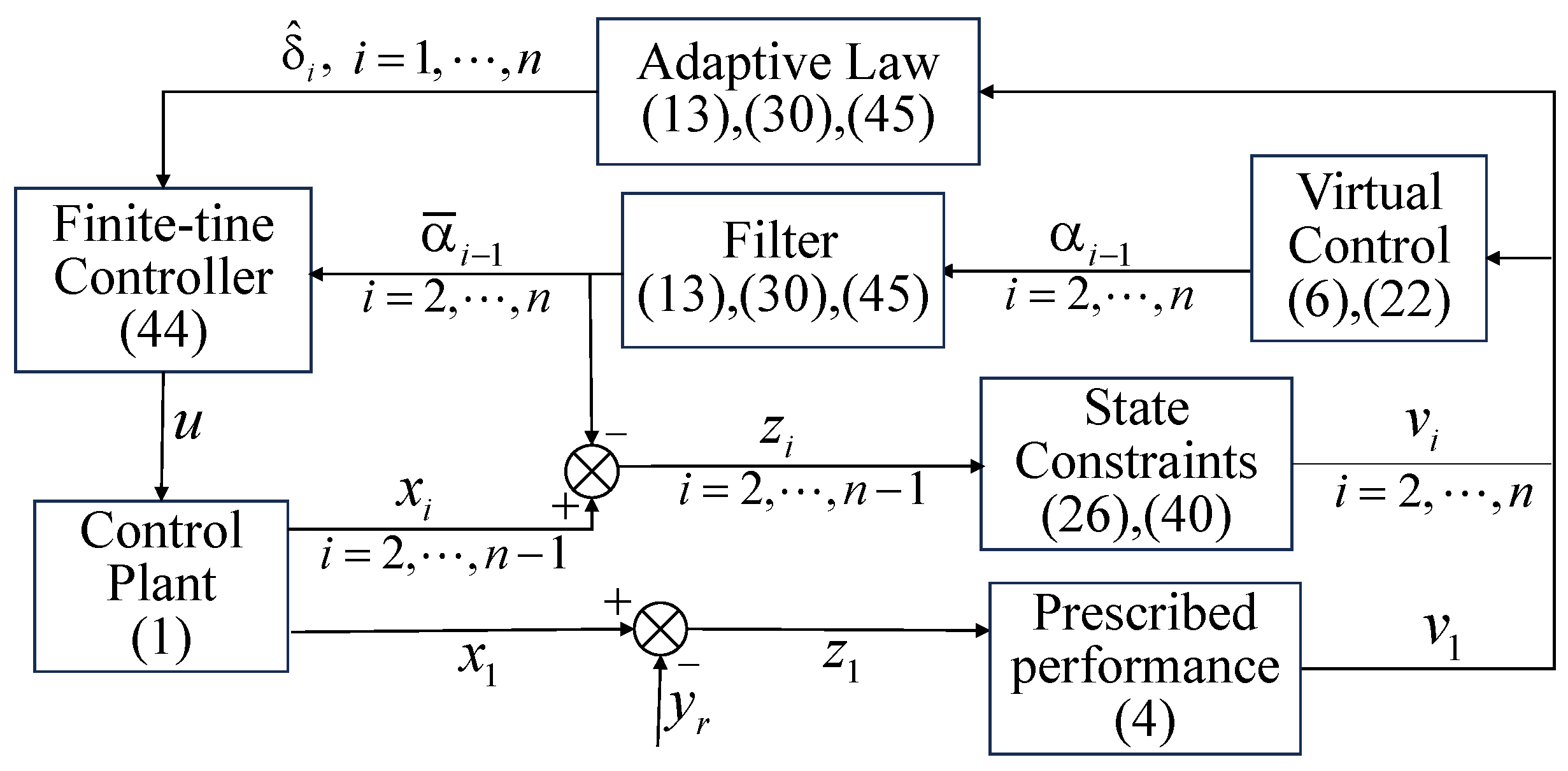
To express the control scheme more clearly, the design procedure of the algorithm is shown in Figure 1.
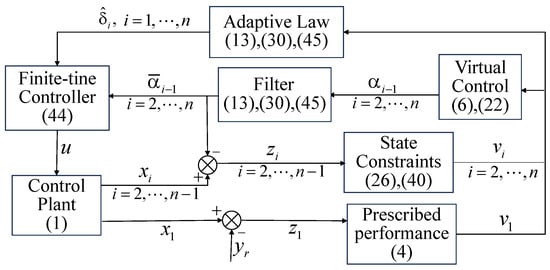
Figure 1.
The block diagram of the control scheme.
4. Numerical Simulations
In this section. the designed controller is compared to two cases to demonstrate its advantages. Case 1, Case 2, and Case 3 represent the control method of this paper proposed, the general BLF control, and the free constraint control, respectively.
Example 1.

Consider the following single-ink rigid robot system:
where is the mass of the rigid link, is the moment of inertia, the angle of joint rotation is , is the load, the gravity coefficient, and the length of the robot link is . The system can be expressed as the following if set , and the dead-zone input are combined.
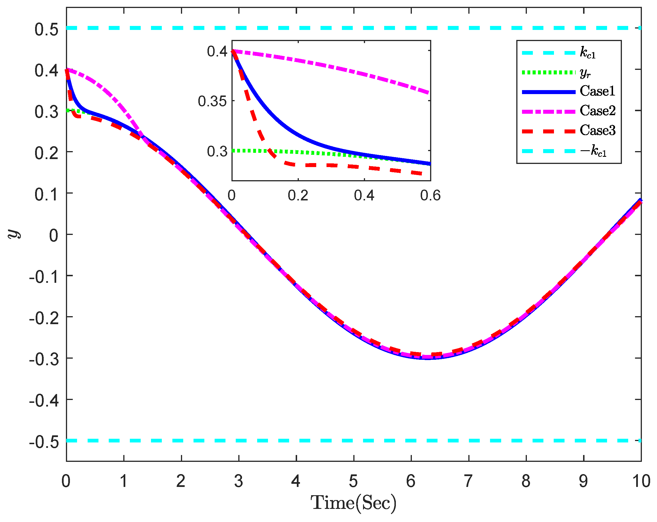
In the simulation, the states are constrained in and . The given tracking signal is . The given performance function is . That is, the steady-state error is allowed not to exceed 0.001. The initial states are set to , , , , and the input parameters of the dead zone are . The parameters are set as , , , . Figure 2, Figure 3, Figure 4, Figure 5, Figure 6 and Figure 7 show the results of the simulation.
Figure 2.
Trajectory of y, , and the constraints , and −.
Figure 3.
Trajectory of and the predefined constraints , and −.
Figure 4.
Trajectory of and the constraints and −.
Figure 5.
Trajectory of and the constraints and −.
Figure 6.
Trajectory of adaptive laws of , and .
Figure 7.
Trajectory of .
From Figure 2, Figure 3, Figure 4 and Figure 5, it is seen that using the control method designed in this paper, y can fast track the reference signal in finite-time, and the state constraints are not violated. Moreover, Figure 6 shows the response of the adaptive law. Figure 7 shows the trajectory of . To further clarify the comparison, some statistics are given in the following.
From Table 1, using the presented control method, the signal is tracked at and the tracking remains stable. The two other methods do not track the reference signal at this time. As can be seen from Table 2, the errors in Case 1 remain within the prescribed range, while the errors in Case 2 and Case 3 exceed the preset range at some moments. Moreover, the mean and RMS of the error are shown in Table 3.
Table 1.
The system output y and the reference signal .
Table 2.
The tracking error and the prescribed performance function .
Table 3.
The mean and RMS of the tracking .
According to Table 4 below, the state remains within the constraint range in Case 1 and Case 2, while the constraint is violated at some moments in Case 3.
Table 4.
The system state .
Example 2.

The second-order strict feedback nonlinear system is as follows.
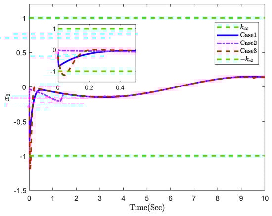
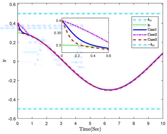
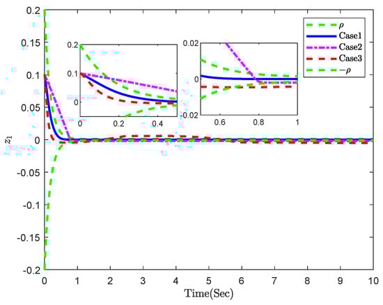
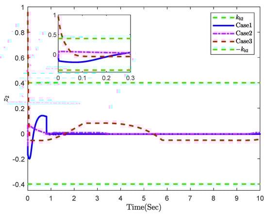
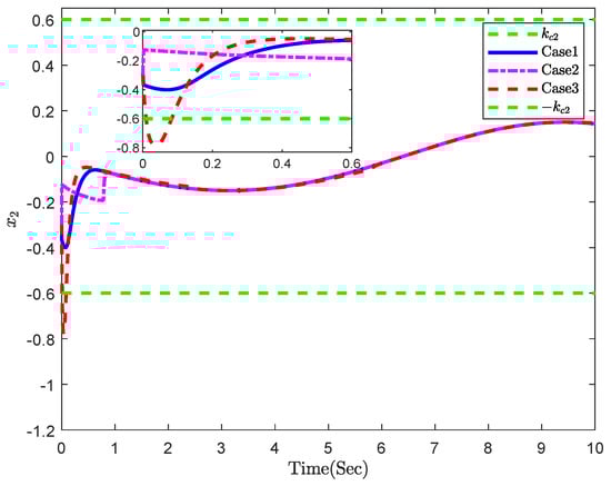
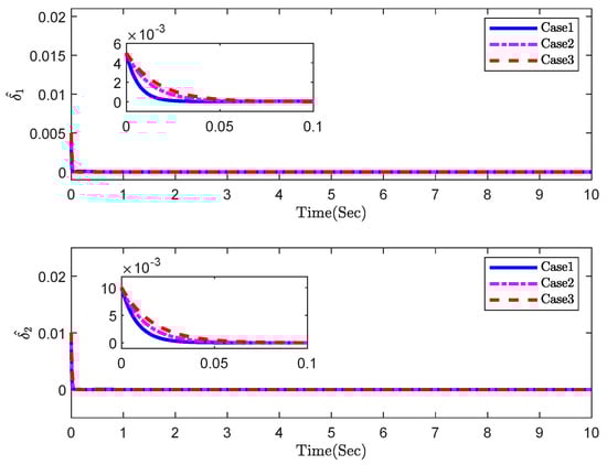
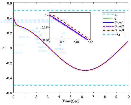
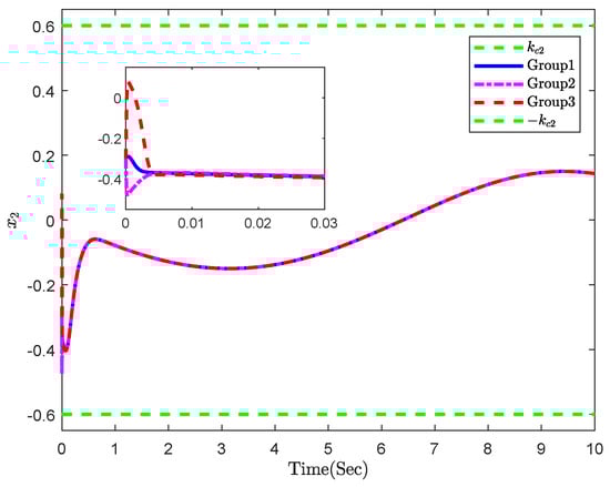
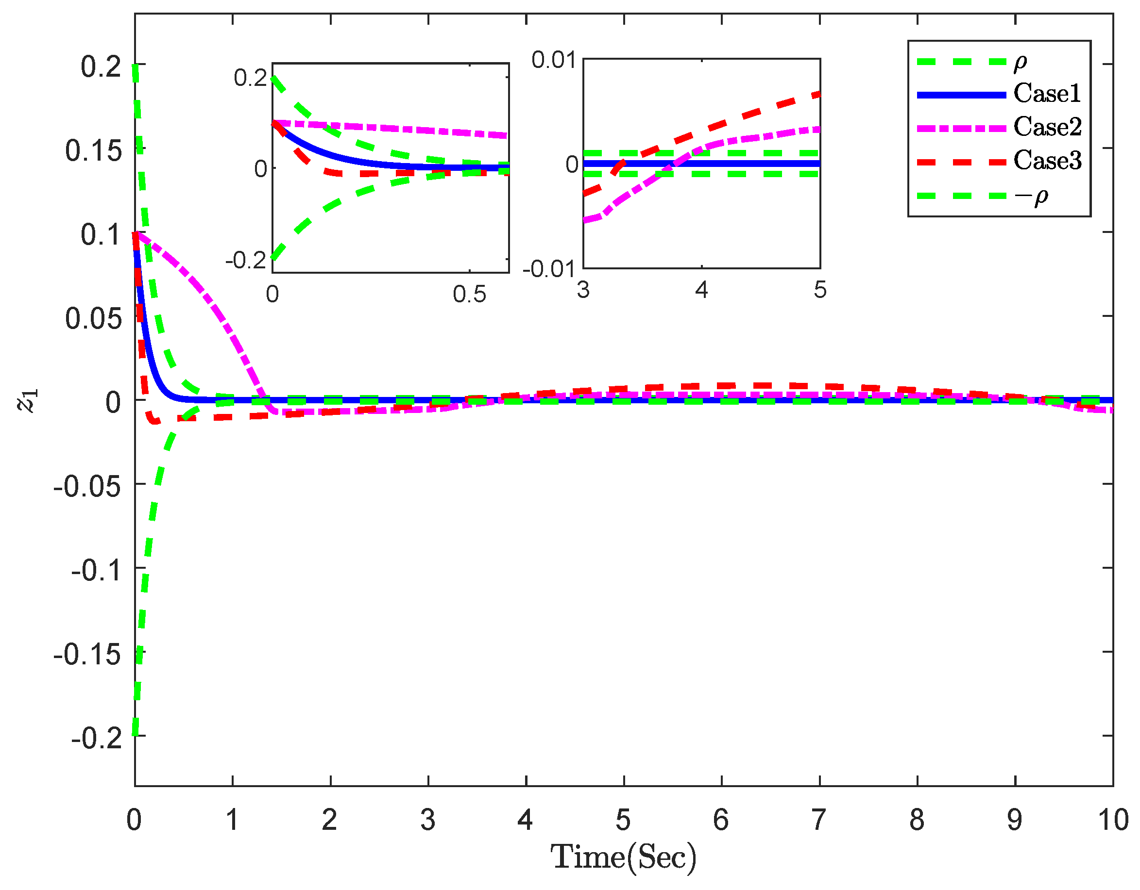
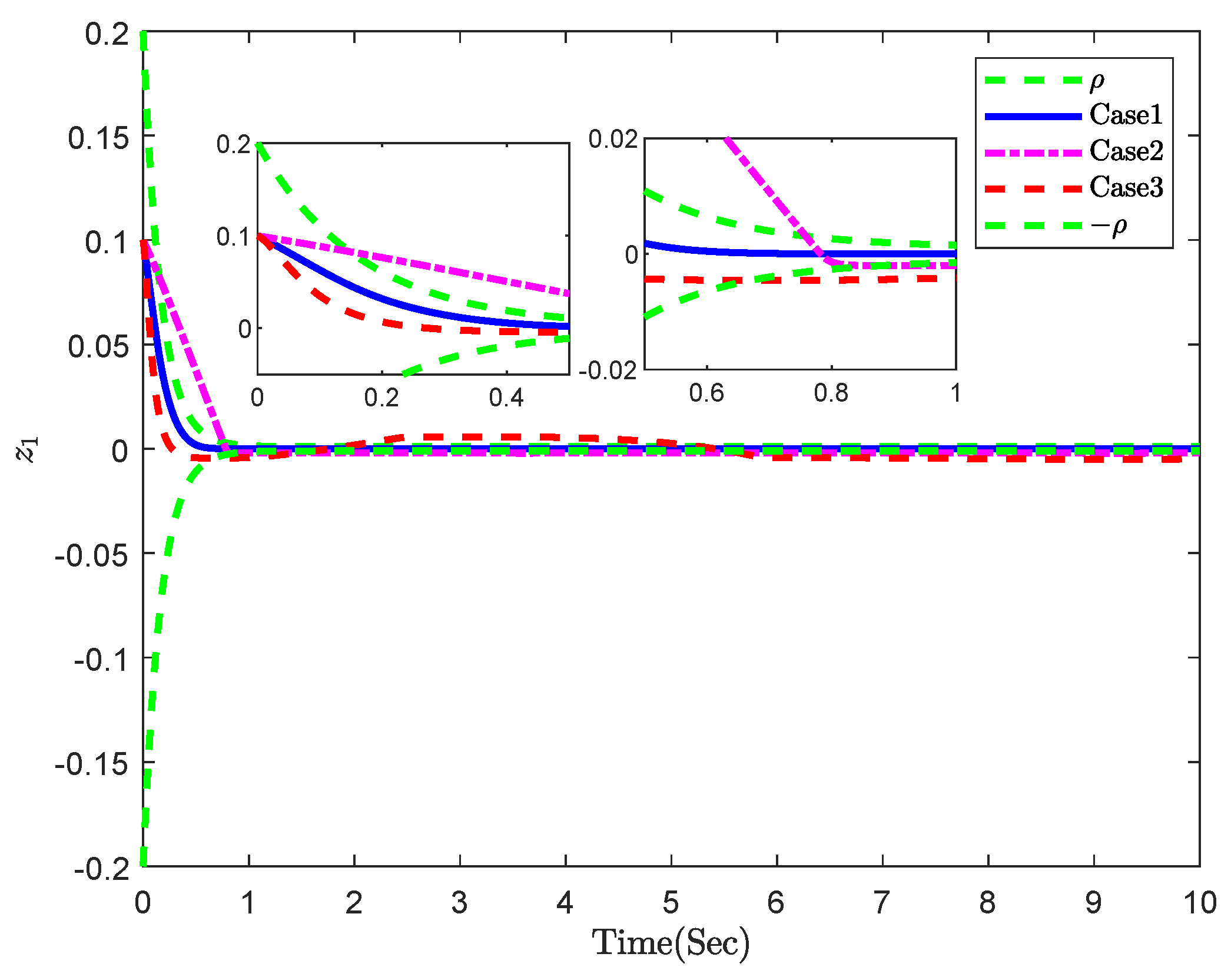
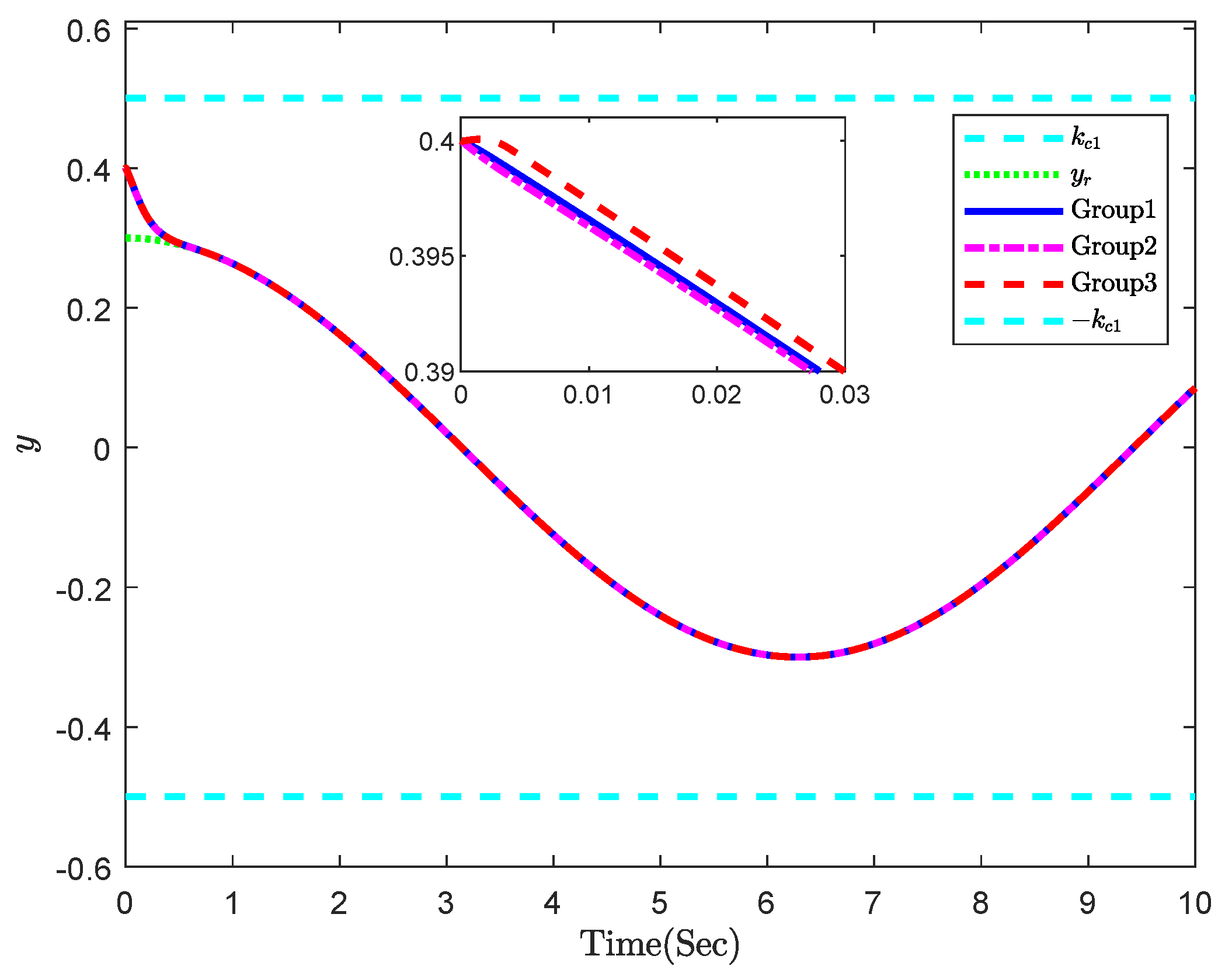
where the states are constrained in and . The initial states are set to , , , . The parameters are set as , , , . The rest is the same as in Example 1. Figure 8, Figure 9, Figure 10, Figure 11, Figure 12 and Figure 13 show the simulation results.
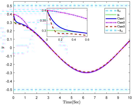
Figure 8.
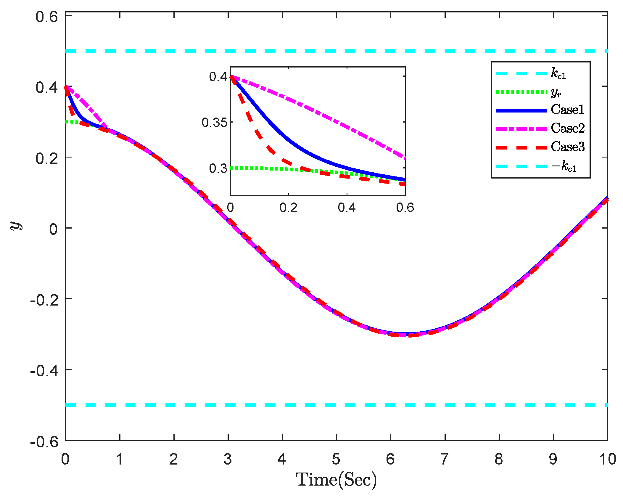
Trajectory of y, , and the constraints and −.
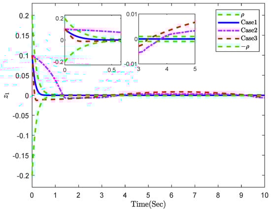
Figure 9.
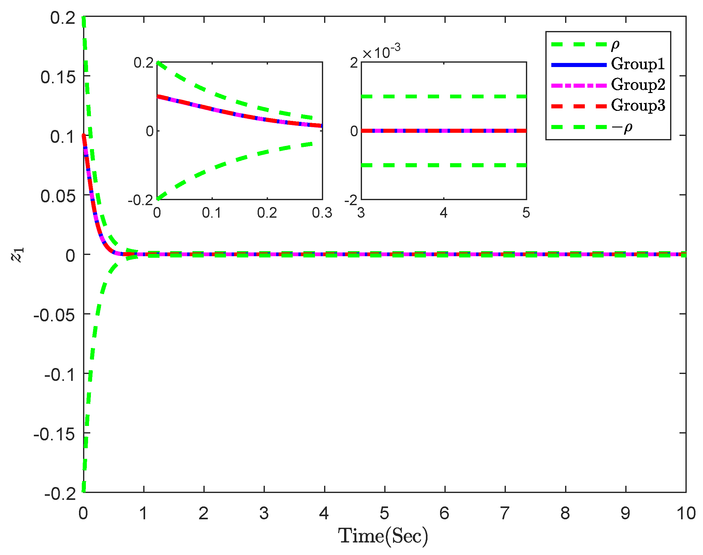
Trajectory of and the predefined constraints and −.
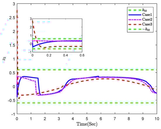
Figure 10.
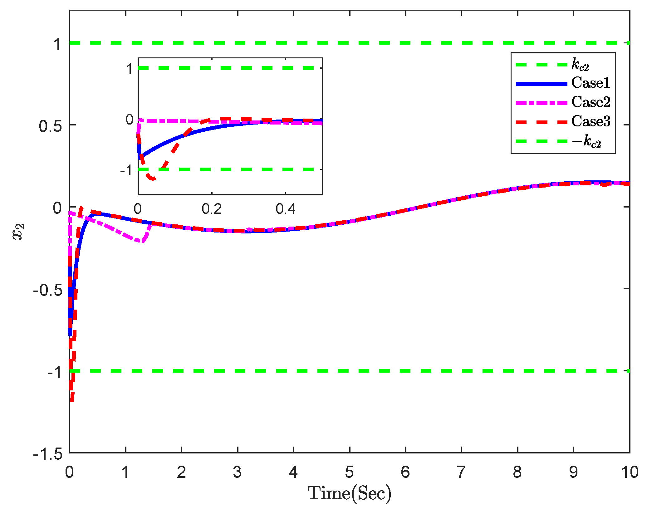
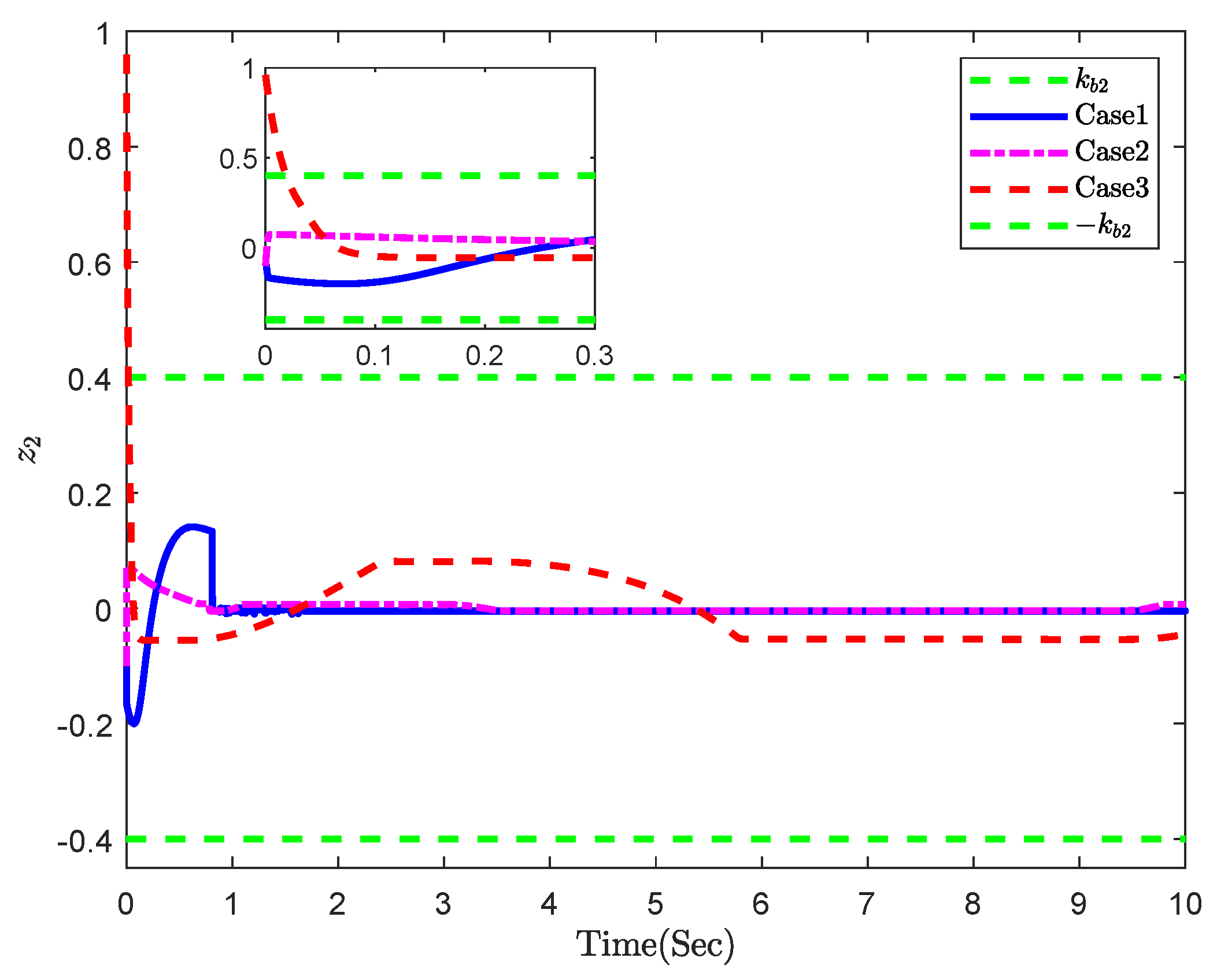
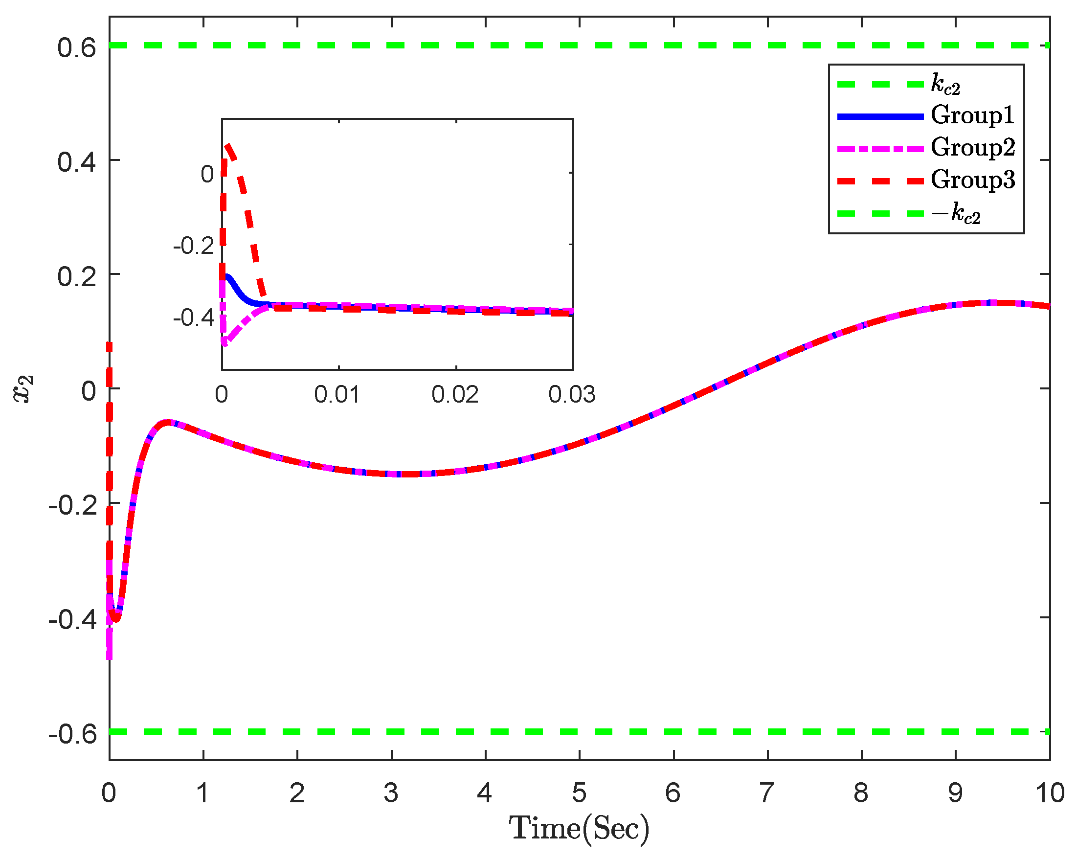
Trajectory of and the constraints and −.
Figure 11.
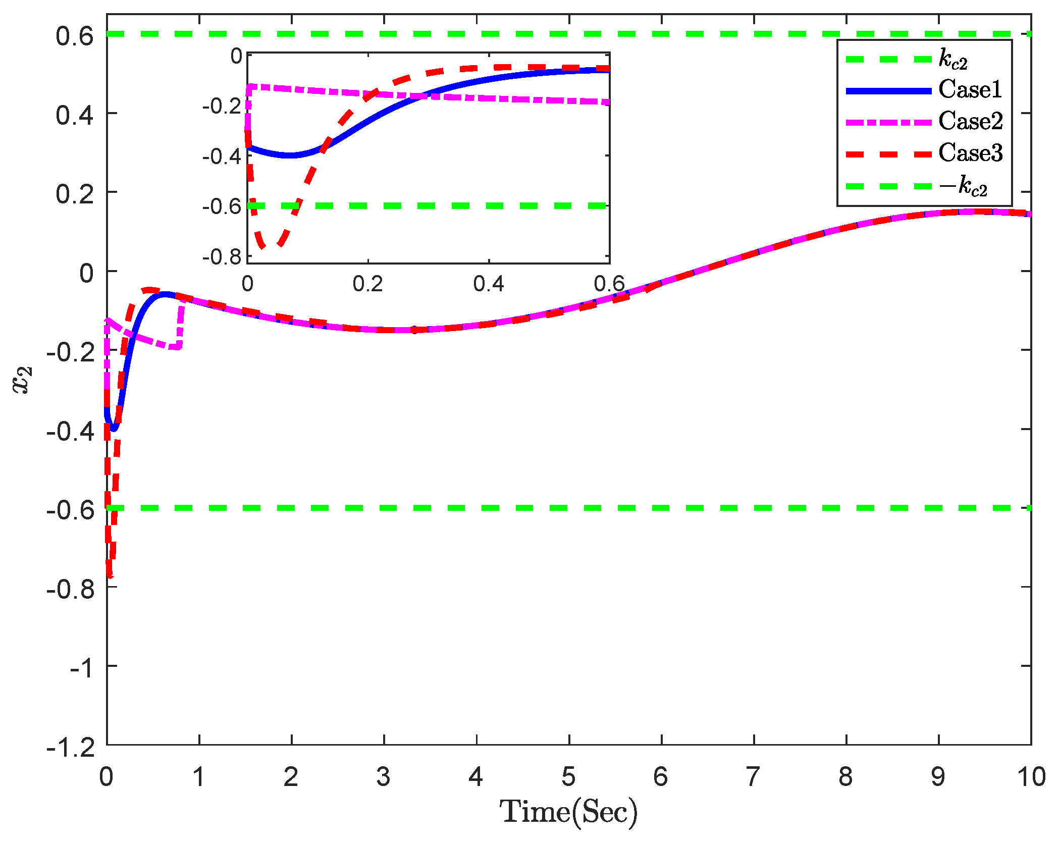
Trajectory of and the constraints and −.
Figure 12.
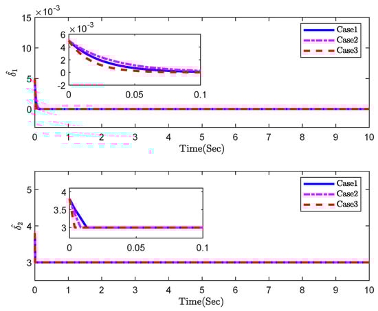
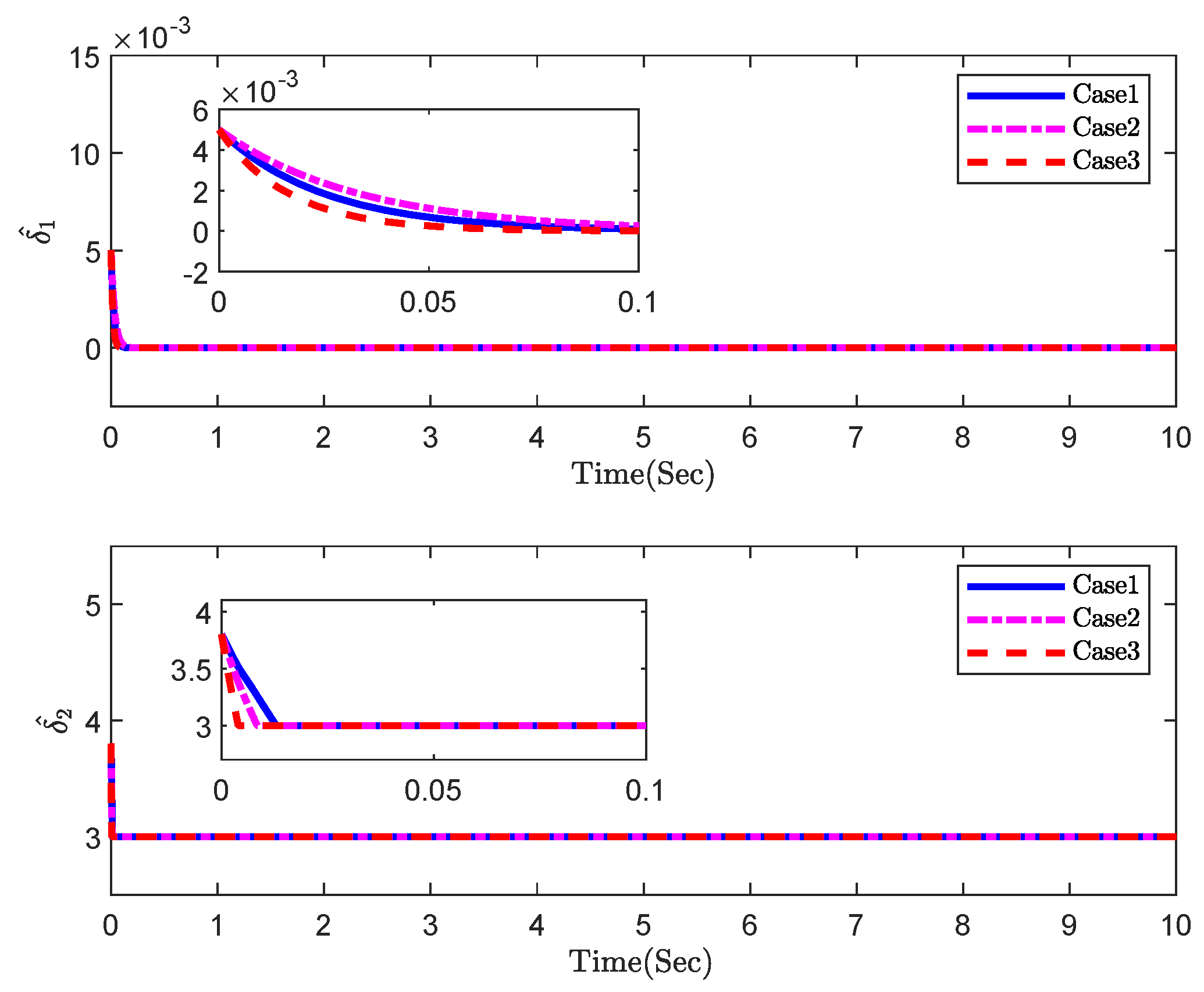
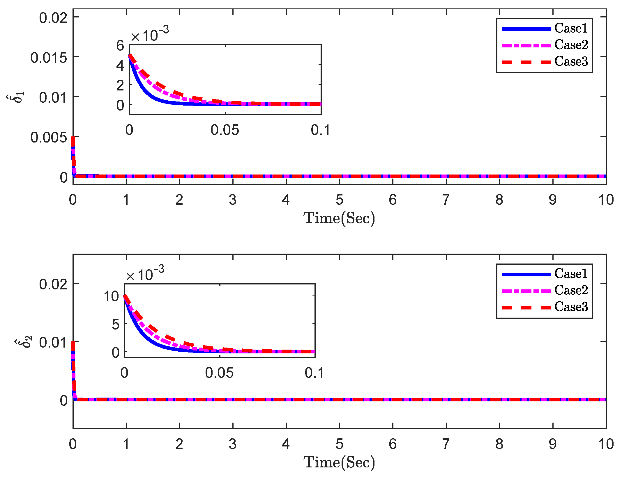
Trajectory of the adaptive laws of and .
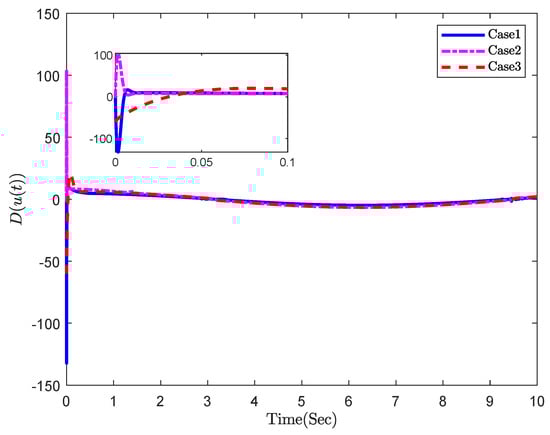
Figure 13.
Trajectory of y, , and the constraints and −.
From Figure 8, Figure 9, Figure 10 and Figure 11, it can be seen that using the control method designed in this paper, y can fast track the reference signal in finite-time, and the state constraints are not violated. Figure 12 shows the response of the adaptive law. Furthermore, some statistics are given in the following.
From Table 5, Table 6 and Table 7. The signal is tracked at t = 1.0217 and the tracking remains stable in Case 1. The other two methods do not track the reference signal at this time. As can be seen from Table 2, the errors in Case 1 remain within the prescribed range, while the errors in Case 2 and Case 3 exceed the preset range at some moments. Furthermore, the mean and RMS of the error are shown in Table 7.
Table 5.
The system output y and the reference signal .
Table 6.
The tracking error and the prescribed performance function .
Table 7.
The mean and RMS of the tracking .
According to Table 8 below, the state remains within the constraint range in Case 1 and Case 2, while the constraint is violated at some moments in Case 3.
Table 8.
The system state .
Moreover, the effect of three different groups of control parameters on the performance of the control system is also investigated. They are, respectively, Group 1, which is , , Group 2, which is , , and Group 3, which is , . Figure 13, Figure 14 and Figure 15 show the results under different parameters.
Figure 14.
Trajectory of and the predefined constraints and −.
Figure 15.
Trajectory of and the constraints and −.
5. Conclusions
The power system satisfies the prescribed performance and full state constraints. This approach ensures that in a finite time, the state variables in the power system reach and remain within the boundary constraints and that the error of the power system from the load frequency, etc., reaches and keeps within a predefined range in a finite time. The future investigation will include considering asymmetric constraints on states and time-varying constraint control. The proposed method will be applied to the study of multi-machine power systems, considering the interconnection between multiple motors; moreover, it will be simulated using a simulation system that more closely resembles the real system.
Author Contributions
X.C.: investigation, methodology, software, writing. S.L. and C.Z.: software, writing. W.W.: investigation, software. All authors have read and agreed to the published version of the manuscript.
Funding
This work was supported by the Major Program of the National Natural Science Foundation of China [U20A20332]; Central Government to Guide local scientific and Technological Development of Hebei Province [216Z1902G]; Innovation Group Program of Hebei province [E2020203174]; Hebei Natural Science Foundation [A2022203024]; Provincial Key Laboratory Performance Subsidy Project [22567612H].
Data Availability Statement
Data are contained within the article.
Acknowledgments
The researchers would like to thank Yanshan University for their support.
Conflicts of Interest
The authors declare no conflicts of interest.
References
- Sariyildiz, E.; Oboe, R.; Ohnishi, K. Disturbance observer-based robust control and its applications: 35th- overview. IEEE Trans. Ind. Electron. 2020, 67, 2024–2053. [Google Scholar] [CrossRef]
- Ding, S.; Park, J.H.; Chen, C.-C. Second-order sliding mode controller design with output constraint. Automatica 2020, 112, 108704. [Google Scholar] [CrossRef]
- Labbadi, M.; Cherkaoui, M. Robust adaptive nonsingular fast terminal sliding-mode tracking control for an uncertain quadrotor UAV subjected to disturbances. ISA Trans. 2020, 99, 290–304. [Google Scholar] [CrossRef] [PubMed]
- Han, Y.; Zhang, H.; Shi, Z.; Liang, S. An adaptive fuzzy control model for multi-joint manipulators. Comput. Syst. Sci. Eng. 2021, 40, 1043–1057. [Google Scholar] [CrossRef]
- Tong, S.; Min, X.; Li, Y. Observer-based adaptive fuzzy tracking control for strict-feedback nonlinear systems with unknown control gain functions. IEEE Trans. Cybern. 2020, 50, 3903–3913. [Google Scholar] [CrossRef] [PubMed]
- Liu, C.; Wen, G.; Zhao, Z.; Sedaghati, R. Neural-network-based sliding-mode control of an uncertain robot using dynamic model approximated switching gain. IEEE Trans. Cybern. 2021, 51, 2339–2346. [Google Scholar] [CrossRef] [PubMed]
- Cao, Z.; Niu, Y.; Zou, Y. Adaptive neural sliding mode control for singular semi-markovian jump systems against actuator attacks. IEEE Trans. Syst. Man Cybern. Syst. 2021, 51, 1523–1533. [Google Scholar] [CrossRef]
- Liu, L.; Liu, Y.-J.; Chen, A.Q.; Tong, S.C.; Chen, C.L.P. Integral barrier Lyapunov function-based adaptive control for switched nonlinear systems. Sci. China Inf. Sci. 2020, 63, 132203. [Google Scholar] [CrossRef]
- Liang, H.; Liu, G.; Zhang, H.; Huang, T. Neural-network-based event-triggered adaptive control of nonaffine nonlinear multiagent systems with dynamic uncertainties. IEEE Trans. Neural Netw. Learn. Syst. 2021, 32, 2239–2250. [Google Scholar] [CrossRef]
- Wang, M.; Wang, Z.; Dong, H.; Han, Q.-L. A novel framework for backstepping-based control of discrete-time strict-feedback nonlinear systems with multiplicative noises. IEEE Trans. Autom. Control 2021, 66, 1484–1496. [Google Scholar] [CrossRef]
- Luo, S.; Hu, X.; Zhao, L.; Li, S. Event-triggered neural adaptive backstepping control of the K chaotic PMSGs coupled system. Int. J. Elect. Power Energy Syst. 2022, 135, 107475. [Google Scholar] [CrossRef]
- Rodríguez-Abreo, O.; Ornelas-Rodríguez, F.-J.; Ramírez-Pedraza, A.; HurtadoRamos, J.B.; González-Barbosa, J.-J. Backstepping control for a UAV-manipulator tuned by Cuckoo Search algorithm. Rob. Auton. Syst. 2022, 147, 103910. [Google Scholar] [CrossRef]
- Guo, Q.; Li, X.; Jiang, D. Full-state error constraints based dynamic surface control of electro-hydraulic system. IEEE Access 2018, 6, 53092–53101. [Google Scholar] [CrossRef]
- Liu, Y.-J.; Tong, S. Barrier Lyapunov functions for Nussbaum gain adaptive control of full state constrained nonlinear systems. Automatica 2017, 76, 143–152. [Google Scholar] [CrossRef]
- He, W.; Yin, Z.; Sun, C. Adaptive neural network control of a marine vessel with constraints using the asymmetric barrier Lyapunov Function. IEEE Trans. Cybern. 2017, 47, 1641–1651. [Google Scholar] [CrossRef] [PubMed]
- Liu, Y.-J.; Lu, S.; Tong, S.; Chen, X.; Chen, C.L.P.; Li, D.-J. Adaptive control-based Barrier Lyapunov Functions for a class of stochastic nonlinear systems with full state constraints. Automatica 2018, 87, 83–93. [Google Scholar] [CrossRef]
- Gao, T.; Liu, Y.-J.; Liu, L.; Li, D. Adaptive neural Network-Based control for a class of Nonlinear Pure-Feedback systems with time-varying full state constraints. IEEE/CAA J. Autom. Sin. 2018, 5, 923–933. [Google Scholar] [CrossRef]
- Ma, H.; Li, H.; Liang, H.; Dong, G. Adaptive fuzzy event-triggered control for stochastic nonlinear systems with full state constraints and actuator faults. IEEE Trans. Fuzzy Syst. 2019, 27, 2242–2254. [Google Scholar] [CrossRef]
- Cao, L.; Zhou, Q.; Dong, G.; Li, H. Observer-Based adaptive event-triggered control for Nonstrict-Feedback nonlinear systems with output constraint and actuator failures. IEEE Trans. Syst. Man Cybern. Syst. 2021, 51, 1380–1391. [Google Scholar] [CrossRef]
- Sun, W.; Su, S.-F.; Wu, Y.; Xia, J. Novel adaptive fuzzy control for output constrained stochastic nonstrict feedback nonlinear systems. IEEE Trans. Fuzzy Syst. 2021, 29, 1188–1197. [Google Scholar] [CrossRef]
- Sun, W.; Su, S.-F.; Dong, G.; Bai, W. Reduced adaptive fuzzy tracking control for high-order stochastic nonstrict feedback nonlinear system with full-state constraints. IEEE Trans. Syst. Man Cybern. Syst. 2021, 51, 1496–1506. [Google Scholar] [CrossRef]
- Wu, Y.; Xie, X.-J. Robust adaptive control for state-constrained nonlinear systems with input saturation and unknown control direction. IEEE Trans. Syst. Man Cybern. Syst. 2021, 51, 1192–1202. [Google Scholar] [CrossRef]
- Tee, K.P.; Ge, S.S. Control of nonlinear systems with partial state constraints using a barrier Lyapunov function. Int. J. Control 2011, 84, 2008–2023. [Google Scholar] [CrossRef]
- Zhao, Z.; Ahn, C.K. Boundary output constrained control for a flexible beam system with prescribed performance. IEEE Trans. Syst. Man Cybern. Syst. 2021, 51, 4650–4658. [Google Scholar] [CrossRef]
- Liu, Y.-J.; Zeng, Q.; Tong, S.; Chen, C.L.P.; Liu, L. Actuator failure compensation-based adaptive control of active suspension systems with prescribed performance. IEEE Trans. Ind. Electron. 2020, 67, 7044–7053. [Google Scholar] [CrossRef]
- Qiu, J.; Sun, K.; Wang, T.; Gao, H. Observer-Based fuzzy adaptive event-triggered control for pure-feedback nonlinear systems with prescribed performance. IEEE Trans. Fuzzy Syst. 2019, 27, 2152–2162. [Google Scholar] [CrossRef]
- Sun, K.; Qiu, J.; Karimi, H.R.; Gao, H. A novel finite-time control for nonstrict feedback saturated nonlinear systems with tracking error constraint. IEEE Trans. Syst. Man Cybern. Syst. 2021, 51, 3968–3979. [Google Scholar] [CrossRef]
- Si, W.; Qi, L.; Hou, N.; Dong, X. Finite-time adaptive neural control for uncertain nonlinear time-delay systems with actuator delay and full-state constraints. Int. J. Syst. Sci. 2019, 50, 726–738. [Google Scholar] [CrossRef]
- Li, Y.; Yang, T.; Tong, S. Adaptive neural networks finite-time optimal control for a class of nonlinear systems. IEEE Trans. Neural Netw. Learn. Syst. 2020, 31, 4451–4460. [Google Scholar] [CrossRef]
- Ma, L.; Zong, G.; Zhao, X.; Huo, X. Observed-based adaptive finite-time tracking control for a class of nonstrict-feedback nonlinear systems with input saturation. J. Frankl. Inst. 2020, 357, 11518–11544. [Google Scholar] [CrossRef]
- Wang, H.; Liu, P.X.; Zhao, X.; Liu, X. Adaptive fuzzy finite-time control of nonlinear systems with actuator faults. IEEE Trans. Cybern. 2020, 50, 1786–1797. [Google Scholar] [CrossRef] [PubMed]
- Na, J.; Huang, Y.; Wu, X.; Su, S.-F.; Li, G. Adaptive finite-time fuzzy control of nonlinear active suspension system with input delay. IEEE Trans. Cybern. 2020, 50, 2639–2650. [Google Scholar] [CrossRef] [PubMed]
- Wang, N.; Karimi, H.R.; Li, H.; Su, S.-F. Accurate Trajectory Tracking of Disturbed Surface Vehicles: A Finite-Time Control Approach. IEEE/ASME Trans. Mechatronics 2019, 24, 1064–1074. [Google Scholar] [CrossRef]
- Pan, H.; Sun, W. Nonlinear output feedback finite-time control for vehicle active suspension systems. IEEE Trans. Ind. Informat. 2019, 15, 2073–2082. [Google Scholar] [CrossRef]
- Wang, F.; Chen, B.; Liu, X.; Lin, C. Finite-Time adaptive fuzzy tracking control design for nonlinear systems. IEEE Trans. Fuzzy Syst. 2018, 26, 1207–1216. [Google Scholar] [CrossRef]
- Wu, Q.; Dong, S.; Zhang, W.-A.; Yu, L. Online modeling of the CNC engraving system with Dead-Zone input nonlinearity. IEEE Trans. Ind. Electron. 2022, 69, 774–782. [Google Scholar] [CrossRef]
- Ma, L.; Huo, X.; Zhao, X.D.; Zong, G.D. Observer-based adaptive neural tracking control for output-constrained switched MIMO nonstrict-feedback nonlinear systems with unknown dead zone. Nonlinear Dyn. 2020, 99, 1019–1036. [Google Scholar] [CrossRef]
- Wang, S.; Yu, H.; Yu, J.; Na, J.; Ren, X. Neural-Network-Based adaptive funnel control for servo mechanisms with unknown Dead-Zone. IEEE Trans. Cybern. 2020, 50, 1383–1394. [Google Scholar] [CrossRef] [PubMed]
- Li, Z.; Li, T.; Feng, G.; Zhao, R.; Shan, Q. Neural Network-Based adaptive control for pure-feedback stochastic nonlinear systems with Time-Varying delays and Dead-Zone input. IEEE Trans. Syst. Man Cybern. Syst. 2020, 50, 5317–5329. [Google Scholar] [CrossRef]
- Yang, T.; Sun, N.; Chen, H.; Fang, Y. Neural Network-Based adaptive antiswing control of an underactuated Ship-Mounted crane with roll motions and input dead zones. IEEE Trans. Neural Netw. Learn. Syst. 2020, 31, 901–914. [Google Scholar] [CrossRef]
- Zhu, Z.; Xia, Y.; Fu, M. Attitude stabilization of rigid spacecraft with finite time convergence. Int. J. Robust Nonlinear Control 2011, 21, 686–702. [Google Scholar] [CrossRef]
- Wang, F.; Chen, B.; Lin, C.; Zhang, J.; Meng, X. Adaptive neural network finite-time output feedback control of quantized nonlinear systems. IEEE Trans. Cybern. 2018, 48, 1839–1848. [Google Scholar] [CrossRef] [PubMed]
- Qian, C.; Lin, W. Non-Lipschitz continuous stabilizers for nonlinear systems with uncontrollable unstable linearization. Syst. Control Lett. 2001, 42, 185–200. [Google Scholar] [CrossRef]
- Yu, J.; Shi, P.; Zhao, L. Finite-time command filtered backstepping control for a class of nonlinear systems. Automatica 2018, 92, 173–180. [Google Scholar] [CrossRef]


Disclaimer/Publisher’s Note: The statements, opinions and data contained in all publications are solely those of the individual author(s) and contributor(s) and not of MDPI and/or the editor(s). MDPI and/or the editor(s) disclaim responsibility for any injury to people or property resulting from any ideas, methods, instructions or products referred to in the content. |
© 2024 by the authors. Licensee MDPI, Basel, Switzerland. This article is an open access article distributed under the terms and conditions of the Creative Commons Attribution (CC BY) license (https://creativecommons.org/licenses/by/4.0/).