Impact of Train Formation on the Dynamic Responses and Operational Safety of High-Speed Trains under Non-Uniform Seismic Ground Motion

Abstract

The study of dynamic responses and operational safety of high-speed trains under seismic excitation has increasingly relied on numerical simulation as the most effective and convenient research approach. The majority of studies only focus on single-car formation, and fewer utilize train models with actual standard formation, inevitably resulting in differences in dynamic characteristics of train models and simulation results. Furthermore, trains also have different standard formations in different countries and operating scenarios. Therefore, the influences of train formation on the dynamic responses and operational safety of trains under seismic action are investigated. Hence, a detailed train/vehicle–track coupled dynamics model was established to simulate trains under non-uniform seismic ground motion. Moreover, due to wheel–rail contact simulation being the key factor constraining simulation efficiency, based on the influence pattern of train formation, whether fewer train formations can achieve the same simulation accuracy as the 8-car standard formation is also explored in this paper considering seismic wave propagation effect. Results indicate that variation in train formation can influence the dynamic responses of a coupled system significantly from both the perspective of wheel–rail interaction and vehicle kinematic responses. Moreover, the 5-car formation model can better meet the accuracy requirement and significantly improve computational efficiency compared to 8-car formation model.

1. Introduction

The public steadily comes to rely on railway transportation as a necessary means of transportation due to its safety, speed, punctuality, environmental friendliness, and low energy consumption, all of which are becoming more and more desirable as travel demands rise. High-speed railway networks are being rapidly expanded in many countries. China has gone through a phase of fast railway construction development in recent years. As of the end of 2022, China’s railway has achieved a total length of 155,000 km, with 42,000 km of high-speed railway, both ranking first in the world. However, due to China’s large land area, intricate geological structure, and frequent widespread earthquakes, it is inevitable that railway lines would be constructed in seismically active areas, endangering both the security of people and property as well as train operations safety. Specifically, earthquakes have caused several train derailments in Japan. Notably, on 16 June 2004, a Shinkansen train named “Tsubame No. 325” that was traveling between Urasa and Nagaoka was derailed by a 6.8-magnitude earthquake that struck Niigata [1]. A Shinkansen 800 series train derailed on 14 April 2016, as a result of the Kumamoto earthquake. Moreover, on 16 March 2022, a 7.4-magnitude earthquake close to Fukushima Prefecture’s coast resulted in the Tohoku Shinkansen “Hayabusa No. 223” derailment and significant tilting. Consequently, research into the dynamic responses, mechanisms, and seismic overturning resistance of railway cars under seismic action has gained attention due to the crucial importance of railway transport and previous incidents. The research findings can offer crucial protections for the secure functioning of railway vehicles.

Many scholars have been conducting extensive studies in the field of railway earthquake resistance in the last few years. Japanese researchers Miyamoto et al. [2,3,4] conducted a series of experimental and theoretical studies on the thresholds of train operational safety and derailment mechanisms under seismic action. The results showed that vertical seismic motions significantly impact wheel lift and wheel load reduction, but horizontal seismic excitation plays a dominant role in vehicle derailment. Kazuhiko Nishimura et al. [5] developed a vehicle–track coupled model containing 14 degrees of freedom (DOFs), whose accuracy was validated through full-scale static and dynamic tests, to explore the derailment mechanism of high-speed trains during intense seismic motions. Their research emphasizes that the vehicle body’s roll motion and wheelsets’ lateral motion are the main indicators for assessing train derailment, with the degree of lateral sliding of the wheelset being proportional to the operating speed. Ju et al. [6] established a detailed finite element model with a train–track–embankment coupled system to investigate the influences of operating speed, track irregularities, field types, and seismic motion characteristics on derailment coefficient. The numerical results demonstrated that when track irregularities are present, the derailment coefficient of each wheelset is positively correlated with the operating speed. Additionally, seismic motion records from soft soil areas are rich in low-frequency components, which are more likely to resonate with the train, leading to larger vibrations and increasing derailment risk. Yang et al. [7] investigated the dynamic behaviors of the train-cable-stayed-bridge coupled system in seismic scenarios by establishing a detailed full-scale three-dimensional (3D) finite element (FE) model. Through a series of parametric analyses, they found both the train dynamic responses and safety indicators are positively correlated with the train operating speed and seismic intensity. Based on this, authors introduced a threshold curve governed by peak ground acceleration (PGA) and operating speed. Cheng et al. [8] employed a nonlinear creep model to study the dynamic behaviors of tilting railway vehicles operating on curved tracks and subjected to seismic and wind loads. The results indicate that tilting railway vehicles possess a higher risk of derailment compared to non-tilting railway vehicles, regardless of track irregularities and environmental loads. Zeng et al. [9] developed the Train–Bridge Interaction Analysis Program (SVBI) to assess the dynamic safety of high-speed trains operating on elevated bridges during intense seismic motions. Through comparative analysis with ground-level conditions, they found that seismic-induced movements of bridges can intensify the dynamic reactions of trains, consequently elevating the risk of derailment. Tanabe et al. [10] employed multibody dynamics and finite element methods to simulate and analyze the dynamic responses of trains and railway structures, aiming to address the dynamic interactions between high-speed trains and track structures during earthquakes, including derailment and post-derailment behaviors. Chen et al. [11] established a train–track–bridge coupled model with 16 carriages to comparatively analyze the influences of near-field and far-field seismic motions on a coupled system. The study showed that near-field seismic motions significantly enhanced the mid-span and pier-top movements of the bridge and wheel–rail interaction level compared to far-field seismic motions. Zhou et al. [12,13,14] proposed an effective simplified model to improve the computational efficiency of the train–track–bridge coupled system during uniform seismic excitations. By constructing virtual elements to virtually connect both ends of the track and bridge, trains are enabled to operate on a hypothetical circular track model, significantly reducing the calculation scale of track and bridge. Subsequently, this simplified model was then used for analyzing the influences of near-fault pulse-type ground motions on the operational security of high-speed trains. A 1:10 scale test using an array of four sub-shaking tables is performed by Yu et al. [15] to study the dynamic behaviors of trains during seismic action and explored impacts and damping effects of train operations on track and bridge structures. The experimental results indicate that train operations have a significant impact on track structures but a minimal effect on bridge structures. Jiang et al. [16] established a FE model of the vehicle–track-continuum simply supported beam bridge system and studied impacts of track irregularities on the train’s dynamic behaviors and analyzed its probabilistic statistical characteristics. Based on their findings, a standard value for the track irregularity influence coefficient based on a probability assurance rate was proposed. Zhao et al. [17] introduced a novel predictive method (NPEM) to investigate the operational safety of high-speed trains on simply supported bridges during earthquakes, considering seismic wave propagation effects. It reveals significant influences of seismic parameter uncertainties on operational safety and provides new insights and methodologies for understanding and improving the design and maintenance of railway bridges. Fang et al. [18] mainly explored the impacts of site conditions on the train–track–bridge coupled systems during seismic action. Through shake table tests and dynamic model analysis, they also investigated the impacts of lateral seismic motion on the safe operating speed thresholds. The findings indicated that site conditions do play a vital role in operating safety and that both system responses and safety indicators increase with PGA and operating speed.

The research presented above explores the dynamic response patterns of trains during seismic ground motion, offering crucial insights into improving operational safety in the event of unexpected earthquakes. However, it is worth mentioning that most existing research primarily concentrates on single-car formation, and fewer studies make use of trains with actual standard formation, such as 8-car formation or 16-car formation. Nevertheless, varying train configurations will unavoidably result in disparities in simulation results for the identical analysis matter. Moreover, trains can exhibit distinct standard configurations in different countries and operational circumstances. Hence, it is imperative to examine the interaction effects between neighboring vehicles and influences of train configuration on the dynamic behaviors and safety analysis of trains subjected to seismic activities. In addition, the majority of studies only consider uniform seismic input; however, vibrations along railway lines during an earthquake occurrence typically are not uniformly distributed across different sites. Therefore, the influence of seismic wave propagation is also considered simultaneously in this paper.

Considering the negative correlation between the count of wheel–rail contact points and simulation speed, for this reason, if influence patterns of train formation are determined, is it feasible for fewer train formations to attain the same degree of simulation accuracy as the actual formation? It is worth further investigation. In the above-presented studies, when trains are formed with only one vehicle, the effects of inter-carriage coupling on the overall dynamic behavior of the trains are ignored, which can result in underestimation of wheel–rail interactions as well as significant deviations in the results. Alternatively, some scholars have utilized train models with real standard formations, such as the 8-car or 16-car formation model, in order to improve computational accuracy and reliability. However, this modeling method leads to reduced computing performance and increased resource consumption. Moreover, the inherent unpredictability of earthquake occurrences makes it impossible to conduct on-site tests. Moreover, laboratory testing encounters numerous constraints and restrictions. Usually, these tests require trains to be stationary relative to track structure, which creates a testing environment that significantly deviates from real operational conditions and results in significant expenses. Therefore, numerical simulation remains the primary research methodology. Based on this, it is imperative to explore the optimal quantity of railway vehicles for numerical simulations, taking into account non-uniform seismic ground motion, aiming to achieve a compromise between simulation accuracy and simulation efficiency. In nations such as China, a standard electric multiple unit (EMU) high-speed train usually comprises eight carriages; hence, the numerical results of the 8-car formation model are treated as benchmarks in this paper.

2. Methodology

A comprehensive vehicle/train–track coupled model is essential for analyzing dynamic responses and operational safety of trains under seismic excitations. In this section, according to theories of vehicle–track coupled dynamics [19], a four-axle vehicle multibody model and a twin-block ballastless track model are respectively developed. Additionally, the functions of inter-carriage connection devices are fully considered, allowing for the assembly of individual vehicle models into a train model to enable comprehensive simulations.

2.1. Vehicle Model

A vehicle model is composed of the following seven components: one vehicle body, two bogie frames, and four wheelsets, and all are represented as rigid bodies. In addition, two sets of suspension systems are also established using springs and dampers to buffer relative motion between adjacent components and mitigate dynamic responses. In this study, anti-roll springs, lateral stop devices, and traction rods are considered thoroughly, which are frequently overlooked in previous research. Nevertheless, the influences of them on the high-speed trains’ dynamic responses under extreme operating conditions cannot be disregarded.

Each rigid body has a total of 6 DOFs, including translational movements (longitudinal, lateral, and heave) as well as rotational movements (roll, pitch, and yaw). Therefore, a single vehicle possesses 42 DOFs. Detailed DOFs of one single vehicle model are summarized in Table 1. Views of one single vehicle model from three directions are exhibited in Figure 1, Figure 2 and Figure 3. Detailed descriptions and specific values of each physical quantity are tabulated in Table A1.

Table 1. DOFs of single vehicle model.

DOFs	Longitude	Lateral	Heave	Roll	Pitch	Yaw
Vehicle body	Xc	Yc	Zc	Φc	βc	Ψc
Front bogie frame	Xt1	Yt1	Zt1	Φt1	βt1	Ψt1
Rear bogie frame	Xt2	Yt2	Zt2	Φt2	βt2	Ψt2
1st wheelset	Xw1	Yw1	Zw1	Φw1	βw1	Ψw1
2nd wheelset	Xw2	Yw2	Zw2	Φw2	βw2	Ψw2
3rd wheelset	Xw3	Yw3	Zw3	Φw3	βw3	Ψw3
4th wheelset	Xw4	Yw4	Zw4	Φw4	βw4	Ψw4

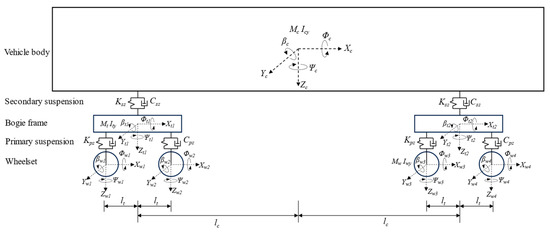
Figure 1. Side view of the vehicle subsystem.

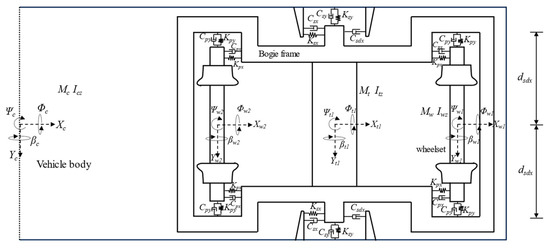
Figure 2. Top view of the vehicle subsystem.

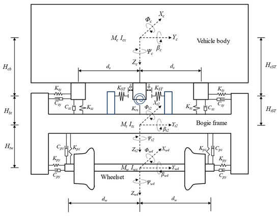
Figure 3. End view of the vehicle subsystem.

2.2. Inter-Carriage Connection Devices

In existing research regarding multi-car train formations, some studies assume that the interaction between adjacent vehicles is minor, resulting in the omission of modeling the inter-carriage connection devices [20]. Conversely, other studies use spring elements to simulate the elastic connections of adjacent vehicle bodies [21]. However, due to the rapid development of high-speed trains and growing operating speed, especially under extreme operating conditions (e.g., earthquake, crosswind), the connection devices between vehicle bodies are crucial in determining the mechanical behaviors of the entire train subsystem compared to traditional trains. Therefore, neglecting inter-carriage connection devices or representing them with spring elements will cause significant simulation errors. Therefore, this study primarily considers three types of inter-carriage connection devices, i.e., coupler draft gear, longitudinal vibration absorption device, and tightly sealed windshield. Although the method of simulating inter-carriage connection devices was proposed by [22], it has not yet been widely employed in the study of railway train seismic resistance. This section outlines the mechanical models for these three types of inter-carriage connection devices.

2.2.1. Coupler Draft Gear

In this study, the coupler draft gear is conceptualized as a spatial two-force member, only capable of axial elongation and compression, and hinged at the centers of the bases of adjacent vehicle body ends. For simplification, the mass is neglected. The coupler draft gear’s nonlinear stiffness characteristics, including the gap, are simulated using a bilinear model, as shown in Figure 4. The force $F_{cg}$ generated by coupler draft gear can be represented by Equation (1).

$$F_{cg}=\{\begin{array}{ll}0& |\Delta x|<\Delta x_0\\ K_{CB1}(\Delta x-\Delta x_0)& \Delta x_0\le |\Delta x|\le \Delta x_{0CB}\\ K_{CB1}(\Delta x_{0CB}-\Delta x_0)+K_{CB2}(\Delta x-\Delta x_{0CB})& |\Delta x|>\Delta x_{0CB}\end{array}$$

(1)

$$\Delta x=\sqrt{{\left(x_{\left(n+1\right)c}^f-x_{nc}^b\right)}^2+{\left(y_{\left(n+1\right)c}^f-y_{nc}^b\right)}^2+{\left(z_{\left(n+1\right)c}^f-z_{nc}^b\right)}^2}-L_0$$

(2)

where K_CB1 and K_CB2 are the stiffness values of coupler draft gear for different degrees of elongation and compression; Δx_0CB represents the critical elongation and compression value at which the stiffness changes; Δx quantifies the measure of elongation and compression; and Δx₀ and L₀ denote the gap and the initial length of coupler draft gear, respectively. ($x_{nc}^b$, $y_{nc}^b$, $z_{nc}^b$) and ($x_{\left(n+1\right)c}^f$, $y_{\left(n+1\right)c}^f$, $z_{\left(n+1\right)c}^f$) are the coordinates of coupler draft gear’s endpoints at the rear end of the nth vehicle body and the front end of the (n + 1)th vehicle body at any simulation moment, where the superscripts ‘f’ and ‘b’ individually represent the front and rear ends of a single vehicle body. Based on the coordinates of coupler draft gear’s endpoints ($x_{nc}^b$, $y_{nc}^b$, $z_{nc}^b$) and ($x_{\left(n+1\right)c}^f$, $y_{\left(n+1\right)c}^f$, $z_{\left(n+1\right)c}^f$) at any moment, the elongation or compression Δx relative to its initial length L₀ can be calculated using Equation (2), which can then be substituted into Equation (1) to determine the force $F_{cg}$.

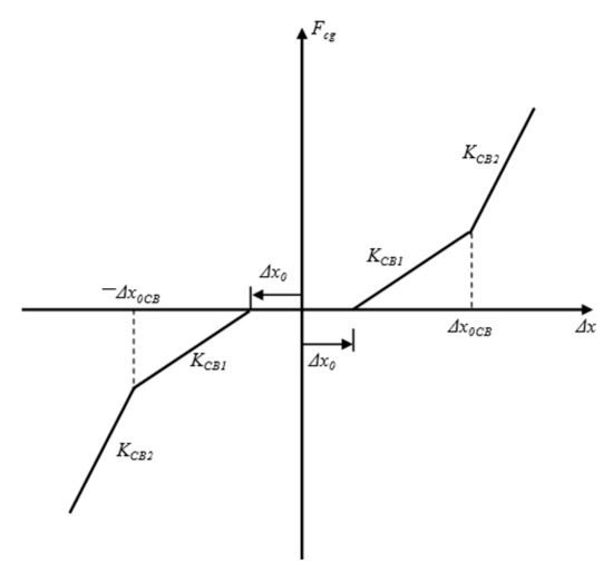
Figure 4. Schematic diagram of the nonlinear stiffness of coupler draft gear.

2.2.2. Longitudinal Vibration Absorption Device

This paper simplifies the longitudinal vibration absorption device as a damper hinged to the edges of the bases at the ends of adjacent vehicle bodies. Similar to coupler draft gear, it is only capable of axial elongation and compression, and the damping force is generated through differential axial velocities at its ends. Additionally, the nonlinear damping characteristics of the device are considered in this study, as depicted in Figure 5. The damping force F_CDL(R) can be represented by Equation (3).

$$F_{CDL\left(R\right)}=\{\begin{array}{ll}{C}_{CD1}\Delta v_{L\left(R\right)}& |\Delta v_{L\left(R\right)}|<\Delta v_{0CD}\\ sign(\Delta v_{L\left(R\right)})[C_{CD1}\Delta v_{0CD}+C_{CD2}(|\Delta v_{L\left(R\right)}|-\Delta v_{0CD}\left)\right]& |\Delta v_{L\left(R\right)}|\ge \Delta v_{0CD}\end{array}$$

(3)

where Δv_L(R) and Δv_0CD, respectively, denote the axial velocity differences of the left (right) longitudinal vibration absorption device and unloading velocity. C_CD1 and C_CD2 are damping values corresponding to varying velocity differences, respectively.

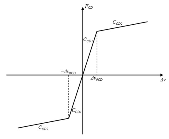
Figure 5. Schematic diagram of the nonlinear damping of the longitudinal vibration absorption device.

2.2.3. Tightly Sealed Windshield

To simulate interactions between neighboring vehicle bodies induced by windshield, three translational stiffness parameters ($k_{wdx}$, $k_{wdy}$, $k_{wdz}$) and three rotational stiffness parameters ($k_{wdrx}$, $k_{wdry}$, $k_{wdrz}$) are defined between the geometric centers of windshield. As a result, Equations (4) and (5) can be respectively used to calculate the forces and torques that the windshield exerts on the front end of the (n + 1)th vehicle body. According to Newton’s third law, the load applied on the rear end of the nth vehicle body can also be obtained.

$$\left\{\begin{array}{l}{F}_{wdxf}=k_{wdx}\left(x_{\left(n+1\right)wd}-x_{nwd}\right)\hfill \\ F_{wdyf}=k_{wdy}\left(y_{\left(n+1\right)wd}-y_{nwd}\right)\hfill \\ F_{wdzf}=k_{wdz}\left(z_{\left(n+1\right)wd}-z_{nwd}\right)\hfill \end{array}\right.$$

(4)

$$\left\{\begin{array}{l}{M}_{wdrxf}=k_{wdrx}\left({\varphi }_{\left(n+1\right)wd}-{\varphi }_{nwd}\right)\hfill \\ M_{wdryf}=k_{wdry}\left({\beta }_{\left(n+1\right)wd}-{\beta }_{nwd}\right)\hfill \\ M_{wdrzf}=k_{wdrz}\left({\psi }_{\left(n+1\right)wd}-{\psi }_{nwd}\right)\hfill \end{array}\right.$$

(5)

where ($x_{nwd}$, $y_{nwd}$, $z_{nwd}$, ${\varphi }_{nwd}$, ${\beta }_{nwd}$, ${\psi }_{nwd}$) and ($x_{\left(n+1\right)wd}$, $y_{\left(n+1\right)wd}$, $z_{\left(n+1\right)wd}$, ${\varphi }_{\left(n+1\right)wd}$, ${\beta }_{\left(n+1\right)wd}$, ${\psi }_{\left(n+1\right)wd}$) are displacements of 6 DOFs measured at the geometric centers of windshield at the rear end of the nth vehicle body and the front end of the (n + 1)th vehicle body, respectively.

Therefore, taking the inter-carriage coupling into account, each vehicle’s motion equations within the train subsystem can be written in matrix form using Equation (6).

$$M_v{\ddot{U}}_v+C_v{\dot{U}}_v+K_v{U}_v=F_v$$

(6)

The subscript ‘v’ in Equation (6) represents the first letter of ‘vehicle’, denoting a single vehicle in a train. The mass, damping, and stiffness matrices of a single vehicle in the global coordinate system are denoted by $M_v$, $C_v$, and $K_v$, respectively, and all of these matrices are symmetric. The acceleration, velocity, and displacement vectors of a single vehicle are represented by ${\ddot{U}}_v$, ${\dot{U}}_v$, and $U_v$, respectively. The applied loads on a single railway vehicle, such as gravity and wheel–rail interaction forces, are represented by the load vector $F_v$.

2.3. Track Subsystem

The functions of the track subsystem are supporting the train subsystem and guaranteeing safe train operations. During train operations, stresses and vibration energy resulting from wheel–rail contacts are conveyed through the track subsystem. The track subsystem’s mechanical and physical properties dictate the dynamic responses’ attenuation features and propagation efficiency. On the other hand, the track subsystem’s characteristics, such as its smoothness and stiffness, have a big impact on the dynamic behaviors of the train subsystem. Furthermore, seismic ground motions affect dynamic behaviors of train subsystems through track subsystems.

In this section, a twin-block ballastless track consisting of rails, fasteners, sleepers, track slabs, and a concrete support layer is established. Figure 6 and Figure 7 display the side and end views of the track subsystem, respectively.

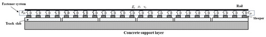
Figure 6. Side view of the track subsystem.

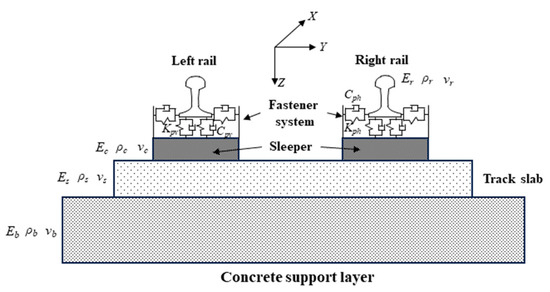
Figure 7. End view of the track subsystem.

The detailed descriptions and specific values of physical quantities depicted in Figure 6 and Figure 7 are provided in Table A2. The rail in this study is assumed to be an Euler beam on discrete point supports. Based on the theory of elastic beam vibrations and mode superposition method, differential equations governing the rail’s lateral, vertical, and torsional vibrations are presented from Equations (7)–(9).

$${\ddot{q}}_{Vk}\left(t\right)+\frac{E_r{I}_Y}{m_r}{\left(\frac{k\pi }{l}\right)}^4{q}_{Vk}\left(t\right)=-{\displaystyle \sum _{i=1}^N{F}_{Vi}{Z}_k\left(x_{si}\right)+{\displaystyle \sum _{m=1}^n{\displaystyle \sum _{j=1}^4{P}_{m,j}\left(t\right)Z_k\left(x_{m,j}\right)}}}\left(k=1~N_V\right)$$

(7)

$${\ddot{q}}_{Lk}\left(t\right)+\frac{E_r{I}_Z}{m_r}{\left(\frac{k\pi }{l}\right)}^4{q}_{Lk}\left(t\right)=-{\displaystyle \sum _{i=1}^N{F}_{Li}{Y}_k\left(x_{si}\right)+{\displaystyle \sum _{m=1}^n{\displaystyle \sum _{j=1}^4{Q}_{m,j}\left(t\right)Y_k\left(x_{m,j}\right)}}}\left(k=1~N_L\right)$$

(8)

$${\ddot{q}}_{Tk}\left(t\right)+\frac{G_r{I}_t}{{\rho }_r{I}_0}{\left(\frac{k\pi }{l}\right)}^2{q}_{Tk}\left(t\right)=-{\displaystyle \sum _{i=1}^N{M}_{si}{\Theta }_k\left(x_{si}\right)+{\displaystyle \sum _{m=1}^n{\displaystyle \sum _{j=1}^4{M}_{m,j}\left(t\right) {\Theta }_k\left(x_{m,j}\right)}}}\left(k=1~N_T\right)$$

(9)

where $I_Y$ and $I_Z$, respectively, stand for the moment of inertia of rail cross-section about y-axis and z-axis (the direction of y-axis and z-axis can be referred to in Figure 7). The torsional moment of inertia of rail cross-section is indicated by $I_t$, while the polar moment of inertia is indicated by $I_0$; $E_r$ and $G_r$ denotes elastic modulus and shear modulus of rail, respectively; and $m_r$ and ${\rho }_r$ represent rail’s mass per unit length and density. N and n are symbols for the number of fasteners per single rail and carriage. Subscripts $i$, $j$, and $m$ denote the ID of fastener ($i\in \left[1,N\right]$), wheelset ($j\in \left[1,4\right]$), and vehicle ($m\in \left[1,n\right]$), respectively; $x_{m,j}$ and $x_i$ are $x$-coordinates of j-th wheelset of m-th vehicle and i-th fastener, respectively. $F_{Vi}$ and $F_{Li}$ are rail’s vertical and lateral support reactions generated by i-th fastener, respectively; $P_{m,j}$, $Q_{m,j}$, and $M_{m,j}$ are vertical force, lateral force, and torque, respectively, induced by the j-th wheelset of the m-th vehicle on the rail. The subscript k denotes the modal order; $q_{Vk}$, $q_{Lk}$, and $q_{Tk}$ are k-th order modal coordinates; $N_V$, $N_L$, and $N_T$ denote the highest order of the vertical, lateral, and torsional mode shapes, respectively; and $Z_k$, $Y_k$, and ${\Theta }_k$ correspond to the k-th order modal functions for rail’s vertical, lateral, and torsional vibrations. The specific expressions for $Z_k$, $Y_k$, and ${\Theta }_k$ are presented in Equations (10)–(12).

$$Z_k\left(x\right)=\sqrt{\frac{2}{m_{r}l}}\sin \frac{k\pi x}{l}$$

(10)

$$Y_k\left(x\right)=\sqrt{\frac{2}{m_{r}l}}\sin \frac{k\pi x}{l}$$

(11)

$${\Theta }_k\left(x\right)=\sqrt{\frac{2}{{\rho }_r{I}_{0}l}}\sin \frac{k\pi x}{l}$$

(12)

where l denotes rail length. It should be noted that since the rail is modeled as an Euler beam on discrete supports, both the Y-axis and Z-axis represent displacements within the rail’s cross-sectional plane. Therefore, from the perspective of mode shapes, the mode shape functions for $Y_k$ and $Z_k$ are identical.

The approach described above involves isolating the rail from the track subsystem and modeling it independently, with the solution based directly on the mode superposition method. To facilitate rapid computation, the differential equations of rail motion are expressed in matrix form, as presented in Equation (13).

$$M_r{\ddot{U}}_r+C_r{\dot{U}}_r+K_r{U}_r=F_r$$

(13)

In Equation (13), the subscript ‘r’ represents the initial letter of ‘rail’. ${\ddot{U}}_r$, ${\dot{U}}_r$, and $U_r$ represent the vectors of the second-order derivatives of modal coordinates, first-order derivatives of modal coordinates, and modal coordinates of the rail, respectively. The matrices $M_r$, $C_r$, $K_r$, and $F_r$ correspond to the rail’s mass, damping, stiffness matrices, and load vector in global coordinate system.

The remaining parts of the track subsystem are modeled by the finite element method (FEM), utilizing solid elements. According to finite element theory, the equations of motion for the remainder of the track subsystem can be written as Equation (14).

$$M_t{\ddot{U}}_t+C_t{\dot{U}}_t+K_t{U}_t=F^{rs}+F^p$$

(14)

where $M_t$, $C_t$, and $K_t$ correspond to track subsystem’s mass, damping, and stiffness matrices (excluding rails); ${\ddot{U}}_t$, ${\dot{U}}_t$ and $U_t$ represent acceleration, velocity, and displacement vector (excluding rails). $F^{rs}$ and $F^p$ respectively denote the forces exerted by fasteners and external boundary conditions.

2.4. Wheel–Rail Interaction

The wheel–rail normal force is calculated by the theory of Hertzian nonlinear elastic contact theory [23], as shown in Equation (15).

$$N\left(t\right)=\left\{\begin{array}{l}{\left[\frac{1}{G_{wr}}\delta Z\left(t\right)\right]}^{3/2}\hspace{1em}\hspace{1em}\left(\delta Z\left(t\right)>0\right)\hfill \\ 0\hspace{1em}\hspace{1em}\hspace{1em}\hspace{1em}\hspace{1em}\hspace{1em}\hspace{1em}\left(\delta Z\left(t\right)\le 0\right)\hfill \end{array}\right.$$

(15)

where $G_{wr}$ denotes the wheel–rail contact constant and $\delta Z\left(t\right)$ denotes the wheel–rail penetration along normal direction of the wheel–rail contact plane.

Wheel–rail tangential creep force is initially determined according to Kalker’s linear creep theory [24]. However, this theory only works in small spin or creep rate scenarios. In order to make the computations appropriate for any creep condition, the Shen’s theory [25] is applied for the nonlinear correction.

It should be emphasized that two types of wheel–rail interaction forces are both defined within a contact-spot coordinate system whose origin $O_{Rc}$ is at the wheel–rail contact ellipse center, with the $O_{Rc}{X}_{Rc}$ aligned with the wheelset’s forward direction, the $O_{Rc}{Z}_{Rc}$ parallel to the normal of the wheel–rail contact plane, and the direction of $O_{Rc}{Y}_{Rc}$ determined by the right-hand rule lying within the contact plane.

It is required to convert wheel–rail forces calculated above from the contact-spot coordinate system to the global coordinate system because the wheel–rail forces in the vehicle’s equations of motion presented in Equation (6) are defined in the global coordinate system. The conversion relationships between these two coordinate systems on the left and right sides, respectively, are given by Equations (16) and (17).

$$\left\{\begin{array}{c}\mathit{i}\\ \mathit{j}\\ \mathit{k}\end{array}\right\}={\left[\begin{array}{lll}\mathrm{c}\mathrm{o}\mathrm{s}{\psi }_w& \mathrm{s}\mathrm{i}\mathrm{n}{\psi }_w& 0\\ -\mathrm{c}\mathrm{o}\mathrm{s}({\delta }_L+{\varphi }_w)\mathrm{s}\mathrm{i}\mathrm{n}{\psi }_w& \mathrm{c}\mathrm{o}\mathrm{s}({\delta }_L+{\varphi }_w)\mathrm{c}\mathrm{o}\mathrm{s}{\psi }_w& \mathrm{s}\mathrm{i}\mathrm{n}({\delta }_L+{\varphi }_w)\\ \mathrm{s}\mathrm{i}\mathrm{n}({\delta }_L+{\varphi }_w)\mathrm{s}\mathrm{i}\mathrm{n}{\psi }_w& -\mathrm{s}\mathrm{i}\mathrm{n}({\delta }_L+{\varphi }_w)\mathrm{c}\mathrm{o}\mathrm{s}{\psi }_w& \mathrm{c}\mathrm{o}\mathrm{s}({\delta }_L+{\varphi }_w)\end{array}\right]}^{-1}\left\{\begin{array}{l}{\mathit{i}}_{\mathit{L}\mathit{c}}\\ {\mathit{j}}_{\mathit{L}\mathit{c}}\\ {\mathit{k}}_{\mathit{L}\mathit{c}}\end{array}\right\}$$

(16)

$$\left\{\begin{array}{c}\mathit{i}\\ \mathit{j}\\ \mathit{k}\end{array}\right\}={\left[\begin{array}{lll}\mathrm{c}\mathrm{o}\mathrm{s}{\psi }_w& \mathrm{s}\mathrm{i}\mathrm{n}{\psi }_w& 0\\ -\mathrm{c}\mathrm{o}\mathrm{s}({\delta }_R-{\varphi }_w)\mathrm{s}\mathrm{i}\mathrm{n}{\psi }_w& \mathrm{c}\mathrm{o}\mathrm{s}({\delta }_R-{\varphi }_w)\mathrm{c}\mathrm{o}\mathrm{s}{\psi }_w& -\mathrm{s}\mathrm{i}\mathrm{n}({\delta }_R-{\varphi }_w)\\ -\mathrm{s}\mathrm{i}\mathrm{n}({\delta }_R-{\varphi }_w)\mathrm{s}\mathrm{i}\mathrm{n}{\psi }_w& \mathrm{s}\mathrm{i}\mathrm{n}({\delta }_R-{\varphi }_w)\mathrm{c}\mathrm{o}\mathrm{s}{\psi }_w& \mathrm{c}\mathrm{o}\mathrm{s}({\delta }_R-{\varphi }_w)\end{array}\right]}^{-1}\left\{\begin{array}{l}{\mathit{i}}_{\mathit{R}\mathit{c}}\\ {\mathit{j}}_{\mathit{R}\mathit{c}}\\ {\mathit{k}}_{\mathit{R}\mathit{c}}\end{array}\right\}$$

(17)

where the wheel–rail contact angle on the left and right sides is indicated by ${\delta }_L$ and ${\delta }_R$, respectively; ($i$, $j$, $k$), ($i_{Lc}$, $j_{Lc}$, $k_{Lc}$), and ($i_{Rc}$, $j_{Rc}$, $k_{Rc}$) are basis vectors in global coordinate system, left contact-spot coordinate system, and right contact-spot coordinate system, respectively.

2.5. Validation of Vehicle–Track Coupled Dynamics Model

Field testing is restricted to railway departments or institutions authorized by them in China; hence, conducting on-site tests is almost impractical. Additionally, the routine operation of the railway network would be disrupted by these experiments. Furthermore, regarding the data of on-site tests organized by the railway department, we are almost unable to access the mechanical parameters of trains and track structures, which means that the simulation parameters are incomplete and prevent us from using accurate parameters to replicate real circumstances. Thus, in this section, utilizing vehicle and track structure parameters listed in Table A1 and Table A2, the correctness of the established model in this study is verified from a numerical reliability standpoint. Assuming the ideal running conditions without considering track irregularities, the operating speed of the railway vehicle was set to 60 km/h. The time histories of wheel–rail vertical force as well as rail vertical acceleration and displacement are presented in Figure 8 and Figure 9, respectively.

Figure 8. Wheel–rail vertical force time history.

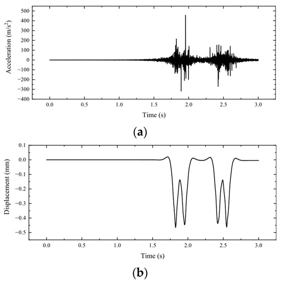
Figure 9. Rail vertical acceleration and displacement time histories: (a) rail vertical acceleration and (b) rail vertical displacement.

Based on Table A1, the train’s static axle load is roughly 57.2 kN. Under absolutely ideal operating conditions, the wheel–rail vertical force should oscillate around static axle load. Figure 8 illustrates, without any track irregularity disturbances, that the time history curve of wheel–rail vertical force stabilizes near 57.2 kN, with slight fluctuations in the initial segment attributed to simulation initialization. Meanwhile, the time history curves for rail vertical acceleration and displacement depicted in Figure 9 correspond with field-measured waveforms, indicating rail vibration status during the passage of a single-formation train [23,26,27]. Consequently, it can be considered that the model established in this study exhibits a certain level of accuracy and reliability.

2.6. Seismic Excitation

2.6.1. Selection of Seismic Ground Motion

Selecting appropriate seismic records as inputs for a vehicle/train–track coupled model is vital and essential. Many scholars, like Miyamoto [2,3,4], have employed simple harmonic motion as input for the wheel–rail coupled system to explore the operational safety and dynamic behaviors of trains under seismic conditions. However, the single frequency component of simple harmonic motion fails to capture the real dynamic responses of trains under seismic motions with multiple frequency components. This limitation restricts the depth of seismic analyses. Additionally, simple harmonic motion lacks the typical features of seismic motion, such as the rising segment, plateau, and descending segment compared with actual seismic motion records. In this paper, seismic motion selection according to the modal analysis of railway vehicles. The characteristic periods of the first 10 modes are presented in Table 2, indicating that the train subsystem is sensitive to low-frequency excitation. According to this, RSN3934 from the database of PEER is selected as the input of the coupled system, with acceleration time history and response spectrum along the east–west (EW) direction depicted in Figure 10. Its predominant period is 0.97 s.

Table 2. Train model’s characteristic periods of first 10-order modes.

Modal Order	Characteristic Period/s	Modal Order	Characteristic Period/s
1	1.4603	2	1.4520
3	0.9042	4	0.7064
5	0.6343	6	0.6151
7	0.5715	8	0.5691
9	0.2260	10	0.2260

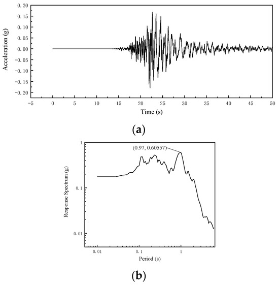
Figure 10. Acceleration time history and response spectrum of input seismic motion: (a) acceleration time history and (b) acceleration response spectrum.

2.6.2. Input Method of Seismic Ground Motion

By dividing the nodes of the track subsystem into support nodes and non-support nodes characterizing whether directly affected by seismic ground motion, Equation (14) can be rewritten into Equation (18).

$$\left[\begin{array}{ll}{\mathit{M}}_{\mathit{t}\mathit{t}}& {\mathit{M}}_{\mathit{t}\mathit{g}}\\ {\mathit{M}}_{\mathit{g}\mathit{t}}& {\mathit{M}}_{\mathit{g}\mathit{g}}\end{array}\right]\left[\begin{array}{l}{\ddot{\mathit{u}}}_{\mathit{t}}\\ {\ddot{\mathit{u}}}_{\mathit{g}}\end{array}\right]+\left[\begin{array}{ll}{\mathit{C}}_{\mathit{t}\mathit{t}}& {\mathit{C}}_{\mathit{t}\mathit{g}}\\ {\mathit{C}}_{\mathit{g}\mathit{t}}& {\mathit{C}}_{\mathit{g}\mathit{g}}\end{array}\right]\left[\begin{array}{l}{\dot{\mathit{u}}}_{\mathit{t}}\\ {\dot{\mathit{u}}}_{\mathit{g}}\end{array}\right]+\left[\begin{array}{ll}{\mathit{K}}_{\mathit{t}\mathit{t}}& {\mathit{K}}_{\mathit{t}\mathit{g}}\\ {\mathit{K}}_{\mathit{g}\mathit{t}}& {\mathit{K}}_{\mathit{g}\mathit{g}}\end{array}\right]\left[\begin{array}{l}{\mathit{u}}_{\mathit{t}}\\ {\mathit{u}}_{\mathit{g}}\end{array}\right]=\left[\begin{array}{l}{\mathit{F}}^{\mathit{r}\mathit{s}}\\ {\mathit{F}}^{\mathit{g}}\end{array}\right]$$

(18)

where subscripts “g” and “t” represent support nodes and non-support nodes. $F_g$ is the force vector applied on the track subsystem due to seismic excitations. The meaning of other physical quantities can be referenced in Equation (14). By expanding Equations (18) and (19) can be obtained.

$$\{\begin{array}{l}{\mathit{M}}_{\mathit{t}\mathit{t}}{\ddot{\mathit{u}}}_{\mathit{t}}+{\mathit{C}}_{\mathit{t}\mathit{t}}{\dot{\mathit{u}}}_{\mathit{t}}+{\mathit{K}}_{\mathit{t}\mathit{t}}{\mathit{u}}_{\mathit{t}}={\mathit{F}}_{\mathit{r}\mathit{s}}-({\mathit{M}}_{\mathit{t}\mathit{g}}{\ddot{\mathit{u}}}_{\mathit{g}}+{\mathit{C}}_{\mathit{t}\mathit{g}}{\dot{\mathit{u}}}_{\mathit{g}}+{\mathit{K}}_{\mathit{t}\mathit{g}}{\mathit{u}}_{\mathit{g}})\\ {\mathit{M}}_{\mathit{g}\mathit{g}}{\ddot{\mathit{u}}}_{\mathit{g}}+{\mathit{C}}_{\mathit{g}\mathit{g}}{\dot{\mathit{u}}}_{\mathit{g}}+{\mathit{K}}_{\mathit{g}\mathit{g}}{\mathit{u}}_{\mathit{g}}={\mathit{F}}_{\mathit{g}}-({\mathit{M}}_{\mathit{g}\mathit{t}}{\ddot{\mathit{u}}}_{\mathit{t}}+{\mathit{C}}_{\mathit{g}\mathit{t}}{\dot{\mathit{u}}}_{\mathit{t}}+{\mathit{K}}_{\mathit{g}\mathit{t}}{\mathit{u}}_{\mathit{t}})\end{array}$$

(19)

Based on the seismic ground motion records, Equations (6), (13) and (14) can then be simultaneously solved to obtain the coupled system’s responses. Furthermore, because the equations of motion of this coupled system form a large-scaled nonlinear system, the equations in this study are therefore solved numerically using the Zhai method (developed by Zhai [28]). This explicit dynamic integration method is well-known for its accuracy and stability within critical step size and is useful for quickly and easily solving large-scale dynamic problems without the need for simultaneous equation solving. Figure 11 displays the flow chart of the numerical simulation.

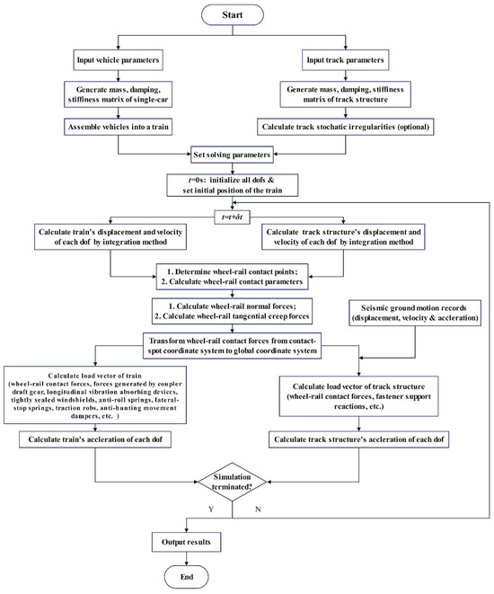
Figure 11. The flow chart of numerical simulation.

3. Result and Discussion

In this section, the variation patterns in the dynamic responses of vehicle/train–track coupled systems under non-uniform seismic motion conditions are investigated using four train models, namely, 1-car, 3-car, 5-car, and 8-car.

As illustrated in Figure 11, wheel–rail contact simulation is a primary factor that constrains the computational efficiency during analysis. The process of each increment step consists of a series of procedures for each wheelset on both sides, including searching wheel–rail contact points, calculating contact parameters (contact angle, radius of rolling circle, etc.), calculating wheel–rail interaction forces, and converting these wheel–rail interaction forces from wheel–rail contact-spot coordinate system to global coordinate system. Locating the wheel–rail contact points involves iterating over discretized points on the rail and tread profile, a process that is time-consuming. This comprehensive procedure contributes to a decrease in computational speed as the number of vehicles increases. Based on the variation patterns of train formation, in order to conserve computational resources and costs while ensuring simulation accuracy, it is necessary to investigate whether fewer railway vehicles in the numerical simulation can achieve the same requirements of the actual standard train formation model. Therefore, this section also aims to explore the optimal number of vehicles for numerical simulation under non-uniform seismic motions. In addition, in China and many countries with high-speed railways, a standard EMU high-speed train often consists of eight cars. Hence, the results from a complete 8-car standard formation serve as a benchmark for assessing the reliability and precision of the computational results from other train formations.

Besides, to mitigate the potential disturbances from random effects in the vehicle/train–track coupled system that could affect the numerical solutions and considering the high operational speed and large curve radii of high-speed railway, this study simulates ideal operational conditions. It means high-speed trains are modeled to run on smooth, straight-track structures at a consistent speed of 250 km/h. The train parameters are modeled after the Chinese CRH380B type ‘Harmony’ high-speed EMU train, while the track model is according to the CRTII type ballastless track system. The relevant parameters for the train and track subsystem are listed in Table A1 and Table A2.

3.1. Wheel–Rail Interaction Indices

In this subsection, the influences of train formation on dynamic behaviors and operational safety of high-speed trains from the viewpoint of wheel–rail interactions are investigated under non-uniform seismic motion conditions. This involves a detailed examination of how variations in train formation affect wheel–rail interaction indices, including wheel–rail lateral force, wheel–rail vertical force, derailment coefficient, and offload factor. The derailment coefficient is defined as the ratio of lateral to vertical wheel–rail force at a single contact point, while the offload factor measures the reduction in wheel load on one side relative to the static load. Both indices are essential for a thorough assessment of the operating safety of trains. The seismic record, as depicted in Figure 10, is modulated to intensities of 100 gal and 400 gal, respectively. Two modulated seismic ground motions are input horizontally (horizontal direction orthogonal to the railway track subsystem) into the train/vehicle–track coupled dynamics system as wave motions with an apparent velocity of 600 m/s, assuming that the direction of seismic wave propagation is opposite to the train’s running direction. Table 3 and Table 4 respectively list the peak values and relative errors of these four wheel–rail interaction indices for different train formations under two intensity levels of seismic ground motions. Meanwhile, to visually demonstrate the trends in these four indices, Figure 12 and Figure 13 depict the peak value trends of each index under two intensity levels of seismic ground motions, with the absolute values of relative errors presented in the form of bar charts.

Table 3. Wheel–rail interaction peak values and relative errors of different kinds of train formations (PGA = 100 gal).

	Lateral Force		Vertical Force		Derailment Coefficient		Offload Factor
Train Formation	Peak Value/kN	Relative Error	Peak Value/kN	Relative Error	Peak Value	Relative Error	Peak Value	Relative Error
1	16.672	−4.81%	104.380	0.62%	0.348	−8.42%	0.595	5.31%
3	14.369	−17.96%	106.053	2.23%	0.266	−30.00%	0.587	3.89%
5	17.200	−1.79%	102.775	−0.93%	0.371	−2.37%	0.549	−2.83%
8	17.514	0.00%	103.737	0.00%	0.380	0.00%	0.565	0.00%

Table 4. Wheel–rail interaction peak values and relative errors of different kinds of train formations (PGA = 400 gal).

	Lateral Force		Vertical Force		Derailment Coefficient		Offload Factor
Train Formation	Peak Value/kN	Relative Error	Peak Value/kN	Relative Error	Peak Value	Relative Error	Peak Value	Relative Error
1	33.146	−12.54%	117.369	−4.20%	0.698	−5.42%	0.717	−5.53%
3	51.524	35.95%	120.114	−1.96%	1.163	57.59%	0.699	−7.91%
5	38.969	2.83%	121.392	−0.92%	0.766	3.79%	0.746	−1.71%
8	37.898	0.00%	122.515	0.00%	0.738	0.00%	0.759	0.00%

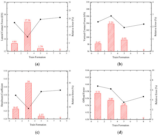
Figure 12. Variation trend of wheel–rail interaction indices’ peak values and relative errors versus train formations (PGA = 100 gal): (a) wheel–rail lateral force; (b) wheel–rail vertical force; (c) derailment coefficient; and (d) offload factor.

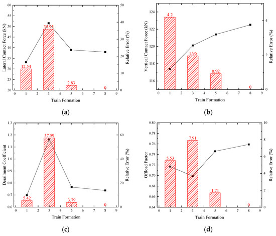
Figure 13. Variation trend of wheel–rail interaction indices’ peak values and relative errors versus train formations (PGA = 400 gal): (a) wheel–rail lateral force; (b) wheel–rail vertical force; (c) derailment coefficient; and (d) offload factor.

Table 3 and Table 4 and Figure 12 and Figure 13 show that compared to the simulation results of the standard 8-car train formation model, the relative errors of the wheel–rail interaction indices for the 5-car formation are noticeably smaller than those for the single-car and 3-car configurations and are very close to those of the 8-car formation. When the input seismic acceleration peak value is 100 gal, the relative errors for wheel–rail lateral force, wheel–rail vertical force, derailment coefficient, and offload factor are −1.79%, −0.93%, −2.37%, and −2.83%, respectively; when the seismic acceleration peak value is adjusted to 400 gal, the relative errors for these four indices are 2.83%, −0.92%, 3.79%, and −1.71%, respectively. These results indicate that the 5-car formation maintains high simulation accuracy, and the relative errors under both seismic conditions do not exceed 5%, making it a viable alternative to the 8-car formation for analyzing the dynamic responses and operational safety of trains under non-uniform seismic actions.

In contrast, the numerical solutions of the 3-car formation model exhibit significant deviations from those of 8-car formation, indicating poor simulation accuracy. For seismic input with a peak acceleration of 100 gal, the relative errors in wheel–rail lateral force and derailment coefficient are −17.96% and −30%, respectively, while for a peak acceleration of 400 gal, these errors increase to 35.95% and 57.59%. Not only are the relative errors large, but the results also show instability. The wheel–rail interaction indices are significantly underestimated when peak acceleration is equal to 100 gal and overestimated when peak acceleration is equal to 400 gal, rendering the 3-car formation model unsuitable for analyzing the operational safety of trains.

The results also indicate that although the wheel–rail interaction indices for the single-car model exhibit larger errors compared to those of the 5-car formation, they are substantially lower than those obtained in the 3-car formation model. Consequently, the single-car model can still meet accuracy needs for rough qualitative analysis and offers advantages in computational speed compared to the 5-car model, facilitating rapid and preliminary assessments of train operational safety and wheel–rail interactions prior to more detailed quantitative analysis. Additionally, it should be noted that relative to the 8-car standard formation, the wheel–rail interaction indices for the single-car model are comparatively smaller. This may be due to the interactions between adjacent vehicles, which tends to amplify wheel–rail interactions. Furthermore, the train with multi-car formation allows the track subsystem to receive more energy through wheel–rail contact interfaces simultaneously, leading to more pronounced dynamic responses in the track structure. This effect is compounded by dynamic feedback and coupling mechanisms between the train and track, intensifying the train’s dynamic responses and, consequently, the severity of wheel–rail interactions. Specifically, for seismic inputs with a peak acceleration of 100 gal, where the seismic intensity is lower, the interaction indices of the single-car model are slightly greater than those of the 8-car formation model. However, with inputs at a peak acceleration of 400 gal, the wheel–rail lateral force, wheel–rail vertical force, derailment coefficient, and offload factor are all lower than those of the 8-car formation model, with relative errors of −12.54%, −4.20%, −5.42%, and −5.53%, respectively.

3.2. Vehicle Kinematic Indices

This subsection primarily investigates the influences of train formation on the dynamic responses and operational safety of trains under non-uniform seismic excitation from the perspective of vehicle kinematic indices. In accordance with current railway standards, the vehicle body’s dynamic response is a pivotal criterion for assessing the operational safety. Table 5 and Table 6 present the peak values and relative errors of lateral and vertical accelerations of vehicle bodies for various train–track coupled dynamic models with different kinds of train formations under two levels of input seismic acceleration, along with several other degrees of freedom of the vehicle bodies for supplementary evaluation. Additionally, to visually demonstrate the variation trends of displacement or acceleration for each degree of freedom, Figure 14 and Figure 15 depict the peak value trends of each index under two levels of seismic intensity, with the absolute values of relative errors presented in bar chart form.

Table 5. Peak values and relative errors of dynamic responses of vehicle bodies (PGA = 100 gal).

	Lateral Acceleration		Vertical Acceleration		Yaw Angle		Yaw Angular Acceleration		Roll Angle		Roll Angular Acceleration
Train Formation	Peak Value /(m/s2)	Relative Error	Peak Value /(m/s2)	Relative Error	Peak Value /Rad	Relative Error	Peak Value /(Rad/s2)	Relative Error	Peak Value /Rad	Relative Error	Peak Value /(Rad/s2)	Relative Error
1	0.430	−24.83%	0.0313	44.91%	9.754 × 10−4	59.82%	0.0429	32.41%	0.0146	0.69%	0.391	−4.63%
3	0.554	−3.15%	0.0233	7.87%	7.908 × 10−4	29.58%	0.0266	−17.90%	0.0148	2.07%	0.397	−3.17%
5	0.587	2.62%	0.0210	−2.78%	6.046 × 10−4	−0.93%	0.0311	−4.01%	0.0139	−4.14%	0.411	0.24%
8	0.572	0.00%	0.0216	0.00%	6.103 × 10−4	0.00%	0.0324	0.00%	0.0145	0.00%	0.410	0.00%

Table 6. Peak values and relative errors of dynamic responses of vehicle bodies (PGA = 400 gal).

	Lateral Acceleration		Vertical Acceleration		Yaw Angle		Yaw Angular Acceleration		Roll Angle		Roll Angular Acceleration
Train Formation	Peak Value /(m/s2)	Relative Error	Peak Value /(m/s2)	Relative Error	Peak Value /Rad	Relative Error	Peak Value /(Rad/s2)	Relative Error	Peak Value /Rad	Relative Error	Peak Value /(Rad/s2)	Relative Error
1	2.483	−7.04%	0.0986	−9.54%	1.120 × 10−3	−1.32%	0.0565	9.71%	0.0738	−2.25%	2.173	−2.12%
3	2.470	−7.53%	0.0920	−15.60%	8.899 × 10−4	−21.59%	0.0349	−32.23%	0.0695	−7.95%	2.029	−8.60%
5	2.705	1.27%	0.1040	−4.59%	1.080 × 10−3	−4.85%	0.0495	−3.88%	0.0743	−1.59%	2.245	1.13%
8	2.671	0.00%	0.1090	0.00%	1.135 × 10−3	0.00%	0.0515	0.00%	0.0755	0.00%	2.220	0.00%

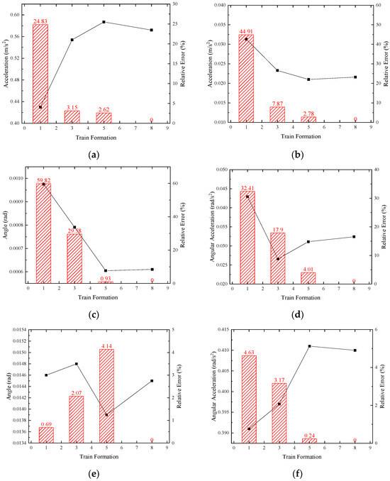
Figure 14. Trends in peak values of vehicle body degrees of freedom versus different train formations (PGA = 100 gal): (a) lateral acceleration; (b) heave acceleration; (c) yaw angle; (d) yaw angular acceleration; (e) roll angle; and (f) roll angular acceleration.

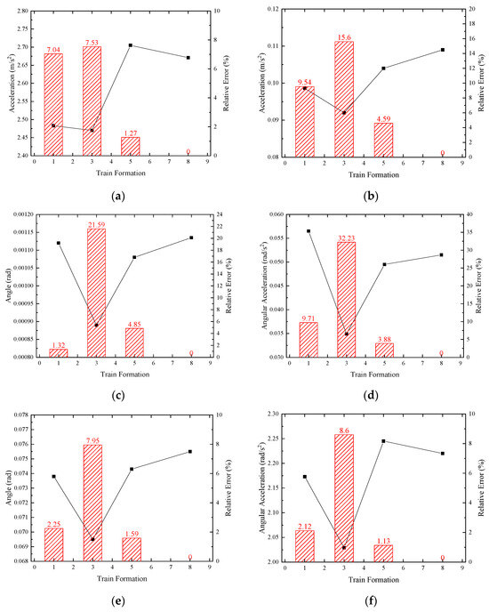
Figure 15. Trends in peak values of vehicle body degrees of freedom versus different train formations (PGA = 400 gal): (a) lateral acceleration; (b) heave acceleration; (c) yaw angle; (d) yaw angular acceleration; (e) roll angle; and (f) roll angular acceleration.

From Table 5 and Table 6 and Figure 14 and Figure 15, it is evident that the dynamic responses of the vehicle bodies exhibit significant variations with changes in train formation when considering seismic wave propagation effects.

For the single-car model, as detailed in Section 3.1, it can generally meet the accuracy requirements for rough qualitative analysis under non-uniform seismic input conditions. However, as shown in Table 5 and Table 6, the accuracy of dynamic responses of car bodies is poor for the single-car model, with relative errors in peak values of lateral acceleration of −24.83% and −7.04%. This substantial discrepancy is primarily due to the absence of inter-carriage connection devices in the single-car formation model, resulting in markedly different dynamic responses compared to the 8-car and 5-car formation models.

Figure 16 illustrates the time history curves of vehicle bodies’ lateral acceleration for single-car models and 8-car models (front, middle, and rear cars) under seismic motions with two distinct acceleration amplitudes, along with their corresponding Fourier amplitude spectra, and the differences in peak values are highlighted in Figure 16a,b. Additionally, the single-car model does not capture the distribution characteristics of dynamic responses observed in multi-car formations. As shown in Figure 16a, under a seismic acceleration peak of 100 gal, the lateral acceleration of the middle car in the 8-car formation model is substantially lower than that of the front and rear cars, particularly the front one. The Fourier amplitude spectrum in Figure 16c within the dominant frequency range (0.5~2 Hz) further demonstrates that the amplitude at the front car significantly exceeds that of the middle cars. This disparity diminishes as the input acceleration increases, leading to the middle car’s lateral acceleration converging towards that of the front and rear cars, as depicted in Figure 16b. When input acceleration is equal to 400 gal, as shown in Figure 16d, amplitude values across all frequency components are more consistent, except in the low-frequency band (below 1 Hz), where the front car’s amplitude is notably higher than those of the middle cars. Similar trends are observed in the vertical, pitch, and also those for other train formation models. Thus, compared to single-car models, multi-car train models can more accurately simulate the distribution characteristics of train dynamic responses. Detailed consideration of inter-carriage connection devices enables a more precise simulation of the lateral and vertical dynamic behaviors of high-speed trains’ vehicle bodies, enhancing modeling accuracy and reliability.

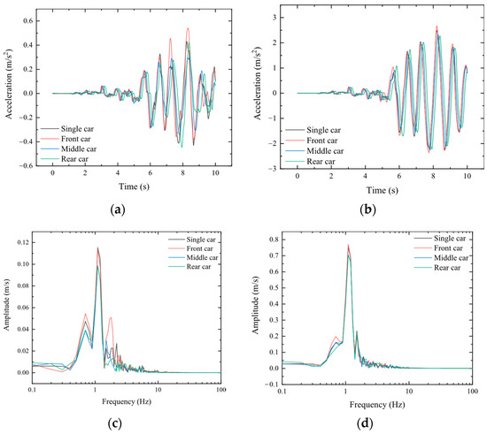
Figure 16. Comparison of vehicle bodies’ lateral acceleration time histories and Fourier amplitude spectra between 1-vehicle model and 8-vehicle model: (a) lateral acceleration (PGA = 100 gal); (b) lateral acceleration (PGA = 400 gal); (c) Fourier amplitude spectrum of lateral acceleration (PGA = 100 gal); and (d) Fourier amplitude spectrum of lateral acceleration (PGA = 400 gal).

The 5-car formation model exhibits high accuracy, with relative errors significantly smaller than those of single-car and 3-car formation models, all below 5%. Specifically, for seismic inputs with a peak acceleration of 100 gal, the relative errors in lateral and vertical accelerations of the vehicle body are 2.62% and −2.78%, respectively. When the peak acceleration is 400 gal, the relative errors are 1.27% and −4.59%, respectively. Therefore, from the perspective of vehicle kinematics and considering non-uniform seismic ground motion conditions, opting for a 5-car formation model over an 8-car formation model for numerical simulations could be advantageous to enhance computational efficiency while maintaining simulation accuracy.

4. Conclusions

This study investigates the influences of train formation on the dynamic responses and operational safety of high-speed trains under non-uniform seismic ground motion from various viewpoints through the development of a comprehensive vehicle/train–track coupled dynamics model. Based on this, the study also aims to explore the optimal train formation by balancing computing efficiency and simulation accuracy when using an 8-car formation as a benchmark, considering a standard EMU high-speed train often consists of eight cars in China and many other countries with high-speed railways. To eliminate the effects of random disturbances on simulation patterns, this study does not consider track stochastic irregularities, assuming the trains operate on a straight, smooth, ideal track structure. The conclusions are as follows:

(1) The use of a 5-car formation model yields superior computational results. Compared to the 8-car formation model, it achieves high computational precision with relative errors below 5% in both wheel–rail interaction and vehicle dynamic responses. Therefore, substituting an 8-car formation with a 5-car formation model in numerical simulations satisfies the accuracy requirements under consideration of seismic wave propagation effects while significantly enhancing computational efficiency and saving resources. Specifically, the 5-car formation model can save approximately one-third of the simulation time compared to the 8-car formation model.

(2) Although the single-car formation model presents a relatively larger error from the perspective of wheel–rail interaction compared to the 5-car formation model, it still performs better than the 3-car formation model. Therefore, the single-car formation model is suitable for rough qualitative analysis of train operational safety and offers advantages in computational speed, facilitating a quick, preliminary qualitative evaluation of train running safety and wheel–rail interaction levels prior to more detailed quantitative analysis. However, in terms of vehicle dynamic response, the single-car model exhibits a larger relative error compared to the 8-car formation model. Thus, if the focus is on wheel–rail interaction levels, the single-car model is suitable for qualitative analysis.–

(3) The 3-car formation model, regardless of whether it is evaluated from the perspective of wheel–rail interaction or vehicle dynamic response, exhibits large relative errors and fails to meet the requirements for computational accuracy. Therefore, the use of a 3-car formation model is not recommended when considering seismic wave propagation effects.

(4) Considering inter-carriage connection devices highlights distinct distribution characteristics of trains’ dynamic responses, where the middle car bodies show smaller dynamic responses compared to the front and rear cars. Furthermore, this distribution characteristic diminishes as the intensity of the seismic ground motion increases. Therefore, employing a multi-car formation model can provide a more precise simulation of the train bodies’ lateral and vertical dynamic behaviors, enhancing the accuracy and reliability of the modeling.

References

- Zhao, H.; Wei, B.; Jiang, L.; Xiang, P.; Zhang, X.; Ma, H.; Xu, S.; Wang, L.; Wu, H.; Xie, X. A Velocity-Related Running Safety Assessment Index in Seismic Design for Railway Bridge. Mech. Syst. Signal Process. 2023, 198, 110305. [Google Scholar] [CrossRef]
- Miyamoto, T.; Matsumoto, N.; Sogabe, M.; Shimomura, T.; Nishiyama, Y.; Matsuo, M. Full-Scale Experiment on the Dynamic Behavior of Railway Vehicles against Heavy Track Vibration. J. Environ. Eng. 2007, 2, 419–428. [Google Scholar] [CrossRef]
- Miyamoto, T.; Ishida, H. Numerical Analysis Focusing on the Running Safety of an Improved Bogie during Seismic Vibration. Q. Rep. RTRI 2008, 49, 173–177. [Google Scholar] [CrossRef][Green Version]
- Iida, K.; Suzuki, M.; Miyamoto, T.; Nishiyama, Y.; Nakajima, D.; Kajitani, Y. Development of a Lateral Damper to Improve the Running Safety of Railway Vehicles during an Earthquake. Q. Rep. RTRI 2012, 53, 34–40. [Google Scholar] [CrossRef]
- Nishimura, K.; Terumichi, Y.; Morimura, T.; Adachi, M.; Morishita, Y.; Miwa, M. Using Full Scale Experiments to Verify a Simulation Used to Analyze the Safety of Rail Vehicles During Large Earthquakes. J. Comput. Nonlinear Dyn. 2015, 10, 031013. [Google Scholar] [CrossRef]
- Ju, S.H.; Li, H.C. Dynamic Interaction Analysis of Trains Moving on Embankments during Earthquakes. J. Sound Vib. 2011, 330, 5322–5332. [Google Scholar] [CrossRef]
- Yang, X.; Wang, H.; Jin, X. Numerical Analysis of a Train-Bridge System Subjected to Earthquake and Running Safety Evaluation of Moving Train. Shock Vib. 2016, 2016, 9027054. [Google Scholar] [CrossRef]
- Cheng, Y.-C.; Chen, C.-H.; Hsu, C.-T. Derailment and Dynamic Analysis of Tilting Railway Vehicles Moving Over Irregular Tracks Under Environment Forces. Int. J. Struct. Stab. Dyn. 2017, 17, 1750098. [Google Scholar] [CrossRef]
- Zeng, Q.; Dimitrakopoulos, E.G. Seismic Response Analysis of an Interacting Curved Bridge–Train System under Frequent Earthquakes. Earthq. Eng. Struct. Dyn. 2016, 45, 1129–1148. [Google Scholar] [CrossRef]
- Tanabe, M.; Goto, K.; Watanabe, T.; Sogabe, M.; Wakui, H.; Tanabe, Y. A Simple and Efficient Numerical Model for Dynamic Interaction of High Speed Train and Railway Structure Including Derailment during an Earthquake. Procedia Eng. 2017, 199, 2729–2734. [Google Scholar] [CrossRef]
- Chen, L.-K.; Kurtulus, A.; Dong, Y.-F.; Taciroglu, E.; Jiang, L.-Z. Velocity Pulse Effects of Near-Fault Earthquakes on a High-Speed Railway Vehicle-Ballastless Track-Benchmark Bridge System. Veh. Syst. Dyn. 2022, 60, 2963–2987. [Google Scholar] [CrossRef]
- Zhou, T.; Jiang, L.; Liu, X.; Xiang, P.; Lai, Z.; Zhang, Y. An Efficient Simplified Model for High-Speed Railway Simply Supported Bridge under Earthquakes. Struct. Infrastruct. Eng. 2022, 19, 1811–1825. [Google Scholar] [CrossRef]
- Zhou, T.; Jiang, L.; Liu, X.; Xiang, P.; Lai, Z. Running Safety of High-Speed Railway Vehicles on the Elastoplastic Track-Subgrade-Bridge System under near-Fault Pulse-Type Earthquakes. Eng. Struct. 2023, 280, 115692. [Google Scholar] [CrossRef]
- Zhou, T.; Jiang, L.; Xiang, P.; Liu, X. Effects of Near-Fault Pulse-Type Ground Motion on Train–Track–Bridge Coupled System with Nonlinear Supports. Nonlinear Dyn. 2023, 111, 6213–6238. [Google Scholar] [CrossRef]
- Yu, J.; Zhou, W.; Jiang, L.; Peng, K.; Zu, L. Train Effect on the Vibration Behavior of High-Speed Railway Track-Bridge System Subjected to Seismic Excitation. Soil Dyn. Earthq. Eng. 2023, 172, 108049. [Google Scholar] [CrossRef]
- Jiang, L.; Peng, K.; Zhou, W.; Yu, J. Study on the Seismic Influence Coefficient of Track Irregularity on the Train Dynamic Effect of High-Speed Railway Bridge. Mech. Based Des. Struct. Mach. 2023, 52, 3339–3357. [Google Scholar] [CrossRef]
- Zhao, H.; Wei, B.; Guo, P.; Tan, J.; Xiang, P.; Jiang, L.; Fu, W.; Liu, X. Random Analysis of Train-Bridge Coupled System under Non-Uniform Ground Motion. Adv. Struct. Eng. 2023, 26, 1847–1865. [Google Scholar] [CrossRef]
- Fang, S.; Huang, R.; Guo, W.; He, C.; Jiang, L.; Yu, Z.; Wang, Y.; Zeng, C.; Liang, G.; Yang, S. Safety Speed Threshold of High-Speed Train Running on Bridges under Seismic Excitation of Different Soil Types. Structures 2023, 58, 105429. [Google Scholar] [CrossRef]
- ZHAI, W.M.; CAI, C.B.; GUO, S.Z. Coupling Model of Vertical and Lateral Vehicle/Track Interactions. Veh. Syst. Dyn. 1996, 26, 61–79. [Google Scholar] [CrossRef]
- Zeng, Z.-P.; Zhao, Y.-G.; Xu, W.-T.; Yu, Z.-W.; Chen, L.-K.; Lou, P. Random Vibration Analysis of Train–Bridge under Track Irregularities and Traveling Seismic Waves Using Train–Slab Track–Bridge Interaction Model. J. Sound Vib. 2015, 342, 22–43. [Google Scholar] [CrossRef]
- Ju, S.H.; Hung, S.J. Derailment of a Train Moving on Bridge during Earthquake Considering Soil Liquefaction. Soil Dyn. Earthq. Eng. 2019, 123, 185–192. [Google Scholar] [CrossRef]
- LING, L.; JIN, X. A 3D Model for Coupling Dynamics Analysis of High-Speed Train/Track System. J. Zhejiang Univ. Sci. A 2014, 15, 964–983. [Google Scholar] [CrossRef]
- Chen, Z.; Fang, H. An Alternative Solution of Train-Track Dynamic Interaction. Shock Vib. 2019, 2019, 1859261. [Google Scholar] [CrossRef]
- Kalker, J.J. Wheel-Rail Rolling Contact Theory. Wear 1991, 144, 243–261. [Google Scholar] [CrossRef]
- Shen, Z.Y.; Hedrick, J.K.; Elkins, J.A. A Comparison of Alternative Creep Force Models for Rail Vehicle Dynamic Analysis. Veh. Syst. Dyn. 1983, 12, 79–83. [Google Scholar] [CrossRef]
- Cui, X.; Chen, G.; Zhao, J.; Yan, W.; Ouyang, H.; Zhu, M. Field Investigation and Numerical Study of the Rail Corrugation Caused by Frictional Self-Excited Vibration. Wear 2017, 376–377, 1919–1929. [Google Scholar] [CrossRef]
- Zhu, Z.; Gong, W.; Wang, L.; Li, Q.; Bai, Y.; Yu, Z.; Harik, I.E. An Efficient Multi-Time-Step Method for Train-Track-Bridge Interaction. Comput. Struct. 2018, 196, 36–48. [Google Scholar] [CrossRef]
- Zhai, Wanming Two Simple Fast Integration Methods for Large-Scale Dynamic Problems in Engineering. Int. J. Numer. Methods Eng. 1996, 39, 4199–4214. [CrossRef]
Disclaimer/Publisher’s Note: The statements, opinions and data contained in all publications are solely those of the individual author(s) and contributor(s) and not of MDPI and/or the editor(s). MDPI and/or the editor(s) disclaim responsibility for any injury to people or property resulting from any ideas, methods, instructions or products referred to in the content. |
© 2024 by the authors. Licensee MDPI, Basel, Switzerland. This article is an open access article distributed under the terms and conditions of the Creative Commons Attribution (CC BY) license (https://creativecommons.org/licenses/by/4.0/).