Study on the Effect of Burial Depth on Selection of Optimal Intensity Measures for Advanced Fragility Analysis of Horseshoe-Shaped Tunnels in Soft Soil

Abstract

Seismic intensity measures (IMs) can directly affect the seismic risk assessment and the response characteristics of underground structures, especially when considering the key variable of burial depth. This means that the optimal seismic IMs must be selected to match the underground structure under different buried depth conditions. In the field of seismic engineering design, peak ground acceleration (PGA) is widely recognized as the optimal IM, especially in the seismic design code for aboveground structures. However, for the seismic evaluation of underground structures, the applicability and effectiveness still face certain doubts and discussions. In addition, the adverse effects of earthquakes on tunnels in soft soil are particularly prominent. This study aims to determine the optimal IMs applicable to different burial depths for horseshoe-shaped tunnels in soft soil using a nonlinear dynamic time history analysis method, and based on this, establish the seismic fragility curves that can accurately predict the probability of tunnel damage. The nonlinear finite element analysis model for the soil–tunnel interaction system was established. The effects of different burial depths on damage to horseshoe-shaped tunnels in soft soil were systematically studied. By adopting the incremental dynamic analysis (IDA) method and assessing the correlation, efficiency, practicality, and proficiency of the potential IMs, the optimal IMs were determined. The analysis indicates that PGA emerges as the optimal IM for shallow tunnels, whereas peak ground velocity (PGV) stands as the optimal IM for medium-depth tunnels. Furthermore, for deep tunnels, velocity spectral intensity (VSI) emerges as the optimal IM. Finally, the seismic fragility curves for horseshoe-shaped tunnels in soft soil were built. The proposed fragility curves can provide a quantitative tool for evaluating seismic disaster risk, and are of great significance for improving the overall seismic resistance and disaster resilience of society.

1. Introduction

Tunnel construction is one of the most important global public infrastructure construction projects, widely used in transportation and public utility networks. In order to cope with the increasing pressure of urban traffic, many coastal cities have begun to develop tunnel construction projects to meet the growing needs of urban development [1,2,3]. However, soft soil is commonly present in coastal cities, characterized by a loose structure, low shear strength, large deformation, and obvious soil stratification, which make the engineering geological environment relatively complex [4,5]. When an earthquake occurs, seismic vibration can cause the liquefaction of soft soil and make the soil lose its shear strength, resulting in the damage and collapse of the tunnel structure, which may cause serious casualties and economic losses [6,7,8]. As a result of the Hanshin earthquake that occurred in Japan in 1995, the world’s first subway station Daikai subway station totally collapsed [9]. The station was a box-shaped structure, and the earthquake caused almost complete collapse of the middle columns; the maximum settlement reached 2.5 m. In the 1999 Chichi earthquake in Taiwan, many tunnels were severely damaged [10]. The Wenchuan earthquake in China brought about extreme destruction to the Longxi, Longdongzi, and Zipingpu tunnels [11,12]. Ample evidence indicates that soft soil may have a great influence on tunnels, particularly those prone to high-intensity earthquakes. This may become the main obstacle to the normal operation of tunnels, which brings great challenges to tunnel engineering. Therefore, assessing the fragility and risk of tunnels in soft soil under various seismic conditions is essential for modern transportation construction, resilient and repairable design, and the safety assessment of new infrastructure.

IM is regarded as a link between the risk of earthquakes and the seismic response. Determining optimal IM can dramatically decrease the uncertainty in structural seismic demand prediction [13,14,15]. IM is the most significant parameter in fragility analysis [16]. Numerous studies indicate that IM is the important analytical parameter for seismic hazard analysis, earthquake engineering, and earthquake warning systems. Previous research has provided many reasonable suggestions for selecting seismic intensity measures for aboveground structures. IM is used to estimate the influence of earthquakes on buildings and assist engineers in structural design and evaluation. Researchers generally adopt single-parameter IM for aboveground buildings, which reflects amplitude characteristics [17]. Additionally, IM reflecting spectral characteristics is used [18]. There are IMs that reflect duration characteristics, namely the elastic response spectrum Sa(T) [19]. Other commonly used measures are cumulative absolute velocity (CAV) and Arias Intensity (AI), which reflect the cumulative effect of seismic motion [20]. Lin et al. [21] proposed the two-parameter SN1 and SN2, which are applicable to the effects of strong seismic actions caused by the nonlinear development of structures. The criteria for determining the optimal seismic intensity measure (IM) for structural fragility assessment include efficiency, practicality, correlation, and proficiency [22,23,24]. Khosravikia et al. [25] suggested that PGV can more accurately evaluate the seismic requirements of bridge structures. Heshmati and Jahangiri [26] investigated the various seismic responses of steel diagrid systems under large earthquakes and finally determined that the optimal IMs are PGV and the ratio between the peak ground velocity and the peak ground acceleration (PGV/PGA).

Considering the confining influence of soil, the damage characteristics exhibited by tunnels stand distinctively apart from those observed in aboveground building structures. At present, the research on the optimal IM of tunnels is very limited. Nguyen et al. [27] conducted nonlinear framework analysis and established fragility curves for underground structures. The results indicate that it is recommended to use PGV/V₃₀ as the optimal IM, rather than PGA and PGV. Chen et al. [28] studied the correlation between the damage measure and IM for underground structures in mountainous areas. The results show that a speed-related intensity measure can effectively reflect the overall damage degree of mountainous tunnels. Sun et al. [29,30] established a three-dimensional finite element model of deep buried hydraulic tunnels to carry out nonlinear dynamic time history analysis, selecting PGV and v_RMS as the optimal IMs among 15 tested IMs, which can predict the failure risk of deep buried hydraulic tunnels. Huang et al. [31,32] proposed the optimal IMs suitable for circular tunnels with different burial depths, putting forward that PGV and PGA are the optimal IMs for shallow and deep buried tunnels, respectively. Zhong et al. [33] studied the optimal seismic IMs suitable for shallow buried subway stations. Through comprehensive comparison, the PGA and PGV were determined as the optimal IMs. Zhuang et al. [34] studied the Dakai subway station and proposed peak relative lateral displacement (PRLD) and PGA as the IMs appropriate for estimating the seismic behavior of shallow structures.

Generally speaking, numerous factors influence the seismic performance of tunnels, such as seismic dynamics, geometry and size, material properties, ground water level, and soil conditions. Besides these, the buried depth of the tunnels is also one of the most important variables for fragility analysis. Most of the current research on tunnels focuses on fixed burial depth, but previous studies have highlighted the importance of considering changes in tunnel behavior under different burial depths [35,36,37,38,39]. In current research, there is no consensus on determining the optimal IMs in tunnels with different burial depths. With the development of the social economy and the continuous acceleration of urbanization, the utilization of urban land is becoming increasingly tense. In order to make full use of limited land resources, horseshoe-shaped tunnels have been widely used in urban construction due to the high utilization rate of underground space. Therefore, it is important to determine the optimal IMs for fragility analysis of horseshoe-shaped tunnels with different burial depths.

The fragility curve plays a prominent part in structural seismic evaluation. In recent years, the fragility curve has also been widely studied and developed. Argyroudis et al. [40] researched the fragility curve of shallow buried circular tunnels. Tsinidis et al. [41] conducted relevant experiments on centrifuges and vibration tables, providing a more detailed introduction to tunnel seismic analysis and fragility curves. According to previous research findings, a large number of achievements have been made in assessing the seismic responsiveness and fragility of underground structures with rectangular, circular, and bifurcated cross-sections [42,43,44,45]. However, due to limited research on the seismic fragility of horseshoe-shaped tunnels, there remains a significant lack of clarity on the identification of the optimal IMs for such structures.

This paper aims to determine the optimal IMs of horseshoe-shaped tunnels with different burial depths, and derive representative seismic fragility curves. The two-dimensional finite element numerical analysis model was established to comprehensively examine the soil–tunnel system interaction at different burial depths, and nonlinear dynamic time history analysis was conducted on typical horseshoe-shaped tunnels. The influence of different burial depths on the seismic response characteristics, especially the damage characteristics of horseshoe-shaped tunnels, was studied. Seventeen selected IMs were examined in accordance with four different criteria. The comprehensive comparative analysis of commonly used seismic IMs was performed, then the optimal IM applicable to horseshoe-shaped tunnels with different buried depths was determined. In addition, seismic fragility curves for typical tunnels were developed.

2. Theory and Formula of Seismic Fragility Analysis

2.1. Basic Theory

Seismic fragility is the probability and degree of damage under certain seismic intensities. Seismic fragility describes the correlation between structural damage and seismic intensity. In seismic fragility analysis, it is commonly postulated that DM and IM follow a two-parameter logarithmic linear distribution [40]. The relationship between DM and IM can be expressed as follows:

$$\ln \left(\mathrm{DM}\right)=b\ln \left(\mathrm{IM}\right)+\ln \left(a\right)$$

(1)

where both a and b are regression parameters.

The fragility curve is established using a two-parameter lognormal distribution model, which can be expressed as follows [46,47,48]:

$$P_f\left(\left.d_s\ge d_{si}\right|\mathrm{IM}\right)=\Phi \left[\frac{1}{{\beta }_{\mathrm{tot}}}\ln \left(\frac{\mathrm{IM}}{{\mathrm{IM}}_{mi}}\right)\right]$$

(2)

where P_f is the probability that the seismic response d_s exceeds a certain limit state under a given seismic intensity IM, d_si is the structural damage limit value corresponding to the i_th limit state, Φ denotes the standard normal distribution function, IM_mi denotes the median value corresponding to the structural damage limit d_si of the i-th limit state, and β_tot denotes the total logarithmic standard deviation.

According to Equation (2), obtaining the values of β_tot is necessary for establishing the fragility curves. Considering three independent uncertainties, β_tot can be determined as follows:

$${\beta }_{\mathrm{tot}}==\sqrt{{\beta }_{\mathrm{c}}^2+{\beta }_{\mathrm{d}}^2+{\beta }_{\mathrm{ds}}^2}$$

(3)

where β_ds is the uncertainty related to the structural damage state, which can be taken as 0.4 [40]; β_c is the uncertainty related to the seismic bearing capacity of the structure, which can be taken as 0.3 [40]; and β_d is the result of the logarithmic standard deviation of the structural dynamic analysis. The estimation of β_d is based on regression analysis of input from ground motions, comparing its degree of discrete variation with the actual DM, reflecting the uncertainty of seismic demand caused by different ground motions [49].

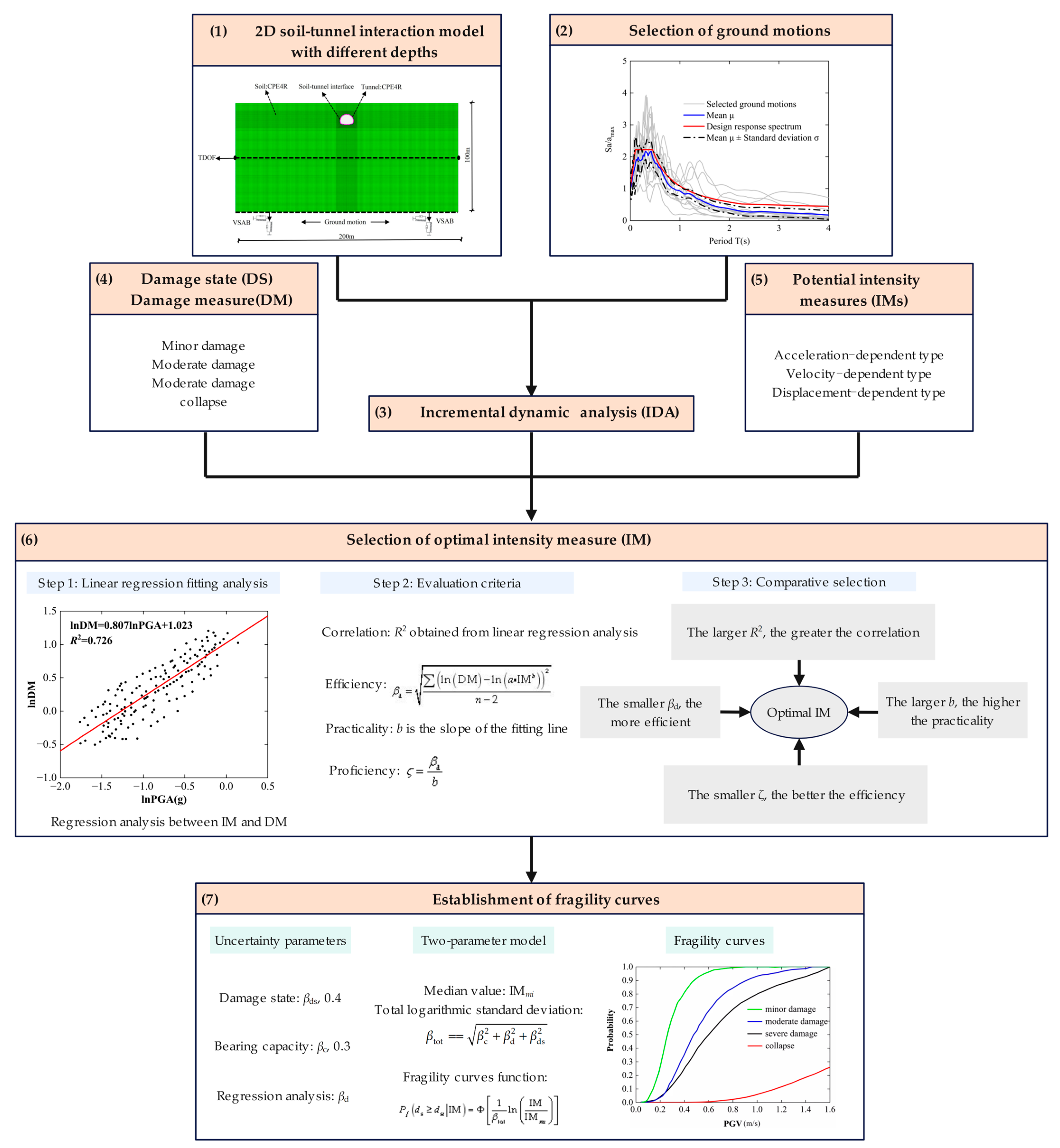
2.2. Main Process of Seismic Fragility Analysis

The proposed process relies on incremental dynamic numerical simulation analysis of the entire process for the horseshoe-shaped tunnel under transverse earthquakes. It can clearly assess the effects of particularities of the ground motion and tunnel burial depth, which are significant parameters affecting the seismic response of tunnels. The procedure for deriving the numerical fragility curve of the tunnel is illustrated in Figure 1. The detailed steps adopted in the proposed methodology are explained as follows:

(1)

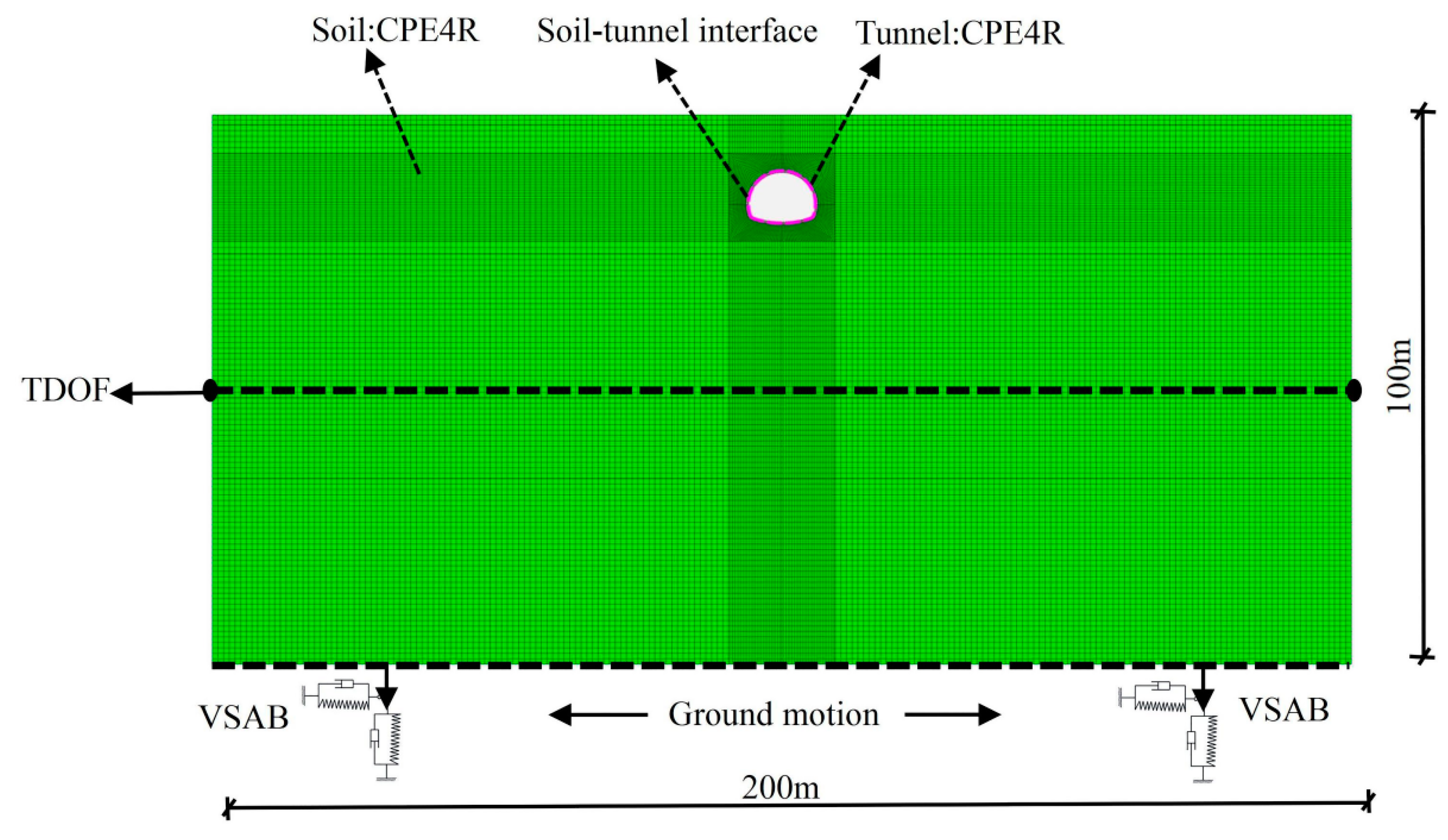
The 2D finite element model of the soil–tunnel interaction system is built.

(2)

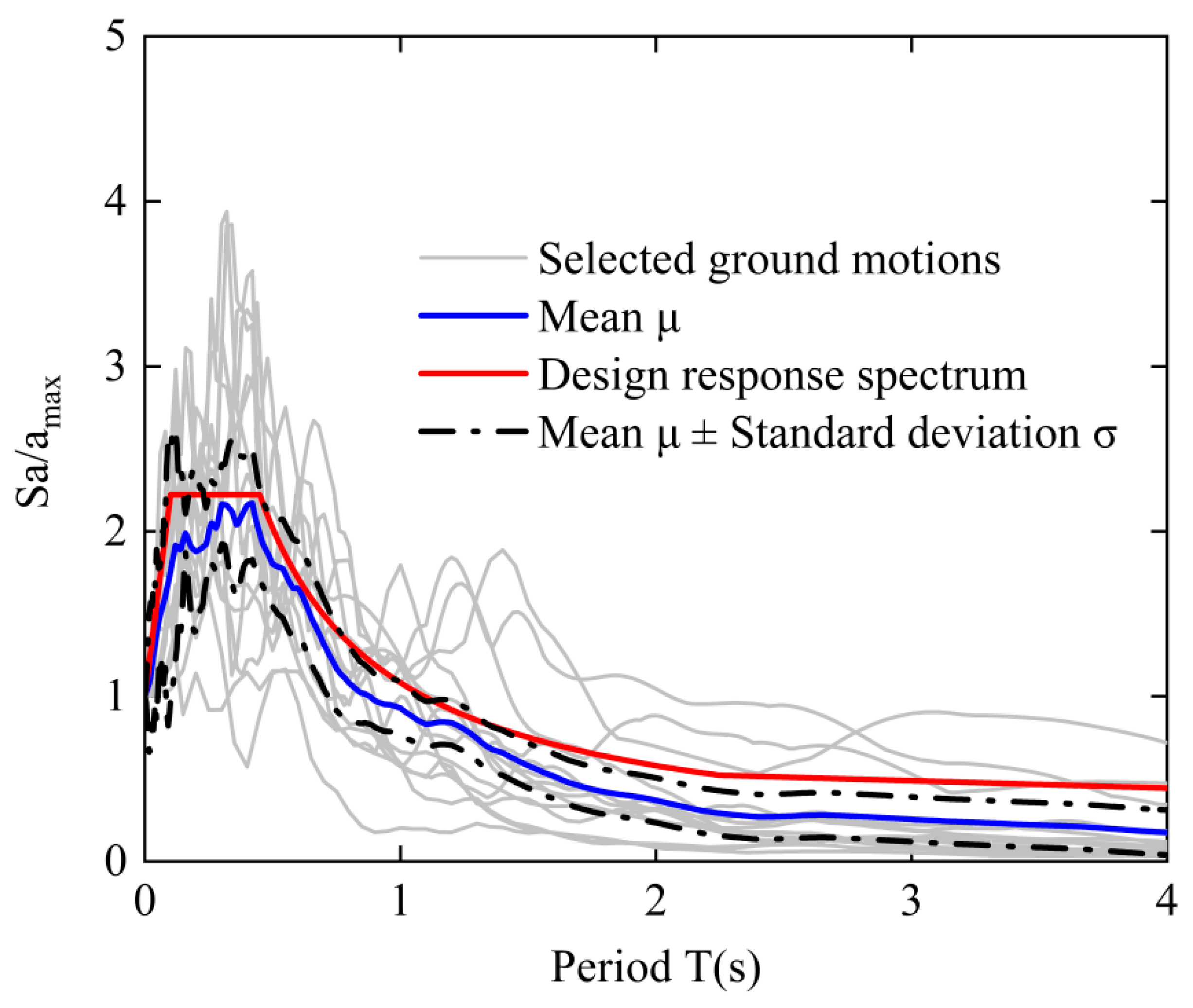
The appropriate ground motions are selected according to the design response spectrum.

(3)

The 2D soil–tunnel numerical models are used to conduct IDA by adjusting PGA, and the evolution of damage with IM is obtained.

(4)

The definition of the damage state (DS) is to quantitatively characterize its DM after being subjected to earthquakes by comparing the actual bending moment M inside the tunnel structure with the design bending moment safety threshold M_RD.

(5)

The commonly used potential IMs are selected.

(6)

The optimal seismic IMs are selected based on the results obtained from IDA and four evaluation criteria.

(7)

Based on DM and the selected optimal IM, the fragility curves are established by using a two-parameter lognormal distribution model.

2.3. Damage States and Damage Measures

The selection of the DM has a significant impact on the fragility analysis, and the definition of DS and the selection of the DM are usually based on the degree of damage. Based on previous research on tunnels considering the normal failure mechanism and the simplicity of indicators, the DM can be described as the ratio between the actual bending moment M and the bearing capacity bending moment M_RD in this study [40,41]. The actual bending moment M through dynamic time history analysis is calculated. The acquisition of bearing capacity bending moment M_RD needs to involve material and geometric properties. The damage states determine the overall macroscopic performance goals, while fragility analysis requires the establishment of damage indicators for each component to more finely describe the degree of local damage. This work defines five damage states: no damage, minor damage, moderate damage, extensive damage, and collapse, as shown in

Table 1. Definition of damage states.

Damage States	Explanation	Range of DM	Median DM
No damage	The tunnel structure and its ancillary facilities are in good condition, without any visible or known physical damage, dysfunction, or performance degradation.	M/MRD ≤ 1.0	-
Minor damage	Slight cracks appear in the tunnel lining or walls but do not hinder traffic.	1.0 < M/MRD ≤ 1.5	1.25
Moderate damage	The tunnel lining or walls appears wider or longer cracks, but the overall function of the tunnel equipment is normal and can operate normally after repair.	1.5 < M/MRD ≤ 2.5	2.00
Extensive damage	The concrete cover of the tunnel spalls off, the rebar is visible, and the concrete lining or walls are deformed.	2.5 < M/MRD ≤ 3.5	3.00
Collapse	The lining or wall of the tunnel breaks, bends, or twists, losing the original shape and support capacity, and the structural function of the tunnel is completely lost.	M/MRD > 3.5	-

.

3. Numerical Modeling

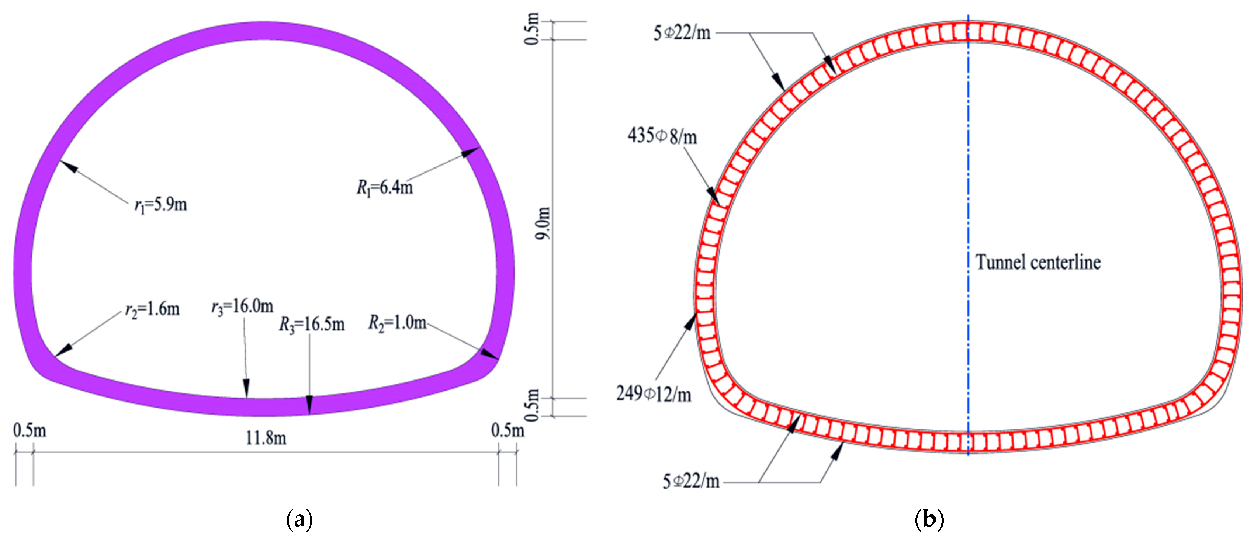
3.1. Description of Horseshoe-Shaped Tunnel

In the current research, the actual double-lane highway horseshoe-shaped tunnel, which serves as a transportation hub, is located in a coastal city in southern China. The size and reinforcement specifications pertaining to the tunnel are depicted in Figure 2. Figure 2a presents the detailed size of the horseshoe-shaped tunnel. The tunnel lining section height is 10.0 m and its width is 12.8 m. In Figure 2a, R and r denote the outer and inner radius of the tunnel lining, respectively. Figure 2b represents the configuration of reinforcement in the horseshoe-shaped tunnel.

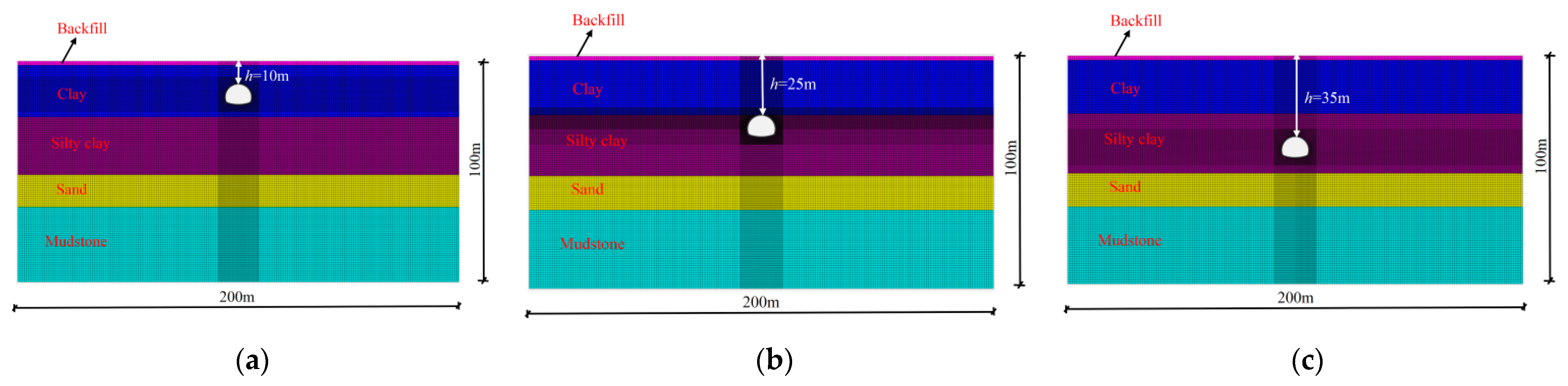
3.2. Numerical Simulation of Geometric Model

The finite element model established in this work mainly includes three parts: the site soil, the tunnel lining, and steel reinforcement. The 2D numerical model of the horseshoe-shaped tunnel considering soil–structure interactions was established by using ABAQUS 2021 software. In the model, the tunnel lining and soil are assigned solid element properties, while the reinforcement bars are embedded as the beam element in the tunnel lining.

The effect of site boundary on the structure can be effectively eliminated by simulating semi-infinite space [50]. In this paper, the width was set as 200 m and the depth was taken as 100 m. To guarantee the precision of the model calculations, the four-node plane strain reduction integral element CPE4R for both soil and tunnel structures was employed, and the maximum mesh size was 1 m. The minimum cell side mesh size of the soil near the tunnel structure and the horseshoe-shaped tunnel was set as 0.2 m. The beam element B21 was used to simulate reinforcement, which can accurately describe the stiffness and strength of reinforcement. The mesh size of the reinforcement was 0.3 m. The schematic diagram of mesh size for the semi symmetric model is shown in Figure 3.

The mesh size was set to be less than 1/10 the seismic wavelength and 1/8 the seismic wavelength, enabling the model to better reflect real behavior and improve the accuracy of numerical simulation. The maximum mesh size l_max can be limited by the following equation [51]:

$$l_{\max }\le \left(\frac{1}{8}~\frac{1}{10}\right)\times \frac{V_{\min }}{f_{\max }}$$

(4)

where V_min is the propagation speed of seismic waves in soil, and f_max is the cutoff frequency of seismic waves. Based on the V_min of the input wave of 471.52 m/s and the f_max of 13 Hz, the maximum grid size was calculated to be 2.77 m. Therefore, the maximum mesh size 1 m can meet the requirements of accurate simulation.

3.3. Boundary and Contact Conditions

The tied degrees of freedom (TDOF) boundary is usually applied to the relative boundary setting of the model, with the aim of ensuring that nodes at the same height can achieve synchronous horizontal displacement under ground motions [52,53]. So as to accurately reflect the realistic situation of the strata, the TDOF boundaries were implemented on the two lateral boundaries so as to more accurately analyze the dynamic response and behavioral characteristics of horseshoe-shaped tunnels in earthquakes. By conducting sensitivity analysis on models of various sizes, it is possible to ensure the free-field conditions of the upper boundary. Meanwhile, the bottom boundary condition was defined as viscous. The TDOF boundary is often imposed to the relative boundary setting, the spring artificial boundary (VSAB). The VSAB was applied to simulate the elastic recovery capacity of a semi-infinite medium, enabling the consideration of radiation damping in dynamic analyses and obtaining accurate dynamic response results. The VSAB can overcome the low-frequency instability problem of viscous boundaries and can simulate the elastic recovery performance of far-field foundations [54]. The parameters of the spring element K and the damping element C for VSAB are described as follows:

$$K_{\mathrm{N}}=2G/r,\hspace{1em}\hspace{1em}{C}_{\mathrm{N}}=\rho C_{\mathrm{P}}$$

(5)

$$K_{\mathrm{T}}=3G/2r,\hspace{1em}\hspace{1em}{C}_{\mathrm{T}}=r{C}_{\mathrm{S}}$$

(6)

where K_N and C_N represent the normal spring stiffness and normal damping coefficient, respectively. K_T and C_T represent the tangential spring stiffness and tangential damping coefficient, respectively. ρ is the density of soil mass. C_P and C_S represent P-wave and S-wave velocities, respectively. And r is the distance, which can be taken as the distance from the center of the near-field structure to the VSAB line or surface.

By utilizing spring and damping elements, the values of spring stiffness and damping coefficient are multiplied by the corresponding boundary nodes’ influence area to establish the VSAB. Figure 4 represents the boundary conditions of the model. When conducting seismic response analysis of structural soil systems, the corresponding ground motion is converted into equivalent nodal forces on artificial boundary nodes. This study employed the analytical method for the static and dynamic coupling effects of the soil–tunnel system, and the entire process was structured into two distinct phases. The initial phase was the static analysis step: the bottom boundary was fixed, and the lateral boundary was constrained to horizontal displacement. In this analysis step, the geostress balance analysis was performed. The second step involved dynamic analysis. The constraint along the lateral boundary was loosened and its vertical displacement was constrained. The equivalent nodal force converted from the acceleration was applied to the bottom boundary.

A primary–secondary contact surface was simulated to describe the dynamic contact characteristics between soil and tunnel lining. Hard contact was applied in the normal direction of the model. When the contact forces produce tension, the contact can be released. The relationship between tangential force and maximum friction force was considered in the model. When the tangential forces exceed the preset friction limit, the tunnel can slide along with the soil. The friction coefficient μ at the interface was determined as 0.6, and the friction angle was taken as 30°. The damping mechanism of materials inside underground structures is able to dissipate energy and reduce the vibration amplitude of the structure, which can significantly alter the dynamic behavior. In structural analysis, the Mohr–Coulomb yield criterion was implemented to explain the soil’s nonlinear response at higher strains.

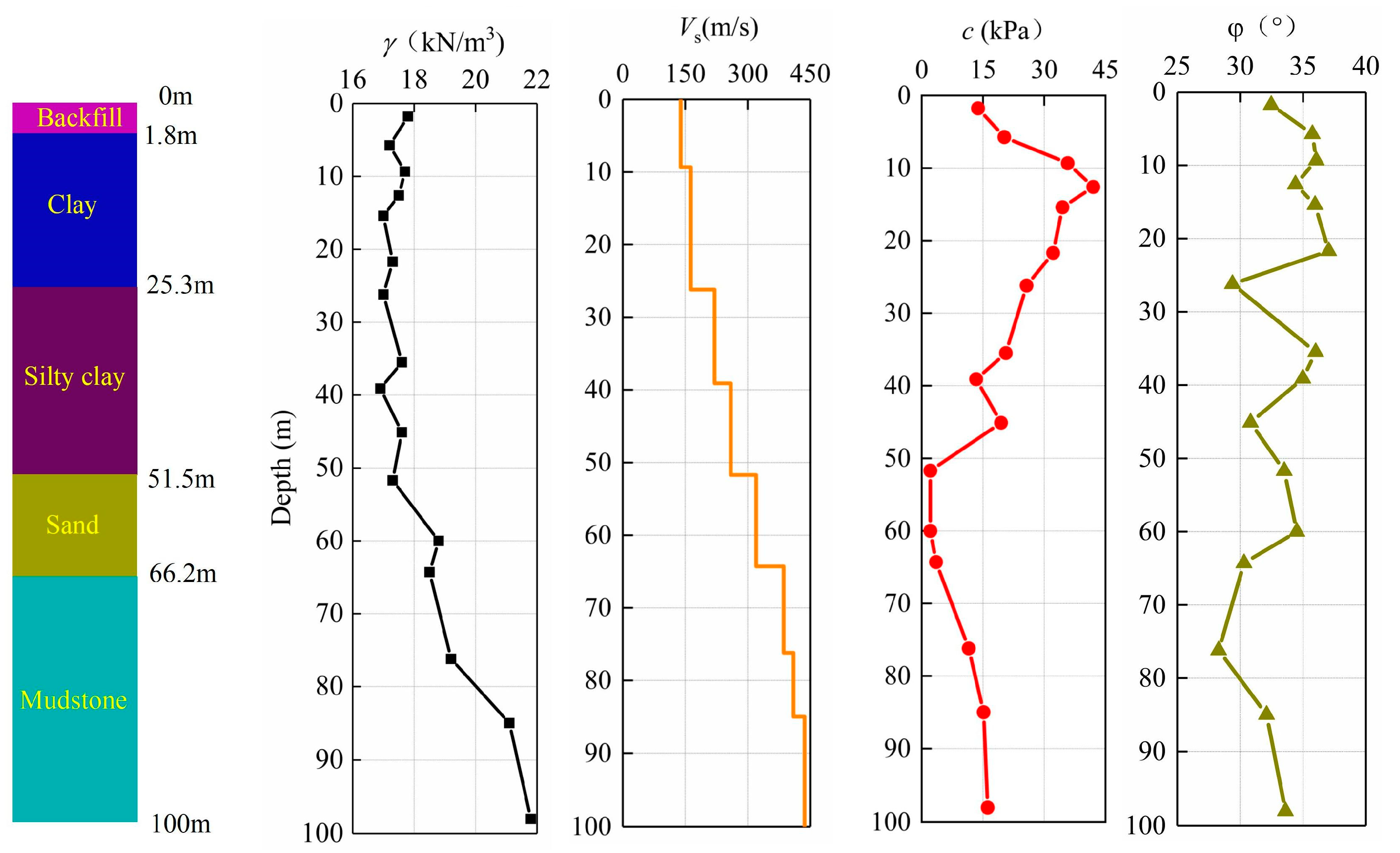
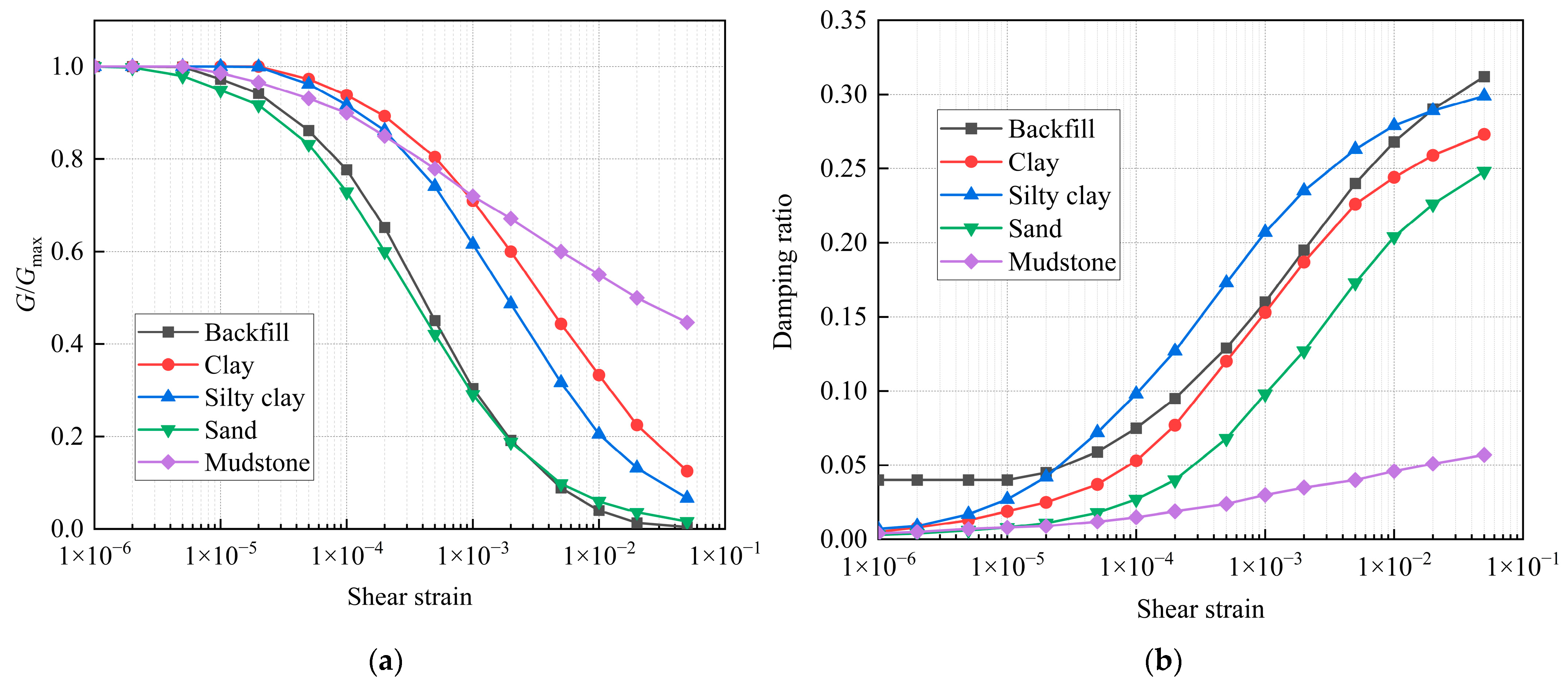
3.4. Material Properties

The viscoelastic plastic model combined with the Mohr–Coulomb yield criterion was used to characterize the nonlinear behavior characteristics exhibited by soil. The soil profile of the selected site was determined as site class III according to the Chinese seismic design code [55]. Figure 5 shows the main soil profiles and physical properties within the region, wherein γ represents the natural unit weight, V_s signifies the shear wave velocities, and c and φ represent the cohesiveness and the internal friction angle, respectively, derived based on the consolidation undrained triaxial shear tests and geological survey data.

When performing dynamic time history analysis, it is imperative to take into account the nonlinearity of the soil stratum and describe the nonlinear behavior of the soil stratum under seismic action through strain compatibility equations. This work adopted the shear strain and damping ratio–shear strain curves of the shear modulus G/G_max as a function of strain level to express nonlinear behavior for the soil stratum, as shown in Figure 6.

The burial depth of soft soil tunnels is usually determined based on factors such as groundwater level, surface load, and underground structure. Therefore, in accordance with the practical requirements of the project, horseshoe-shaped tunnels were established with burial depths of 10 m, 25 m, and 35 m corresponding to shallow burial depth, medium burial depth, and deep burial depth, respectively. The numerical models with different burial depths are shown in Figure 7.

In Figure 8, the material behavior models employed for both concrete and reinforcement within the tunnel construction are presented. The tunnel is reinforced with Q235 steel. The elastic modulus E_s of reinforcement is 200 GPa. And the yield stress f_y is 400 MPa. After the reinforcement reaches the yield stress, it enters the strain-hardening zone, and the hardening coefficient h_d is taken as 0.02. The ultimate strain ε_s of reinforcement is 0.17. The concrete strength of the tunnel lining is C30. The standard value of axial compressive strength f_ck for concrete is 20.1 MPa. In this paper, the plastic damage model was adopted to describe the constitutive behavior of concrete. The constitutive model can explain the change in stiffness attenuation of concrete with tensile and compressive damage under seismic excitations. The concrete material, compression, and tensile damage parameters of C30 are listed in

Table 2. The concrete’s material parameters.

Material	Elastic Modulus Ec (GPa)	Poisson’s Ratio vc	Density ρc (kg/m3)	Dilation Angle ψ (°)	Tensile Yield Stress ft (MPa)	Ultimate Compressive Stress fc (MPa)
C50	30.0	0.2	2450	30.25	2.01	22.83

,

Table 3. Compressive damage parameters d_c.

CompressiveStress(MPa)	15.97	22.83	16.08	13.02	10.80	9.17	7.94	6.24	2.98
Plastic Strain (%)	0	0.070	0.243	0.328	0.411	0.491	0.570	0.725	1.479
dc	0	0.276	0.572	0.656	0.714	0.756	0.788	0.832	0.918

, and

Table 4. Tensile damage parameters d_t.

Tensile Stress (MPa)	2.01	1.74	1.52	1.02	0.36	0.23	0.09	0.06	0.01
Plastic Strain (%)	0	0.009	0.012	0.023	0.096	0.175	0.651	1.279	9.532
dt	0	0.371	0.455	0.647	0.888	0.934	0.978	0.988	0.998

, respectively.

3.5. Selection of Ground Motions

Considering the uncertainty of earthquakes, the selected characteristic parameters of ground motions need to cover a wide range. The magnitude can be determined as 5.0~8.0 Mw, and PGA can be taken as 0.1~1.2 g. Therefore, 15 ground motions were selected from the earthquake database of the Pacific Earthquake Engineering Research Center (PEER). According to the study by Vamvatsikos et al. [56], the 15 seismic ground motions as inputs are sufficient to capture the uncertainties caused by ground motions.

Table 5. The information of the selected ground motions.

NO.	Event	Station	Year	Magnitude (MW)	Epicentral Distance (km)	PGA (g)
Eq.1	Chuetsu-oki, Japan	Tokamachi Chitosecho	2007	6.80	47.73	0.22
Eq.2	Imperial Valley-06	Cerro Prieto	1979	6.53	24.82	0.17
Eq.3	Iwate, Japan	Yuzawa Town	2008	6.90	29.33	0.20
Eq.4	Parkfield-02, CA	Parkfield–Cholame 5W	2004	6.00	13.76	0.23
Eq.5	Chi-Chi, Taiwan	TCU045	1999	7.62	28.95	0.36
Eq.6	Darfield, New Zealand	TPLC	2010	7.00	34.80	0.24
Eq.7	Mammoth Lakes-01	Long Valley Dam	1980	6.06	12.65	0.27
Eq.8	Spitak, Armenia	Gukasian	1988	6.77	36.19	0.15
Eq.9	Hector Mine	Amboy	1999	7.13	47.97	0.18
Eq.10	Kocaeli, Turkey	Yarimca	1999	7.51	5.06	0.35
Eq.11	Northridge-01	Moorpark–Fire Sta	1994	6.69	31.45	0.24
Eq.12	Big Bear-01	Desert Hot Springs	1992	6.46	40.46	0.23
Eq.13	San Fernando	Old Ridge Route	1971	6.61	25.36	0.29
Eq.14	Coalinga-05	Pleasant Valley P.P.–FF	1983	5.77	16.17	0.32
Eq.15	Niigata, Japan	NIG023	2004	6.63	36.47	0.39

briefly lists the information of the selected ground motions.

The selection of ground motions is a critical step in the IDA method. By employing spectrum matching and other methods, the records matching the target response spectrum from representative seismic records were selected. Figure 9 shows the acceleration response spectra of 15 ground motions by comparison with the design response spectrum of site class III based on the Code for Seismic Design of Buildings [55]. To match the design response spectrum, the ratio of the response spectrum acceleration Sa to the maximum seismic acceleration a_max was normalized. In Figure 9, it is evident that the average spectrum of the chosen ground motions aligns well with the standards specified in the China code spectrum. According to the method of IDA, a series of seismic records were selected and gradually amplified from 0.1 g to 1.2 g in a gradient of 0.1 g.

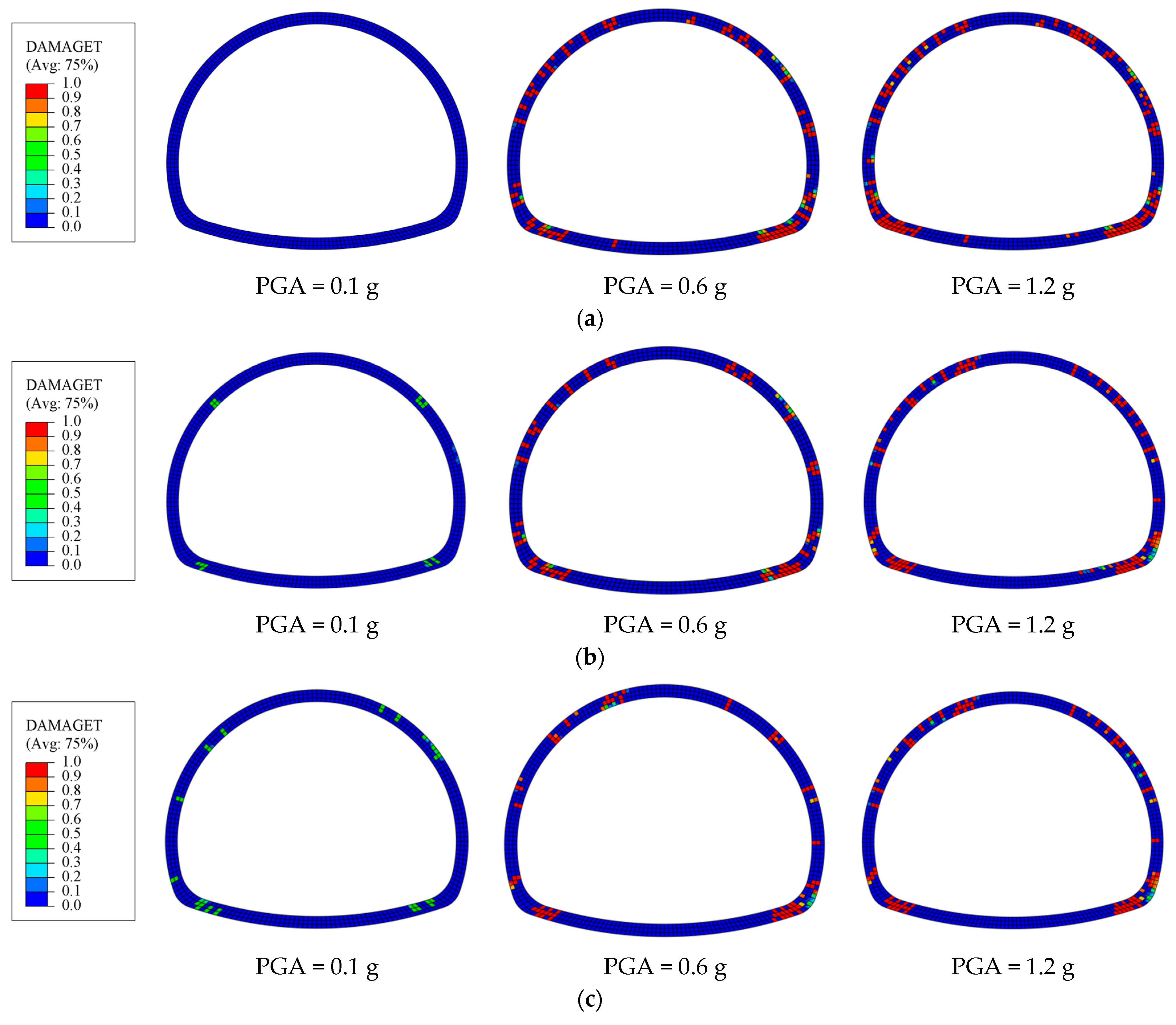
3.6. Structural Damage Evolution Analysis

Figure 10a–c provide representative examples of structural compressive damage distributions for three buried depths under the action of typical ground motion Eq.2, with PGA = 0.1 g, 0.6 g, and 1.2 g, respectively. The factor DAMAGEC represents the degree of compression damage to the lining. When it approaches 1.0, it means that the material has experienced extensive internal damage, almost reaching a state where it cannot continue to effectively bear loads, that is, the tunnel has almost completely lost the compressive capacity in the corresponding area.

As depicted in Figure 10, when PGA = 0.1 g, the tunnels with different burial depths do not show compression damage. And the magnitude of DM calculated based on IDA increases from 0.1 to 0.3 as the burial depth increases. When PGA = 0.6 g, the shallow buried tunnel suffers minor compression damage, while both the medium and deep buried tunnels experience moderate compression damage. Correspondingly, the magnitude of DM increases from 1.1 to 1.8. The analysis result of PGA = 1.2 g is similar to that of PGA = 0.6 g. With an increase in the PGA while maintaining the same burial depth, the compression damage increases slightly, but the impact is not obvious. When the buried depth increases, the connection between the side wall and the bottom plate, called the arch foot, is inclined to be damaged by compression. Therefore, the compressive damage degree of the lining mainly depends on the burial depth of the upper soil.

Figure 11a–c show representative examples of structural tensile damage distributions for three buried depths under the action of typical ground motion Eq.2, with PGA = 0.1 g, 0.6 g, and 1.2 g, respectively. The factor DAMAGET represents the degree of tensile damage to the lining. When it approaches 1.0, the tunnel has almost completely lost the tensile capacity in the corresponding area.

From Figure 11, it can be seen that when PGA = 0.1 g the shallow buried tunnel does not show any tensile damage in elastic state. However, both the medium and deep tunnels show minor tensile damage. Correspondingly, the magnitude of DM based on the IDA calculation results increases from 0.1 to 1.3. As the burial depth increases, the damage first appears at the arch foot and the connection between the top plate and sidewall. Deep buried tunnels have a greater degree of tensile damage than shallow buried tunnels.

When PGA = 0.6 g, extensive tensile damage was observed for the three types of tunnels. It is worth noting that as the depth of burial increases, the magnitude of DM decreases from 2.8 to 2.6. At this time, a large area of extensive tensile damage appears in the concrete in the lining. Complete tensile damage occurs at both the tunnel sidewall and the arch foot. With the gradual increase in burial depth, the zone of damage was observed to shrink. The degree and zone of damage for shallow and medium deep tunnels are similar, and both are more serious than the deep tunnel.

When PGA = 1.2 g, the state of collapse appears in the shallow tunnel. Meanwhile, the value of the DM is increased to 3.7, which can verify the damage state mentioned above. In addition, medium and deep tunnels still exhibit extensive tensile damage. And the DM values calculated based on IDA are 3.4 and 3.1, respectively. The seismic tensile damage range at the connection between the plate and the sidewall is further extended. The damage range and degree of the shallow tunnel are the largest, mainly manifested as significant damage at the connection between the arch and the sidewalls. Compared to the shallow tunnel, the damage of the deep tunnel is significantly reduced.

In summary, the main damage mechanism of the horseshoe-shaped tunnel under earthquake action is not derived from compression damage, but is characterized by tensile damage. The compression damage augments with the increment in burial depth, and mainly depends on the burial depth of the upper soil. If the seismic intensity is small, the tensile damage increases with the burial depth. However, when ground motion intensity increases to a certain level, the tensile damage decreases as the burial depth progressively increases. For the shallow tunnel, tensile damage is most extensive under strong earthquake action. This is mainly because the constraint effect of soil on the tunnel and the propagation of seismic waves vary with different burial depths. Under strong earthquake action, the most easily damaged part of the tunnel lining is the arch foot, followed by the connection between the sidewall and the roof. During seismic design, these parts should be subjected to seismic reinforcement treatment. The results are similar to the observations of Zi et al. [57]. This also substantiates the reliability of the results in the current investigation.

4. Selection of Optimal Intensity Measures

4.1. Potential Intensity Measures

The seismic IM should comprehensively reflect the features of the ground motion experienced by tunnels, including but not limited to the amplitude, frequency composition, and duration. There will be significant differences when using different seismic IMs to evaluate the seismic response. In this study, 17 common IMs were used as the potential IMs and classified into three categories: acceleration-dependent type, velocity-dependent type, and displacement-dependent type.

Table 6. The selected potential IMs.

NO.	Name	Type	Definition
1	Peak ground acceleration	Acceleration-dependent type	$\mathrm{PGA}=\max \left|a\left(t\right)\right|$
2	Arias intensity		$\mathrm{AI}=\frac{\pi }{2g}{\displaystyle {\int }_0^{t_{\max }}{a}^2}\left(t\right)dt$
3	Cumulative absolute velocity		$\mathrm{CAV}={\displaystyle {\int }_0^{t_{\max }}\left|a\left(t\right)\right|}dt$
4	Acceleration root mean square		$a_{\mathrm{rms}}=\sqrt{\frac{1}{t_d}{\displaystyle {\int }_{t_1}^{t_2}{a}^2\left(t\right)dt}}$
5	Characteristic intensity		$I_C=a_{\mathrm{rms}}^{1.5}{t}_d^{0.5}$
6	Acceleration spectrum intensity		$\mathrm{ASI}={\displaystyle {\int }_{0.1}^{0.5}{S}_a}\left(T,\xi \right)dT$
7	Faifar intensity		$I_{\mathrm{F}}=\mathrm{PGV}\cdot t_d^{0.25}$
8	Peak ground velocity	Velocity-dependent type	$\mathrm{PGV}=\max \left|v\left(t\right)\right|$
9	Velocity spectrum intensity		$\mathrm{VSI}={\displaystyle {\int }_{0.1}^{2.5}{S}_v}\left(T,\xi \right)dT$
10	Velocity root mean square		$v_{\mathrm{rms}}=\sqrt{\frac{1}{t_d}{\displaystyle {\int }_{t_1}^{t_2}{v}^2\left(t\right)dt}}$
11	Peak spectrum velocity		$\mathrm{PSV}=\max \left(S_v\left(T,\xi =0.05\right)\right)$
12	Housner velocity intensity		$\mathrm{SI}={\displaystyle {\int }_{0.1}^{2.5}\mathrm{PSV}}\left(T,\xi =0.05\right)dT$
13	Compound velocity		$I_{\mathrm{v}}={\mathrm{PGV}}^{2/3}\cdot t_d^{1/3}$
14	Peak ground displacement	Displacement-dependent type	$\mathrm{PGD}=\max \left|d\left(t\right)\right|$
15	Displacement root mean square		$D_{\mathrm{rms}}=\sqrt{\frac{1}{t_d}{\displaystyle {\int }_{t_1}^{t_2}{d}^2\left(t\right)dt}}$
16	Housner displacement intensity		$P_{\mathrm{d}}=\frac{1}{t_d}{\displaystyle {\int }_{t_1}^{t_2}{d}^2}\left(t\right)dt$
17	Compound displacement		$I_{\mathrm{d}}=\mathrm{PGD}\cdot t_d^{1/3}$

presents the selected potential IMs. In Table 6, t_d denotes the significant duration of ground motion; t_max denotes the total duration of ground motion; v₀ denotes the number of passes through zero in the acceleration time history curve; and t₁ and t₂ represent the time at which the normalized Arias intensity curve reaches 5% and 95% of the total Arias intensity, respectively.

4.2. Correlation Analysis

Correlation analysis is conducted based on the relationship between lnIM and lnDM. The goodness of fit is judged by the correlation coefficient R², which varies from 0 to 1. The larger the R², the smaller the dispersion and the greater the correlation. The optimal IM generally performs as having a larger correlation coefficient, R². Figure 12 shows regression analysis between typical IMs (PGA, PGV, PGD) and corresponding DM for the shallow tunnel. The red dashed line represents IM corresponding to the median value of DM, while the red solid line shows the fitting curve obtained through regression analysis. From Figure 12, it can be observed that the distribution of data points for PGA is the most concentrated, followed by PGV, while the distribution of data points for PGD is the most dispersed. Meanwhile, the R² for PGD was calculated to be the lowest and the fitting effect is the worst. It indicates that compared to PGA and PGV, PGD has the weakest correlation. The larger the R², the more concentrated the result data points obtained from IDA and the greater their correlation. Figure 13 shows the correlation analysis results of 17 potential IMs under different conditions of shallow, medium-deep, and deep tunnels.

As evident from Figure 13a, for shallow tunnel, the association between PGA and DM is the most significant, and the correlation coefficient R² is 0.898, indicating a great linear correlation. The two IMs closely related to DM are a_rms and CAV, and the correlation coefficients R² are 0.762 and 0.761, respectively. On the other hand, it is noteworthy to mention that among the potential IMs, P_d has the weakest correlation with DM, and its correlation coefficient is only 0.266. The second is PGD and I_d, which have low correlation coefficients with DM: only 0.272 and 0.414, respectively.

As shown in Figure 13b, for the medium-deep tunnel, PGV, VSI, and PSV have the greatest correlation with DM, and the correlation coefficients are 0.856, 0.752, and 0.735, respectively. On the contrary, ASI, PGD, and D_rms have the weakest correlation with DM, and the correlation coefficients are 0.575, 0.493, and 0.364, respectively, showing the lowest correlation degree among all IMs.

Figure 13c shows the result of the correlation analysis for the deep tunnel. It can be observed that the correlation coefficient R² between VSI and DM is the largest, reaching 0.839. In addition, two other IMs, PGV and v_rms, are also found to be significantly highly correlated with DM, with correlation coefficients of 0.815 and 0.809, respectively. On the contrary, P_d is the IM with the weakest correlation with DM, and its correlation coefficient is only 0.523. Then, I_d and D_rms have lower correlation coefficients of 0.614 and 0.658, respectively.

As observed in Figure 13a–c, the correlation between the acceleration-dependent-type and velocity-dependent-type IMs and DM is generally larger than the displacement-dependent-type IMs.

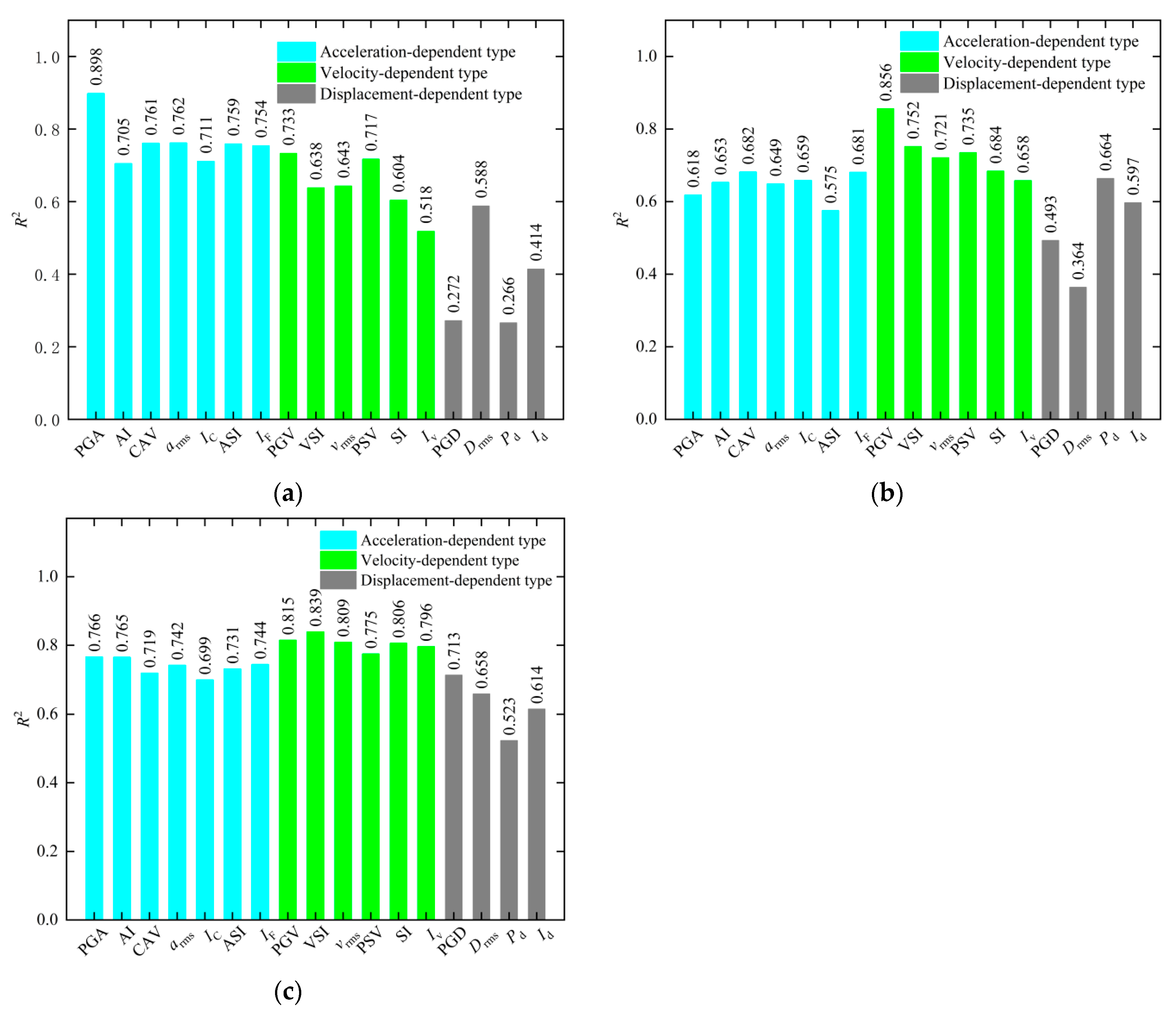
4.3. Efficiency Analysis

The efficiency describes the statistical discrete degree of the structural response measured by DM under the determined IMs. The effective IM is used to select ground motions that can significantly decrease the number of records required for calculation, and obtain the analysis results with the same confidence. The efficiency is evaluated by the logarithmic standard deviation β_d though linear regression. The logarithmic standard deviation β_d can be described as follows:

$${\beta }_{\mathrm{d}}=\sqrt{\frac{{\displaystyle \sum _{i=1}^n{\left[\ln \left(\mathrm{DM}\right)-\left(\ln a+b\ln \left(\mathrm{IM}\right)\right)\right]}^2}}{n-2}}$$

(7)

where n is the number of nonlinear dynamic time history analyses.

The smaller the value of β_d, the lower the discreteness of the incremental dynamic analysis results and the more efficient the selected IM. The results of the efficiency analysis are described in Figure 14.

Based on the data shown in Figure 14a, for the shallow tunnel, it can be seen that PGA, a_rms, and CAV are considered more effective IMs because the logarithmic standard deviation β_d is relatively small. PGA is the most effective IM, and the value of β_d is only 0.203. Followed closely by the other two IMs, the values of β_d are 0.208 and 0.216 respectively. On the contrary, P_d shows the maximum value of β_d, with a value of 0.421, which reveals that P_d has the lowest efficiency. Finally, the logarithmic standard deviation values β_d of D_rms and PGD are 0.403 and 0.386, respectively, lower than P_d.

In Figure 14b, PGV shows the most effectiveness for the medium-deep tunnel, with a logarithmic standard deviation value β_d of only 0.164. It is followed by VSI and PSV; their logarithmic standard deviation values of 0.178 and 0.182, respectively, exhibit a slight elevation compared to PGV. Among the various IMs, D_rms exhibits the lowest efficiency, with a logarithmic standard deviation β_d of 0.451.

As can be seen from Figure 14c, VSI is proved to be the most effective IM based on the fact that its logarithmic standard deviation β_d value is 0.233. And PGV is superior to v_rms; the corresponding β_d values are 0.251 and 0.286, respectively. On the other hand, P_d performs the worst in potential IMs, as it has the highest logarithmic standard deviation β_d value of 0.454. At the same time, D_rms and AI are also less-efficient IMs, as the deviation β_d values are slightly lower than p_d, at 0.422 and 0.388, respectively.

It becomes evident from Figure 14a–c that the logarithmic standard deviation βd values of the acceleration-dependent-type and velocity-dependent-type IMs are larger than those of the displacement-dependent-type IMs. Therefore, acceleration-dependent-type and velocity-dependent-type IMs are more efficient than displacement-dependent-type IMs.

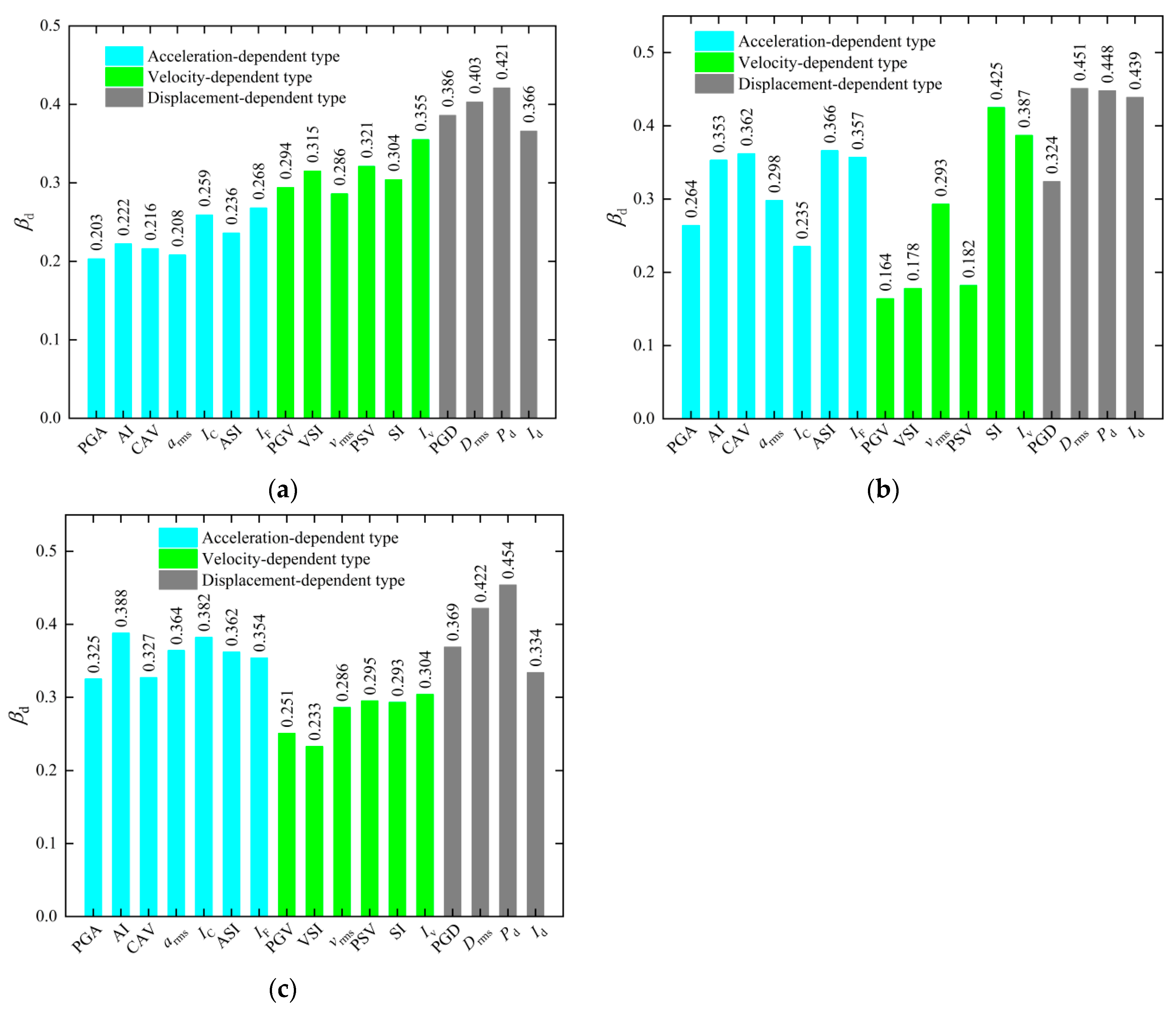
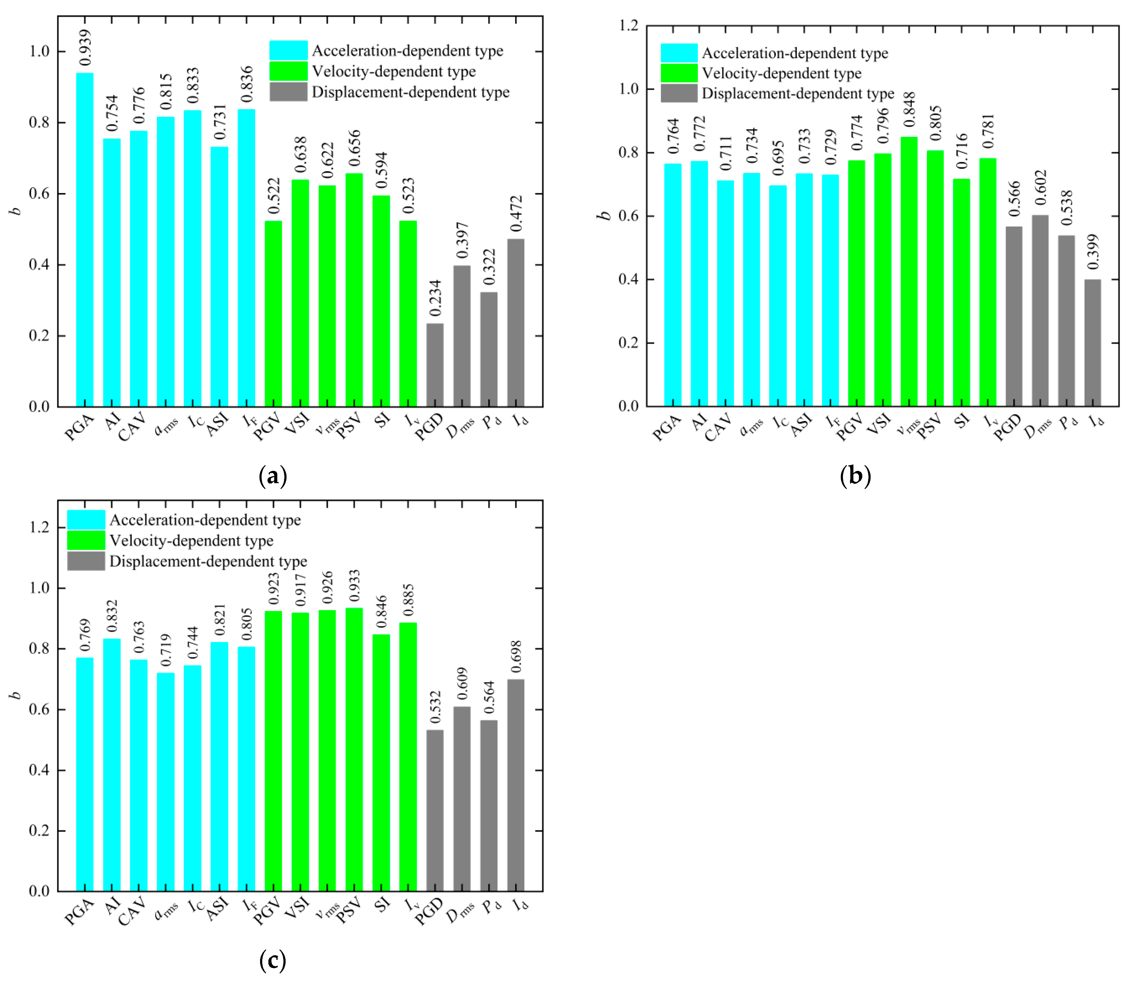
4.4. Practicality Analysis

The practicality of IM refers to the degree to which DM is affected by the change in IM. The practicality is judged according to fitting slope b as the practical coefficient. As the value of b escalates, so does its corresponding level of practicality, indicating that DM is more affected by the change in IM. Figure 15 summarizes the values of the practical coefficient b between IM and DM based on regression analysis for shallow, medium-deep, and deep tunnels.

The comparison in Figure 15a shows that for the shallow tunnel, PGA is considered the most practical IM because the practical coefficient b reaches 0.939. Next, I_F and I_C show sub-optimal practicality, with practical coefficients b of 0.836 and 0.833, respectively, indicating that these two IMs also have higher practicality, but are not as practical as PGA. On the other hand, PGD exhibits the smallest practical coefficient b in this comparison, at just 0.234, indicating that it is the least practical IM. Finally, D_rms and P_d are also proved to be less-practical IMs, with b slightly higher than PGD at 0.397 and 0.322, respectively.

In Figure 15b, v_rms is considered the most practical IM for the medium-deep tunnel. This is followed by PSV and VSI, which are second only to v_rms in terms of practicality. Specifically, the practical coefficients b of the three most practical IMs are 0.848, 0.805, and 0.796, respectively. Relatively speaking, I_d exhibits the lowest practical coefficient b, which means that it has the lowest practicality in the set of IMs. PGD and P_d report the second and third lowest practical coefficient b, respectively. The practical coefficient values of the three least practical IMs are 0.399, 0.538, and 0.566, respectively.

According to the data analysis results shown in Figure 15c, for the deep tunnel, PSV performs best in terms of practicality, with a practical coefficient b of 0.933. Secondly, the practicality of the two IMs, v_rms and PGV, is also outstanding, and the practical coefficients b are 0.926 and 0.923 respectively. In contrast, PGD is the least practical IM of all the comparisons, with a practical coefficient b of only 0.532. Then, P_d and D_rms are the second and third from the bottom, with practical coefficients b of 0.564 and 0.609, respectively.

In Figure 15a–c, it can be seen that the practical coefficient b of the acceleration-dependent-type and velocity-dependent-type IMs is larger than that of the displacement-dependent-type IMs. Therefore, acceleration-dependent-type and velocity-dependent-type IMs are more practical than displacement-dependent-type IMs.

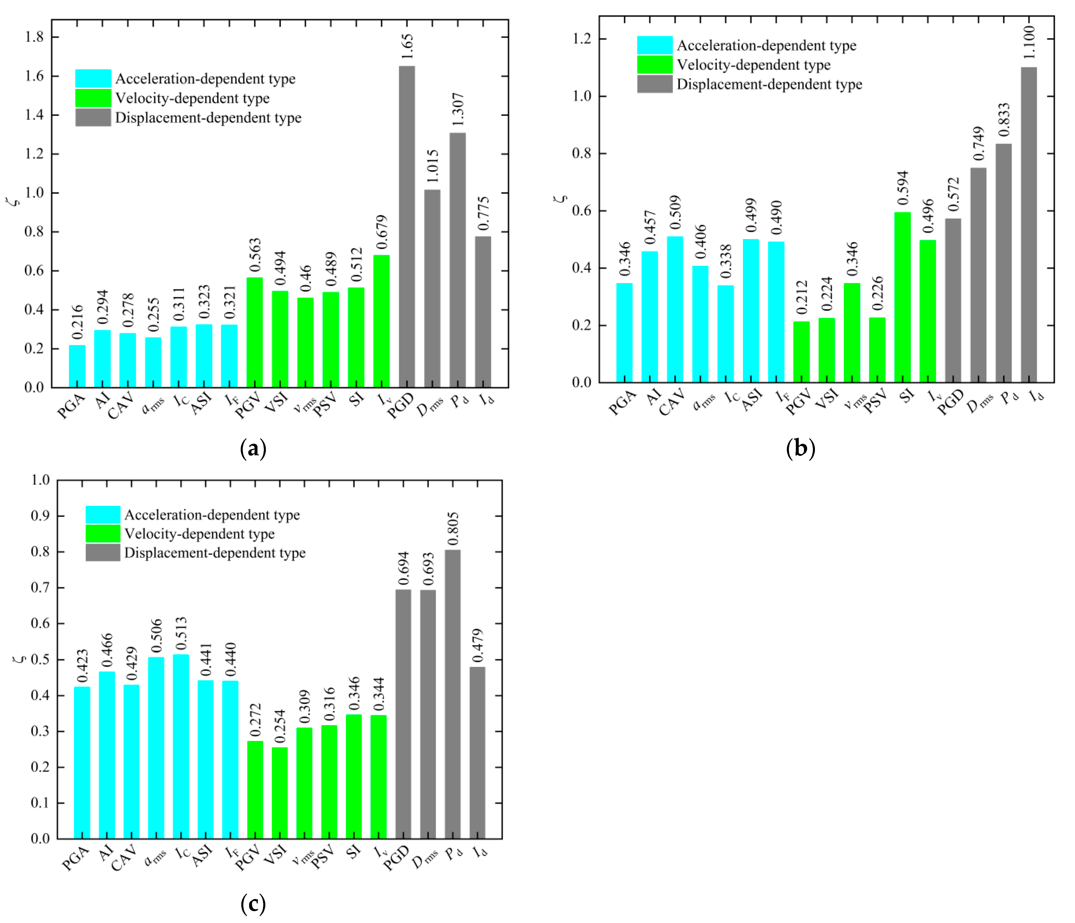
4.5. Proficiency Analysis

There may be some limitations in selecting IMs only depending on the correlation, efficiency, or practicality, which may cause the selected optimal IMs to be unable to reflect the actual situation comprehensively and accurately. Therefore, in order to achieve a more scientific and accurate selection, the proficient coefficient ζ is introduced. The proficient coefficient ζ can be expressed as follows:

$$\zeta =\frac{{\beta }_{\mathrm{d}}}{b}$$

(8)

The smaller the proficient coefficient ζ, the higher the proficiency of the selected IMs. Figure 16 shows the comparative results of the proficient coefficient ζ based on regression analysis for the shallow, medium-deep, and deep tunnels.

As can be seen from Figure 16a, PGA stands as the most efficient IM for the shallow tunnel, because its corresponding proficient coefficient ζ is the lowest, reaching 0.216. Following closely behind a_rms and CAV, the values of the proficient coefficient ζ are close to PGA at 0.255 and 0.278, respectively. However, PGD is considered the least proficient IM because it has the highest value of 1.650. P_d and D_rms are listed after PGD. The values are 1.307 and 1.015, respectively, indicating lower proficiency.

In Figure 16b, for the medium-deep tunnel, PGV stands as the most efficient IM, and the lowest value of the proficient coefficient ζ is 0.212. Meanwhile, VSI and PSV are relatively more highly proficient IMs, and the values are 0.224 and 0.226, respectively. I_d, P_d, and D_rms are relatively less-proficient IMs, and the values of the proficient coefficient ζ are 1.100, 0.833, and 0.749, respectively.

It becomes evident from Figure 16c that for the deep buried tunnel, VSI is the most proficient IM, and the lowest value of the proficient coefficient ζ is 0.254. Next are PGV and v_rms: the the values of the proficient coefficient ζ are 0.272 and 0.309, respectively, indicating lower proficiency compared to VSI. Contrarily, P_d emerges as the least effective IM, exhibiting a proficiency coefficient ζ that reaches a significant value of 0.805. In addition, PGD and D_rms have also been identified as less-proficient Ims; the values of the proficient coefficient ζ are 0.694 and 0.693, respectively.

In Figure 16a–c, it can be seen that the proficient coefficients ζ of the acceleration-dependent-type and velocity-dependent-type IMs are less than that of the displacement-dependent-type IMs. Therefore, the acceleration-dependent-type and velocity-dependent-type IMs are more proficient than the displacement-dependent-type IMs.

4.6. Determining the Optimal IM

To ensure accurate prediction and evaluation of the performance and safety of underground structures such as horseshoe-shaped tunnels under seismic action, it is crucial to determine the optimal IM. Due to the complexity and uncertainty of ground motions, selecting the IM that can effectively transmit the basic dynamic characteristics is important. Although previous studies have extensively focused on determining the optimal IM for aboveground buildings, such optimization research in underground structures, especially in tunnel engineering, is still rare. Therefore, based on the above analysis, the three most correlated, efficient, practical, and proficient IMs are used to select the optimal IM suitable for the shallow, medium-deep, and deep tunnels, as shown in Figure 17.

From Figure 17a, it is evident that for shallow tunnels, PGA is the optimal IM, closely followed by a_rms and CAV in descending order of optimality. In Figure 17b, for medium deep tunnel, PGV is the optimal IM. Following closely are VSI and PSV. According to the data analysis results shown in Figure 17c, under the condition of deep tunnel, the optimal IM is VSI, followed by PGV and v_rms. And for medium deep tunnel and deep tunnel, velocity-dependent-type IMs have more advantages. Finally, in the conventional seismic design and response analysis of tunnels, displacement-dependent-type IMs are not the best considerations. Therefore, the burial depth has a significant influence on the selection of IMs in fragility analysis.

5. Establishment of Fragility Curves

By substituting the median values of damage states into the regression analysis results and using the selected optimal IM, the fragility curves can be established for tunnels with different burial depths.

Table 7. The values of IM_mi for horseshoe-shaped tunnels with different burial depths.

Tunnel Type	IM (Unit)	Minor Damage	Moderate Damage	Extensive Damage
Shallow tunnel	PGA (g)	0.516	1.184	1.433
Medium-deep tunnel	PGV (m/s)	0.601	1.217	1.925
Deep tunnel	VSI (m)	0.948	1.785	2.616

presents the IM_mi corresponding to the median values of three damage states for horseshoe-shaped tunnels in soft soil. According to Equation (3), the total logarithmic standard deviation β_tot is obtained. The values of β_tot are calculated as 0.539, 0.526, and 0.552, respectively. By substituting the obtained β_tot and IM_mi into Equation (2), the fragility curves are obtained. Figure 18 shows the fragility curves corresponding to different damage states.

The fragility curves derived from this study are valuable for application in seismic risk assessment. By utilizing the fragility curves, it is possible to accurately predict the probability of minor, moderate, and even extensive damage to horseshoe-shaped tunnels under different seismic intensities, providing scientific basis for the seismic design of tunnels, safety assessment, and post-earthquake repair strategies. As depicted in Figure 18, with the continuous increase in seismic intensity, the probability of the structure experiencing various damage states gradually increases close to 100%. Given identical seismic intensities, the likelihood of extensive damage is the lowest, followed by moderate damage, and the probability of minor damage is the highest.

6. Conclusions

In this paper, distinct finite element analysis models have been developed to investigate the dynamic soil–tunnel interaction, encompassing burial depths of 10 m, 25 m, and 35 m, representing shallow tunnel, medium-deep tunnel and deep tunnel configurations, and the impact of burial depth on seismic tensile and compressive damage has been rigorously analyzed through the application of the IDA methodology. Drawing upon the four criteria of correlation, efficiency, practicality, and proficiency, 17 potential IMs were evaluated comprehensively to obtain the optimal IMs for horseshoe-shaped tunnels with different burial depths in soft soil. The seismic fragility curves of the horseshoe-shaped tunnels were established by adopting the optimal IMs. The following conclusions could be drawn:

(1)

The seismic damage of horseshoe-shaped tunnels is mainly tensile damage, while the compression damage is not obvious. The extent of compression damage sustained by the tunnel intensifies as the burial depth increases, primarily being influenced by the depth of the overlying soil. As the burial depth increases, the tensile damage of the tunnel initially exhibits an upward trend, subsequently followed by a decrease during the earthquake process.

(2)

In the case of shallow tunnels, the optimal IM is PGA, with arms and CAV occupying subsequent positions. For the medium-deep tunnel, PGV is the optimal IM. Following closely are VSI and PSV. And under the conditions of the deep tunnel, the optimal IM is VSI, followed by PGV and v_rms.

(3)

The acceleration-dependent-type IMs are particularly adept at forecasting the seismic response of the shallow tunnel, while for the medium-deep tunnel and deep tunnel, velocity-dependent-type IMs have more advantages in predicting the seismic response.

(4)

At a constant seismic intensity, the likelihood of extensive damage is the lowest, followed by moderate damage, and the likelihood of minor damage is the highest. The fragility curves derived from our study provide valuable insights for evaluating the seismic risk associated with horseshoe-shaped tunnels constructed in soft soil.

(5)

The findings can be used in future studies as a basis for fragility analysis of tunnels affected by burial depth conditions. Future research can consider additional geological factors, especially the presence of clay layers at the underside of the tunnels, toward more comprehensive probabilistic seismic fragility analysis.

References

1. He, H.; Wang, S.; Shen, W.; Zhang, W. The influence of pipe-jacking tunneling on deformation of existing tunnels in soft soils and the effectiveness of protection measures. Transp. Geotech. 2023, 42, 101061. [Google Scholar] [CrossRef]
2. Jin, H.; Yuan, D.; Jin, D.; Wu, J.; Wang, X.; Han, B.; Mao, J. Ground deformation induced by shield tunneling posture in soft soil. Tunn. Undergr. Space Technol. 2023, 139, 105227. [Google Scholar] [CrossRef]
3. Mohsenian, V.; Hajirasouliha, I.; Mariani, S.; Nikkhoo, A. Seismic reliability assessment of RC tunnel-form structures with geometric irregularities using a combined system approach. Soil Dyn. Earthq. Eng. 2020, 139, 106356. [Google Scholar] [CrossRef]
4. Feng, S.; Lei, H.A. Settlement prediction model considering tidal loading and traffic loading of soft soil subgrade. Comput. Geotech. 2022, 144, 104639. [Google Scholar] [CrossRef]
5. Lei, H.; Li, B.; Lu, H.; Ren, Q. Dynamic deformation behavior and cyclic degradation of ultrasoft soil under cyclic loading. J. Mater. Civ. Eng. 2016, 28, 04016135. [Google Scholar] [CrossRef]
6. Sun, Q.; Dias, D.; e Sousa, L.R. Soft soil layer-tunnel interaction under seismic loading. Tunn. Undergr. Space Technol. 2020, 98, 103329. [Google Scholar] [CrossRef]
7. Hao, Y.H.; Azzam, R. The plastic zones and displacements around underground openings in rock masses containing a fault. Tunn. Undergr. Space Technol. 2005, 20, 49–61. [Google Scholar] [CrossRef]
8. Azadiab, M. The seismic behavior of urban tunnels in soft saturated soils. Procedia Eng. 2011, 14, 3069–3075. [Google Scholar] [CrossRef]
9. Iida, H.; Hiroto, T.; Yoshida, N.; Iwafuji, M. Damage to Daikai subway station. Soils Found. 1996, 36, 283–300. [Google Scholar] [CrossRef]
10. Lu, C.C.; Hwang, J.H. Damage analysis of the new Sanyi railway tunnel in the 1999 Chi-Chi earthquake: Necessity of second lining reinforcement. Tunn. Undergr. Space Technol. 2018, 73, 48–59. [Google Scholar] [CrossRef]
11. Wang, Z.Z.; Zhang, Z. Seismic damage classification and risk assessment of mountain tunnels with a validation for the 2008 Wenchuan earthquake. Soil Dyn. Earthq. Eng. 2013, 45, 45–55. [Google Scholar] [CrossRef]
12. Shen, Y.; Gao, B.; Yang, X.; Tao, S. Seismic damage mechanism and dynamic deformation characteristic analysis of mountain tunnel after Wenchuan earthquake. Eng. Geol. 2014, 180, 85–98. [Google Scholar] [CrossRef]
13. Tothong, P.; Luco, N. Probabilistic seismic demand analysis using advanced ground motion intensity measures. Earthq. Eng. Struct. Dyn. 2007, 36, 1837–1860. [Google Scholar] [CrossRef]
14. Giovenale, P.; Cornell, C.A.; Esteva, L. Comparing the adequacy of alternative ground motion intensity measures for the estimation of structural responses. Earthq. Eng. Struct. Dyn. 2004, 33, 951–979. [Google Scholar] [CrossRef]
15. Jiang, J.W.; Xu, C.S.; Du, X.L.; Chen, G.X.; Xu, Z.G. Optimal Index of Earthquake Intensity Measures for Seismic Design of Underground Frame Structure of Shallow-Buried Subway Station. Chin. J. Geotech. Eng. 2023, 45, 318–326. (In Chinese) [Google Scholar]
16. De Biasio, M.; Grange, S.; Dufour, F.; Allain, F.; Petre-Lazar, I. Intensity measures for probabilistic assessment of non-structural components acceleration demand. Earthq. Eng. Struct. Dyn. 2015, 44, 2261–2280. [Google Scholar] [CrossRef]
17. Finn, W.D.L. State-of-the-art of geotechnical earthquake engineering practice. Soil Dyn. Earthq. Eng. 2000, 20, 1–15. [Google Scholar] [CrossRef]
18. Hao, M.; Xie, L.; Li, W. Study on physical measure of seismic intensity based on damage to masonry structures. Earthq. Eng. Eng. Vib. 2007, 27, 27. [Google Scholar]
19. Shome, N.; Cornell, C.A.; Bazzurro, P.; Carballo, J.E. Earthquakes, records, and nonlinear responses. Earthq. Spectra 1998, 14, 469–500. [Google Scholar] [CrossRef]
20. Dong, Z.F.; Cao, X.W.; Zeng, F.K.; Zhu, H.Y.; Liu, G.Z. Research on Reasonable Ground Motion Intensity Measure in Lateral Seismic of Tunnel. J. Basic Sci. Eng. 2022, 30, 776–789. (In Chinese) [Google Scholar]
21. Lin, L.; Naumoski, N.; Saatcioglu, M.; Foo, S. Improved intensity measures for probabilistic seismic demand analysis. Part 1: Development of improved intensity measures. Can. J. Civ. Eng. 2011, 38, 79–88. [Google Scholar] [CrossRef]
22. Zhang, C.M.; Zhong, Z.L.; Zhen, L.B.; Shen, Y.Y.; Zhao, M. Seismic intensity measures for the damage evaluation of circular tunnels. Eng. Mech. 2021, 38, 100–108. (In Chinese) [Google Scholar]
23. Luco, N.; Cornell, C.A. Structure-specific scalar intensity measures for near-source and ordinary earthquake ground motions. Earthq. Spectra 2007, 23, 357–392. [Google Scholar] [CrossRef]
24. Mackie, K.; Stojadinović, B. Probabilistic seismic demand model for California highway bridges. J. Bridge Eng. 2001, 6, 468–481. [Google Scholar] [CrossRef]
25. Khosravikia, F.; Clayton, P. Updated evaluation metrics for optimal intensity measure selection in probabilistic seismic demand models. Eng. Struct. 2020, 202, 109899. [Google Scholar] [CrossRef]
26. Heshmati, M.; Jahangiri, V. Appropriate intensity measures for probabilistic seismic demand estimation of steel diagrid systems. Eng. Struct. 2021, 249, 113260. [Google Scholar] [CrossRef]
27. Nguyen, D.D.; Park, D.; Shamsher, S.; Nguyen, V.Q.; Lee, T.H. Seismic vulnerability assessment of rectangular cut-and-cover subway tunnels. Tunn. Undergr. Space Technol. 2019, 86, 247–261. [Google Scholar] [CrossRef]
28. Chen, Z.; Wei, J. Correlation between ground motion parameters and lining damage indices for mountain tunnels. Nat. Hazards 2013, 65, 1683–1702. [Google Scholar] [CrossRef]
29. Sun, B.; Zhang, G.; Xue, B.; Kou, L.; Hu, L.; Liu, W. The analysis of the optimal scalar and vector intensity measurements for seismic performance assessment of deep-buried hydraulic arched tunnels. Undergr. Space 2023, 9, 218–233. [Google Scholar] [CrossRef]
30. Sun, B.; Deng, M.; Zhang, S.; Wang, C.; Li, Y.; Song, R. Application of the endurance time methodology on seismic analysis and performance assessment of hydraulic arched tunnels. Tunn. Undergr. Space Technol. 2021, 115, 104022. [Google Scholar] [CrossRef]
31. Huang, Z.K.; Argyroudis, S.; Pitilakis, K.; Zhang, D.M.; Tsinidis, G. Fragility assessment of tunnels in soft soils using artificial neural networks. Undergr. Space 2022, 7, 242–253. [Google Scholar] [CrossRef]
32. Huang, Z.K.; Pitilakis, K.; Argyroudis, S.; Tsinidis, G.; Zhang, D.M. Selection of optimal intensity measures for fragility assessment of circular tunnels in soft soil deposits. Soil Dyn. Earthq. Eng. 2021, 145, 106724. [Google Scholar] [CrossRef]
33. Zhong, Z.; Shen, Y.; Zhao, M.; Li, L.Y.; Du, X. Seismic performance evaluation of two-story and three-span subway station in different engineering sites. J. Earthq. Eng. 2022, 26, 7505–7535. [Google Scholar] [CrossRef]
34. Zhuang, H.; Yang, J.; Chen, S.; Dong, Z.; Chen, G. Statistical numerical method for determining seismic performance and fragility of shallow-buried underground structure. Tunn. Undergr. Space Technol. 2021, 116, 104090. [Google Scholar] [CrossRef]
35. Xu, Z.; Zhuang, H.; Xia, Z.; Yang, J.; Bu, X. Study on the effect of burial depth on seismic response and seismic intensity measure of underground structures. Soil Dyn. Earthq. Eng. 2023, 166, 107782. [Google Scholar] [CrossRef]
36. Cilingir, U.; Madabhushi, S.P.G. Effect of depth on seismic response of circular tunnels. Can. Geoech. J. 2011, 48, 117–127. [Google Scholar] [CrossRef]
37. Hu, X.; Zhou, Z.; Chen, H.; Ren, Y. Seismic fragility analysis of tunnels with different buried depths in a soft soil. Sustainability 2020, 12, 892. [Google Scholar] [CrossRef]
38. Chian, S.C.; Madabhushi, S.P.G. Effect of buried depth and diameter on uplift of underground structures in liquefied soils. Soil Dyn. Earthq. Eng. 2012, 41, 181–190. [Google Scholar] [CrossRef]
39. Cilingir, U.; Madabhushi, S.G. Effect of depth on the seismic response of square tunnels. Soils Found. 2011, 51, 449–457. [Google Scholar] [CrossRef]
40. Argyroudis, S.A.; Pitilakis, K.D. Seismic fragility curves of shallow tunnels in alluvial deposits. Soil Dyn. Earthq. Eng. 2012, 35, 1–12. [Google Scholar] [CrossRef]
41. Tsinidis, G.; de Silva, F.; Anastasopoulos, I.; Bilotta, E.; Bobet, A.; Hashash, Y.M.; Fuentes, R. Seismic behaviour of tunnels: From experiments to analysis. Tunn. Undergr. Space Technol. 2020, 99, 103334. [Google Scholar] [CrossRef]
42. Jiang, J.; Tao, R.; El Naggar, M.H.; Liu, H.; Du, X. Seismic performance and vulnerability analysis for bifurcated tunnels in soft soil. Comput. Geotech. 2024, 167, 106065. [Google Scholar] [CrossRef]
43. Miao, Y.; Zhong, Y.; Ruan, B.; Cheng, K.; Wang, G. Seismic response of a subway station in soft soil considering the structure-soil-structure interaction. Tunn. Undergr. Space Technol. 2020, 106, 103629. [Google Scholar] [CrossRef]
44. Pham, V.V.; Do, N.A.; Dias, D. Sub-rectangular tunnel behavior under seismic loading. Appl. Sci. 2021, 11, 9909. [Google Scholar] [CrossRef]
45. Huang, Z.K.; Pitilakis, K.; Tsinidis, G.; Argyroudis, S.; Zhang, D.M. Seismic vulnerability of circular tunnels in soft soil deposits: The case of Shanghai metropolitan system. Tunn. Undergr. Space Technol. 2020, 98, 103341. [Google Scholar] [CrossRef]
46. Zhong, Z.; Feng, L.; Shen, J.; Du, X. Seismic fragility analysis of subway station structure subjected to sequence-type ground motions. Tunn. Undergr. Space Technol. 2024, 144, 105570. [Google Scholar] [CrossRef]
47. Xu, M.; Cui, C.; Zhao, J.; Xu, C.; Zhang, P.; Su, J. Fuzzy seismic fragility analysis of underground structures considering multiple failure criteria. Tunn. Undergr. Space Technol. 2024, 145, 105614. [Google Scholar] [CrossRef]
48. Huang, Z.; Cheng, Y.; Zhang, D.; Yan, D.; Shen, Y. Seismic fragility and resilience assessment of shallowly buried large-section underground civil defense structure in soft soils: Framework and application. Tunn. Undergr. Space Technol. 2024, 146, 105640. [Google Scholar] [CrossRef]
49. Stefanidou, S.P.; Kappos, A.J. Methodology for the development of bridge-specific fragility curves. Earthq. Eng. Struct. Dyn. 2017, 46, 73–93. [Google Scholar] [CrossRef]
50. Du, X.L.; Zhao, M. Stability and identification for rational approximation of frequency response function of unbounded soil. Earthq. Eng. Struct. Dyn. 2010, 39, 165–186. [Google Scholar] [CrossRef]
51. Kuhlemeyer, R.L.; Lysmer, J. Finite element method accuracy for wave propagation problems. J. Soil. Mech. Found. Div. 1973, 99, 421–427. [Google Scholar] [CrossRef]
52. Tsinidis, G.; Pitilakis, K.; Madabhushi, G.; Heron, C. Dynamic response of flexible square tunnels: Centrifuge testing and validation of existing design methodologies. Geotechnique 2015, 65, 401–417. [Google Scholar] [CrossRef]
53. Li, Y.; Zhao, M.; Xu, C.S.; Du, X.L.; Li, Z. Earthquake input for finite element analysis of soil-structure interaction on rigid bedrock. Tunn. Undergr. Space Technol. 2018, 79, 250–262. [Google Scholar] [CrossRef]
54. Li, Z.Y.; Hu, Z.Q.; Lin, G.; Li, J.B. A scaled boundary finite element method procedure for arch dam-water-foundation rock interaction in complex layered half-space. Comput. Geotech. 2022, 141, 104524. [Google Scholar] [CrossRef]
55. Ministry of Housing and Urban-Rural Development. Code for Seismic Design of Buildings; China Architecture and Building Press: Beijing, China, 2001. (In Chinese) [Google Scholar]
56. Vamvatsikos, D.; Cornell, C.A. Incremental dynamic analysis. Earthq. Eng. Struct. Dyn. 2002, 31, 491–514. [Google Scholar] [CrossRef]
57. Zi, H.; Ding, Z.; Ji, X.; Liu, Z.; Shi, C. Effect of voids on the seismic vulnerability of mountain tunnels. Soil Dyn. Earthq. Eng. 2021, 148, 106833. [Google Scholar] [CrossRef]
Figure 1. Procedure diagram for the establishment of fragility curves of horseshoe-shaped tunnels.
Symmetry 16 00859 g001
Figure 2. Schematic diagram of horseshoe-shaped tunnel: (a) cross-section size; (b) reinforcement arrangement.
Symmetry 16 00859 g002
Figure 3. Schematic diagram mesh size for the semi symmetric model.
Symmetry 16 00859 g003
Figure 4. The boundary conditions of the model.
Symmetry 16 00859 g004
Figure 5. Soil profile and geotechnical properties with depth.
Symmetry 16 00859 g005
Figure 6. Adopted shear modulus reduction curves and damping curves for soil stratum: (a) G–shear strain curves of soil stratum; (b) damping ratio–shear strain curves of soil stratum.
Symmetry 16 00859 g006
Figure 7. Finite element model of soil–tunnel system with different burial depths: (a) shallow burial depth; (b) medium depth; (c) deep burial depth.
Symmetry 16 00859 g007
Figure 8. The constitutive models of the materials used in tunnel lining: (a) reinforcement; (b) concrete.
Symmetry 16 00859 g008
Figure 9. The response spectrum curve of the selected ground motions and the design response spectrum curves.
Symmetry 16 00859 g009
Figure 10. The compression damage distributions under action of typical ground motion Eq.2: (a) shallow tunnel; (b) medium-deep tunnel; (c) deep tunnel.
Symmetry 16 00859 g010
Figure 11. The tensile damage distributions under action of typical ground motion Eq.2: (a) shallow tunnel; (b) medium-deep tunnel; (c) deep tunnel.
Symmetry 16 00859 g011
Figure 12. Linear regression analysis between typical IMs and DM for the shallow tunnel: (a) PGA, R2 = 0.898; (b) PGV, R2 = 0.733; (c) PGD, R2 = 0.272.
Symmetry 16 00859 g012
Figure 13. Correlation coefficient R2 for the 17 potential IMs based on the regression analysis of the tunnel: (a) shallow tunnel; (b) medium-deep tunnel; (c) deep tunnel.
Symmetry 16 00859 g013
Figure 14. Efficiency parameter βd for the 17 potential IMs based on the nonlinear dynamic analysis of the tunnel: (a) shallow tunnel; (b) medium-deep tunnel; (c) deep tunnel.
Symmetry 16 00859 g014
Figure 15. Practical coefficient b for the 17 potential IMs based on the regression analysis of the tunnel: (a) shallow tunnel; (b) medium-deep tunnel; (c) deep tunnel.
Symmetry 16 00859 g015
Figure 16. Proficient coefficient ζ for the 17 potential IMs based on the regression analysis of the tunnel: (a) shallow tunnel; (b) medium deep tunnel; (c) deep tunnel.
Symmetry 16 00859 g016
Figure 17. Three most correlated, efficient, practical, and proficient IMs for tunnels: (a) shallow tunnel; (b) medium-deep tunnel; (c) deep tunnel.
Symmetry 16 00859 g017
Figure 18. The fragility curves for the horseshoe-shaped tunnel in soft soil: (a) shallow tunnel; (b) medium-deep tunnel; (c) deep tunnel.
Symmetry 16 00859 g018