Article

Analyzing the Approximate Error and Applicable Condition of the Fractional Reduced Differential Transform Method

1
School Automation & Electrical Engineering, Zhejiang University Science & Technology, Hangzhou 310023, China
2
Zhejiang Provincial Industrial Institute of Robotics, Hangzhou 310023, China
3
State Industrial Institute of Robotics, Hangzhou 310023, China
Symmetry 2024, 16(7), 912; https://doi.org/10.3390/sym16070912
Submission received: 16 May 2024 / Revised: 2 July 2024 / Accepted: 6 July 2024 / Published: 17 July 2024
(This article belongs to the Section Mathematics)

Abstract

:
The fractional reduced differential transform method is a finite iterative method based on infinite fractional expansions. The obtained result is the approximation of the real value. Currently, there are few reports on the approximate error and applicable condition. In this paper, we study the factors related to the approximate errors according to the fractional expansions. Our research shows that the approximate errors relate not only to fractional order but also to time t, and that they increase rapidly with time t. This method can only be applied within a certain time range, and the time range is relevant to fractional order and fractional expansions. We can ascertain this time range according to the absolute error and the relative error. Many obtained achievements may be incorrect if the applicable conditions are not satisfied. Some examples presented in this paper verify our analysis.

1. Introduction

Fractional calculus is an extension of integer calculus from the integer dimension to the fractional dimension, and can be applied to depict real physical systems with arbitrary accuracy. Treatments of fractional models appear in many areas, including signal processing [1], image processing, control engineering [2], mechanical engineering, and more [3,4,5].
The symmetry design of the system includes integer calculus and fractional calculus. Fractional calculus can be applied for modeling many problems in real-life situations. The fractional calculus is defined by a convolution operation, and is computationally complex. Simplifying this computation is an important research topic in the field of fractional calculus. Many approximate approaches have been proposed for this issue [6,7,8,9,10,11]. Without exception, any approximate method can obtain only approximate solutions, never exact solutions. Thus, there must exist an approximate error between the approximate solution and the exact solution. Only within the allowable range of the approximate error can this approximate method be correct, otherwise the obtained solution may be incorrect [12,13,14]. For example, Ahmadian A. obtained the approximate solution in the time domain using its approximate value in the Laplace domain [11]; however, Zhao L. etc. [15] later analyzed the approximate error and pointed out that this approach may be misleading.
Similarly, the fractional reduced differential transform method is an approximate approach in which the approximate value is obtained by omitting some higher-order items of fractional expansions. It has been applied to solve fractional partial differential equations [16,17], higher-dimensional fractional equations [18], fractional nonlinear equations [19], fractional transport models [20], fractional financial models of awareness [21,22], etc. In this approach, the process of calculation can be simplified, and the approximate value can be obtained when the omitted high-order items are infinitesimal; however, it can be misleading when the omitted high-order items are not infinitesimal. On other cases, the high-order terms that are ignored may be infinitesimal within a certain time range, but may gradually increase over the course of this time range. In such cases, this method can only be applied within a certain time range. However, the approximate error and applicable condition for the obtained solutions have rarely been reported in the literature. Moreover, some special examples presented to date cannot verify the effectiveness of the aforementioned method.
In this paper, we study the fractional expansion and obtain its parameters according to the mean value theorem. The parameters are drawn step-by-step based on the hypothesis that the high-order items are infinitesimal. Then, we determine the applicable condition from the allowable error. Some examples are provided to verify our analysis. Numerical simulations show that the approximate error is convergent in a certain time range and increases rapidly over this time range.
The rest of this paper is organized as follows. Section 2 addresses the definitions and some properties of fractional calculus. The fractional reduced differential transform method is formulated in Section 3. We analyze the approximate error and the applicable condition in Section 4. In Section 5, some examples are presented to verify our analysis. Lastly, a conclusion is drawn in Section 6.

2. Definitions and Some Properties of Fractional Calculus

There exist many fractional derivative definitions, among which the Caputo fractional derivative definition is widely adopted, as it is irrelevant to the initial condition. In this paper, the Caputo fractional derivative definition is adopted.
Definition 1.
The fractional derivative of the function ς ( t ) C n ( t [ t 0 , + ) , R ) in the Caputo sense with order ϵ is defined as [2]
  t 0 C D t ϵ ς ( t ) = 1 Γ ( n ϵ ) t 0 t ς ( n ) ( τ ) ( t τ ) ϵ n + 1 d τ ,
where Γ ( · ) is the Gamma function, ς ( t 0 ) is the initial value of ς ( t ) , and n is a positive integer such that n 1 < ϵ < n .
Definition 2.
The fractional integral of function ς ( t ) with order ϵ is defined as [2]
  t 0 I t ϵ ς ( t ) = 1 Γ ( ϵ ) t 0 t ( t τ ) ϵ 1 ς ( τ ) d τ .
Some properties of fractional calculus that may be adopted are introduced in the following:
(i) For a continuous function ς ( t ) ,   t 0 I t ϵ [ t 0 C D t ϵ ς ( t ) ] = ς ( t ) ς ( t 0 ) .
(ii)   t 0 C D t ϵ C = 0 , where C is a constant.
(iii)   t 0 C D t ϵ t ξ = Γ ( ξ + 1 ) Γ ( ξ ϵ + 1 ) ( t t 0 ) ξ ϵ , where n 1 < ϵ < n and ϵ is not an integer less than n.
(iv)   t 0 C D t α ( t 0 C D t ϵ ς ( t ) ) = t 0 C D t α + ϵ ς ( t ) .
Theorem 1.
If ς ( n ) ( t ) ( t [ t 0 , a ] ) is a continuous function, then there must exist a constant ν [ t 0 , a ] satisfying
  t 0 C D t ϵ ς ( t ) = ς ( n ) ( ν ) Γ ( n ϵ + 1 ) ( t t 0 ) n ϵ .
Proof. 
According to the mean value theorem, there must exist ν [ t 0 , a ] satisfying the following equation:
  t 0 C D t ϵ ς ( t ) = 1 Γ ( n ϵ ) t 0 t ς ( n ) ( τ ) ( t τ ) ϵ n + 1 d τ | t = a = ς ( n ) ( ν ) 1 Γ ( n ϵ ) t 0 t 1 ( t τ ) ϵ n + 1 d τ = ς ( n ) ( ν ) Γ ( n ϵ + 1 ) ( t t 0 ) n ϵ
where m i n ( ς ( n ) ( t ) ) ς ( n ) ( ν ) m a x ( ς ( n ) ( t ) ) .
The proof of Theorem 1 is completed. □
Conclusion 1:
If ς ( t ) ( t [ t 0 , a ] ) is a continuous function, then there must exist a constant ν [ t 0 , a ] satisfying
  t 0 I t ϵ ς ( t ) t = a = ς ( ν ) 1 Γ ( ϵ ) t 0 t ( t τ ) ϵ 1 d τ
Note 1:
In particular, when t t 0 , this yields ς ( n ) ( ν ) = ς ( n ) ( t 0 ) = ς ( n ) ( t ) and
lim t t 0   t 0 C D t ϵ ς ( t ) = ς ( n ) ( t 0 ) Γ ( n ϵ + 1 ) ( t t 0 ) n ϵ .
Obviously, the above holds only when t t 0 , otherwise it may be incorrect.
Theorem 2.
When 0 < ϵ 1 , if ς ( t ) and g ( t ) ( t ( t 0 , t b ) ) are continuous differentiable functions, then there must exist a constant ν [ t 0 , t b ] making the following equation hold:
ς ( t b ) ς ( t 0 ) g ( t b ) g ( t 0 ) =   t 0 C D t ϵ ς ( t ) | t = ν   t 0 C D t ϵ g ( t ) | t = ν .
Proof. 
We define the function ϑ ( t ) = ς ( t ) ς ( t b ) ς ( t 0 ) g ( t b ) g ( t 0 ) g ( t ) and obtain
ϑ ( t b ) ϑ ( t 0 ) = 0 .
From the property of fractional calculus, this yields
ϑ ( t b ) ϑ ( t 0 ) = t 0 I t ϵ [ t 0 C D t ϵ ϑ ( t ) ] = 1 Γ ( ϵ ) t 0 t ( t τ ) ϵ 1 [ t 0 C D τ ϵ ϑ ( τ ) ] d τ .
According to Conclusion 1, we obtain
ϑ ( t b ) ϑ ( t 0 ) = 1 Γ ( ϵ ) t 0 t ( t τ ) ϵ 1 [ t 0 C D τ ϵ ϑ ( τ ) ] d τ = [ t 0 C D t ϵ ϑ ( t ) ] | t = ν 1 Γ ( ϵ ) t 0 t ( t τ ) ϵ 1 d τ = 0 .
Then, there must exist a constant ν [ t 0 , a ] satisfying
[ t 0 C D t ϵ ϑ ( t ) ] | t = ν = t 0 C D t ϵ [ ς ( t ) ς ( t b ) ς ( t 0 ) g ( t b ) g ( t 0 ) g ( t ) ] | t = ν = [ t 0 C D t ϵ ς ( t ) ς ( t b ) ς ( t 0 ) g ( t b ) g ( t 0 )   t 0 C D t ϵ g ( t ) ] | t = ν = 0 .
We can obtain
ς ( t b ) ς ( t 0 ) g ( t b ) g ( t 0 ) =   t 0 C D t ϵ ς ( t ) | t = ν   t 0 C D t ϵ g ( t ) | t = ν .
The proof of Theorem 2 is completed. □
Theorem 3.
If ς ( t ) and g ( t ) are continuous differentiable functions satisfying lim t t 0 ς ( t ) = 0 and lim t t 0 g ( t ) = 0 , then the following equation holds:
lim t t 0 ς ( t ) g ( t ) = lim t t 0   t 0 C D t ϵ ς ( t )   t 0 C D t ϵ g ( t )
where 0 < ϵ 1 .
Proof. 
As lim t t 0 ς ( t ) = 0 and lim t t 0 g ( t ) = 0 , we set ς ( t 0 ) = 0 and g ( t 0 ) = 0 . According to Theorem 2, this provides us with
lim t t 0 ς ( t ) g ( t ) = lim t t 0 ς ( t b ) ς ( t 0 ) g ( t b ) g ( t 0 ) = lim t t 0   t 0 C D t ϵ ς ( t )   t 0 C D t ϵ g ( t ) .
The proof of Theorem 3 is completed. □

3. Fractional Reduced Differential Transform Method

Suppose that ς ( t ) is a continuous and differentiable function. This function can be represented as
ς ( t ) = k = 0 V k ϵ ( t t 0 ) k ϵ ,
where 0 < ϵ 1 , V k ϵ represents the spectrum of function ς ( t ) .
Usually, we can only calculate finite items, not infinite ones. Thus, many items can be omitted, and Equation (14) can be expressed as
ς ( t ) = k = 0 j V k ϵ ( t t 0 ) k ϵ + o ( ( t t 0 ) ) k ϵ .
When t is within the neighborhood of t 0 , then o ( ( t t 0 ) ) k ϵ is the k ϵ -order infinitesimal of ( t t 0 ) . Then, we can obtain the approximate ς ˜ j ( t ) of ς ( t ) :
ς ˜ k ( t ) = k = 0 j V k ϵ ( t t 0 ) k ϵ .
Obviously, the approximate error decreases with increasing j.
Based on the above hypothesis, we now study the expression of V k ϵ step-by-step when 0 < ϵ < 1 .
When k = 0 , we have
lim t t 0 ς ( t ) = V ϵ 0 ( t t 0 ) 0 + o ( ( t t 0 ) ) 0
and
V 0 = lim t t 0 ς ( t ) = ς ( t 0 ) .
When k = 1 , this yields
ς ( t ) = ς ( t 0 ) + V ϵ 1 ( t t 0 ) ϵ 1 + o ( ( t t 0 ) ) ϵ 1 .
We can then obtain
V ϵ 1 = lim t t 0 ς ( t ) ς ( t 0 ) + o ( ( t t 0 ) ) ϵ 1 ( t t 0 ) ϵ 1 .
According to Theorem 3, we now have
V ϵ 1 = lim t t 0 ς ( t ) ς ( t 0 ) + o ( ( t t 0 ) ) ϵ 1 ( t t 0 ) ϵ 1 = lim t t 0   t 0 C D t ϵ [ ς ( t ) ς ( t 0 ) ]   t 0 C D t ϵ [ ( t t 0 ) ϵ 1 ] + lim t t 0 o ( ( t t 0 ) ) ϵ 1 ( t t 0 ) ϵ 1 = lim t t 0 1 Γ ( 1 + ϵ )   t 0 C D t ϵ ς ( t ) .
When k = 2 , we can obtain
ς ( t ) = lim t t 0 ς ( t 0 ) + V ϵ 1 ( t t 0 ) ϵ 1 + V ϵ 2 ( t t 0 ) ϵ 2 + o ( ( t t 0 ) ) ϵ 2 ,
which yields
V ϵ 2 = lim t t 0 ς ( t ) ς ( t 0 ) V ϵ 1 ( t t 0 ) ϵ 1 + o ( ( t t 0 ) ) ϵ 2 ( t t 0 ) ϵ 2 = lim t t 0 ς ( t ) V ϵ 1 ( t t 0 ) ϵ 1 ς ( t 0 ) ( t t 0 ) ϵ 2 + lim t t 0 o ( ( t t 0 ) ) ϵ 2 ( t t 0 ) ϵ 2 .
Per Theorem 3,
V ϵ 2 = lim t t 0 ς ( t ) V ϵ 1 ( t t 0 ) ϵ 1 ς ( t 0 ) ( t t 0 ) ϵ 2 + lim t t 0 o ( ( t t 0 ) ) ϵ 2 ( t t 0 ) ϵ 2 = lim t t 0   t 0 C D t ϵ [ ς ( t ) V ϵ 1 ( t t 0 ) ϵ 1 ς ( t 0 ) ]   t 0 C D t ϵ [ ( t t 0 ) ϵ 2 ] + lim t t 0 o ( ( t t 0 ) ) ϵ 2 ( t t 0 ) ϵ 2 = lim t t 0 [ t 0 C D t ϵ ς ( t ) V ϵ 1 Γ ( 1 + ϵ ) ] [ Γ ( 1 + 2 ϵ ) Γ ( 1 + ϵ ) ( t t 0 ) ϵ ] .
Again, per Theorem 3 we have
V ϵ 2 = lim t t 0 [ t 0 C D t ϵ ς ( t ) V ϵ 1 Γ ( 1 + ϵ ) ] [ Γ ( 1 + 2 ϵ ) Γ ( 1 + ϵ ) ( t t 0 ) ϵ ] = lim t t 0   t 0 C D t ϵ [ t 0 C D t ϵ ς ( t ) V ϵ 1 Γ ( 1 + ϵ ) ]   t 0 C D t ϵ [ Γ ( 1 + 2 ϵ ) Γ ( 1 + ϵ ) ( t t 0 ) ϵ ] = lim t t 0   t 0 C D t 2 ϵ ς ( t ) Γ ( 1 + 2 ϵ ) .
When k = i ( i 2 ) , we can suppose that
V ϵ i = lim t t 0   t 0 C D t i ϵ ς ( t 0 ) Γ ( 1 + i ϵ ) .
Let us now analyze what happens when k = i + 1 .
When k = i + 1 , we can obtain the following:
ς ( t ) = lim t t 0 k = 0 i V ϵ i ( t t 0 ) ϵ i + V ϵ ( i + 1 ) ( t t 0 ) ϵ ( i + 1 ) + o ( ( t t 0 ) ) ϵ ( i + 1 )
which has
V ϵ ( i + 1 ) = lim t t 0 ς ( t ) k = 0 i V k ϵ ( t t 0 ) k ϵ o ( ( t t 0 ) ) ϵ ( i + 1 ) ( t t 0 ) ϵ ( i + 1 ) = lim t t 0   t 0 C D t ϵ [ ς ( t ) k = 0 i V k ϵ ( t t 0 ) k ϵ ]   t 0 C D t ϵ [ ( t t 0 ) ϵ ( i + 1 ) ] = lim t t 0 [ t 0 C D t ϵ ς ( t ) t 0 C D t ϵ k = 1 i V k ϵ ( t t 0 ) k ϵ ] Γ ( 1 + ( i + 1 ) ϵ ) Γ ( 1 + i ϵ )   t 0 C D t ϵ [ ( t t 0 ) ϵ ( i ) ] = lim t t 0   t 0 C D t ( i + 1 ) ϵ ς ( t ) Γ ( 1 + ( i + 1 ) ϵ ) .
From the above step-by-step reasoning process, we have
lim t t 0 ς ( t ) = lim t t 0 k = 0   t 0 C D t k ϵ ς ( t 0 ) Γ ( 1 + k ϵ ) ( t t 0 ) k ϵ
It can be noticed that V ϵ ( i ) is calculated by   t 0 C D t i ϵ ς ( t 0 ) , the initial value of   t 0 C D t i ϵ ς ( t 0 ) is t 0 , and the above equation holds only when t t 0 .

4. Analyzing the Approximate Error and Applicable Condition

According to Equation (29), in many cases we can only calculate finite items, not infinite ones.
Function ς ( t ) in Equation (29) is usually approximated by n-order fractional expansion ς ˜ n ( t ) :
ς ˜ n ( t ) = k = 0 n   t 0 C D t ( k ) ϵ ς ( t 0 ) Γ ( 1 + k ϵ ) ( t t 0 ) k ϵ .
In particular, when n we have the following relation:
ς ( t ) = lim n ς ˜ n ( t ) = k = 0   t 0 C D t k ϵ ς ( t 0 ) Γ ( 1 + k ϵ ) ( t t 0 ) k ϵ .
When n is taken as a bounded value, there must exist an approximate error between ς ˜ n ( t ) and ς ( t ) . The proposed method can only be applied if the maximum error is within the allowable range.
Below, we analyze these approximate errors and the applicable condition.
We define the absolute error as e ς ˜ n ( t ) = | ς ( t ) ς ˜ n ( t ) | and obtain
e ς ˜ n ( t ) = | k = n + 1   t 0 C D t k ϵ ς ( t 0 ) Γ ( 1 + k ϵ ) ( t t 0 ) k ϵ | k = n + 1 |   t 0 C D t k ϵ ς ( t 0 ) Γ ( 1 + k ϵ ) ( t t 0 ) k ϵ | .
According to the convergence properties of proportional sequences, when t satisfies the condition
|   t 0 C D t ( k + 1 ) ϵ ς ( t 0 ) Γ ( 1 + ( k + 1 ) ϵ ) ( t t 0 ) ϵ ( k + 1 )   t 0 C D t k ϵ ς ( t 0 ) Γ ( 1 + k ϵ ) ( t t 0 ) k ϵ | = | Γ ( 1 + k ϵ )   t 0 C D t ( k + 1 ) ϵ ς ( t 0 ) Γ ( 1 + ( k + 1 ) ϵ )   t 0 C D t k ϵ ς ( t 0 ) ( t t 0 ) ϵ | < 1 , ( k = 1 , 2 , 3 , ) ,
then the absolute error e ς ˜ n ( t ) decreases with increasing order k. In other words, the convergence radius r ς ˜ ( t ) = m i n ( | Γ ( 1 + ( k + 1 ) ϵ )   t 0 C D t k ϵ ς ( t 0 ) Γ ( 1 + k ϵ )   t 0 C D t ( k + 1 ) ϵ ς ( t 0 ) | ) 1 ϵ .
Equation (32) also indicates that the absolute error increases rapidly with time t.
Defining the relative error as R e ς ˜ n ( t ) = | ς ( t ) ς ˜ n ( t ) | ς ( t ) 100 % , we obtain
R e ς ˜ n ( t ) = | k = n + 1   t 0 C D t k ϵ ς ( t 0 ) Γ ( 1 + k ϵ ) ( t t 0 ) k ϵ | | k = 0   t 0 C D t k ϵ ς ( t 0 ) Γ ( 1 + k ϵ ) ( t t 0 ) k ϵ | 100 % .
By simple deduction, it can also be seen that the relative error increases with time t.
The above analysis shows that the approximate error increases with time t, that the mentioned approach can be studied in a certain time range, and that the time range depends on the allowable error, the fractional order, and the specific system.

5. Examples

In this section, we provide some examples to verify our analysis.
Example 1.
Suppose that ς ( t ) = E ϵ ( t ϵ ) as a Mittag-Leffler function, which can be expressed by a fractional expansion as
ς ( t ) = k = 0 t k ϵ Γ ( 1 + k ϵ ) .
From Equation (34), the n-order approximate expansion is expressed as
ς ˜ n ( t ) = k = 0 n 1 Γ ( 1 + k ϵ ) t k ϵ .
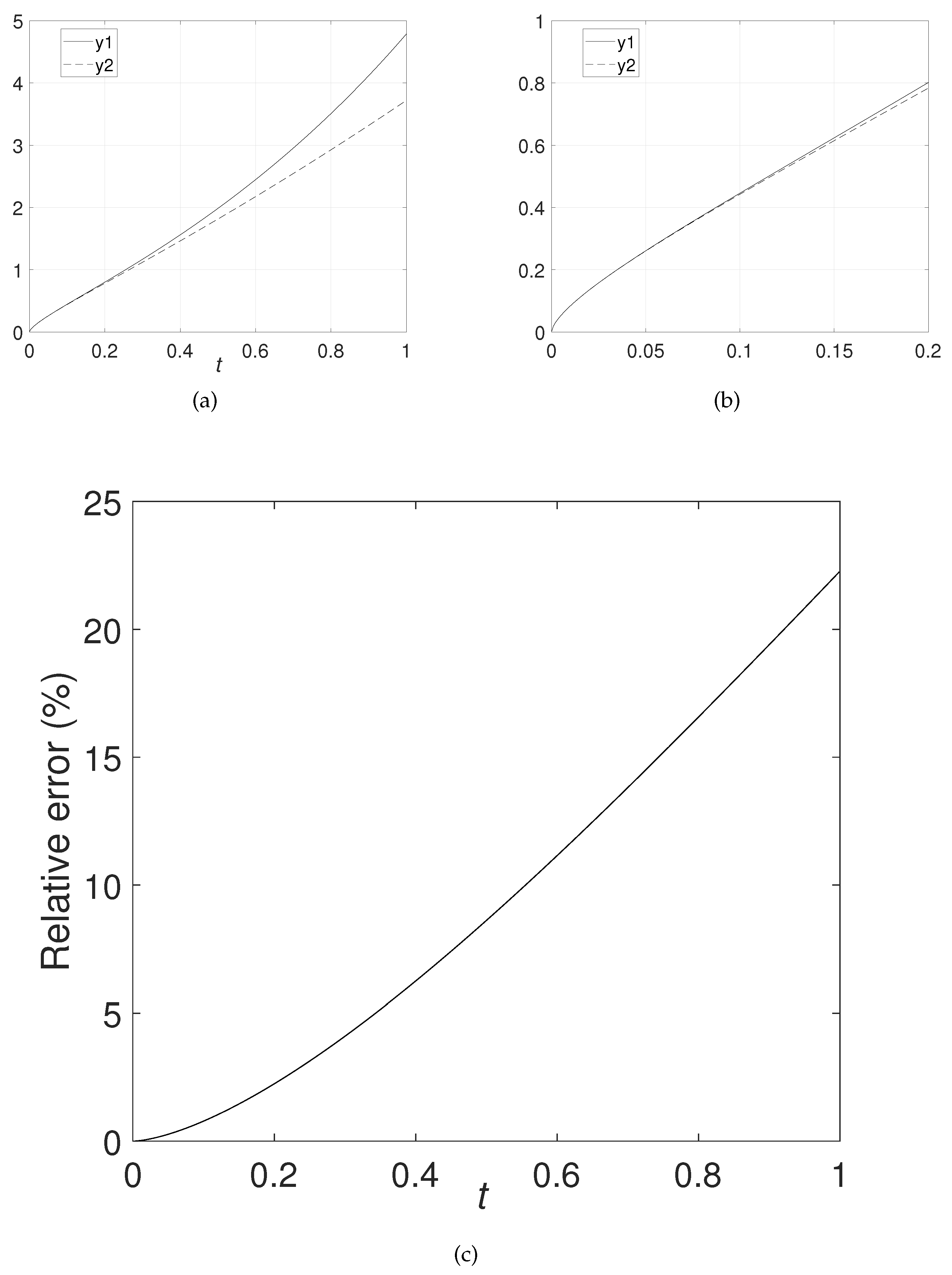
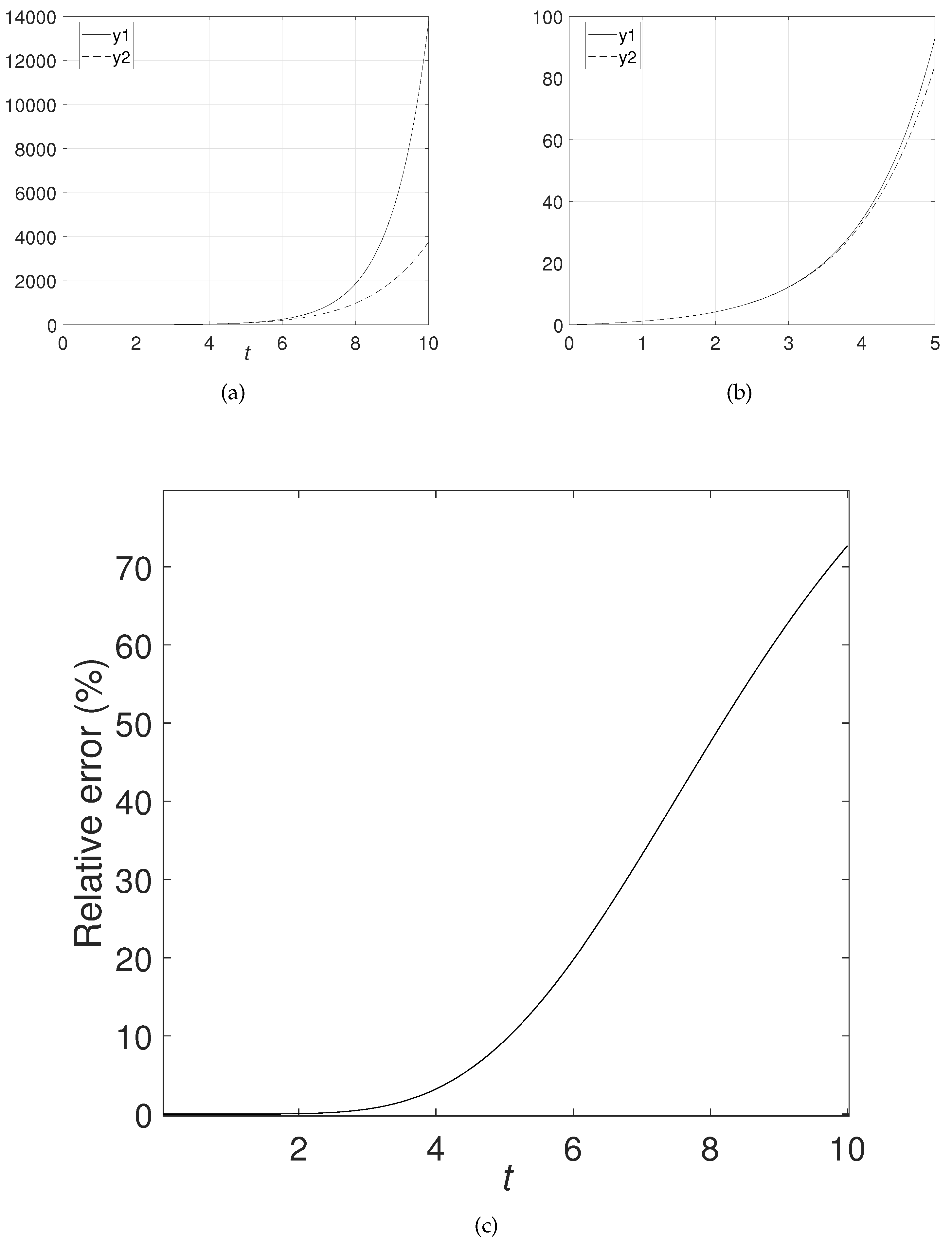
We define y 1 = ς ( t ) , y 2 = ς ˜ n ( t ) , where n = 4 , and use numerical simulation. The numerical simulation results are shown in Figure 1 with ϵ = 0.5 , Figure 2 with ϵ = 0.2 , and Figure 3 with ϵ = 0.8 . The results of the numerical simulations show that the absolute error and the relative error have high accuracy within a certain time range, but quickly diverge beyond this time range and may become misleading.
Example 2.
Suppose that ς ( t ) = k = 0 t 2 k ϵ + 1 Γ ( 1 + 2 k ϵ ) ; then, the n-order approximate expansion is expressed as
ς ˜ n ( t ) = k = 0 n t 2 k ϵ + 1 Γ ( 1 + 2 k ϵ ) .
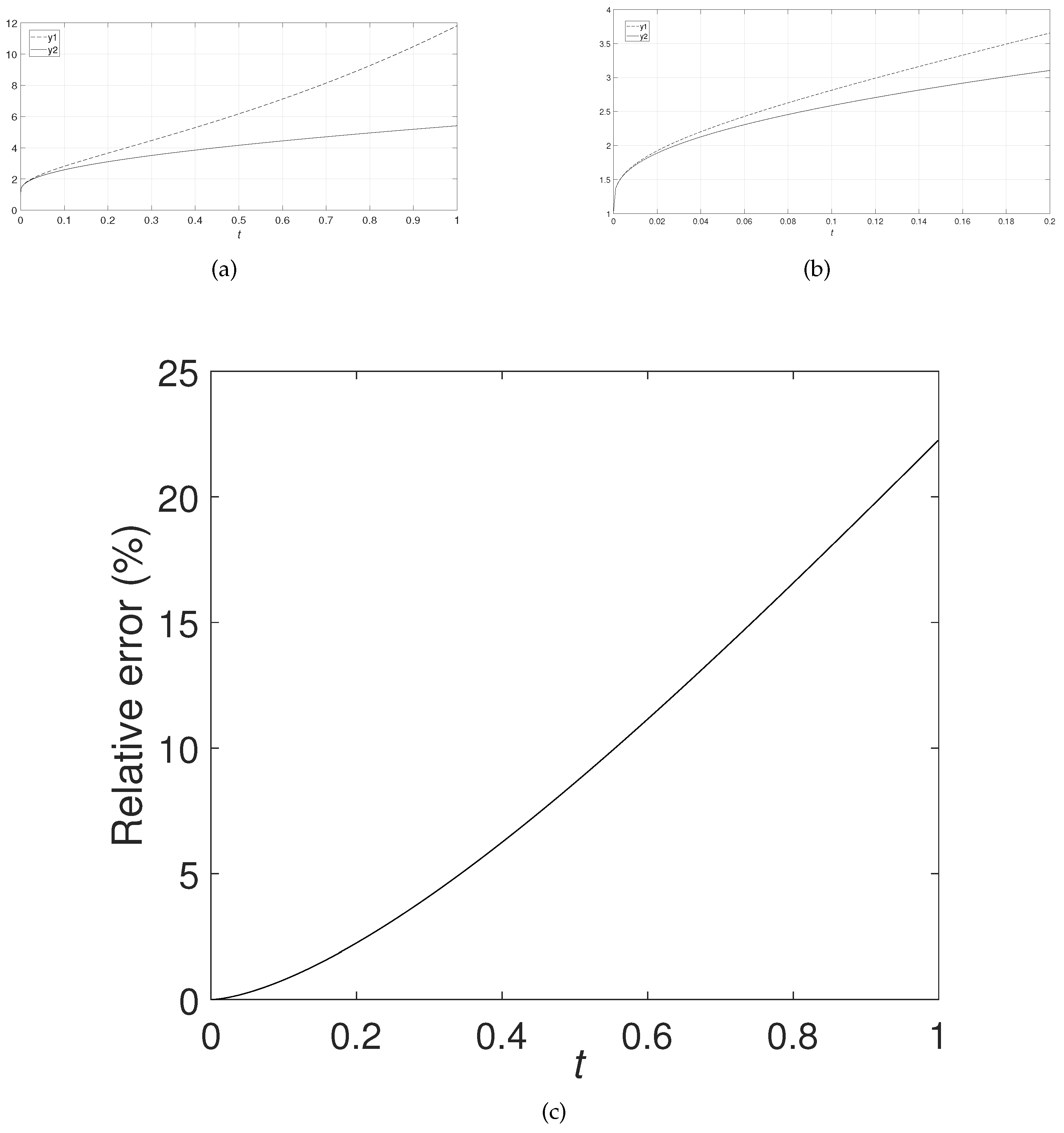
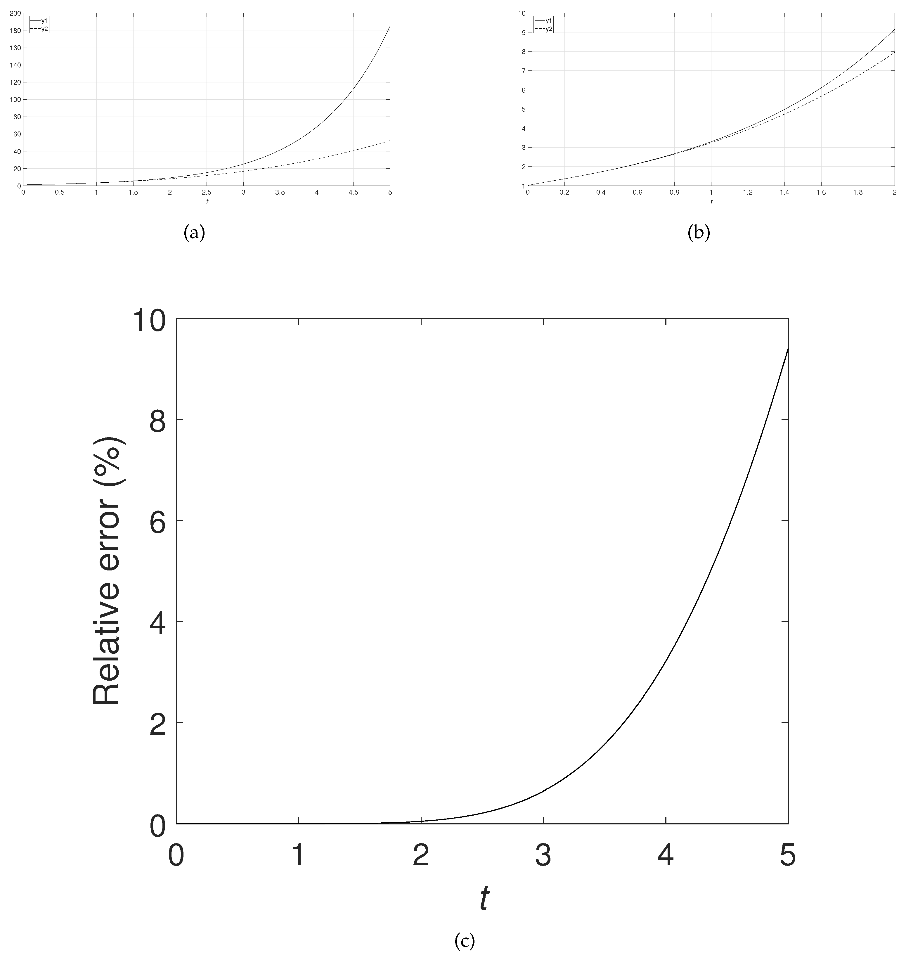
Similarly, we let y 1 = ς ( t ) , y 2 = ς ˜ n ( t ) where n = 4 and use numerical simulation. The numerical simulation results are shown in Figure 4 with ϵ = 0.5 , Figure 5 with ϵ = 0.2 , and Figure 6 with ϵ = 0.8 . The results of the simulations again show that the absolute error and the relative error both have high accuracy within a certain time range, but quickly diverge and become misleading outside of this time range.
The numerical simulations in the above examples verify our theoretical analysis. The aforementioned method can only be applied within a certain time range. Beyond this range, it may be misleading.
Figure 4. The absolute error (a,b) and relative error (c) in Example 2 with ϵ = 0.5 .
Symmetry 16 00912 g004
Figure 5. The absolute error (a,b) and relative error (c) in Example 2 with ϵ = 0.2 .
Symmetry 16 00912 g005
Figure 6. The absolute error (a,b) and relative error (c) in Example 2 with ϵ = 0.8 .
Symmetry 16 00912 g006

6. Conclusions

In this paper, we have presented a detailed analysis of the fractional reduced differential transform method. Theoretical analysis and numerical simulations both show that this method can only be applied within a certain time range and that an applicable condition exists. Thus, for this method, we first need to know the time range and the applicable condition. The mentioned approach can only be studied within this applicable condition (time range); beyond this time range, the obtained solutions may be misleading.

Funding

This work was supported by the National Natural Science Foundation of China under Grant No. 61304062.

Data Availability Statement

The datasets analyzed during the current study are available from the corresponding author on reasonable request.

Conflicts of Interest

The author declares no conflicts of interest.

References

  1. Zhao, L. Comments on “Finite-Time Control of Uncertain Fractional-Order Positive Impulsive Switched Systems with Mode-Dependent Average Dwell Time”. Circuits Syst. Signal Process. 2020, 39, 6394–6397. [Google Scholar] [CrossRef]
  2. Zhao, L. A note on “Cluster synchronization of fractional-order directed networks via intermittent pinning control”. Phys. A-Stat. Mech. Its Appl. 2021, 561, 125150. [Google Scholar] [CrossRef]
  3. Shan, W.; Wang, Y.; Tang, W. Fractional Order Internal Model PID Control for Pulp Batch Cooking Process. J. Chem. Eng. Jpn. 2023, 56, 2201288. [Google Scholar] [CrossRef]
  4. Bishehniasar, M.; Salahshour, S.; Ahmadian, A.; Ismail, F.; Baleanu, D. An Accurate Approximate-Analytical Technique for Solving Time-Fractional Partial Differential Equations. Complexity 2017, 2017, 8718209. [Google Scholar] [CrossRef]
  5. Abdollahi, R.; Khastan, A.; Nieto, J.J.; Rodriguez-Lopez, R. On the linear fuzzy model associated with Caputo-Fabrizio operator. Bound. Value Probl. 2018, 1–18. [Google Scholar] [CrossRef]
  6. Alam Khan, N.; Abdul Razzaq, O.; Riaz, F.; Ahmadian, A.; Senu, N. Dynamics of fractional order nonlinear system: A realistic perception with neutrosophic fuzzy number and Allee effect. J. Adv. Res. 2021, 32, 109–118. [Google Scholar] [CrossRef] [PubMed]
  7. Ahmadian, A.; Salahshour, S.; Ali-Akbari, M.; Ismail, F.; Baleanu, D. A novel approach to approximate fractional derivative with uncertain conditions. Chaos Solitons Fractals 2017, 104, 68–76. [Google Scholar] [CrossRef]
  8. Singh, S.; Ray, S.S. Higher-order approximate solutions of fractional stochastic point kinetics equations in nuclear reactor dynamics. Nucl. Sci. Tech. 2019, 30, 49. [Google Scholar] [CrossRef]
  9. Bohaienko, V.; Bulavatsky, V. Simplified Mathematical Model for the Description of Anomalous Migration of Soluble Substances in Vertical Filtration Flow. Fractal Fract. 2020, 4, 20. [Google Scholar] [CrossRef]
  10. Salama, F.M.; Hamid, N.N.A.; Ali, N.H.M.; Ali, U. An efficient modified hybrid explicit group iterative method for the time-fractional diffusion equation in two space dimensions. AIMS Math. 2022, 7, 2370–2392. [Google Scholar] [CrossRef]
  11. Jaradat, I.; Alquran, M.; Yousef, F.; Momani, S.; Baleanu, D. On (2+1)-dimensional physical models endowed with decoupled spatial and temporal memory indices. Eur. Phys. J. Plus 2019, 134, 360. [Google Scholar] [CrossRef]
  12. Mukhtar, S.; Abuasad, S.; Hashim, I.; Abdul Karim, S.A. Effective Method for Solving Different Types of Nonlinear Fractional Burgers’ Equations. Mathematics 2020, 8, 729. [Google Scholar] [CrossRef]
  13. Liu, J.G.; Yang, X.J.; Feng, Y.Y.; Cui, P. On the (N+1)-dimensional local fractional reduced differential transform method and its applications. Math. Methods Appl. Sci. 2020, 43, 8856–8866. [Google Scholar] [CrossRef]
  14. Ali, G.; Ahmad, I.; Shah, K.; Abdeljawad, T. Iterative Analysis of Nonlinear BBM Equations under Nonsingular Fractional Order Derivative. Adv. Math. Phys. 2020, 2020, 3131856. [Google Scholar] [CrossRef]
  15. Zhao, L.; Chen, Y. Comments on “a novel approach to approximate fractional derivative with uncertain conditions”. Chaos Solitons Fractals 2022, 154, 111651. [Google Scholar] [CrossRef]
  16. Arshad, M.; Lu, D.; Wang, J. (N + 1)-dimensional fractional reduced differential transform method for fractional order partial differential equations. Commun. Nonlinear Sci. Numer. Simul. 2017, 48, 509–519. [Google Scholar] [CrossRef]
  17. Yu, J.; Jing, J.; Sun, Y.; Wu, S. (n + 1)-Dimensional reduced differential transform method for solving partial differential equations’. Appl. Math. Comput. 2016, 273, 697–705. [Google Scholar] [CrossRef]
  18. Abuasad, S.; Alshammari, S.; Al-rabtah, A.; Hashim, I. Solving a Higher-Dimensional Time-Fractional Diffusion Equation via the Fractional Reduced Differential Transform Method. Fractal Fract. 2021, 5, 168. [Google Scholar] [CrossRef]
  19. Owyed, S.; Abdou, M.A.; Abdel-Aty, A.H.; Alharbi, W.; Nekhili, R. Numerical and approximate solutions for coupled time fractional nonlinear evolutions equations via reduced differential transform method. Chaos Solitons Fractals 2020, 131, 109474. [Google Scholar] [CrossRef]
  20. Maisuria, M.A.; Tandel, P.V.; Patel, T. Solution of Two-Dimensional Solute Transport Model for Heterogeneous Porous Medium Using Fractional Reduced Differential Transform Method. Axioms 2023, 12, 1039. [Google Scholar] [CrossRef]
  21. Mahdy, A.M.S.; Gepreel, K.A.; Lotfy, K.; El-Bary, A. Reduced differential transform and Sumudu transform methods for solving fractional financial models of awareness. Appl. Math.-A J. Chin. Univ. Ser. B 2023, 38, 338–356. [Google Scholar] [CrossRef]
  22. Al-rabtah, A.; Abuasad, S. Effective Modified Fractional Reduced Differential Transform Method for Solving Multi-Term Time-Fractional Wave-Diffusion Equations. Symmetry 2023, 15, 1721. [Google Scholar] [CrossRef]
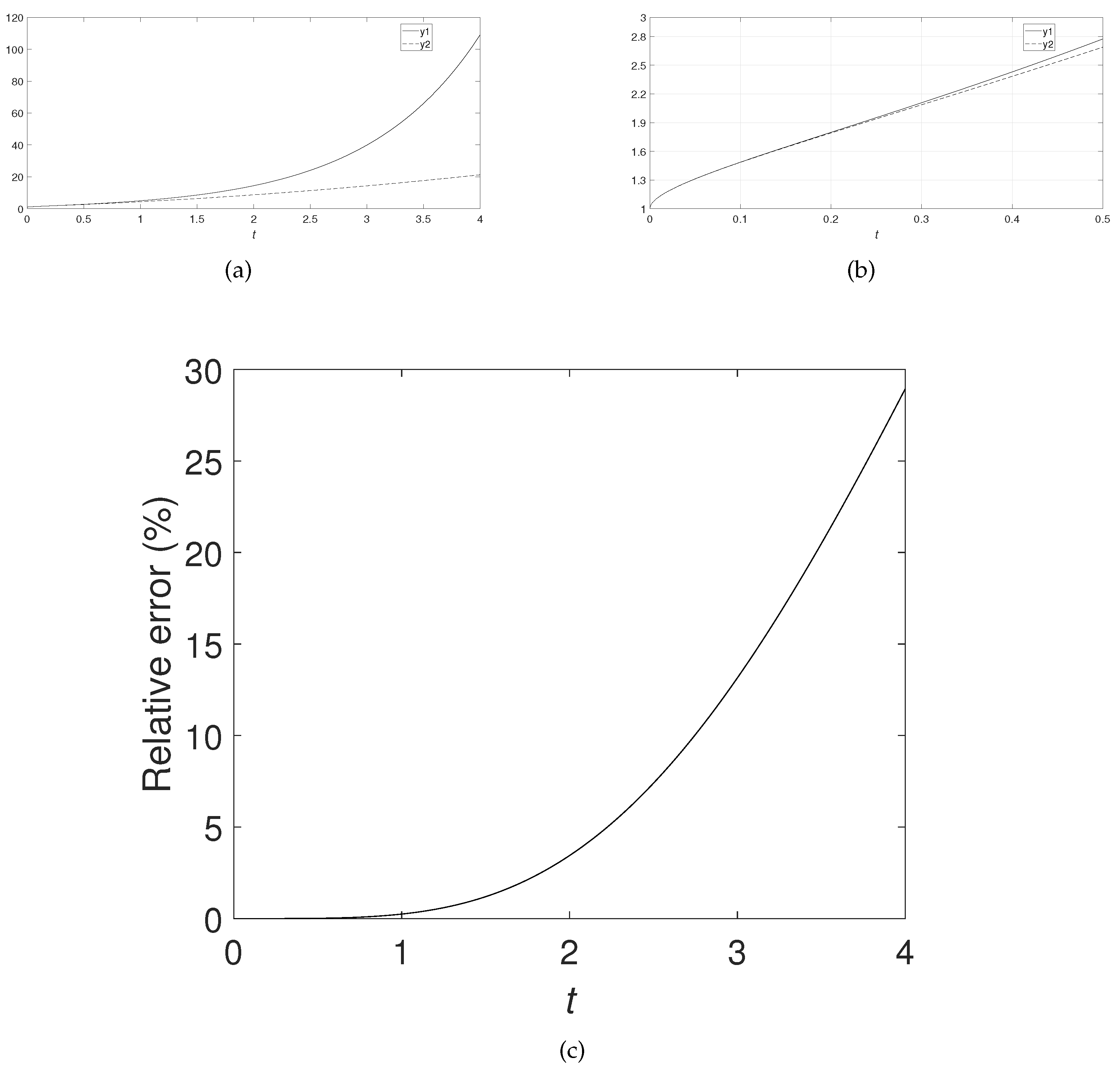
Figure 1. The absolute error (a,b) and relative error (c) in Example 1 with ϵ = 0.5 .
Symmetry 16 00912 g001
Figure 2. The absolute error (a,b) and relative error (c) in Example 1 with ϵ = 0.2 .
Symmetry 16 00912 g002
Figure 3. The absolute error (a,b) and relative error (c) in Example 1 with ϵ = 0.8 .
Symmetry 16 00912 g003
Disclaimer/Publisher’s Note: The statements, opinions and data contained in all publications are solely those of the individual author(s) and contributor(s) and not of MDPI and/or the editor(s). MDPI and/or the editor(s) disclaim responsibility for any injury to people or property resulting from any ideas, methods, instructions or products referred to in the content.