Abstract
This study presents the Hybrid COASaDE Optimizer, a novel combination of the Crayfish Optimization Algorithm (COA) and Self-adaptive Differential Evolution (SaDE), designed to address complex optimization challenges and solve engineering design problems. The hybrid approach leverages COA’s efficient exploration mechanisms, inspired by crayfish behaviour, with the symmetry of SaDE’s adaptive exploitation capabilities, characterized by its dynamic parameter adjustment. The balance between these two phases represents a symmetrical relationship wherein both components contribute equally and complementary to the algorithm’s overall performance. This symmetry in design enables the Hybrid COASaDE to maintain consistent and robust performance across a diverse range of optimization problems. Experimental evaluations were conducted using CEC2022 and CEC2017 benchmark functions, demonstrating COASaDE’s superior performance compared to state-of-the-art optimization algorithms. The results and statistical analyses confirm the robustness and efficiency of the Hybrid COASaDE in finding optimal solutions. Furthermore, the applicability of the Hybrid COASaDE was validated through several engineering design problems, where COASaDE outperformed other optimizers in achieving the optimal solution.
1. Introduction
Optimization, a crucial concept in numerous scientific and engineering fields, aims to improve the efficiency and functionality of systems, designs, or decisions [1]. This interdisciplinary field merges principles from mathematics, computer science, operations research, and engineering to enhance the performance of complex systems [2]. Optimization endeavors to find the optimal values of an objective function within a specified domain, often navigating through competing objectives and constraints [3].
The mathematical backbone of optimization is founded on calculus and linear algebra, enabling the development of sophisticated techniques such as linear programming, quadratic programming, and dynamic programming [4,5]. These methodologies have undergone significant evolution, broadening the scope and applicability of optimization across various sectors, including economics, logistics, network design, and machine learning [6]. However, optimization is most fundamental in algorithm design and analysis, where it enhances efficiency and reduces computational complexity. This is especially critical for managing the large-scale data and complex computations prevalent in the digital era [7]. Similarly, in engineering, optimization plays a vital role in system design to maximize efficiency and minimize costs, with notable applications in aerospace for flight trajectory optimization and in electrical engineering for optimizing circuit designs [8,9].
Moreover, optimization has significantly integrated symmetry in its process, which provides a framework for balancing various algorithmic components to achieve optimal performance [10,11]. In the context of optimization algorithms, symmetry ensures a harmonious integration of different processes such as exploration and exploitation, allowing each phase to contribute equally and effectively to the search for optimal solutions [12,13]. This balanced approach prevents the algorithm from becoming biased towards either extensive searching (exploration) or intensive refining (exploitation), thereby maintaining consistent performance across diverse problem landscapes [14]. By leveraging symmetry, optimization algorithms can navigate complex high-dimensional spaces more efficiently, improving their ability to find global optima while avoiding local traps. Consequently, symmetry is integral to designing robust and versatile optimization algorithms capable of addressing a wide array of engineering and computational challenges [15].
Global optimization techniques that rely on statistical models of objective functions are tailored for tackling “expensive” and “black box” problems. In these scenarios, the limited available information is captured by a statistical model. To handle the high cost associated with such problems, the theory of rational decision-making under uncertainty is particularly appropriate. The resulting algorithms are essentially sequences of decisions made in the face of uncertainty, as informed by the statistical model [16].
Stochastic optimization algorithms are distinguished by their strategic use of randomness to tackle optimization challenges [17]. Unlike deterministic algorithms that follow a strict rule set, stochastic algorithms incorporate probabilistic elements to enhance solution space exploration, proving effective in complex high-dimensional problems with numerous local optima [18,19].
The concept of hybridization in optimization combines multiple optimization strategies to exploit the strengths of individual methods and mitigate their weaknesses, thereby enhancing overall effectiveness [20]. This paper proposes the hybridization of the Crayfish Optimization Algorithm (COA) with the Self-adaptive Differential Evolution (SaDE) technique [21]. COA, known for its global search capability, and SaDE, recognized for its adaptability in adjusting mutation and crossover rates, can be synergized to form a robust hybrid system. This hybrid approach is particularly advantageous in complex landscapes such as engineering design problems, where it provides a dynamic balance between exploration and exploitation, and is adept at handling non-differentiable or discontinuous objective functions in scenarios where traditional methods falter [22].
This hybrid model leverages the randomness of stochastic methods to circumvent the “curse of dimensionality”, in which the solution space grows exponentially with increasing dimensions, making exhaustive searches infeasible [23]. Furthermore, hybrid algorithms can offer more reliable convergence to global optima by navigating efficiently through multiple local optima, allowing them to adapt to various problem settings from machine learning and artificial intelligence to logistics and financial modeling [2].
Hybrid optimization not only consolidates the stochastic elements of methods such as Stochastic Gradient Descent (SGD), Genetic Algorithms (GAs) [24], Particle Swarm Optimization (PSO) [25], and Ant Colony Optimization (ACO) [26], it also introduces versatility in handling discrete and continuous optimization scenarios; discrete hybrid methods are suitable for combinatorial problems such as scheduling, while continuous hybrid strategies are ideal for continuous variable problems such as parameter tuning in machine learning models and optimization in control systems [22]. Thus, the integration of various optimization techniques into a hybrid framework holds the potential to revolutionize the efficiency and applicability of optimization solutions across a broad spectrum of disciplines.
2. Problem Statement
The Self-adaptive Differential Evolution (SaDE) algorithm, despite its powerful adaptive exploitation capabilities, often encounters challenges related to premature convergence. This issue arises due to its intensive local search mechanisms; while efficient at refining solutions, these can sometimes lead to the algorithm becoming trapped in local optima. Conversely, the Crayfish Optimization Algorithm (COA) excels in global search thanks to its explorative strategies inspired by the natural behavior of crayfish. However, COA’s extensive search mechanisms can occasionally lack the precision required for fine-tuning solutions to their optimal values, particularly in complex high-dimensional landscapes.
The selection of SaDE and COA for hybridization is driven by the complementary strengths of these two algorithms. SaDE’s capability to dynamically adjust its parameters during the optimization process makes it highly adaptable and effective at exploitation and refining solutions to a high degree of accuracy. Meanwhile, COA’s robust exploration phase ensures a comprehensive search of the solution space that mitigates the risk of premature convergence and enhances the algorithm’s ability to locate global optima.
The decision to hybridize SaDE and COA was based on a thorough analysis of their individual performance characteristics and the specific requirements of engineering design problems. Engineering optimization often involves navigating complex multimodal landscapes with numerous constraints and conflicting objectives. In such scenarios, relying solely on either exploration or exploitation is insufficient. SaDE’s adaptive mechanisms provide a dynamic approach to parameter adjustment, which is critical for maintaining the algorithm’s responsiveness to different stages of the optimization process. This adaptability ensures that the exploitation phase is finely tuned to the evolving landscape of the problem.
COA’s exploration phase, inspired by the natural foraging behavior of crayfish, introduces a diverse set of candidate solutions into the search space. This diversity is essential for avoiding local optima and ensuring a broad search that can uncover high-quality solutions across the entire solution space. The hybrid COASaDE optimizer leverages the strengths of both algorithms, creating a balanced approach that enhances both exploration and exploitation. This balance is crucial for addressing the complex and varied challenges posed by engineering design problems while ensuring that the optimizer is both versatile and robust.
In light of the diverse and complex nature of engineering design problems, a hybrid approach that balances exploration and exploitation is essential. Many metaheuristic algorithms have been proposed over the years, each with its own unique strengths and weaknesses. However, the strategic combination of COA’s explorative power and SaDE’s adaptive exploitation creates a synergistic effect that enhances the overall performance of the optimization process. This hybrid model is particularly well-suited for engineering applications, where both global search capabilities and local refinement are crucial for efficiently finding high-quality solutions.
In addition, the hybridization of SaDE and COA is a strategic choice aimed at overcoming the limitations of each algorithm when used in isolation. By combining their strengths, the Hybrid COASaDE optimizer provides a powerful tool for solving complex engineering design problems, demonstrating superior performance and reliability across a wide range of benchmark tests and real-world applications.
2.1. Paper Contribution
The primary contributions of this paper are summarized as follows:
- Novel hybrid optimization algorithm: We propose the Hybrid COASaDE optimizer, a strategic integration of the Crayfish Optimization Algorithm (COA) and Self-adaptive Differential Evolution (SaDE). This hybridization leverages COA’s explorative efficiency, characterized by its unique three-stage behaviour-based strategy, and SaDE’s adaptive exploitation abilities, marked by dynamic parameter adjustment. The novelty of this approach lies in the balanced synergy between COA’s broad search capabilities and SaDE’s fine-tuning mechanisms, resulting in an optimizer that excels at both exploration and exploitation.
- Enhanced balance between exploration and exploitation: The Hybrid COASaDE algorithm effectively addresses the balance between exploration and exploitation, a common challenge in optimization. It begins with COA’s exploration phase, which extensively probes the solution space to avoid premature convergence. As potential solutions are identified, the algorithm transitions to SaDE’s adaptive mechanisms, which fine-tune these solutions through self-adjusting mutation and crossover processes. This seamless transition ensures that the algorithm can robustly navigate complex high-dimensional landscapes while maintaining a balanced and effective search process throughout the optimization.
- Engineering applications: The applicability and effectiveness of the Hybrid COASaDE optimizer are validated through several engineering design problems, including welded beam, pressure vessel, spring, speed reducer, cantilever, I-beam, and three-bar truss designs. In each case, Hybrid COASaDE achieves high-quality solutions with improved convergence speeds. This demonstrates the optimizer’s versatility and robustness, making it a valuable tool for a wide range of engineering applications.
2.2. Paper Structure
The rest of this paper is organized as follows. The Introduction outlines the research problem, significance, and main contributions. The Related Work section reviews existing optimization algorithms, focusing on COA and SaDE. Next, overviews of COA and SaDE detail their respective strategies and mechanisms. The Proposed Hybrid COASaDE Optimizer section introduces the integration of COA and SaDE. The Mathematical Model of Hybrid COASaDE section provides detailed mathematical formulations. The Experimental Results section presents benchmark evaluations and comparisons. The Diagram Analysis section includes convergence curves, search history plots, and statistical analyses. The Engineering Problems section demonstrates the optimizer’s application to engineering design problems. Finally, the Conclusion summarizes our findings and suggests future research directions.
3. Related Work
Optimization techniques have seen extensive evolution across various disciplines, significantly driven by developments in mathematics, computer science, operations research, and engineering [27]. These advancements have led to critical enhancements in linear programming, quadratic programming, and dynamic programming, facilitating complex problem-solving across such diverse fields as economics, logistics, and machine learning [3,5,28].
The authors of [29] introduced an enhanced version of the Quantum-inspired Differential Evolution global optimization (QDE) algorithm called EMMSIQDE. EMMSIQDE incorporates a novel differential mutation strategy to improve search and descent capabilities, and employs a multipopulation mutation evolution mechanism to maintain population diversity and independence. Additionally, a feasible solution space transformation strategy is utilized to optimize the solution mapping process. Comparative evaluations on multidimensional unimodal and multimodal functions demonstrated that EMMSIQDE outperforms DE, QDE, QGA, and MSIQDE in terms of optimization ability, scalability, efficiency, and stability.
In [30], the authors introduced WOASCALF, a novel hybrid algorithm combining the Whale Optimization Algorithm (WOA) and the Sine Cosine Algorithm (SCA) with Levy flight distribution to address optimization problems, in particular for high-dimensional problems. WOA excels in exploration but has weaknesses in exploitation, while SCA also faces exploitation issues. The hybrid WOASCALF algorithm leverages the strengths of both algorithms and to improve search agent movement through Levy flight. Evaluations using 23 benchmark functions and three real-world engineering problems showed that WOASCALF outperforms other algorithms in exploration ability.
An enhanced Particle Swarm Optimization (PSO) algorithm named TO-PSO, which uses a quasi-random sequence (QRS) for population initialization to improve the convergence rate and diversity, was proposed in [31]. By incorporating a low-discrepancy sequence, namely, the torus sequence, into PSO for swarm initialization, this approach aims to more effectively address optimization problems. Evaluations on fifteen well known unimodal and multimodal benchmark test problems demonstrated that TO-PSO significantly outperforms traditional PSO, Sobol Sequence-initialized PSO (SO-PSO), and Halton sequence-initialized PSO (HO-PSO) in terms of cost function value, convergence rate, and diversity.
The authors of [32] introduced the Whale Optimization with Seagull Algorithm (WSOA), a hybrid algorithm designed to address the computational accuracy and premature convergence issues of the Seagull Optimization Algorithm (SOA). By combining the contraction-surrounding mechanism of the WOA with the spiral attack behaviour of SOA and incorporating a Levy flight strategy, the WSOA enhances the balance between exploration and exploitation. Evaluations using 25 benchmark test functions and comparisons with seven well known metaheuristic algorithms demonstrated WSOA’s superior performance. Additionally, four engineering examples validated its effectiveness and feasibility.
In [33], the authors proposed a Memory-based Hybrid Crow Search Algorithm (MHCSA) combining the Crow Search Algorithm (CSA) and PSO to address CSA’s limitations in memory representation and balancing exploration and exploitation. By initializing the memory element with PSO’s best solution (pbest) and enhancing CSA’s individuals’ positions using both the global best (gbest) and pbest of PSO, the MHCSA improves diversity and search abilities. Adaptive functions replace CSA’s fixed flight length and awareness probability to better balance exploration and exploitation. When tested on seventy-three benchmark functions and seven engineering design problems, MHCSA demonstrated superior performance, while eliminating early convergence and improving both accuracy and stability, ranking first among CSA, PSO, and other robust methods.
In [34], the authors introduced MBFPA, a hybrid metaheuristic algorithm combining the Butterfly Optimization Algorithm (MVO) and Flower Pollination Algorithm (FPA) based on a mutualism mechanism. While effective, MVO often faces issues with local optimality and premature convergence. The MBFPA enhances exploration through FPA and improves exploitation via symbiosis organism search in the mutualism phase, thereby accelerating convergence. Meanwhile, its adaptive switching probability balances exploration and exploitation. When evaluated on 49 standard test functions, MBFPA outperformed six basic and five hybrid metaheuristic algorithms. Additionally, it successfully solved five classic engineering problems, demonstrating feasibility, competitiveness, and strong application prospects.
The COA, despite its simplicity and innovation, suffers from reduced search efficiency and susceptibility to local optima in later stages. To address these issues, a modified version called MCOA, was proposed in [35]. The MCOA incorporates an environmental renewal mechanism to guide crayfish to better environments based on water quality factors along with a learning strategy based on ghost antagonism to avoid local optima. Performance evaluations using the IEEE CEC2020 benchmark function, four constrained engineering problems, and feature selection problems demonstrated significant improvements. The MCOA showed a 55.23% improvement in average fitness value and a 10.85% increase in accuracy for feature selection problems. The combination of these enhancements substantially boosts MCOA’s optimization performance, offering valuable advancements in solving complex spatial and practical problems.
A modified COA incorporating a Gaussian Distribution (GD) parameter to assess and enhance population and fitness diversity was proposed by the authors of [36]. Their proposed method aims to improve solution quality and robustness in complex optimization environments. The performance of the proposed method was validated by optimizing 27 unimodal and multimodal benchmark functions, showing that the proposed method is more effective and efficient than the traditional COA in fewer iterations.
All of these studies underscore the necessity for enhancing optimization algorithms in order to address their inherent limitations, with a particular focus on the Crayfish Optimization Algorithm (COA). These investigations highlight the critical need for improved search efficiency, preventing premature convergence, and bolstering exploration capabilities to achieve more robust and effective optimization performance. The modifications and hybrid approaches proposed in these studies demonstrate significant advancements in overcoming the shortcomings of traditional algorithms, paving the way for more efficient and reliable solutions to complex optimization problems.
3.1. Overview of COA
The Crayfish Optimization Algorithm (COA) [37] is an innovative metaheuristic algorithm inspired by the foraging behavior of crayfish in nature. At its core, COA is structured around three distinct behavioral stages, each mimicking a specific aspect of the crayfish’s life cycle: the summer resort stage for exploration, the competition stage for resource allocation, and the foraging stage for exploitation. The summer resort stage symbolizes the search for a cooler habitat, guiding the algorithm to explore diverse regions of the solution space to prevent premature convergence. The competition stage, in which crayfish contest for resources, reflects the algorithm’s ability to intensify the search in promising areas. Finally, the foraging stage, akin to crayfish seeking food, represents the fine-tuning of solutions in the algorithm. A unique feature of the COA is its temperature-based mechanism, which controls the transitions between these stages, enabling the algorithm to adaptively balance exploration and exploitation based on the problem’s landscape [37].
3.2. Overview of Self-Adaptive Differential Evolution (SaDE)
Self-adaptive Differential Evolution (SaDE) [38] is a variant of the traditional Differential Evolution (DE) algorithm augmented with a self-adapting mechanism to dynamically adjust its strategy parameters during the optimization process [38]. This enhancement addresses a crucial challenge in DE, namely, the selection of appropriate control parameters such as the scaling factor and crossover rate, which significantly influences the algorithm’s performance. SaDE introduces a learning strategy that allows it to adaptively modify these parameters based on the ongoing success rate of trial vectors in the population. By analyzing the performance feedback from previous iterations, SaDE can effectively tune its mutation and crossover strategies, thereby improving its ability to navigate through complex optimization landscapes [38]. This self-adaptive nature empowers SaDE to maintain a delicate balance between exploration and exploitation, thereby enhancing its efficiency and effectiveness in finding global optima, particularly in complex multimodal optimization scenarios. The adaptability of SaDE makes it a robust and versatile choice for a wide array of optimization problems, allowing it to serve as a foundation for the development of more sophisticated and efficient metaheuristic algorithms [39].
4. Hybrid COASaDE Optimizer
This section introduces the COASaDE Hybrid Optimizer, which combines the Crayfish Optimization Algorithm (COA) with Self-Adaptive Differential Evolution (SaDE). The hybridization approach in our study strategically integrates COA and SaDE to leverage their distinctive strengths and address complex optimization challenges effectively.
The integration process merges the explorative efficiency of COA, known for its unique three-stage behavior-based strategy, with the adaptive exploitation abilities of SaDE, characterized by dynamic parameter adjustment. The hybrid algorithm initiates with COA’s exploration phase by extensively probing the solution space to prevent premature convergence. As potential solutions are identified, the algorithm transitions to employing SaDE’s adaptive mechanisms, which fine-tune these solutions through self-adjusting mutation and crossover processes.
This methodology ensures a comprehensive exploration followed by an efficient exploitation phase, with each algorithm complementing the other’s limitations. The primary challenge in this hybridization lies in achieving a seamless transition between the algorithms while maintaining a balance that allows the strengths of COA and SaDE to synergistically enhance the search process while mitigating their respective weaknesses.
4.1. COASaDE Mathematical Model
- Population Initialization:
The algorithm initializes the population within the search space boundaries using uniformly distributed random numbers. This ensures diverse starting points for the search process, which increases the chance of finding the global optimum, as shown in Equation (1):
where is the i-th individual’s position in the initial population, and are the lower and upper boundaries of the search space, and is a vector of uniformly distributed random numbers.
- 2.
- Evaluation:
Each individual’s fitness is evaluated using the objective function. This step determines the quality of the solutions, guiding the search process, as shown in Equation (2):
where is the objective function and is the fitness of the i-th individual.
- 3.
- Mutation Factor and Crossover Rate Initialization:
The algorithm initializes the mutation factor and crossover rate uniformly for all individuals. This provides a balanced exploration and exploitation capability initially, as shown in Equation (3):
where is the mutation factor and is the crossover rate for the i-th individual.
- 4.
- Adaptive Update:
The mutation factor and crossover rate are updated adaptively based on past success, enhancing the algorithm’s ability to adapt to different optimization landscapes dynamically, as shown in Equations (4) and (5):
where represents a normal distribution with mean and standard deviation .
- 5.
- COA Behavior:
The algorithm applies COA-specific behaviours such as foraging and competition based on temperature, which helps to diversify the search process and avoid local optima, as shown in Equations (6) and (7):
where is the decreasing factor, is a random vector, is the food position, and is a randomly chosen individual’s position.
- 6.
- SaDE Mutation and Crossover:
Differential Evolution’s mutation and crossover mechanisms are applied to generate trial vectors, promoting solution diversity and improving the exploration capabilities of the algorithm, as shown in Equations (8) and (9):
where are distinct indices different from i, is the mutant vector, is the trial vector, is a random number, and is a randomly chosen index.
- 7.
- Selection:
The fitness of the trial vectors is evaluated and individuals are updated if the new solution is better. This step ensures that only improved solutions are carried forward, enhancing convergence towards the optimum, as shown in Equations (10) and (11):
where is the updated position of the i-th individual and is its fitness.
- 8.
- Final Outputs:
The best solution found is returned as the final result along with the convergence curve indicating the algorithm’s performance over time, as shown in Equations (12) and (13):
where is the best solution found, is its fitness, and is the best fitness at each iteration t.
The Hybrid Crayfish Optimization Algorithm with Self-Adaptive Differential Evolution (COASaDE) combines the Crayfish Optimization Algorithm’s behavior with the evolutionary strategies of Differential Evolution (DE). The algorithm begins by initializing the population, mutation factor, and crossover rate. It then evaluates the initial population’s fitness to determine the best solution. As the iterations proceed, when the iteration count exceeds a predefined stabilization period, the mutation factor and crossover rate are adaptively updated based on past success. The COA parameters, including the decreasing factor and temperature, are updated as well. Depending on the temperature, either the COA foraging/competition behaviour or DE mutation and crossover are performed. The algorithm evaluates new positions and updates the individuals when improvements are found. The global best position and fitness are updated at each iteration. The process continues until the stopping criterion is met, at which point the algorithm returns the best fitness and position along with the convergence information. The flowchart visualizes these steps, starting from initialization and moving through population evaluation, parameter updates, behavioural checks, mutation/crossover processes, evaluation of new positions, and updating global bests before concluding with the final results. Each decision point and process in the flowchart is linked to specific equations that define the algorithm’s operations. Please see Algorithm 1.
| Algorithm 1 Pseudocode for the Hybrid COASaDE algorithm. |
|
4.2. Exploration Phase of Hybrid COASaDE
The exploration phase of COASaDE is critical for navigating the search space and uncovering potential solutions. This phase leverages the exploration capabilities of COA combined with the adaptive mutation and crossover mechanisms of SaDE to effectively balance exploration and exploitation. The algorithm employs diverse strategies, including the foraging, summer resort, and competition stages, to facilitate varied movement patterns among candidate solutions while adapting to environmental cues for efficient search space exploration. Adaptive parameter adjustment plays a significant role in this phase by dynamically fine-tuning the mutation factors (F) and crossover rates () for a subset of the population. This adjustment ensures that the algorithm adapts to changing conditions and maintains an effective balance between exploration and exploitation based on solution performance. Additionally, randomization and diversity maintenance are crucial, as is the introduction of stochasticity to prevent premature convergence to suboptimal solutions. By incorporating random factors such as temperature conditions and individual selection for parameter adaptation, the algorithm maintains diversity within the population, preventing it from becoming stuck in local optima and ensuring comprehensive exploration of the search space.
4.3. Exploitation Phase of Hybrid COASaDE
The exploitation phase of the hybrid Crayfish Optimization Algorithm with Self-Adaptive Differential Evolution (see Figure 1) focuses on refining candidate solutions to enhance their quality and convergence towards optimal solutions. This phase utilizes the adaptive mutation and crossover mechanisms of SaDE to efficiently exploit promising regions of the search space. The algorithm leverages the refined candidate solutions from the exploration phase and applies mutation and crossover operations to iteratively improve them. Boundary handling ensures that the solutions remain within the defined search space, preventing the generation of infeasible solutions and maintaining optimization integrity. Fitness evaluation and updating are pivotal, as newly generated solutions are evaluated using the objective function and superior solutions replace their parents in the population. The exploitation phase operates iteratively over multiple generations, refining candidate solutions based on evaluation of the objective function. Through continuous updates based on mutation, crossover, and fitness, COASaDE converges towards optimal or near-optimal solutions, effectively exploiting the promising regions identified during the exploration phase.
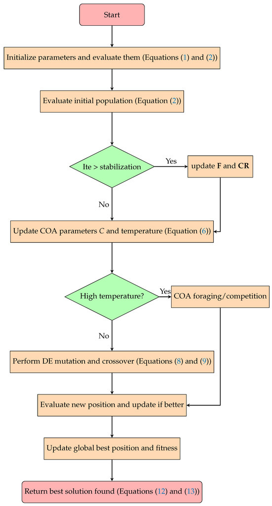
Figure 1.
Flowchart of the proposed Hybrid COASaDE algorithm.
4.4. Solving Global Optimization Problems Using COASaDE
Global optimization problems involve finding the best possible solution from all feasible solutions, often in the presence of complex constraints and multiple local optima. These problems are characterized by their “black box” nature, where the objective function and constraints might not have explicit forms, making traditional analytical methods impractical [16]. Instead, heuristic and metaheuristic algorithms such as Differential Evolution, Genetic Algorithms, and Hybrid Optimization techniques are employed to efficiently navigate the search space. These algorithms iteratively explore and exploit the solution space, aiming to converge on the global optimum despite the challenges posed by the problem’s landscape [40].
The general formulation of a global optimization problem can be expressed mathematically. This involves defining an objective function to be minimized or maximized and specifying the constraints that the solution must satisfy. The objective function, denoted as , and the constraints are illustrated in Equation (14):
where:
is the vector of decision variables, is the objective function, for are the inequality constraints, and for are the equality constraints.
4.5. Symmetry in Hybrid COASaDE
The novel Hybrid COASaDE algorithm represents a fusion of mathematical theory and heuristic strategies, showcasing remarkable symmetry in its approach to optimization. Inspired by crayfish foraging behavior, COASaDE combines local and global search capabilities with heuristic rules derived from natural behaviors, effectively guiding the search process. The Differential Evolution (DE) framework, which underpins SaDE, uses mathematical models for differential mutation and crossover to explore the search space, while its self-adaptive mechanism adjusts control parameters dynamically based on the current optimization state. This hybrid optimizer balances exploration and exploitation by incorporating mathematical models and adaptive heuristics in order to use population-based search mechanisms to evolve candidate solutions. The synergy between COA’s random and directed movements and SaDE’s differential evolution framework enhances both global optimization and local search adaptability. This integration leverages the strengths of both algorithms, combining rigorous mathematical foundations with adaptive, nature-inspired heuristics to effectively solve complex optimization problems.
4.6. Computational Complexity of COASaDE
The computational complexity of COASaDE is influenced by several factors inherent to both Crayfish Optimization Algorithm (COA) and Self-Adaptive Differential Evolution (SaDE) that remain when combining them in a hybrid approach.
4.7. Computational Components
- Initialization:The population X is initialized with N individuals (Equation (15)), where D is the dimensionality of the search space.
- Fitness evaluation:The fitness of each individual in X is evaluated, where M is the complexity of the objective function.
- Adaptive parameter updating:The adaptive parameters F and for individuals are periodically updated, typically at every tenth iteration beyond .
- COA and SaDE operations:This controls COA behaviors (Equation (18)) and alternative COA behaviors (if condition ).This controls SaDE mutation and crossover operations (Equation (19)).
- Boundary conditions and fitness updating:This is used to apply the boundary conditions.This is used to evaluate the fitness of mutated individuals.
- Termination:The algorithm runs for T iterations, with T directly influencing the total computational complexity.
The computational complexity of COASaDE per iteration is primarily governed by the population size N, the dimensionality of the problem space D, the complexity of the objective function M, and the number of iterations T. The proposed hybrid approach aims to efficiently tackle complex optimization problems by combining adaptive parameter control and diverse search strategies from COA and SaDE.
5. Testing and Comparison
In our experimental testing and evaluation of COASaDE, we aimed to validate its efficacy and performance against a series of challenging benchmark functions. This section presents a comprehensive analysis of the results obtained from testing COASaDE on the CEC2017 and CEC2022 benchmark suites. The analysis involved comparing the performance of COASaDE with several state of art optimization algorithms. The comparative study focused on various metrics such as convergence speed, accuracy, robustness, and ability to escape local optima, providing a clear perspective on the strengths and potential limitations of the proposed COASaDE algorithm.
The selection of these algorithms was driven by several key considerations. First was the aim of representing a diverse range of optimization techniques. Algorithms such as GWO, PSO, MFO, MVO, SHIO, AOA, FOX, FVIM, and SCA embody different paradigms, from evolutionary and swarm intelligence-based methods to physics-inspired and hybrid approaches. This diversity allows researchers to conduct a comprehensive evaluation of COASaDE against established benchmarks to ensure a thorough exploration of its relative strengths and weaknesses across varied optimization scenarios.
Moreover, the choice of algorithms was guided by their status as benchmark standards within the optimization community. Algorithms such as WOA, GWO, and SCA have been extensively studied and cited, and as such can provide a reliable basis for comparison against newer or hybrid approaches like COASaDE. By benchmarking against well known algorithms, researchers can more effectively assess the performance of COASaDE, contributing to a deeper understanding of its capabilities and potential advancements in optimization research.
5.1. CEC2022 Benchmark Description
The CEC2022 benchmark suite represents a critical development in the field of optimization, focusing on single-objective and bound-constrained numerical optimization problems (see Figure 2). As a part of the evolutionary progression from previous competitions such as CEC’05 through CEC’21, which focused on real-parameter optimization, the CEC2022 suite introduces challenges based on substantial feedback from the CEC’20 suite. This feedback has been instrumental in refining the problem definitions and evaluation criteria in order to better assess the capabilities of modern optimization algorithms such as COASaDE.
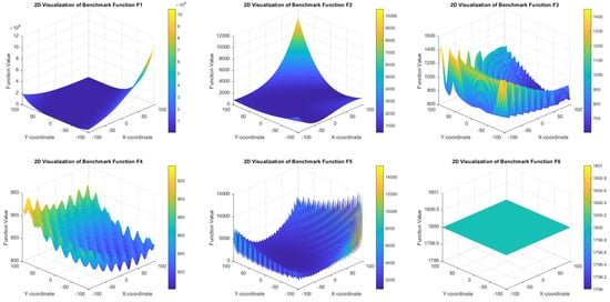
Figure 2.
Illustration of CEC2022 benchmark functions (F1–F6).
Structured to ensure fairness, impartiality, and a reflection of real-world complexities, the CEC2022 benchmarks are suitable for testing the COASaDE optimizer. This suite allows researchers to test their algorithms against cutting-edge methods in a competitive setting that mirrors current industry and academic demands. The CEC 2022 Special Session and Competition on Single-Objective Bound-Constrained Numerical Optimization offers a pivotal platform for the COASaDE optimizer to demonstrate its efficacy and for researchers to identify potential improvements and inspire the development of next-generation optimization technologies.
5.2. CEC2017 Benchmark Description
The CEC2017 benchmark suite serves as an exhaustive testing ground for the proposed COASaDE optimizer, comprising a diverse array of functions that present multifaceted challenges typical of real-world optimization scenarios. This suite includes multimodal landscapes, high-dimensional spaces, and intricate global structures that rigorously test an algorithm’s capability to efficiently explore and exploit the search space. These functions are strategically chosen to mimic real-life problems, ensuring that the insights gleaned from the COASaDE’s performance are relevant and applicable in practical applications.
Each function within the CEC2017 suite is designed to highlight specific challenges, such as navigating extensive flat areas without premature convergence and handling noise that can obscure the true optima. Additionally, the inclusion of rotated and shifted versions of the base functions introduces further complexity, simulating the effects of variable data transformations seen in real-world environments. These features make the CEC2017 benchmarks suitable for assessing the COASaDE optimizer’s precision, scalability, and adaptability across different orientations and problem scales, thereby offering a thorough evaluation of its practical applicability and robustness.
5.3. Configuration of Parameters for CEC Benchmark Evaluations
The parameters utilized for comparing the optimizers are detailed in Table 1. A consistent parameter configuration is crucial for ensuring fair and effective evaluation across the CEC benchmarks from 2022, 2017, and 2014 and for facilitating a standardized testing environment across various functions.

Table 1.
Configuration of parameters across CEC benchmarks.
The parameters listed in Table 1 were adopted to create a balanced framework supporting comparisons across diverse studies, ensuring a comprehensive and rigorous performance assessment of the algorithms. The chosen population size of 100 and problem dimensionality of 30 strike an optimal balance between the computational demand and the complexity required for significant evaluations. The ceiling on function evaluations, defined as 10,000 , provides ample opportunities for the algorithms to demonstrate their efficiency and convergence capabilities over extensive iterations. The fixed search boundary, set from across all dimensions, ensures a vast and uniform exploration space. Finally, specific benchmarks were made more challenging with the application of rotational and shifting transformations to test the adaptability and robustness of algorithms under enhanced complexity conditions.
A comprehensive statistical analysis was employed for the performance evaluation of various optimization algorithms (see Table 2), including calculation of the mean and standard deviation and the application of the Wilcoxon rank-sum test. The mean serves as a measure of the central tendency, representing the average result obtained by the algorithms across multiple trials. In contrast, the standard deviation quantifies the dispersion or variability around this mean, offering insights into the consistency and reliability of the algorithms across different runs.
Table 2.
Parameter settings for the compared algorithms.
To further assess the statistical significance of differences between the performance of two distinct groups of algorithmic outcomes, the Wilcoxon rank-sum test was utilized. This nonparametric test helps to determine whether there is a statistically significant difference between the medians of the two groups, providing a robust method for comparing the performance of optimization algorithms under various conditions.
5.4. CEC2022 Results
The performance of COASaDE on the CEC2022 benchmark suite demonstrates its robustness and superiority compared to several well known and state-of-the-art optimization algorithms. As shown in Table 3, COASaDE consistently ranks highly across various test functions, often achieving the best or near-best mean and standard deviation values. For instance, on Function F1, COASaDE achieves the lowest mean (3.00E+02) and smallest standard deviation (1.42E-04), significantly outperforming other algorithms including GWO, PSO, and MFO, all of which have higher means and larger standard deviations. This trend continues across multiple functions, indicating COASaDE’s ability to maintain stable and high quality solutions. The algorithm’s self-adaptive mechanism for adjusting mutation factors and crossover rates plays a crucial role in its success, enabling it to effectively balance exploration and exploitation. The results suggest that COASaDE’s combination of crayfish-inspired foraging behavior and differential evolution techniques makes it a powerful tool for tackling complex optimization problems.
Table 3.
Comparison results with well known and state-of-the-art optimizers on CEC2022, FES = 1000, Agents = 50.
The performance of COASaDE on the CEC2022 benchmark suite is shown in Table 4, which shows the comparison results with various Differential Evolution (DE) variants. The results highlight its effectiveness and competitiveness, showing that COASaDE consistently ranks among the top performers across multiple test functions. For Function F1, COASaDE achieves the best mean (3.00E+02) and smallest standard deviation (1.42E-04), demonstrating its precision and stability compared to other DE variants such as LDE, BBDE, and JADE, which all have higher means and larger standard deviations. This trend of superior performance continues with Functions F2 and F3, where COASaDE secures the top ranks, indicating its robustness in handling different optimization challenges. COASaDE also performs well on Function F4, showcasing its adaptability, although it ranks slightly behind some variants.
Table 4.
Comparison Results with variant Differential Evolution optimizers on CEC2022, FES = 1000, Agents = 50.
Moreover, the results indicate that COASaDE maintains a strong balance between exploration and exploitation, facilitated by its adaptive mechanisms for mutation and crossover rates. For Functions F6 to F12 COASaDE consistently ranks within the top positions, often securing the first or second rank. The algorithm’s ability to dynamically adjust its parameters based on the current state of the optimization process allows it to effectively navigate the search space and avoid local optima. Additionally, the comparative analysis with DE variants such as SADE, CMAES, and others highlights COASaDE’s competitive edge in terms of mean performance and consistency, as reflected in the values for the standard error of the mean (SEM). Overall, the results from Table 2 underscore COASaDE’s superior optimization capabilities, robust performance, and effectiveness as a hybrid optimizer that successfully integrates heuristic strategies with mathematical rigor.
5.5. Wilcoxon Rank-Sum Test Results
The Wilcoxon rank-sum test results highlight the statistical significance of COASaDE’s performance on the CEC2022 benchmark functions compared to various other optimizers. Across multiple functions in Table 5 and Table 6 (F1 to F12), COASaDE consistently achieves p-values of against most compared optimizers, indicating statistically significant improvement. For example, on Function F1 COASaDE shows significant differences with all listed algorithms, including GWO, PSO, and MFO. On Function F2, while maintaining strong significance against most optimizers, it exhibits less significant results compared to SHIO and slightly higher p-values with AOA and SCA. This pattern is observed across other functions as well, with COASaDE demonstrating robust performance and often outperforming competitors by statistically significant margins. The few instances of higher p-values, such as in F6 with SHIO and SCA and in F10 with GWO and SHIO, suggest areas where the performance differences are less pronounced. Overall, the Wilcoxon test results affirm the effectiveness and reliability of COASaDE in providing superior optimization results across various challenging functions.
Table 5.
Wilcoxon rank-sum test over CEC2022, FES = 1000, Agents = 50.
Table 6.
Wilcoxon rank-sum test over CEC2022, FES = 1000, Agents = 50.
5.6. COASaDE Results on CEC2017
The results of COASaDE on the CEC2017 benchmark suite, shown in Table 7, highlight its strong performance relative to other optimizers. For Function F1, COASaDE achieves the lowest mean value of and ranks first, demonstrating its efficiency in solving this optimization problem compared to other algorithms such as GWO, PSO, and MFO, which have significantly higher mean values. Similarly, on Function F2 COASaDE ranks third with a mean value of , showing competitive performance among the top optimizers. On Function F3, COASaDE excels with a mean value of , securing the third position and outperforming algorithms such as MFO and GWO, both of which rank lower. For Function F4, COASaDE again ranks first, with a mean value of , indicating its robustness and stability. The algorithm continues to perform well on Function F5, ranking first with a mean value of , highlighting its consistent ability to find optimal solutions. The trend of strong performance is evident across other functions as well. For example, on Function F6 COASaDE achieves the top rank with a mean value of . On Function F7, it ranks third with a mean value of , showcasing its competitive edge. On Function F8, COASaDE ranks second with a mean value of , demonstrating its precision and effectiveness.
Table 7.
Comparison test results with different optimizers on CEC2017, FES = 1000, Agents = 50.
On more challenging functions such as F9 and F10, COASaDE maintains its competitive performance, ranking third and second, respectively. Its mean values are for F9 and for F10. This consistency is further evident on Function F11, where COASaDE ranks third with a mean value of , outperforming many other well-known algorithms. For Function F12, COASaDE ranks second with a mean value of , reinforcing its strong optimization capabilities. On Function F13 it ranks third with a mean value of , showcasing its adaptability. On Function F14, COASaDE secures the second position with a mean value of , demonstrating its robustness across diverse optimization problems. Finally, on Function F15 COASaDE ranks fifth with a mean value of , indicating that while it is highly competitive there is still room for improvement in certain complex scenarios.
The performance of COASaDE on CEC2017 functions F16 to F30, shown in Table 8, indicates its strong competitiveness across a variety of optimization problems. For F16, COASaDE ranks first with a mean value of , outperforming all other algorithms, including GWO and PSO. On F17, COASaDE ranks third with a mean value of , demonstrating its consistent performance among the top optimizers. Notably, COASaDE achieves the lowest mean value on F18 with , highlighting its exceptional ability to handle complex optimization scenarios. On F19, COASaDE again secures the top position with a mean of , showcasing its robustness in solving high-dimensional functions. It maintains this trend on F20, ranking second with a mean value of . For F21, COASaDE ranks second with a mean value of , further indicating its reliability. Similarly, COASaDE’s performance in F22 is commendable; it achieves the lowest mean value of , outperforming other algorithms by a significant margin. The trend continues for F23, where COASaDE ranks first with a mean value of , and for F24, where it secures the top rank with a mean of . On F25, COASaDE ranks second with a mean value of , demonstrating its ability to consistently find optimal solutions across different problems. For F26, COASaDE ranks second with a mean value of , confirming its effectiveness in various optimization contexts. On F27, COASaDE ranks first with a mean value of , outperforming other well-known algorithms such as GWO and PSO. For F28, it achieves the lowest mean value of , highlighting its superior performance. COASaDE also excels on F29, securing the top position with a mean value of . Lastly, COASaDE ranks first on F30 with a mean value of , outperforming all other algorithms and demonstrating its capability to effectively handle complex and diverse optimization problems.
Table 8.
Comparison test results with different optimizers on CEC2017 (F16-F30), FES = 1000, Agents = 50.
As can be seen from Table 9, the comparison of COASaDE with other Differential Evolution optimizers on CEC2017 functions F1 to F15 demonstrates strong performance across a variety of optimization problems. For F1, COASaDE ranks second with a mean value of , closely following JADE, which ranks first. On F2, COASaDE ranks third with a mean of , outperformed only by JADE and DEEM. COASaDE achieves the best performance on F3, ranking first with a mean of , demonstrating its efficiency in solving this problem. On F4, COASaDE again secures the top position with a mean value of , indicating its robustness. For F5, COASaDE ranks fifth with a mean of , showing competitive, though not the best performance. COASaDE excels again on F6, ranking first with a mean of , outperforming the other optimizers by a significant margin. COASaDE ranks second on F7 with a mean of , closely following COA. For F8, it ranks fourth with a mean of , demonstrating consistent performance. COASaDE achieves the best result on F9, ranking first with a mean of , further showcasing its effectiveness. On F10, COASaDE ranks third with a mean of , indicating strong performance. For F11, COASaDE ranks fifth with a mean of , demonstrating competitive performance but not the best results. On F12, COASaDE ranks second with a mean of , showing strong performance. For F13, COASaDE ranks second with a mean of , closely following LDE. COASaDE secures the third position on F14 with a mean of , indicating its robustness in solving this problem. Finally, on F15, COASaDE ranks second with a mean of , demonstrating its consistent performance across different optimization scenarios.
Table 9.
Comparison test results with Differential Evolution variant optimizers on CEC2017 (F1–F15), FES = 1000, Agents = 50.
Furthermore, the results in Table 10 for F16 to F30 highlight the competitive performance of COASaDE. For F16, COASaDE ranks third with a mean value of 2250, showing strong performance but slightly behind JADE and DEEM. On F17, COASaDE achieves the best performance, ranking first with a mean of 1990. For F18, COASaDE again secures the top position with a mean of 1.21E+07, outperforming all other optimizers. On F19, COASaDE ranks first with a mean of 408000, demonstrating its effectiveness in solving this problem. For F20, COASaDE ranks second with a mean of 2310, showing strong performance, though not the best. On F21, COASaDE ranks first with a mean of 2390, indicating its robustness. For F22, COASaDE ranks first with a mean of 3070, demonstrating its efficiency. On F23, COASaDE secures the top position with a mean of 2710, outperforming the other optimizers. For F24, COASaDE ranks first with a mean of 2850, showing strong performance. On F25, COASaDE ranks third with a mean of 3550, demonstrating competitive results. For F26, COASaDE ranks third with a mean of 4460, showing a strong but not the best performance. On F27, COASaDE achieves the best performance, ranking first with a mean of 3170. For F28 COASaDE ranks first with a mean of 3620, demonstrating its efficiency. On F29, COASaDE ranks second with a mean of 3670, showing strong performance. Finally, on F30 COASaDE ranks second with a mean of 2.56E+07, indicating competitive results.
Table 10.
Comparison test results with Differential Evolution variant optimizers on CEC2017 (F16–F30), FES = 1000, Agents = 50.
5.7. Wilcoxon Rank-Sum Test Results on CEC2017
As it can be seen in Table 11 and Table 12, the Wilcoxon rank-sum test results for COASaDE reveal notable statistical differences in comparison with other optimizers across the CEC2017 benchmark functions (F1–F30). COASaDE displays significant p-values for many functions, indicating that its performance differs meaningfully from other optimizers. Specifically, for F1, COASaDE shows a p-value of 3.97E-03 when compared to PSO, suggesting a significant difference. On F2, COASaDE exhibits a p-value of 1.11E-05 against MFO, further underscoring a significant performance disparity. Similar results are observed for F3 and F4, with COASaDE showing p-values of 3.97E-03 and 4.55E-04, respectively, against MFO. These significant p–values, which are often lower than 0.05, consistently suggest that COASaDE’s performance is statistically different compared to other optimizers such as PSO, MFO, SHIO, and FOX across various functions.
Table 11.
Wilcoxon rank-sum test results over CEC2017, FES = 1000, Agents = 50.
Table 12.
Wilcoxon rank-sum test results over CEC2017, FES = 1000, Agents = 50.
5.8. Diagram Analysis
5.8.1. Convergence Curve Analysis
The convergence curves of COASaDE, shown in Figure 3 and Figure 4, demonstrate good convergence performance over the CEC2022 benchmark suite of functions F1 to F12. The curves indicate that COASaDE consistently achieves lower best values and converges quickly. For instance, on functions such as F6 and F8 COASaDE rapidly reaches near-optimal solutions within the initial iterations, highlighting its efficiency in exploring and exploiting the search space. The convergence curve for F6 shows COASaDE stabilizing, showcasing its capability in handling complex multimodal functions where local optima are prevalent. Similarly, the curves for F8 and F9 indicate that COASaDE quickly narrows the search down to the optimal regions.

Figure 3.
Convergence curve analysis over selected functions of CEC2022 (F1–F6).
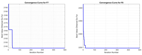

Figure 4.
Convergence curve analysis over selected functions of CEC2022 (F7–F12).
5.8.2. Search History Plot Analysis
The search history plots for the COASaDE algorithm over CEC2022 benchmark functions F1 to F12 (see Figure 5 and Figure 6) illustrate its exploration and exploitation capabilities within the search space. The color gradients represent the objective function values, with lower values indicated by warmer colors (e.g., red) and higher values by cooler colors (e.g., blue). In the search history plots for functions such as F6, F8, and F10, COASaDE demonstrates a focused search pattern, clustering around regions with lower objective function values. This suggests effective exploitation of promising areas, with occasional diversification to explore new regions. For instance, for F6 the red clusters indicate that COASaDE consistently finds and refines solutions within a promising region. Similarly, for F8 and F9 the dense concentration of red and orange points around certain areas highlights COASaDE’s ability to identify and exploit optimal or near-optimal solutions. The search history for F10 shows initial broad exploration followed by a more concentrated search, indicating a balanced exploration–exploitation strategy. Moreover, the search history plots confirm the proficiency of COASaDE in navigating complex landscapes while efficiently balancing exploration of the search space and exploitation of high-quality solutions.

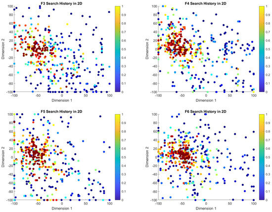
Figure 5.
Search history analysis over selected functions of CEC2022 (F1–F6).
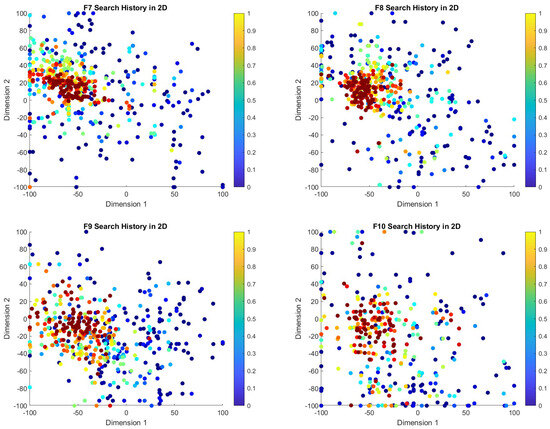

Figure 6.
Search history analysis over selected functions of CEC2022 (F7–F12).
5.8.3. Sensitivity Analysis
As can be seen in Figure 7 and Figure 8, the sensitivity analysis of COASaDE over CEC2022 benchmark functions F1 to F12 reveals notable variations in performance based on the number of search agents and number of maximum iterations. For F1, the performance improves with more iterations and higher numbers of agents, showing optimal performance around 300–400 iterations with 40–50 agents. For F2, the results suggest that higher iterations improve performance, although the results plateau beyond 500 iterations, indicating diminishing returns. For F3, higher numbers of agents tend to produce better outcomes, particularly around 300 iterations, while F4 shows consistent performance across different settings, with slight improvements around 300–400 iterations with 40–50 agents. F5 and F6 exhibit a dependence on the balance between the number of iterations and the number of agents, with optimal performance achieved at moderate iteration (200–400) and agent counts. Functions F7 to F10 display a trend in which moderate numbers of agents (20–30) combined with higher iterations (300–500) yield the best results, indicating the algorithm’s efficiency in exploiting the search space with a balanced approach. These findings demonstrate that COASaDE adapts well to various function types by leveraging an appropriate balance of search agents and iterations, resulting in optimized performance across different problem landscapes.
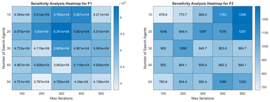
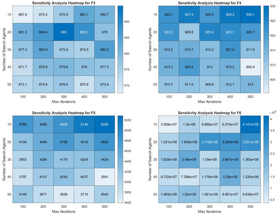
Figure 7.
Heatmap analysis over selected functions of CEC2022 (F1–F6).

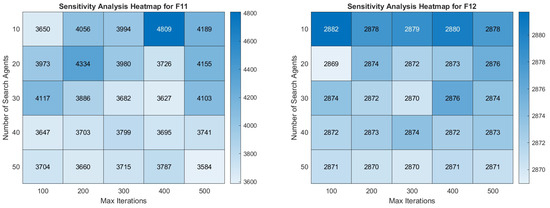
Figure 8.
Heatmap analysis over selected functions of CEC2022 (F7–F12).
5.8.4. Box Plot Analysis
The box plot analysis of COASaDE over the CEC2022 benchmark functions (F1–F12) (see Figure 9 and Figure 10) reveals valuable insights into the algorithm’s performance variability and robustness. Each box plot presents the distribution of the best fitness scores obtained across multiple runs, showcasing the median, quartiles, and potential outliers. For instance, the box plot for F10 displays a wide range of fitness scores with several outliers, indicating occasional deviations, likely due to the complex landscape of the function. In contrast, functions such as F8 and F9 exhibit more consistent performance with narrower interquartile ranges, suggesting a higher degree of reliability in these cases. The median values in these plots represent the central tendency of the algorithm’s performance, while the spread between the quartiles reflects the variability, with the presence of outliers highlighting instances where the algorithm significantly deviates from its typical performance.
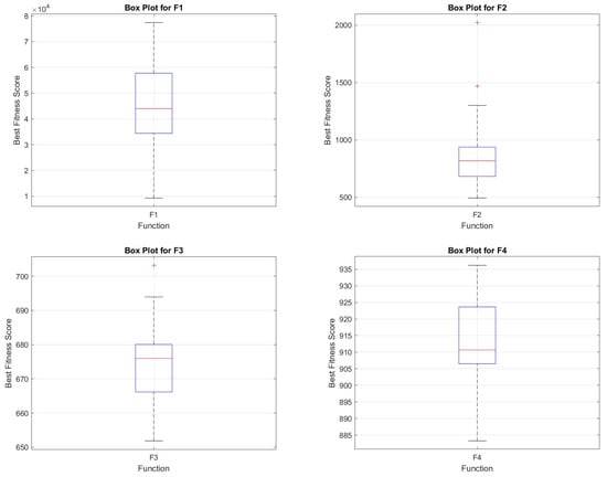
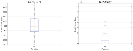
Figure 9.
Box plot analysis over selected functions of CEC2022 (F1–F6).
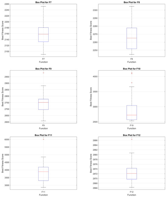
Figure 10.
Box plot analysis over selected functions of CEC2022 (F7–F12).
5.9. Histogram Analysis
The histograms provide a detailed view of the distribution of the final fitness values achieved by the COASaDE algorithm across various functions from the CEC2022 benchmark, as shown in Figure 11 and Figure 12. For F1, the histogram shows a spread with a peak around , indicating that the algorithm often converges to higher fitness values, with a few instances reaching up to . F2 exhibits a broad distribution, with a significant concentration of values between 600 and 1000 and some outliers extending beyond 1200. For F3 the histogram is more centered, with most values clustering around 670–680, indicating relatively consistent performance. The distribution for F4 shows a peak around 900–920, highlighting a narrower range of final fitness values. F5 has a more varied distribution, peaking around 3500–4500, suggesting a wide range of convergence results. For F6, the fitness values are mostly concentrated around lower values, with a significant drop-off as values increase, indicating that the algorithm often finds solutions with lower fitness values. F7 shows a more evenly spread distribution with a central tendency around 2100–2200. For F8 the distribution is highly skewed, with the majority of values around 2250 but with a few instances stretching up to 2400. F9 presents a relatively normal distribution centered around 2700–2800, indicating stable performance. Finally, the histogram for F10 is skewed, with a significant concentration of values around 2400–2800 and a long tail reaching up to 3800, suggesting occasional higher fitness values.

Figure 11.
Histogram analysis over selected functions of CEC2022 (F1–F6).
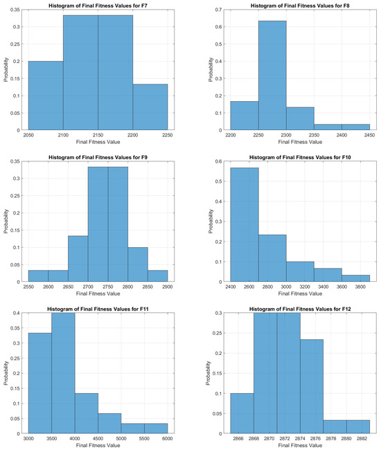
Figure 12.
Histogram analysis over selected functions of CEC2022 (F7–F12).
6. Application of COASaD for Solving Engineering Design Problems
6.1. Welded Beam Design Problem
The welded beam design problem represents a complex engineering optimization challenge aimed at identifying optimal beam dimensions that meet specific mechanical constraints while minimizing a cost function. The cost function associated with material and manufacturing expenses is provided by Equation (23):
where , , , and are the design variables.
The mechanical constraints are formulated based on fundamental principles of mechanical engineering, and are represented by the following Equations (24)–(26).
The constraint functions are defined in Equation (33).
To ensure adherence to these constraints during the optimization process, the penalty functions shown in Equation (34) are employed:
where v is a vector that flags each constraint’s violation, ensuring that the design meets mechanical requirements while optimizing cost.
Figure 13 illustrates a welded beam subjected to a point load P. It details dimensions such as the total length L, beam heights h and widths , and weld lengths and thickness values . These parameters are critical for assessing the beam’s structural integrity and performance under load.
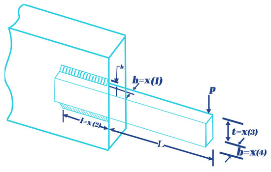
Figure 13.
Diagram of the welded beam.
The results achieved by COASaDE for the welded beam design problem (Table 13) demonstrate its superiority compared to several other optimization algorithms. COASaDE achieved the best objective function value (optimal) of 1.674E+00, outperforming all other optimizers in the study. It also maintained the lowest mean objective value (1.674E+00) and standard deviation (8.940E-04), indicating both accuracy and consistency in finding optimal solutions. When comparing COASaDE to other optimizers, notable differences can be observed. While COA had an optimal value of 1.670E+00, very close to that of COASaDE, its mean objective value was higher at 1.731E+00, with a standard deviation of 6.635E-02. This indicates that while COA occasionally found good solutions, it was less consistent than COASaDE. GWO had an optimal of 1.673E+00, also close to COASaDE, but with a higher mean of 1.733E+00 and a larger standard deviation of 1.089E-01, showing more variability in finding optimal solutions compared to COASaDE. AVOA had an optimal of 1.698E+00, with a mean of 1.792E+00 and a standard deviation of 1.422E-01, highlighting AVOA’s inconsistency. CSA achieved an optimal of 1.777E+00, with a mean of 1.793E+00 and a standard deviation of 1.366E-02, showing consistency but inferior overall performance. COOT had an optimal of 1.782E+00 with a mean of 1.838E+00 and a standard deviation of 4.840E-02, showing less accuracy and consistency. In terms of computational time, COASaDE performed efficiently with a recorded time of 0.379633, which was competitive with other algorithms such as GWO (0.375307) and AVOA (0.389991) and faster than others such as CSA (0.5748) and DBO (0.902343).
Table 13.
Welded beam design problem results.
6.2. Pressure Vessel Design Problem
The pressure vessel design problem is an optimization challenge that involves determining the optimal dimensions of a cylindrical vessel with hemispherical ends. The main objective is to minimize the material cost while ensuring that the structure meets specific structural and dimensional constraints. This task is pivotal in industries where pressure vessels are essential components, such as in chemical processing, power generation, and aerospace applications.
Objective function: The objective function is based on the physical and geometrical properties of the vessel. The function is structured to calculate the total material cost by considering the dimensions and material thickness of the vessel. The cost function is articulated in Equation (36):
The design variables for the vessel are defined with specific measurements in inches. The variable represents the thickness of the shell, corresponds to the thickness of the heads, is the inner radius of the vessel, and denotes the length of the cylindrical section of the vessel. Each of these variables is critical for specifying the structural dimensions and ensuring the integrity of the vessel’s design.
These variables (, , , and ) are crucial as they directly impact both the structural integrity and cost-efficiency of the vessel. The objective of the optimization problem is to determine the values of these variables that minimize the material cost while ensuring adherence to safety and performance standards.
The pressure vessel design problem focuses on determining the optimal dimensions of a cylindrical vessel with hemispherical ends to minimize the material cost while ensuring compliance with structural and dimensional constraints. The design challenge is depicted in Figure 14, which illustrates the vessel and its components.
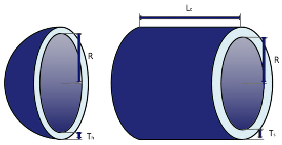
Figure 14.
Diagram of cylindrical vessel with hemispherical ends.
Objective Function:
The objective function aims to minimize the cost associated with the materials used in the construction of the pressure vessel. This objective is quantified in the cost function expressed in Equation (36):
where , , , and represent the thickness of the shell, the thickness of the heads, the inner radius, and the length of the cylindrical section, respectively.
Constraints:
The constraints are designed to ensure that the vessel’s dimensions are both feasible and meet all design requirements, and are detailed in Equations (37)–(44).
Constraints and relate the shell and head thickness to the radius, ensuring structural integrity. Constraint checks the internal volume against a prescribed limit. Constraints through are simple bounding constraints that restrict the size and dimensions of the vessel components.
Penalty function:
The optimization problem utilizes a penalty method in which each constraint violation contributes significantly to the objective function, effectively penalizing infeasible solutions, as shown in Equation (45):
where v is an indicator vector in which each element is set to 1 if the corresponding constraint is violated, helping to steer the optimization process towards feasible designs.
COASaDE achieves an optimal cost of , matched by several other high-performance algorithms such as SHIO, SCA, MGO, HOA, HLOA, FVIM, and EAO, demonstrating competitive results. Notably, COASaDE consistently reaches identical optimal design parameters (, , , ) to those reported by the aforementioned optimizers, indicating high precision in finding the global optimum. In contrast, algorithms such as SSA, POA, and COA exhibit higher optimal costs and significantly varied design parameters, reflecting less efficiency or stability in achieving designs with minimal cost. The consistent values across multiple dimensions by COASaDE and select others highlight the robustness and reliability of these algorithms in converging to an optimal solution, marking them as preferable choices for this specific engineering optimization task.
The results of COASaDE on the pressure vessel design problem (Table 14) highlight its effectiveness compared to other optimization algorithms. COASaDE achieved the optimal objective function value (optimal) of 5.885E+03, outperforming other optimizers with a mean of 6.091E+03 and a standard deviation of 4.492E+02. This indicates both high accuracy and consistency. In comparison, HHO also reached an optimal value of 5.885E+03, but with a higher mean (5.921E+03) and a smaller standard deviation (6.968E+01), showing good consistency but slightly lower overall performance. COA matched the optimal value of 5.885E+03 with an exceptionally low standard deviation (3.008E-02), highlighting remarkable consistency but a slightly lower mean (5.885E+03) than COASaDE. AO had an optimal value of 5.886E+03, with a mean of 5.902E+03 and a standard deviation of 1.841E+01, indicating good but less consistent performance. CSA achieved an optimal value of 5.889E+03, with a higher mean of 6.314E+03 and a standard deviation of 4.464E+02, showing less consistency and accuracy. AVOA obtained an optimal value of 5.901E+03, with a mean of 5.943E+03 and a standard deviation of 4.891E+01, demonstrating more variability. Other algorithms such as SA, ChOA, COOT, DBO, and SCA showed progressively higher optimal values and greater variability, with higher means and standard deviations, indicating less consistent and accurate performance.
Table 14.
Pressure vessel design problem results.
6.3. Spring Design Problem
The spring design problem is a prevalent optimization challenge in mechanical engineering. It involves determining the optimal dimensions of a coiled spring to minimize the material used in its construction while complying with specific mechanical and design constraints. The problem is typically expressed through the MATLAB function P3(x), which evaluates the performance and feasibility of different spring designs based on their dimensions.
Objective function:
The objective function is formulated to capture the total energy stored in the spring, which is directly affected by the physical dimensions of the spring. This function is strategically designed to minimize the material usage, potentially lowering production costs and enhancing material efficiency. The objective function is defined as Equation (46).
In this formulation, , , and represent the wire diameter, mean coil diameter, and number of active coils, respectively. These variables are crucial, as they significantly impact the mechanical properties of the spring, such as its stiffness and load-bearing capacity.
Constraints:
The design of the spring is subject to several constraints that are essential for ensuring both functionality and durability. These include stress constraints to prevent material failure, space constraints to ensure the spring fits within a predetermined design envelope, and resonance constraints to avoid vibrational issues that could arise in the operational environment. Each of these factors plays a critical role in the holistic design and successful application of the spring.
These constraints are typically represented as functions of the design variables , , and ; they ensure that the spring can perform its intended function safely and effectively. For instance, the stress within the spring must not exceed the yield strength of the material used.
Therefore, the optimization problem involves finding values for , , and that minimize the objective function while satisfying all imposed constraints. This problem is often solved using numerical methods that explore a range of potential designs to find the most efficient and practical solution.
The optimization of spring design involves determining the optimal dimensions of a coiled spring to ensure minimal material usage while adhering to the strict mechanical and design constraints.
Objective function:
The objective function is designed to minimize the material cost and potential energy stored during compression. This function is expressed in Equation (47):
where , , and are variables representing the wire diameter, mean coil diameter, and number of active coils, respectively. Each variable significantly contributes to the spring’s physical characteristics.
Constraints:
The design constraints atr crucial for maintaining the spring’s structural integrity and functionality, and are detailed in Equations (48) through (51).
These constraints ensure that the spring does not succumb to stresses, excessive deflections, or operational limitations. Specifically, constraints and address stress and deflection limits critical to the spring’s mechanical performance. Constraint sets a lower bound on the fundamental frequency, ensuring that the spring operates safely within its dynamic range. Additionally, constraint imposes a dimensional constraint, likely related to the installation space requirements, ensuring that the spring fits appropriately within its designated environment.
Penalty function:
To enforce these constraints effectively within the optimization process, a penalty function is used, as shown in Equation (52):
where v is an indicator vector in which each element is set to 1 if the corresponding constraint is violated, ensuring that noncompliant designs are discouraged and steering the optimization towards feasible and efficient solutions.
The results of COASaDE on the spring design problem (Table 15) highlight its superior performance compared to other optimization algorithms. COASaDE achieved the optimal objective function value (optimal) of 1.267E-02, consistently maintaining this value with a mean and standard deviation both at 1.267E-02 and 3.570E-08, respectively, indicating exceptional accuracy and consistency. In comparison, COA achieved the same optimal value of 1.267E-02 but with a slightly higher mean of 1.268E-02 and a standard deviation of 1.655E-05, showing slightly less consistency. SA matched the optimal value of 1.267E-02 with a mean of 1.269E-02 and a standard deviation of 4.403E-05, indicating good but less consistent performance. GWO also achieved the optimal value of 1.267E-02, with a mean of 1.269E-02 and a standard deviation of 4.496E-05, showing similar variability. CSA matched the optimal value of 1.267E-02 but with a higher mean of 1.314E-02 and a larger standard deviation of 6.621E-04, demonstrating less consistency and accuracy. COOT achieved the optimal value but had an anomalously high mean and standard deviation, indicating instability. Other algorithms, such as ChOA, WOA, HGS, AO, AVOA, DBO, SCA, and HHO, showed progressively higher optimal values and greater variability, indicating less consistent and accurate performance. The ranking in the table underscores COASaDE’s top performance, securing the first rank and highlighting its robustness, precision, and efficiency in solving the spring design optimization problem.
Table 15.
Spring design problem results.
6.4. Speed Reducer Design Problem
The speed reducer design problem is a complex optimization task centered around minimizing the cost function associated with the design of a gear train within a speed reducer. This problem encapsulates a myriad of mechanical design constraints, aiming to achieve an optimal balance between material cost, geometry, and structural limits. The objective is to design a speed reducer that is cost-effective, structurally sound, and operationally efficient.
Objective function:
The objective function for the speed reducer design problem incorporates various geometric and material cost factors, reflecting the complex interdependencies of the gear train components. The function is formulated as shown in Equation (53).
This equation captures the essential cost elements and mechanical requirements integral to designing an efficient speed reducer.
This function is meticulously crafted to account for various factors. Primarily, it addresses the costs associated with the material used in the gear train, which is significantly influenced by dimensions such as face width (), gear tooth thickness (), and gear diameters (, , ). Additionally, the function considers the structural integrity and operational efficacy, which are modulated by variables and . These variables represent the gear diameters, and are crucial for ensuring the gear’s mechanical performance.
The careful selection of these terms ensures that the function reflects the trade-offs between material strength, weight, and overall cost of the speed reducer. The objective needs to not just minimize the cost but also ensure that the speed reducer meets all operational and safety standards.
Constraints:
The design of the speed reducer must also adhere to a series of constraints which ensure that the product is not only economically viable but also meets all required performance criteria. These constraints include but are not limited to stress and strain limits, dimensional tolerances, and compatibility requirements for interfacing with other mechanical systems. Each constraint is typically formulated as a function of the design variables, and is critical in guiding the optimization process towards feasible solutions.
The speed reducer design problem is a critical engineering optimization challenge aimed at minimizing a cost function associated with the gear train design within a speed reducer. The objective is to balance material costs, geometric considerations, and structural limits. Figure 15 illustrates the complex interplay of these factors.

Figure 15.
Design of the speed reducer gear train.
Objective function:
The objective function integrates the material costs and geometric dependencies of various components, as expressed in Equation (54).
This function is designed to minimize the material cost while considering the weight and durability of the speed reducer’s components.
Constraints:
The design constraints, which are essential for ensuring the design’s feasibility and efficiency, are formulated as shown below and illustrated in Figure 15.
These constraints ensure that the speed reducer can withstand bending stresses, maintain surface durability, resist stress concentration, and fit geometrically within the overall design.
Penalty function
To ensure compliance with these constraints, a penalty function is employed, as shown in Equation (66):
where v is an indicator vector that flags each constraint violation to ensure that designs not meeting the safety and performance standards are penalized, thereby guiding the optimization process towards feasible solutions.
Table 16 shows that COASaDE achieved the best score (Best Score) of 2.994E+03, maintaining a low mean score of 2.998E+03 and a standard deviation of 1.242E+01 on the speed reducer design problem. In comparison, COA achieved the same best score of 2.994E+03 with an exceptionally low standard deviation of 1.104E-12, demonstrating remarkable consistency, although its recorded time was significantly higher at 2.472202. ChOA matched the best score of 2.994E+03 but with a higher mean of 3.000E+03 and a standard deviation of 9.610E+00, showing slightly more variability. CSA also achieved the best score of 2.994E+03 with a minimal standard deviation of 1.696E-08 and a slightly higher mean, indicating very consistent performance. AO matched the best score but had a higher mean and standard deviation, reflecting less precision. Other algorithms such as WOA, SA, AVOA, HGS, DBO, COOT, GWO, and HHO showed progressively higher best scores and greater variability, indicating less consistent and accurate performance.
Table 16.
Speed reducer design problem results.
6.5. Cantiliver Design Problem
The cantilever design problem is an engineering challenge that involves optimizing the dimensions of a cantilever structure. The goal is to minimize the material cost while ensuring structural stability under various loading conditions. This optimization problem is critical in fields such as civil engineering, aerospace, and mechanical systems, where cantilevers are frequently used components.
Objective function:
The objective function is specifically designed to represent the total material cost associated with the construction of the cantilever. This function is quantitatively formulated as shown in Equation (67).
In this model, , , , , and correspond to the dimensions of the cantilever, such as the thickness or length of different segments. Each variable contributes linearly to the material cost, indicating that any changes in these dimensions will have a direct impact on the overall cost of the structure.
Constraints:
To ensure the structural stability of the cantilever under various loads, several critical constraints must be considered. These include stress constraints designed to prevent material failure under maximum expected loads, deflection constraints aimed at ensuring the cantilever does not deform excessively under load, and natural frequency constraints intended to avoid resonant frequencies that could lead to structural failure. Each of these constraints plays a vital role in the design and safety assurance of the cantilever structure.
These constraints are generally formulated as functions of the design variables, ensuring that the cantilever remains both economical and safe under operational conditions.
Therefore, the design problem involves not only minimizing the objective function but also satisfying a series of structural and performance-based constraints. This holistic approach ensures the creation of a cantilever that is both cost effective and robust in its application.
The cantilever design problem (see Figure 16) is a critical challenge in structural engineering, where the goal is to optimize the dimensions of a cantilever to minimize material costs while ensuring that the structure can withstand operational loads without failure. The optimization is particularly focused on balancing cost efficiency with the structural integrity required to handle expected stresses and deflections.

Figure 16.
Cantilever design problem.
Objective function:
The objective function is calculated to determine the total cost of materials used in the construction of the cantilever based on the dimensions of its various segments, as shown in Equation (68):
where , , , , and might correspond to the thicknesses or lengths of different segments of the cantilever, where each variable affects the material cost linearly.
Constraints:
The cantilever must meet specific structural stiffness and strength criteria, which are formulated in constraint shown in the following Equation (69).
This constraint is derived from the bending stiffness or strength requirements, where the terms reflect the inverse cube relationship between dimension (likely thickness) and bending stiffness or strength for each segment, thereby ensuring the cantilever’s adequacy in terms of stiffness and strength.
Penalty function:
To enforce the structural requirements and discourage noncompliance, the penalty function detailed in Equation (70) is utilized.
In this function, v is an indicator vector in which each element is set to 1 if the corresponding constraint is violated. This setup imposes a high cost on designs that do not meet the structural criteria, thereby promoting compliance with the required standards.
As can be seen in Table 17, COASaDE achieved an optimal objective function value (optimal) of 1.340E+00, consistently maintaining this value with a mean of 1.340E+00 and a standard deviation of 2.171E-05, indicating exceptional accuracy and consistency. In comparison, CSA achieved the same optimal value of 1.340E+00 with a slightly higher standard deviation of 1.005E-04, demonstrating good consistency but slightly less precision. GWO also matched the optimal value with a standard deviation of 8.980E-05, showing comparable performance to CSA. COA achieved the optimal value with a mean of 1.340E+00 and a higher standard deviation of 3.502E-04, reflecting more variability. HGS and DBO both matched the optimal value but showed higher means and standard deviations, indicating less consistent performance. Other algorithms such as COOT, HHO, AVOA, AO, SA, ChOA, BWO, SCA, and WOA demonstrated progressively higher optimal values, means, and standard deviations, indicating less consistent and accurate performance.
Table 17.
Cantiliver design problem results.
6.6. I-Beam Design Problem
The I-beam design problem involves optimizing the geometry of an I-beam to achieve minimal deflection under a specific load while ensuring that the beam’s cross-sectional area meets certain size requirements. This problem exemplifies the essential balance between efficient material use and optimal structural performance in beam design.
Objective function:
The objective function is formulated to minimize the beam’s deflection by maximizing the section modulus, which is a measure of the beam’s resistance to bending. This is mathematically represented by the inverse of the section modulus, as shown in Equation (71):
where b represents the width of the beam, h is the overall height, is the web thickness, and is the flange thickness. The objective is to minimize z, thereby reducing the deflection under load.
Constraint:
As illustrated in Figure 17, the design includes a constraint to ensure that the total material used for the beam does not fall below a specific threshold, which is important for maintaining structural integrity and compliance with industry standards. The constraint is formulated in the following Equation (72).

Figure 17.
Schematic of the optimized I-beam geometry [41].
This constraint is interpreted as ensuring a minimum cross-sectional area or weight of the beam, which is necessary to meet safety regulations and structural requirements.
Penalty function:
To enforce compliance with this constraint, a penalty function is employed, as detailed in Equation (73):
where v is an indicator vector in which each element is set to 1 if the corresponding constraint is violated. This approach ensures that designs not meeting the required standards incur a significant cost, thereby steering the optimization process towards feasible and compliant designs.
As can be seen in Table 18, COASaDE achieved the best score of 6.626E-03, consistently maintaining this value with an incredibly low standard deviation of 1.042E-18, indicating exceptional accuracy and consistency. COA matched this best score with an equally low standard deviation of 9.143E-19, demonstrating remarkable consistency. CSA, ChOA, and SCA also matched the best scores with similarly low standard deviations, reflecting their consistency in performance. DBO achieved the same best score with a slightly higher standard deviation of 6.176E-09, showing minor variability. WOA, AO, AVOA, SA, HGS, and COOT all matched the best scores with low standard deviations, although slightly higher than those of COA and CSA, indicating good consistency but slightly less precision.
Table 18.
I-beam design problem results.
Furthermore, COASaDE successfully achieved the optimal value of , precisely matching the optimal design variables (, , , ) identified by the vast majority of other optimizers, including WSO, SSA, SHIO, SCA, and EAO, which demonstrates consensus on the solution’s accuracy and effectiveness across different algorithms. This uniformity in achieving optimal values and design variables highlights the robustness and reliability of these algorithms in precisely solving structural design optimizations under defined constraints. Interestingly, all algorithms, including MPA, exhibited close results with almost negligible variations, indicating that these optimization techniques are well suited for engineering applications where precision is crucial. Notably, COASaDE stands out with a perfect standard deviation of , suggesting its superior ability to consistently reach the exact optimal solution on every run, setting a benchmark in solution consistency among its peers.
6.7. Three-Bar Design Problem
The three-bar truss design problem is a classic engineering optimization challenge that focuses on finding the optimal dimensions of a truss structure. The objective is to minimize the cost of the structure while ensuring that it performs adequately under specified load constraints, embodying a balance between economic efficiency and structural integrity.
Objective function:
The objective function for this problem calculates the cost associated with the truss, where the dimensions directly influence material usage and consequently the overall cost. This relationship is formalized in the following Equation (74):
where and represent the cross-sectional areas of the truss members. This formula incorporates coefficients that likely reflect the cost per unit length of the materials used adjusted for the truss’s specific geometric configuration.
Constraints:
The design must meet several constraints in order to ensure that the stress in each member remains within safe limits, as detailed in Equations (75)–(77).
These constraints are derived from the stress distribution formulas in the truss members, ensuring that the stress does not exceed the material’s yield strength. Each constraint addresses different loading conditions and geometric relationships in the truss design, which is crucial for maintaining safety and functionality.
Penalty function:
To ensure compliance with these constraints, the penalty functions shown in Equation (78) is employed.
In this function, v is an indicator vector in which each element is set to 1 if the corresponding constraint is violated. This setup imposes a significant cost on noncompliant designs, effectively steering the optimization algorithm towards solutions that satisfy all performance criteria, thereby ensuring both safety and cost efficiency.
As can be seen in Table 19, COASaDE achieved the minimum value of 2.639E+02, consistently maintaining this value with a mean of 2.639E+02 and an incredibly low standard deviation of 8.994E-12, indicating exceptional accuracy and consistency. CSA matched the optimal value of 2.639E+02 with a slightly higher standard deviation of 1.067E-10, demonstrating very good consistency. GWO also matched the optimal value but had a higher standard deviation of 8.707E-04, indicating more variability. COA achieved the optimal value with a higher standard deviation of 4.776E-03, reflecting more variability. GOA and COOT both matched the optimal value but with even higher standard deviations of 8.400E-03 and 9.651E-03, respectively, showing less precision. Other algorithms such as AVOA, HHO, DBO, ChOA, SCA, BO, SA, BWO, and WOA demonstrated progressively higher optimal values, means, and standard deviations, indicating less consistent and accurate performance. The ranking in the table reinforces COASaDE’s top performance, securing the first rank and highlighting its robustness, precision, and efficiency in solving the three-bar design optimization problem.
Table 19.
Three-bar design problem results.
7. Conclusions
In this paper, we have presented the Hybrid COASaDE Optimizer, a novel combination of the Crayfish Optimization Algorithm (COA) and Self-adaptive Differential Evolution (SaDE) designed to address complex optimization challenges and solve engineering design problems. The proposed hybrid approach leverages COA’s efficient exploration mechanisms, inspired by crayfish behavior, and SaDE’s adaptive exploitation capabilities, characterized by its dynamic parameter adjustment. This synergy aims to balance the exploration and exploitation phases to enhance the algorithm’s ability to effectively navigate diverse optimization landscapes. We have detailed the mathematical model of the Hybrid COASaDE algorithm, including the initialization and parameter setting, position update mechanisms, and integration of the mutation and crossover strategies from SaDE. The exploration phase utilizes COA’s behavior-based strategy to avoid premature convergence, while the exploitation phase employs SaDE’s adaptive techniques to refine the candidate solutions. Experimental evaluations were conducted using the CEC2022 and CEC2017 benchmark functions, demonstrating Hybrid COASaDE’s superior performance compared to both traditional and state-of-the-art optimization algorithms. The results were analyzed through various methods, including convergence curves, search history plots, sensitivity analysis, and statistical analyses such as box plots and histograms. These analyses confirm the robustness and efficiency of Hybrid COASaDE in finding optimal solutions. Furthermore, the applicability of Hybrid COASaDE was validated through several engineering design problems, including the welded beam, pressure vessel, spring, speed reducer, cantilever, I-beam, and three-bar truss design problems. Hybrid COASaDE consistently outperformed the other optimizers on each design problem while achieving the optimal solution.
Author Contributions
Conceptualization, H.N.F., A.I. and S.N.M.; methodology, H.N.F., A.I. and S.N.M.; software, H.N.F., A.I. and S.N.M.; validation, M.A.A.-B. and M.A.; formal analysis, H.N.F., M.A.A.-B. and M.A.; investigation, H.N.F., M.A.A.-B. and M.A.; writing—original draft preparation, H.N.F., A.I., S.N.M., M.A.A.-B. and M.A.; writing—review and editing, H.N.F., A.I., S.N.M. and M.A.A.-B.; visualization, H.N.F. and S.N.M.; supervision, H.N.F. and S.N.M.; project administration, H.N.F.; funding acquisition, M.A.A.-B. All authors have read and agreed to the published version of the manuscript.
Funding
This research was funded by Ajman University.
Data Availability Statement
The original data presented in the study are openly available in the paper.
Conflicts of Interest
The authors declare no conflict of interest.
References
- Abdel-Basset, M.; Abdel-Fatah, L.; Sangaiah, A.K. Metaheuristic algorithms: A comprehensive review. In Computational Intelligence for Multimedia Big Data on the Cloud with Engineering Applications; Academic Press: Cambridge, MA, USA, 2018; pp. 185–231. [Google Scholar]
- Kochenderfer, M.J.; Wheeler, T.A. Algorithms for Optimization; MIT Press: Cambridge, MA, USA, 2019. [Google Scholar]
- Diwekar, U.M. Introduction to Applied Optimization; Springer Nature: Berlin/Heidelberg, Germany, 2020; Volume 22. [Google Scholar]
- Blei, D.M.; Ng, A.Y.; Jordan, M.I. Latent dirichlet allocation. J. Mach. Learn. Res. 2003, 3, 993–1022. [Google Scholar]
- Fakhouri, H.N.; Alawadi, S.; Awaysheh, F.M.; Hamad, F. Novel hybrid success history intelligent optimizer with gaussian transformation: Application in CNN hyperparameter tuning. Clust. Comput. 2023, 27, 3717–3739. [Google Scholar] [CrossRef]
- Li, Q.; Tai, C.; Weinan, E. Stochastic modified equations and dynamics of stochastic gradient algorithms i: Mathematical foundations. J. Mach. Learn. Res. 2019, 20, 1474–1520. [Google Scholar]
- Gill, P.E.; Murray, W.; Wright, M.H. Practical Optimization; SIAM: Philadelphia, PA, USA, 2019. [Google Scholar]
- Yin, Z.Y.; Jin, Y.F.; Shen, J.S.; Hicher, P.Y. Optimization techniques for identifying soil parameters in geotechnical engineering: Comparative study and enhancement. Int. J. Numer. Anal. Methods Geomech. 2018, 42, 70–94. [Google Scholar] [CrossRef]
- Guo, K.; Yang, Z.; Yu, C.H.; Buehler, M.J. Artificial intelligence and machine learning in design of mechanical materials. Mater. Horizons 2021, 8, 1153–1172. [Google Scholar] [CrossRef] [PubMed]
- Fakhouri, S.N.; Hudaib, A.; Fakhouri, H.N. Enhanced optimizer algorithm and its application to software testing. J. Exp. Theor. Artif. Intell. 2020, 32, 885–907. [Google Scholar] [CrossRef]
- Shukri, S.E.; Al-Sayyed, R.; Hudaib, A.; Mirjalili, S. Enhanced multi-verse optimizer for task scheduling in cloud computing environments. Expert Syst. Appl. 2021, 168, 114230. [Google Scholar] [CrossRef]
- Hudaib, A.A.; Fakhouri, H.N. Supernova optimizer: A novel natural inspired meta-heuristic. Mod. Appl. Sci. 2018, 12, 32–50. [Google Scholar] [CrossRef]
- Fakhouri, H.N.; Alawadi, S.; Awaysheh, F.M.; Hani, I.B.; Alkhalaileh, M.; Hamad, F. A comprehensive study on the role of machine learning in 5G security: Challenges, technologies, and solutions. Electronics 2023, 12, 4604. [Google Scholar] [CrossRef]
- Zhan, Z.H.; Shi, L.; Tan, K.C.; Zhang, J. A survey on evolutionary computation for complex continuous optimization. Artif. Intell. Rev. 2022, 55, 59–110. [Google Scholar] [CrossRef]
- Ahvanooey, M.T.; Li, Q.; Wu, M.; Wang, S. A survey of genetic programming and its applications. KSII Trans. Internet Inf. Syst. (TIIS) 2019, 13, 1765–1794. [Google Scholar]
- Žilinskas, A.; Calvin, J. Bi-objective decision making in global optimization based on statistical models. J. Glob. Optim. 2019, 74, 599–609. [Google Scholar] [CrossRef]
- Fakhouri, H.N.; Hudaib, A.; Sleit, A. Hybrid particle swarm optimization with sine cosine algorithm and nelder–mead simplex for solving engineering design problems. Arab. J. Sci. Eng. 2020, 45, 3091–3109. [Google Scholar] [CrossRef]
- Lan, G. First-Order and Stochastic Optimization Methods for Machine Learning; Springer: Berlin/Heidelberg, Germany, 2020; Volume 1. [Google Scholar]
- Diakonikolas, I.; Kamath, G.; Kane, D.; Li, J.; Steinhardt, J.; Stewart, A. Sever: A robust meta-algorithm for stochastic optimization. In Proceedings of the International Conference on Machine Learning, Long Beach, CA, USA, 9–15 June 2019; pp. 1596–1606. [Google Scholar]
- Fakhouri, H.N.; Hudaib, A.; Sleit, A. Multivector particle swarm optimization algorithm. Soft Comput. 2020, 24, 11695–11713. [Google Scholar] [CrossRef]
- Erol, O.K.; Eksin, I. A new optimization method: Big bang–big crunch. Adv. Eng. Softw. 2006, 37, 106–111. [Google Scholar] [CrossRef]
- Powell, W.B. A unified framework for stochastic optimization. Eur. J. Oper. Res. 2019, 275, 795–821. [Google Scholar] [CrossRef]
- Bitar, R.; Wootters, M.; El Rouayheb, S. Stochastic gradient coding for straggler mitigation in distributed learning. IEEE J. Sel. Areas Inf. Theory 2020, 1, 277–291. [Google Scholar] [CrossRef]
- Mathew, T.V. Genetic Algorithm. 2012. Available online: https://datajobs.com/data-science-repo/Genetic-Algorithm-Guide-[Tom-Mathew].pdf (accessed on 9 June 2024).
- Zedadra, O.; Guerrieri, A.; Jouandeau, N.; Spezzano, G.; Seridi, H.; Fortino, G. Swarm intelligence-based algorithms within IoT-based systems: A review. J. Parallel Distrib. Comput. 2018, 122, 173–187. [Google Scholar] [CrossRef]
- Dorigo, M.; Stützle, T. Ant Colony Optimization: Overview and Recent Advances; Springer: Berlin/Heidelberg, Germany, 2019. [Google Scholar]
- Fakhouri, H.N.; Awaysheh, F.M.; Alawadi, S.; Alkhalaileh, M.; Hamad, F. Four vector intelligent metaheuristic for data optimization. Computing 2024, 106, 2321–2359. [Google Scholar] [CrossRef]
- Yang, X.S. Nature-Inspired Optimization Algorithms; Academic Press: Cambridge, MA, USA, 2020. [Google Scholar]
- Deng, W.; Xu, J.; Gao, X.Z.; Zhao, H. An enhanced MSIQDE algorithm with novel multiple strategies for global optimization problems. IEEE Trans. Syst. Man Cybern. Syst. 2020, 52, 1578–1587. [Google Scholar] [CrossRef]
- Seyyedabbasi, A. WOASCALF: A new hybrid whale optimization algorithm based on sine cosine algorithm and levy flight to solve global optimization problems. Adv. Eng. Softw. 2022, 173, 103272. [Google Scholar] [CrossRef]
- Ashraf, A.; Almazroi, A.A.; Bangyal, W.H.; Alqarni, M.A. Particle Swarm Optimization with New Initializing Technique to Solve Global Optimization Problems. Intell. Autom. Soft Comput. 2022, 31, 191. [Google Scholar] [CrossRef]
- Che, Y.; He, D. A hybrid whale optimization with seagull algorithm for global optimization problems. Math. Probl. Eng. 2021, 2021, 6639671. [Google Scholar] [CrossRef]
- Braik, M.; Al-Zoubi, H.; Ryalat, M.; Sheta, A.; Alzubi, O. Memory based hybrid crow search algorithm for solving numerical and constrained global optimization problems. Artif. Intell. Rev. 2023, 56, 27–99. [Google Scholar] [CrossRef]
- Wang, Z.; Luo, Q.; Zhou, Y. Hybrid metaheuristic algorithm using butterfly and flower pollination base on mutualism mechanism for global optimization problems. Eng. Comput. 2021, 37, 3665–3698. [Google Scholar] [CrossRef]
- Jia, H.; Zhou, X.; Zhang, J.; Abualigah, L.; Yildiz, A.R.; Hussien, A.G. Modified crayfish optimization algorithm for solving multiple engineering application problems. Artif. Intell. Rev. 2024, 57, 127. [Google Scholar] [CrossRef]
- Daulat, H.; Varma, T.; Chauhan, K. Augmenting the Crayfish Optimization with Gaussian Distribution Parameter for Improved Optimization Efficiency. In Proceedings of the 2024 International Conference on Cognitive Robotics and Intelligent Systems (ICC-ROBINS), Tamil Nadu, India, 17–19 April 2024; pp. 462–470. [Google Scholar]
- Jia, H.; Rao, H.; Wen, C.; Mirjalili, S. Crayfish optimization algorithm. Artif. Intell. Rev. 2023, 56, 1919–1979. [Google Scholar] [CrossRef]
- Qin, A.K.; Suganthan, P.N. Self-adaptive differential evolution algorithm for numerical optimization. In Proceedings of the 2005 IEEE Congress on Evolutionary Computation, Scotland, UK, 2–5 September 2005; Volume 2, pp. 1785–1791. [Google Scholar]
- Eltaeib, T.; Mahmood, A. Differential evolution: A survey and analysis. Appl. Sci. 2018, 8, 1945. [Google Scholar] [CrossRef]
- Pepelyshev, A.; Zhigljavsky, A.; Žilinskas, A. Performance of global random search algorithms for large dimensions. J. Glob. Optim. 2018, 71, 57–71. [Google Scholar]
- Ye, P.; Pan, G. Selecting the best quantity and variety of surrogates for an ensemble model. Mathematics 2020, 8, 1721. [Google Scholar] [CrossRef]
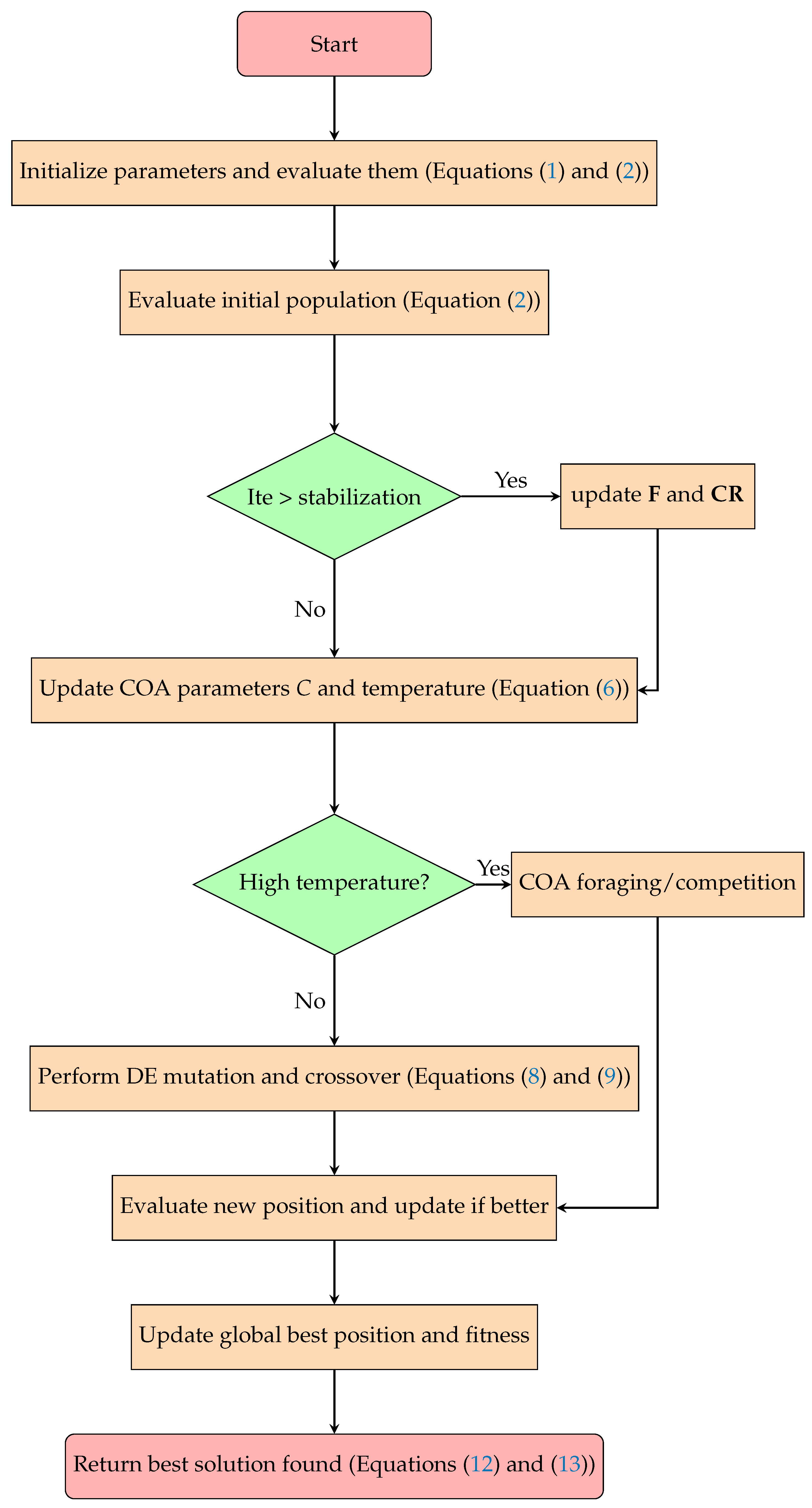

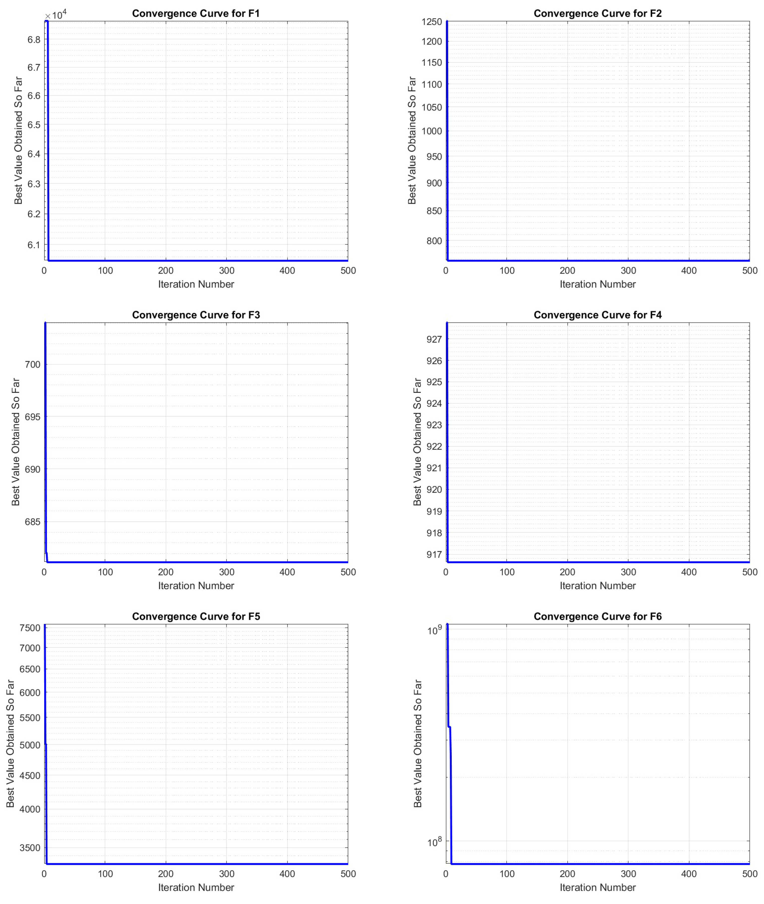
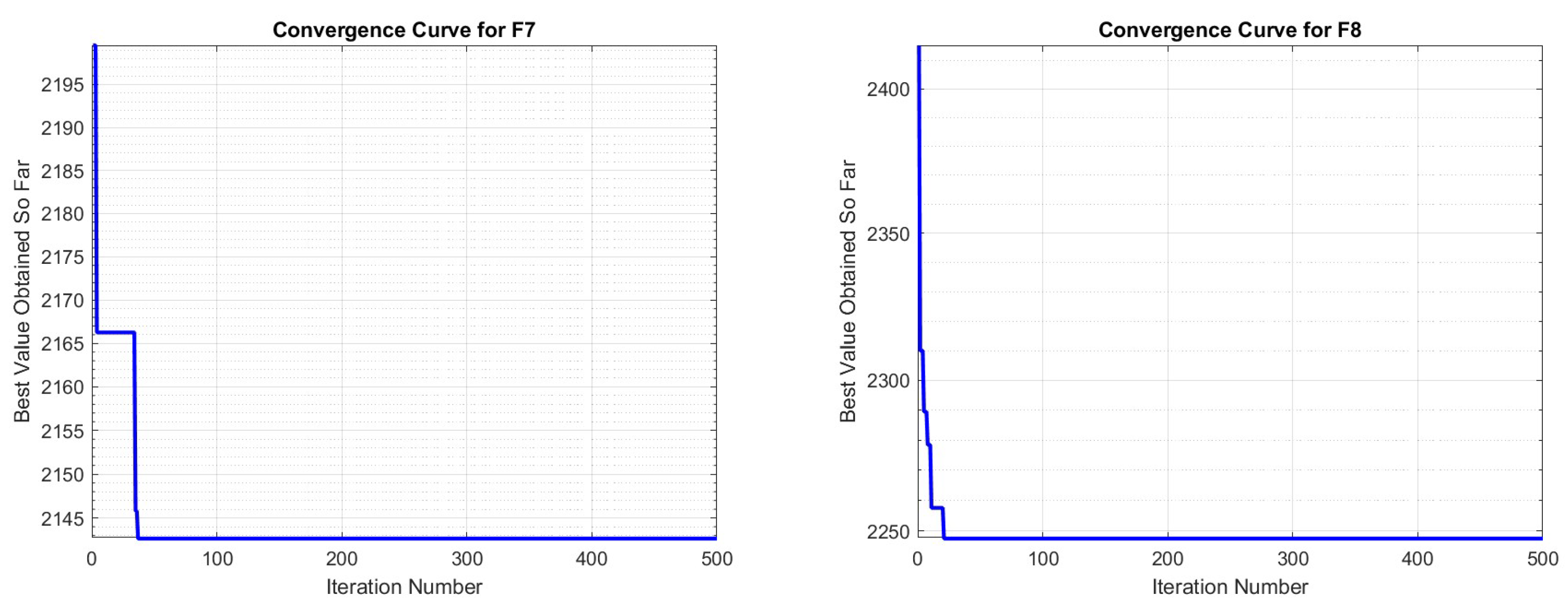
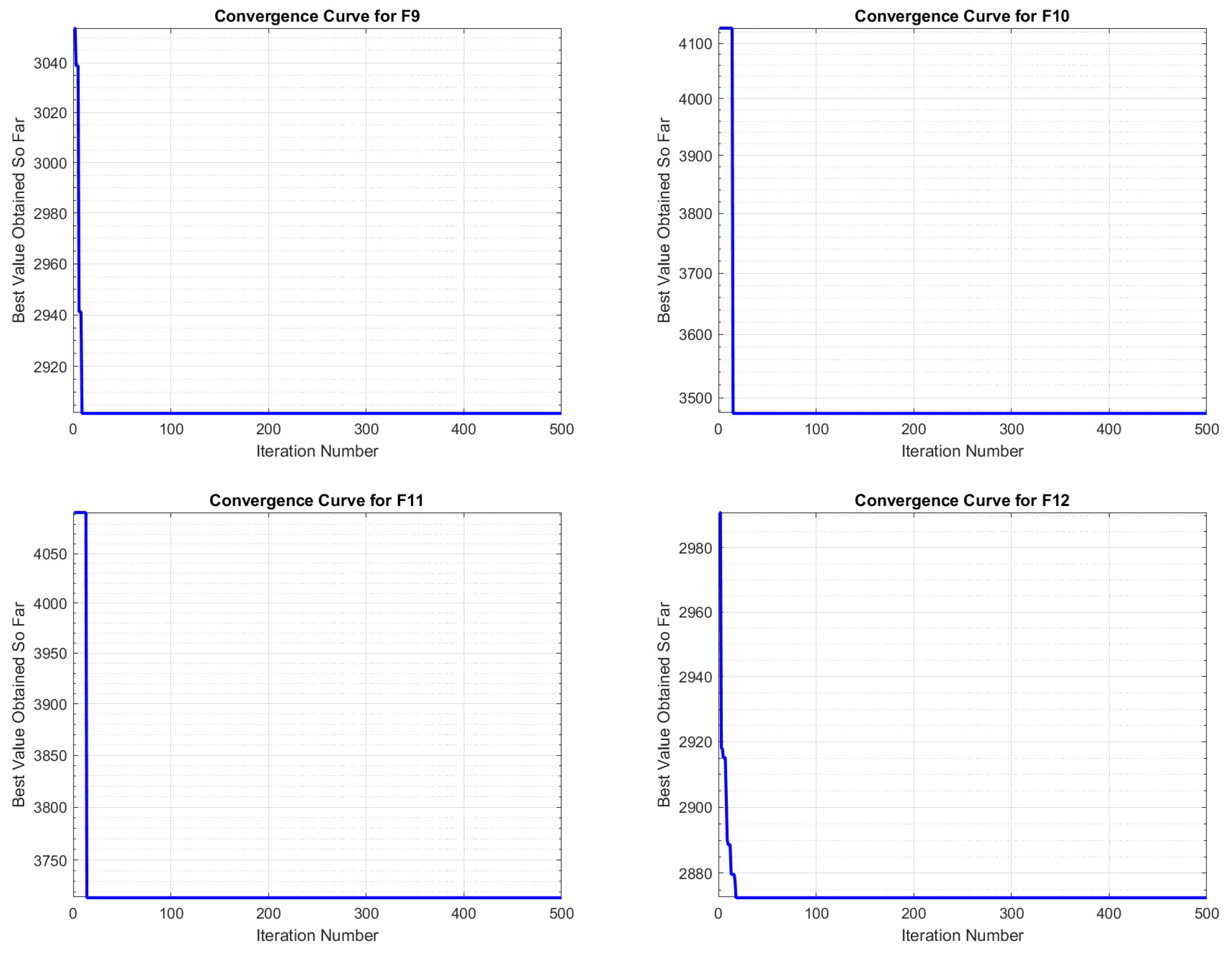
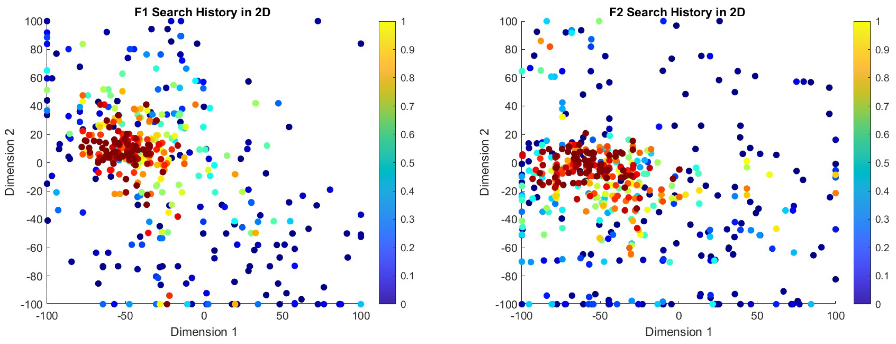
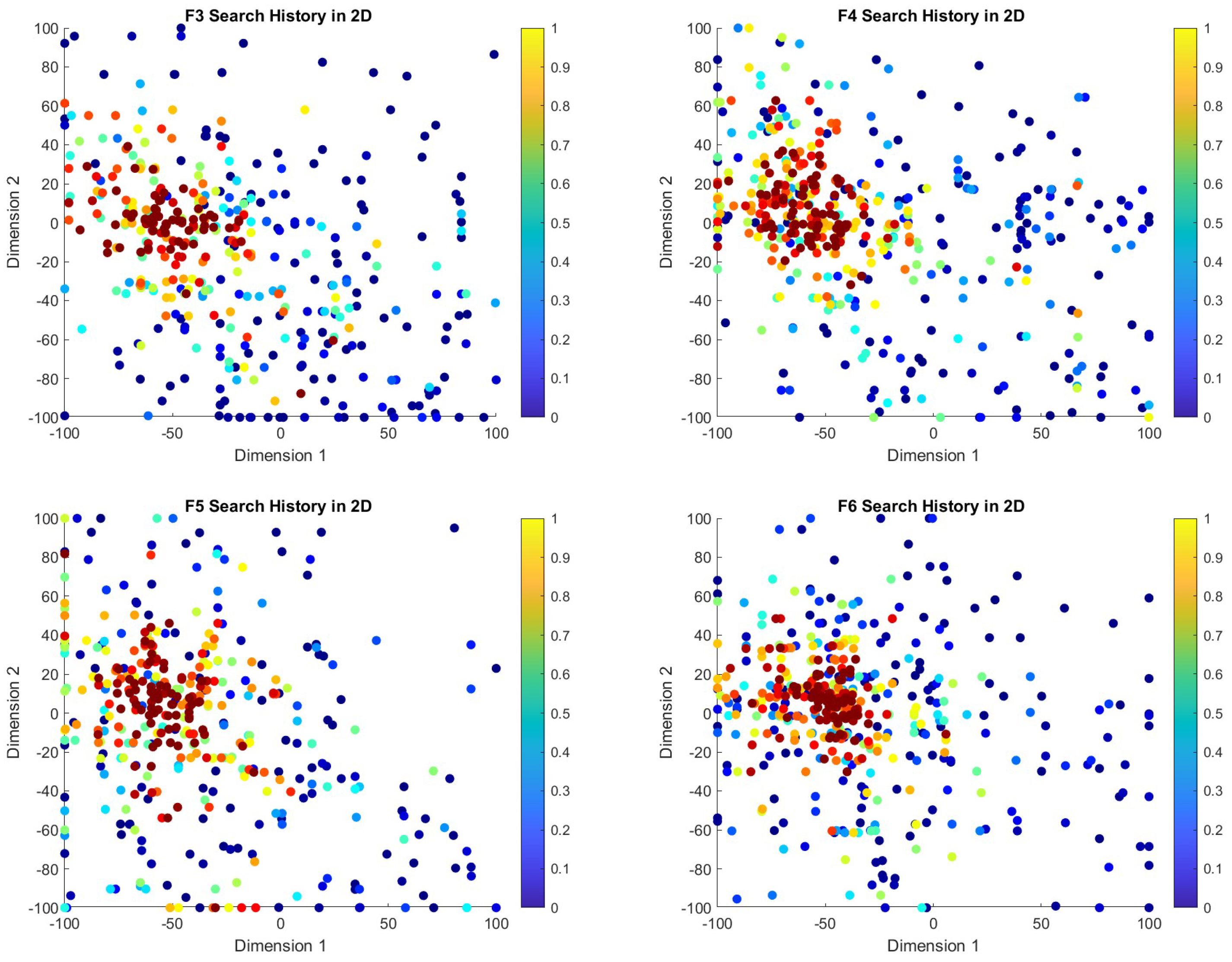
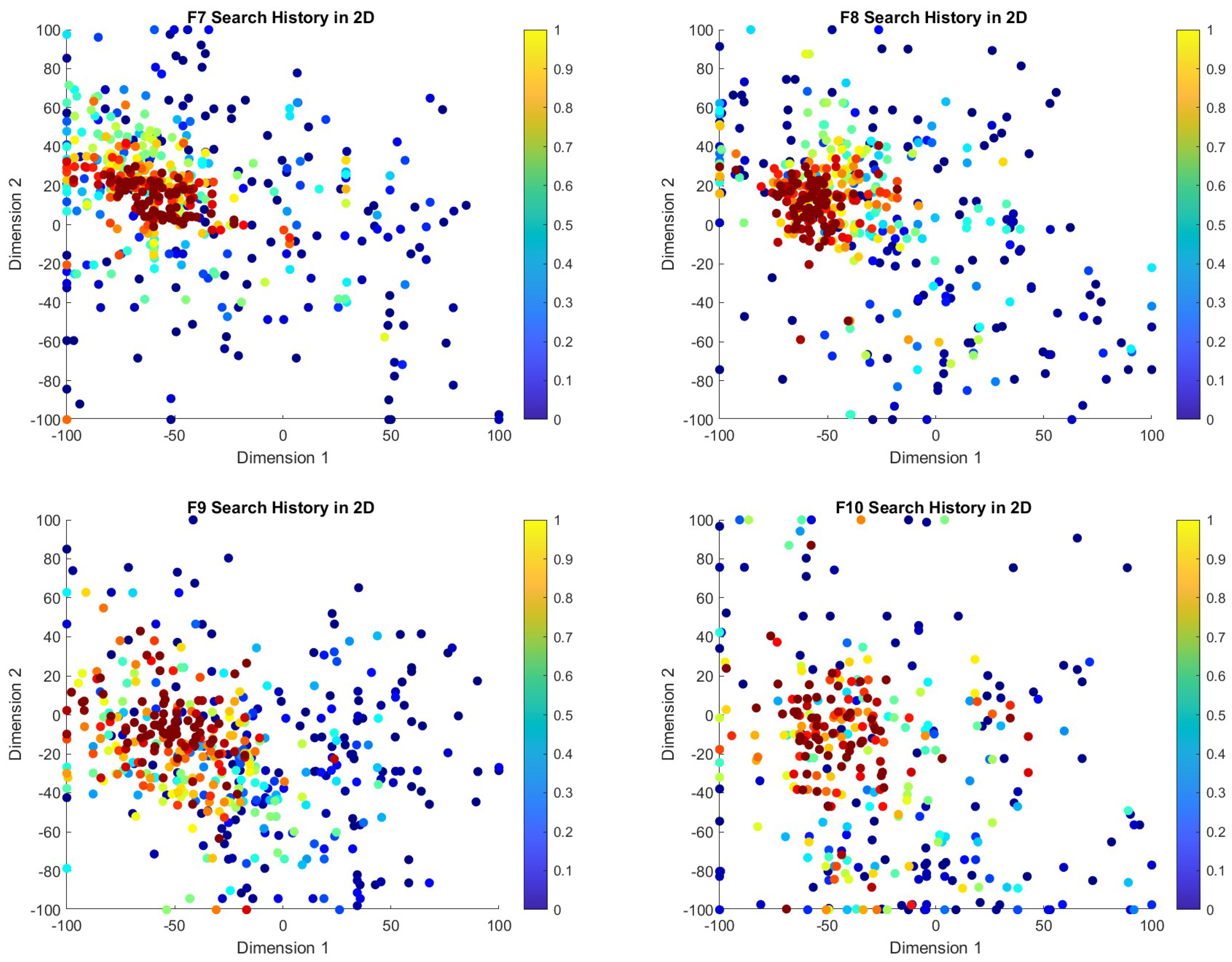
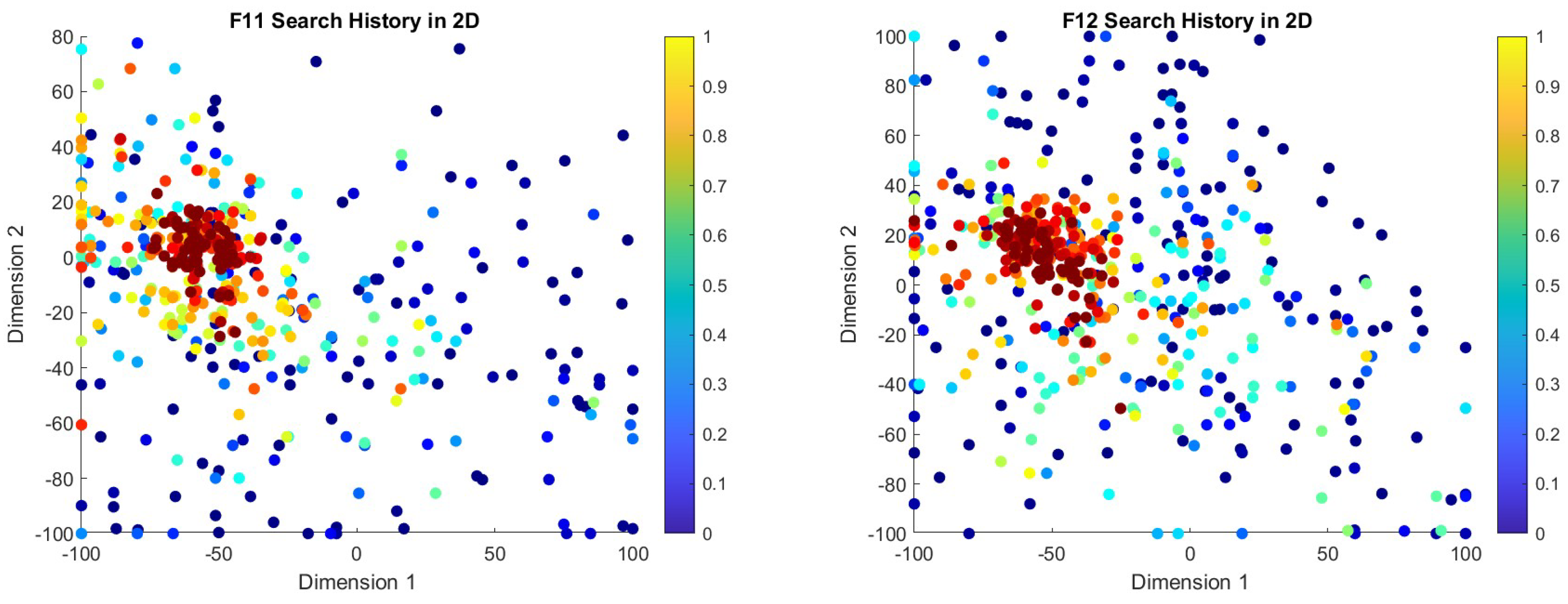
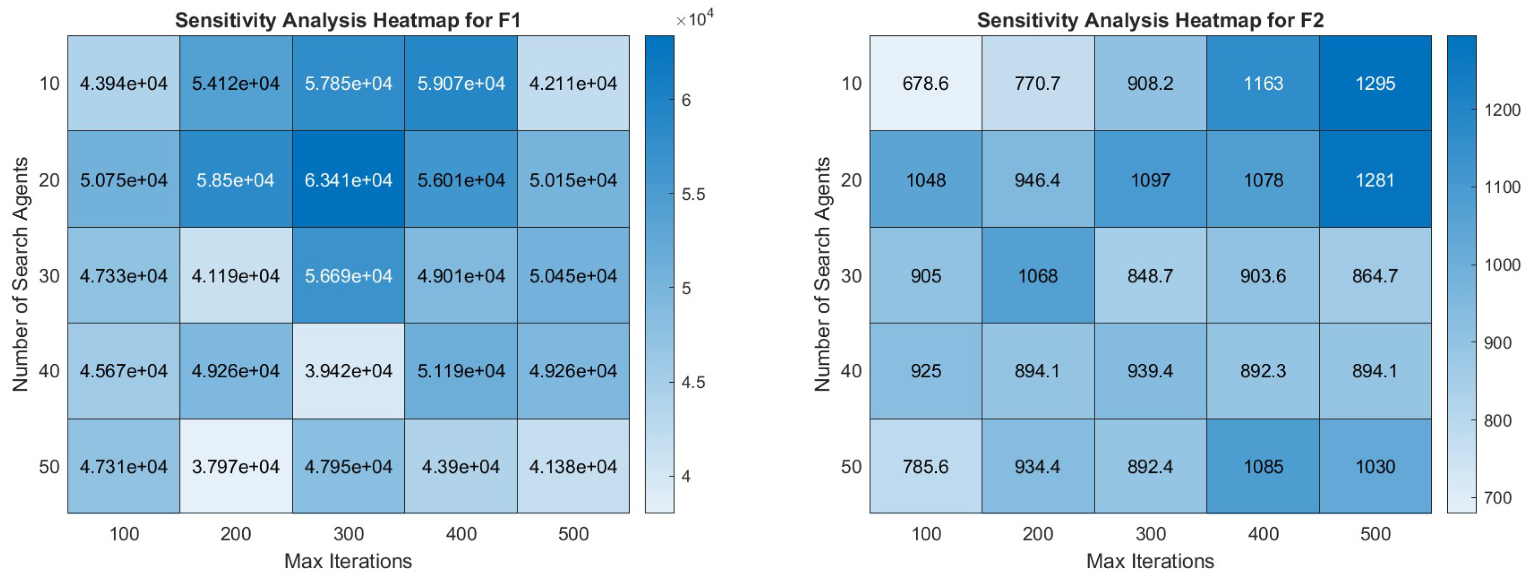
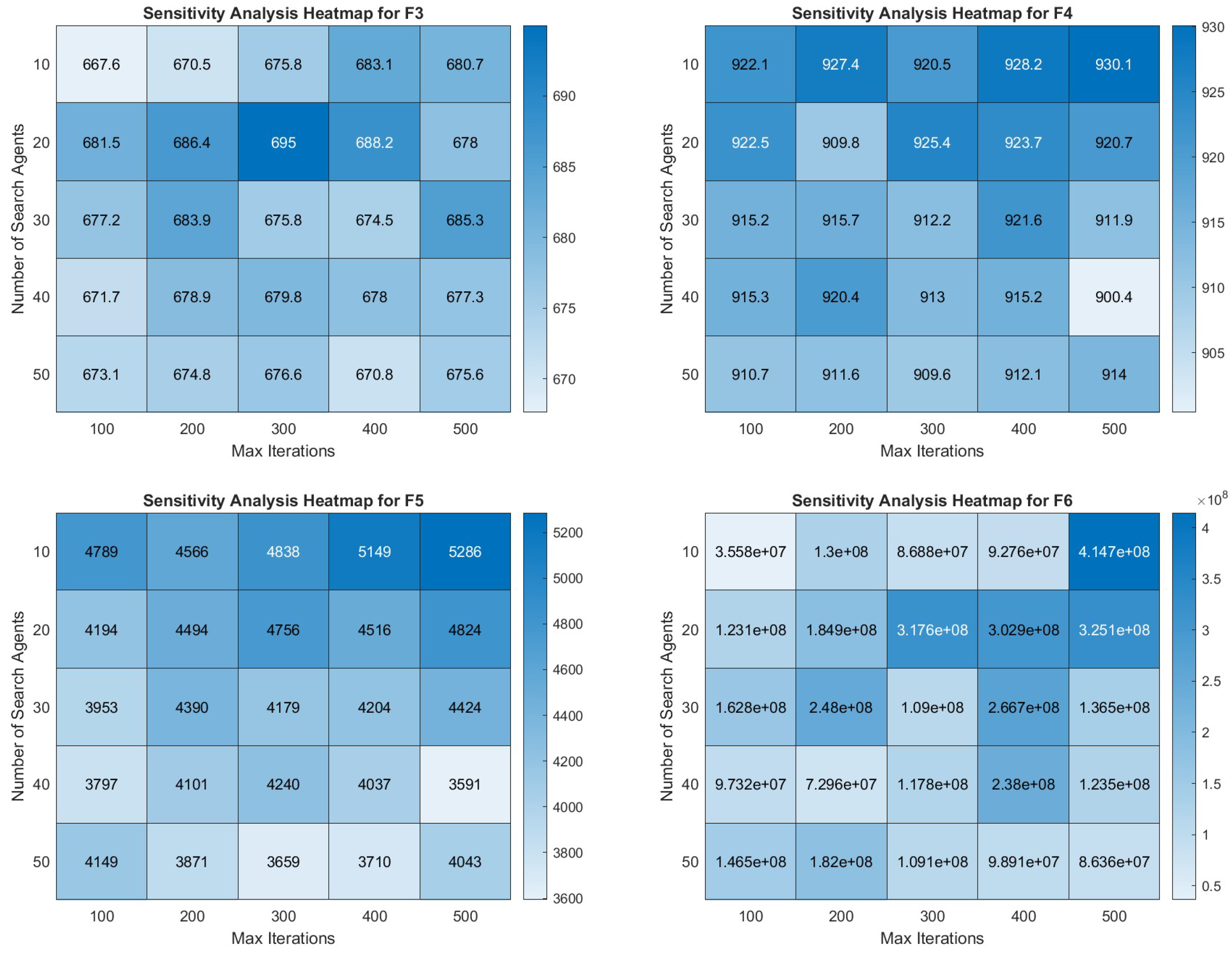
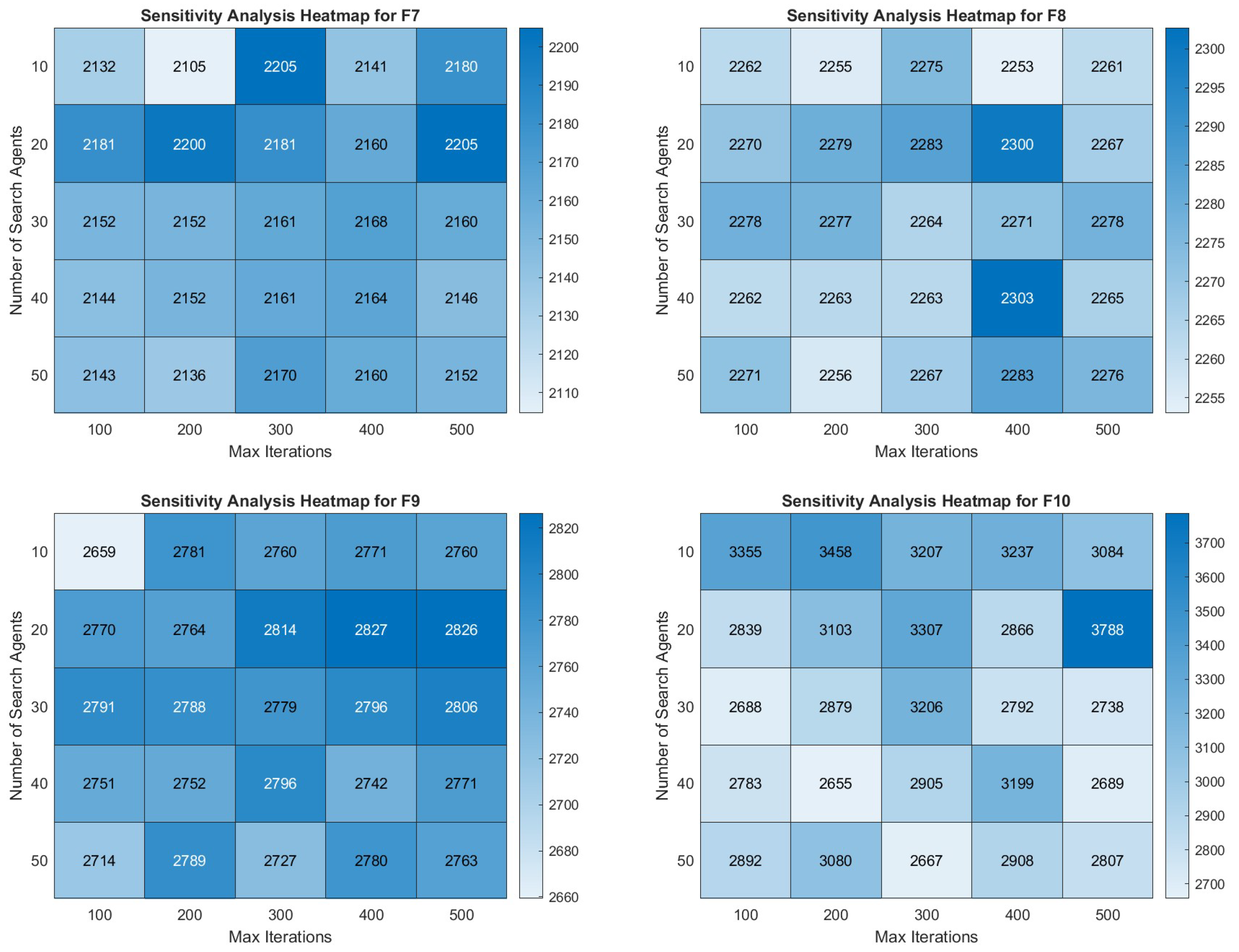

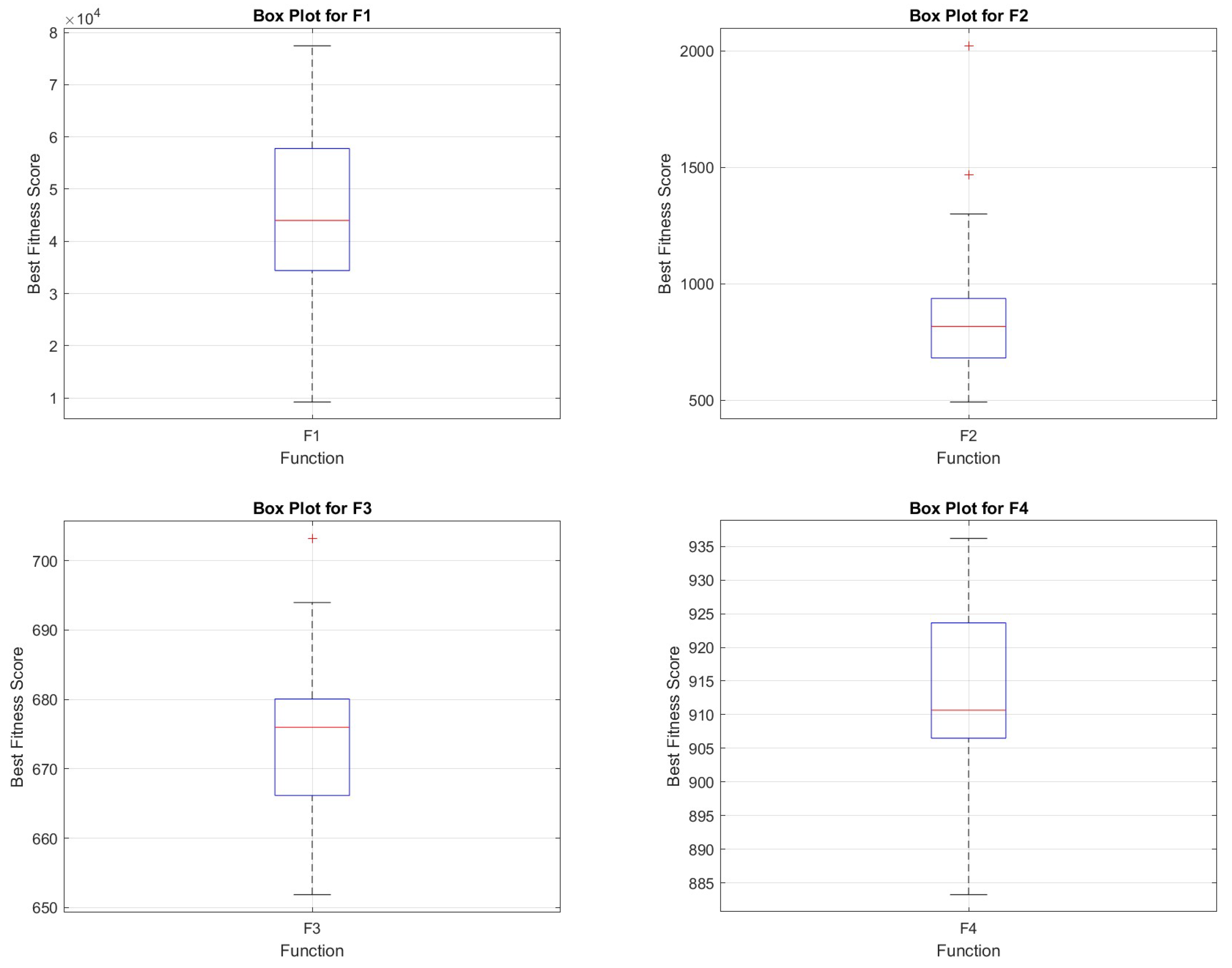
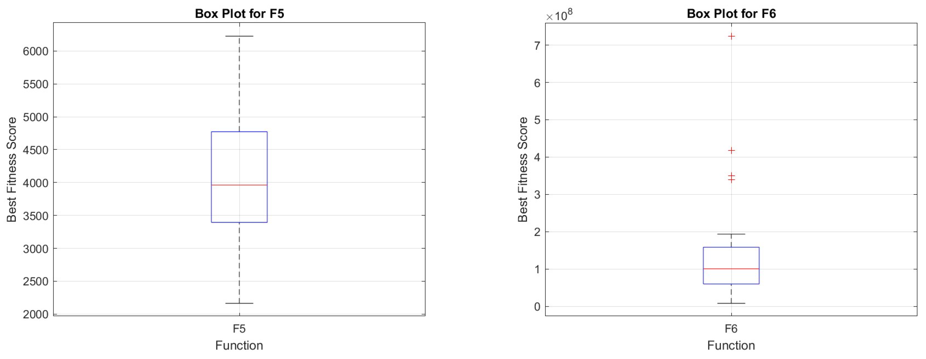
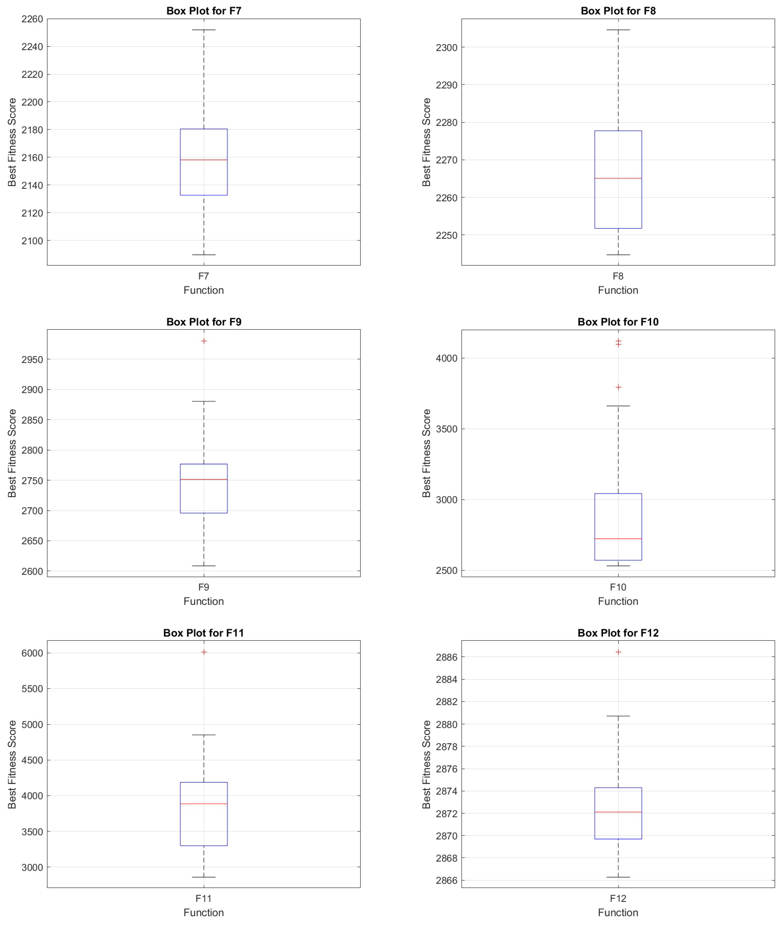
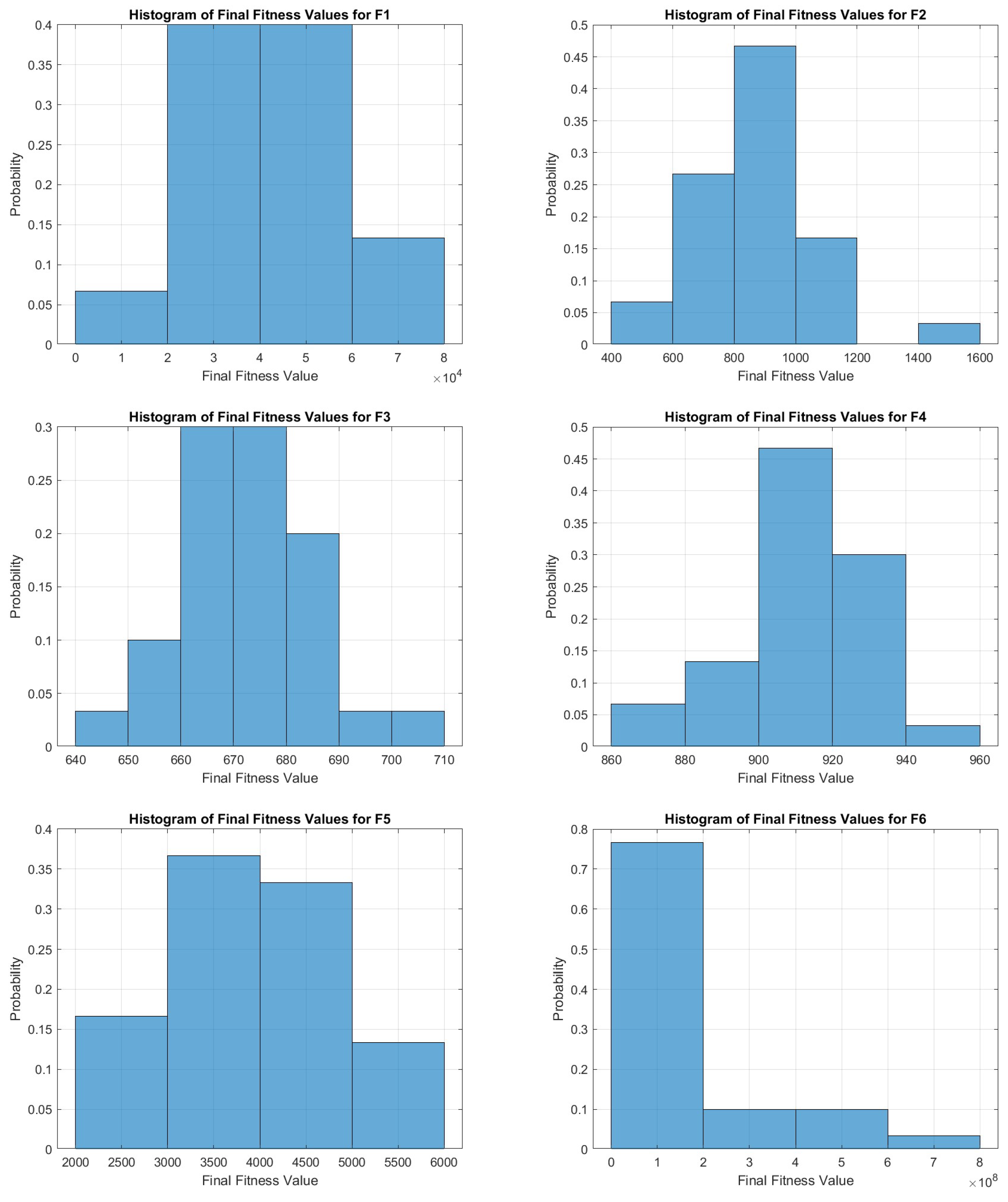

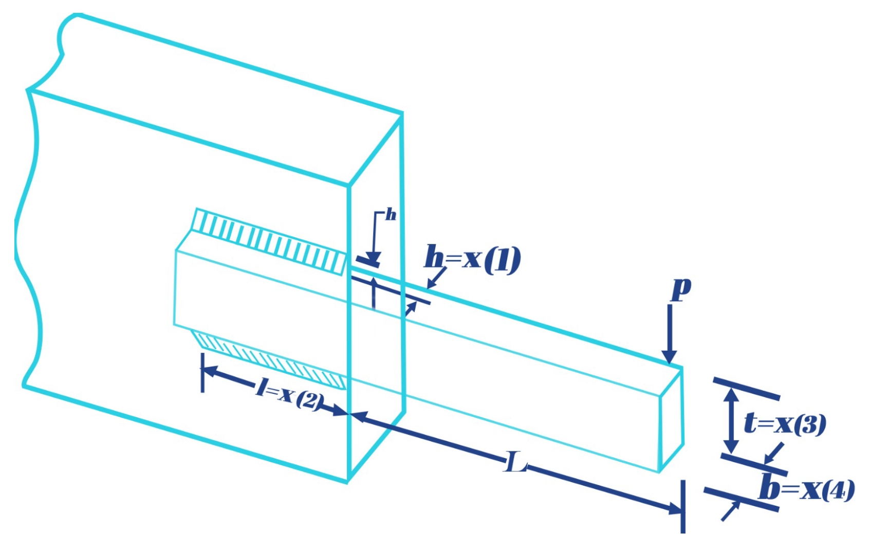

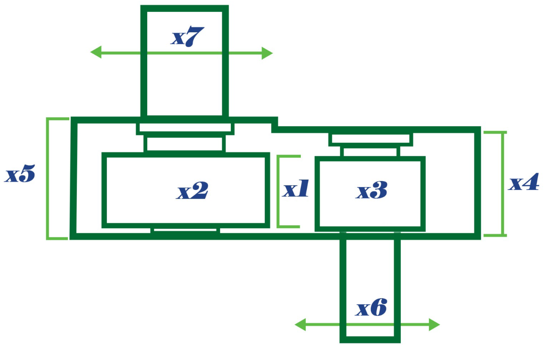
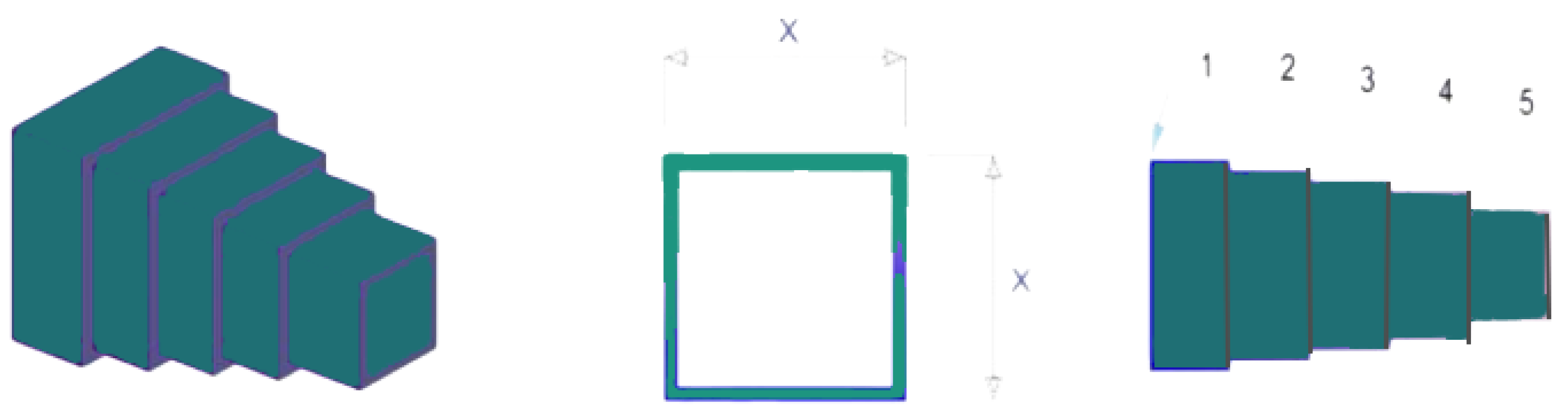
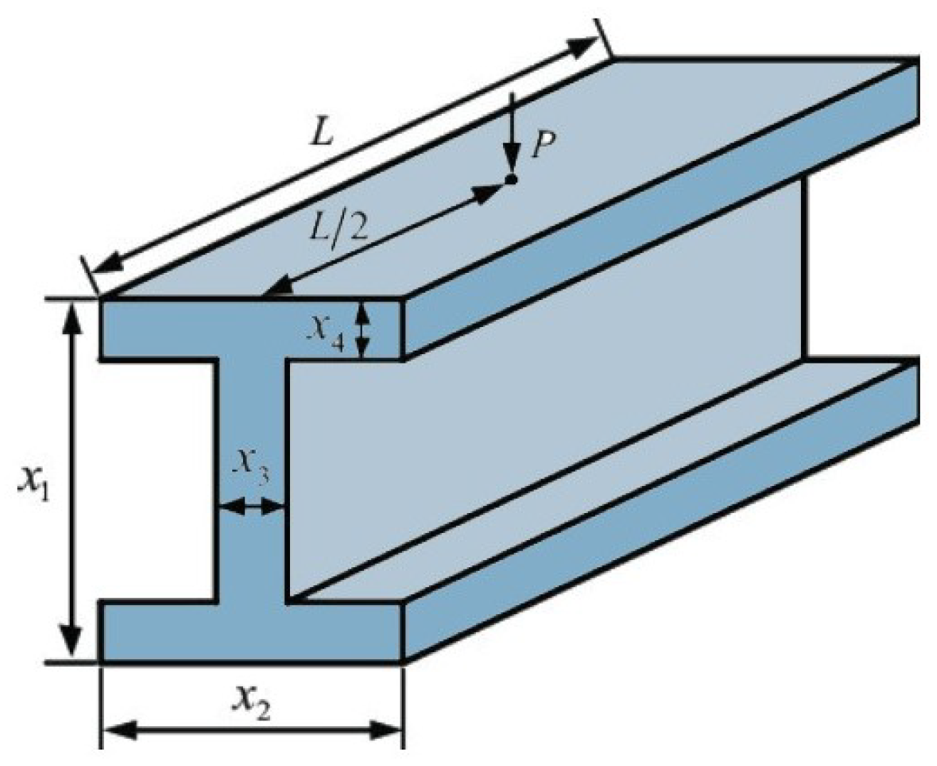
Disclaimer/Publisher’s Note: The statements, opinions and data contained in all publications are solely those of the individual author(s) and contributor(s) and not of MDPI and/or the editor(s). MDPI and/or the editor(s) disclaim responsibility for any injury to people or property resulting from any ideas, methods, instructions or products referred to in the content. |
© 2024 by the authors. Licensee MDPI, Basel, Switzerland. This article is an open access article distributed under the terms and conditions of the Creative Commons Attribution (CC BY) license (https://creativecommons.org/licenses/by/4.0/).