Post-Earthquake Emergency Logistics Location-Routing Optimization Considering Vehicle Three-Dimensional Loading Constraints

Abstract

An efficient humanitarian emergency logistics network is vital in responding to earthquake disasters. However, the asymmetric information inherent in the location and distribution stages can complicate the humanitarian emergency logistics network designing process, resulting in an asymmetric optimization problem. This paper addresses a multi-objective humanitarian emergency logistics network design problem during the earthquake response phase. The objective is to reduce societal expenses (e.g., logistical and deprivation costs) and mitigate risk to the logistics network by identifying ideal sites for distribution hubs, optimal emergency material distribution strategies, and precise material loading plans. The proposed model takes into account various constraint types, such as 3D loading limitations for relief materials, interruptions in distribution hubs, distribution centers’ capacity, transport vehicles’ capacity, and specific time windows for demand points. First, a multi-objective mixed-integer programming model is established to solve the problem. Uncertainty is modeled using a scenario-based probability approach. Second, a multi-objective genetic algorithm based on adaptive large neighborhood search (MOGA-ALNS) is designed to further optimize the solutions obtained from the evolutionary process using an adaptive large neighborhood search algorithm. Furthermore, the MOGA-ALNS integrates a simulated annealing process in the neighborhood search stage to inhibit the algorithm from reaching local optimums. Ultimately, the MOGA-ALNS is compared to three additional multi-objective optimization algorithms. The comprehensive analysis and discussion conducted unequivocally validate the competitiveness and efficacy of the proposed approach.

1. Introduction

The global occurrence of natural disasters has become increasingly common. Afghanistan experienced a 6.8 magnitude earthquake in June 2022, leading to around 1500 deaths and numerous injuries. A 7.8 magnitude earthquake close to the Turkey–Syria border in February 2023 resulted in more than 59,000 fatalities and economic damages surpassing 104 billion USD. Morocco endured a 6.8 magnitude earthquake in September 2023, resulting in close to 3000 fatalities and 6000 injuries. Afghanistan experienced back-to-back earthquakes of 6.2 magnitude in October 2023, leaving over 2000 people dead and close to 10,000 injured. Clearly, natural disasters, have resulted in considerable loss of life and extensive economic damage [1]. Adopting proactive measures has become a major concern for countries around the world looking to ensure that they are prepared to respond to sudden disasters [2].

The process of managing disasters generally encompasses four primary phases: mitigation, preparedness, response, and recovery [3]. The focus of this research is on the ‘response’ phase, which is typically characterized by three principal elements inherent in rescue missions: location, distribution, and routing. Challenges associated with the response phase and rescue missions arise from various elements, including cooperation between governmental and non-governmental entities, infrastructure breakdowns, destruction of transportation paths, and a critical lack of emergency resources [4,5,6,7]. Such elements might greatly affect decisions regarding emergency rescues, possibly resulting in the failure of humanitarian relief operations. Consequently, creating a dependable emergency logistics network (ELN) is crucial in ensuring the efficacy of rescue strategies, directly impacting the efficiency of rescue operations and the ultimate outcome of humanitarian relief.

Studies on ELNs have resulted in the formulation of diverse models that take into account aspects such as rescue expenses [8], equity [9], the duration of the rescue [10], and unpredictability [11]. However, the majority of these studies concentrated exclusively on factors such as location, routing, and allocation, paying minimal attention to emergency supply loading strategies. Items for emergency aid, including food, potable water, generators, fuel, tents, and blankets, differ greatly in their three-dimensional dimensions and frequently require concurrent transport to disaster zones, like generators with fuel, food with water, tents with blankets. However, the majority of current research has overlooked this facet of providing aid resources, resulting in a lack of understanding as to how to efficiently use scarce transportation space during emergencies [12,13]. Additionally, given that the present process of loading and unloading goods predominantly depends on manual labor and is not underpinned by scientific loading rules, loading schemes frequently depend on subjective elements, such as employees’ work experience and personal preferences [14,15]. However, because extant research has primarily focused on aspects such as cost and time efficiency, it has not adequately explored the optimization of loading schemes. Consequently, integrating loading schemes into the development of ELNs is vital in eliminating current research gaps and boosting the overall efficiency and effectiveness of rescue operations.

Compared to previous research, the location-routing optimization problem that loading schemes is more complex, necessitating the consideration of the distribution of demand points among multiple distribution centers, the allocation of vehicles to demand points, and the delivery routes vehicles might take. Furthermore, by employing the strategy of compartmentalization, the arrangement of items in a delivery system is decided by the order of demand points and the three-dimensional of goods. Additionally, when providing humanitarian aid following disasters, it is crucial to amalgamate principles of welfare economics to guarantee that logistics networks maximize benefits for most people [16]. Concurrently, it is crucial for the constructed logistics network to maintain utmost stability and dependability in settings susceptible to subsequent calamities. Moreover, we must consider disruptions to distribution centers, the capacity limitations and expansion of distribution centers, and delivery time windows required by demand points to more accurately reflect post-disaster scenarios in the real world.

Given the aforementioned conditions, this paper studies the humanitarian emergency logistics location-routing problem, optimizing location, routing, and loading plans while adhering to three-dimensional loading and resource constraints, and aims to minimize both social costs and the risk to the logistics network. The primary contributions of this paper are as follows:

(1)

A multi-objective location-routing problem with a three-dimensional loading constraints optimization model is formulated. This model is unique in that it optimizes distribution centers, vehicle scheduling, and loading plans while considering three-dimensional loading constraints, facility disruptions, capacity limitations and expansions, and time window constraints while balancing social costs (logistical and deprivation costs) and risk to the logistics network. By integrating these two goals, the model not only enhances resource allocation efficiency but also strengthens the reliability of the ELN.

(2)

A multi-objective mixed genetic algorithm (MOGA) based on adaptive large neighborhood search (ALNS) is proposed. This MOGA-ALNS employs ALNS for neighborhood search, with five removal and insertion operators designed to enhance the diversity and flexibility of the search process, effectively preventing convergence to local optima. Simultaneously, it leverages the global search capability of genetic algorithms to ensure the diversity and comprehensiveness of the solutions.

The paper is organized as follows: Section 2 provides an overview of the extant literature on the topic. Section 3 delves into the research issue and outlines the mathematical model. Section 4 presents the proposed solution to the issue. The numerical experiments performed are reported in Section 5. Section 6 concludes this study and suggests future research directions.

2. Literature Review

2.1. Emergency Logistics Network

In contrast to conventional logistics systems, an ELN must account for potential interruptions in its operations. The design of an ELN mainly encompasses two elements: infrastructure (e.g., distribution centers, hospitals, and shelters) and pathways. An ELN primarily focuses on optimizing the facility location and distribution route. Scholarly works on the optimization of facility locations have primarily concentrated on identifying the ideal quantity and placement of facilities for construction, while choices regarding distribution paths have mainly been associated with the design of transportation routes.

Crafting an ELN that ensures both high efficiency in delivery and reduced costs necessitates the strategic selection of suitable locations [17,18]. Yang et al. [19] tackled the unpredictability of emergency needs and the timing of resource distribution in disasters by creating a multi-stage facility location model aimed at improving overall cost efficiency and equity and by devising an algorithm based on Benders for branch and bound. Men et al. [20] formulated a multi-objective location model for pinpointing facilities in the management of disastrous chain chemical incidents. The model takes into account not just the spatial attributes of facilities but also addresses pertinent potential hazards. A multi-objective evolutionary algorithm was developed to address this issue. Wang et al. [21] developed a distributionally robust optimization model for optimizing the locations of distribution centers and backup warehouses, as well as the distribution of relief supplies in an ELN, by minimizing expected total costs and total delivery times. Their proposed solution was a Benders decomposition-based exact algorithm.

Some studies on facility locations have considered the possibility of facility disruptions. Maliki et al. [21] formulated a multi-phase model for locating facilities during crises characterized by extremely unpredictable demands. Their goal was to reduce overall expenses and CO₂ emissions, suggesting a comprehensive optimization strategy utilizing the non-dominant sorting genetic algorithm. Wang et al. [22] tackled the complex issue of locating facilities amid uncertainty, developing two key functions: ensuring coverage reliability and calculating the overall cost. In response to this issue, a bi-population-oriented evolutionary algorithm was suggested. Zhang et al. [23] explored the reliable issue of location inventory, taking into account the reciprocal interplay between failures in the simultaneous placement of forward and reverse distribution centers within a closed-loop supply chain. The likelihood of interruptions varied based on the types of facilities, with the goal being to reduce overall expenses. Their suggestion was a decomposition approach based on the dominance-based outer approximation algorithm.

Numerous studies have tackled issues related to the distribution of supply routes in urgent situations [24,25,26]. Molina et al. [27] presented an adaptable multi-objective algorithm for searching large neighborhoods, aimed at reducing vehicle count, overall travel expenses, and the greatest delay in addressing the rescue vehicle routing issue. Khanchehzarrin et al. [28] developed a dual-layered disaster location-routing model with multiple goals, taking into account the risk to supplies. For improved problem-solving, the bi-level multi-objective model was converted into a single-level, single-objective model through the application of the epsilon-constraint method and Karush–Kuhn–Tucker conditions. Wang et al. [29] introduced a two-level emergency vehicle routing problem with time windows in a closed area, aiming to minimize total operating costs, total delivery time, and the number of vehicles. They designed a multi-objective ALNS segmentation algorithm as a proposed solution.

2.2. Integrating Research on Delivery Route Optimization and Three-Dimensional Packing Constraints (VRPTDLCs)

Due to the limited research on the integration of the location-routing problem (LRP) and three-dimensional packing constraints, this section analyzes the current status of research on LRP-related issues, primarily the vehicle routing problem with three-dimensional loading constraints (VRPTDLCs). Whether in emergency relief scenarios or in the daily logistics industry, the types of materials for distribution are extremely diverse. This also means that their sizes are inevitably different. Because as many goods as possible with given sizes and weights must be loaded into a vehicle before delivery to serve more demand points, it is necessary to determine through an optimization process whether these goods can be successfully loaded. Reil et al. [30] studied a vehicle routing problem, considering vehicle return trips, time windows, and 3D packing constraints. They created a bi-objective model aimed at reducing the quantity of transport vehicles and shortening the travel distance. The researchers formulated a hybrid method that merges taboo search with an evolutionary algorithm, targeting the improvement of vehicle routing and freight loading strategies. Furthermore, Göçmen et al. [31] presented the challenge of selecting routes for a multimodal transport network, taking into account three-dimensional loading limitations. To address this issue, they developed a mixed-integer programming model, aiming to reduce both transportation expenses and the vehicle count. Specifically, they employed a mixed algorithm, integrating k-means, machine learning, and genetic algorithms.

In the examination of three-dimensional packing constraints, various practical loading considerations are commonly taken into account. These include the necessity for load stability, the requirement for a minimum support area, and the adherence to last-in-first-out (LIFO) loading principles [32]. In addition, some variants of VRPTDLC have also attracted scholarly attention. Männel et al. [33] studied a pickup and delivery route problem that considers three-dimensional packing constraints with the objective of minimizing transportation distance. A combination of tree search and large neighborhood search was employed in their hybrid algorithm to effectively address and optimize the issue. In a separate study, Rajaei et al. [34] tackled a multifaceted real-world challenge that merges the vehicle routing issue with the use of heterogeneous vehicles and three-dimensional packing limitations. They developed a heuristic algorithm based on column generation to determine the most cost-effective set of transportation routes.

2.3. Compartmentalization Strategies for Vehicles

In the realm of practical transport, dividing vehicle compartments into multiple sections for carrying diverse goods is seen as an efficient approach to handling the distribution of goods of varying types and sizes [35]. This approach essentially involves segmenting a vehicle’s load area into a finite number of sections, each designated for a specific kind of cargo. Historically, vehicle compartmentalization has been applied in scenarios such as the transportation of various temperature-sensitive food items (e.g., frozen, fresh, and ambient products) to supermarkets [36], the delivery of assorted petroleum products (e.g., diesel and gasoline) to fuel stations [37], or the segregation of different kinds of waste (e.g., colored glass waste) [38,39]. Yahyaoui et al. [37] explored a scenario where a specialized fleet with numerous compartmental spaces was designed to transport varied types of fuel from a central warehouse to several gas stations. Zbib and Laporte [38] investigated the application of compartmentalization in roadside waste collection, creating a mathematical model to reduce travel costs, and, ultimately, putting forth a tri-stage algorithm. Yang et al. [39] devised a compartmentalization approach for city-wide solid waste collection, proposing that each vehicle’s capacity be divided into limited sections, each tailored for a specific waste type. Their findings indicated that cost efficiencies increase with an increase in the number of compartments. To sum up, vehicle compartmentalization offers substantial benefits in distributing diverse goods, yet its application in humanitarian emergency logistics has lacked extensive academic exploration.

In order to further elucidate the differences between this study and existing research, and to define the contributions of this research,

Table 1. Summary of the literature pertaining to ELN.

Reference	Location	Allocation	Objective	Vulnerable Section		Key Constraints				Solution
				Facility	Link	Fac. Cap	Fac. Exp	TWs	3D Loading
Mohammadi et al. (2020) [40]	$\surd$	$\surd$	Total cost Makespan Transport cost bounds variation	$\surd$		$\surd$				Exa
Wei et al. (2020) [41]	$\surd$	$\surd$	Total cost Demand satisfaction			$\surd$		$\surd$		Met
Li et al. (2020) [42]	$\surd$	$\surd$	Total cost			$\surd$				Exa
Sun et al. (2021) [43]	$\surd$	$\surd$	Total cost Injury severity score							Exa
Gao et al. (2021) [44]		$\surd$	Fairness Makespan		$\surd$	$\surd$				Exa
Abazari et al. (2021) [45]	$\surd$	$\surd$	Total cost Makespan							Met
Cheng et al. (2021) [46]		$\surd$	Fairness			$\surd$				Exa
Alem et al. (2021) [47]	$\surd$	$\surd$	Effectiveness			$\surd$	$\surd$			Exa
Peng et al. (2022) [48]	$\surd$	$\surd$	Total cost Demand satisfaction					$\surd$		Met
Ghasemi et al. (2022) [49]	$\surd$	$\surd$	Total costs Maximum number of unsatisfied demands		$\surd$	$\surd$				Met
Vosooghi et al. (2022) [50]	$\surd$	$\surd$	Total cost Response time			$\surd$	$\surd$			Met
Bayraktar et al. (2022) [51]	$\surd$	$\surd$	Total cost							Met
Wang et al. (2023) [52]	$\surd$	$\surd$	Total cost Makespan	$\surd$		$\surd$				Exa
Meng et al. (2023) [10]	$\surd$	$\surd$	Total cost Makespan	$\surd$	$\surd$					Exa
Yang et al. (2023) [19]	$\surd$	$\surd$	Total cost Fairness			$\surd$				Exa
Wang et al. (2023) [9]	$\surd$	$\surd$	Time cost Quantity of short supplies		$\surd$	$\surd$				Heu
Sheikholeslami et al. (2023) [53]	$\surd$	$\surd$	Total cost Coverage of the network			$\surd$				Met
Li et al. (2023) [54]	$\surd$	$\surd$	Total cost in the worst case	$\surd$						Heu
Zhang et al. (2023) [11]	$\surd$	$\surd$	Total cost			$\surd$				Meta
Yang et al. (2024) [55]	$\surd$	$\surd$	Total cost	$\surd$		$\surd$				Exa
This study	$\surd$	$\surd$	Total cost Risk of network	$\surd$	$\surd$	$\surd$	$\surd$	$\surd$	$\surd$	Met

Note: Fac. Cap = Facility capaicity, Fac. Exp = Facility expansion, TWs = Time windows, Exa = Exact, Met = Metaheuristic, Heu = Heuristic.

lists the relevant research works and their main characteristics. By summarizing the relevant studies, this review yielded the following insights: (1) Currently, most research on humanitarian emergency logistics has focused on cost and time; however, in practice, the reliability of distribution networks constructed for emergency resource distribution is crucial; (2) There is a gap in the literature on facility location, distribution route, and loading scheme optimization, resulting in insufficient attention to the intersecting issues connecting these three aspects; (3) Metaheuristic algorithms have been widely and successfully used to address related issues in the VRPTDLC; (4) Given the inefficiency of traditional metaheuristic algorithms in solving complex problems, scholars have generally designed hybrid algorithms as potential solutions.

Given the above, this paper proposes a multi-objective location-routing problem model for humanitarian emergency logistics in the event of facility disruptions in natural disaster scenarios. This model takes into account the unique challenges associated with disaster environments, such as the location of distribution centers, vehicle routing, and the three-dimensional packing of relief supplies. Additionally, a hybrid algorithm composed of an improved ALNS algorithm and a genetic algorithm is designed to solve this problem.

3. Model Formulation

3.1. Problem Description

The ELN in this study comprises a set of demand points, multiple candidate distribution centers with capacity limits, and interconnected roadways. Each demand point has a specific delivery time window, deviations from which incur penalties. The supply needs at these demand points are diverse, with each item having well-defined attributes. Despite capacity limitations, the distribution centers the distribution centers can undergo a certain degree of capacity expansion. Post-earthquake, the operation of some distribution centers may be disrupted, meaning these distribution centers cannot be considered in location-allocation. Additionally, the risk from secondary natural disasters, such as aftershocks, continues to affect both the operational distribution centers and roadways.

In the optimization of cargo loading, a carriage segmentation strategy is adopted for efficiency. The space in a vehicle is divided into compartments for different material types. While meeting three-dimensional loading constraints, goods of the same category are placed in the same carriage according to the LIFO principle while adhering to the delivery sequence of the demand points.

In practice, the construction of ELNs needs to consider multiple factors. Social and deprivation costs can indirectly reflect the efficiency of the entire emergency logistics system. Therefore, this model aims to minimize total rescue transportation costs (including location, expansion, transportation, vehicle usage, and time penalty-related costs). Additionally, given the risks of facility interruption and road damage, choosing a lower-risk ELN is vital. A network that does not consider risk values might lead to severe losses in cases of secondary disasters. Thus, this study aims to minimize both risk and total cost in location-routing schemes.

To illustrate, Figure 1 shows an example with four distribution centers (A, B, C, and D) and nine demand points. Post-earthquake, Center B is disrupted, leaving A, C, and D. Centers A and C are chosen for supply distribution. However, the original capacity of Center C is insufficient in fulfilling the demand volume of the demand points, necessitating a certain degree of capacity expansion. The final result is presented as the location-routing scheme depicted in Figure 1. Figure 2 presents a feasible loading plan for the transport route 2-1-9 in Figure 1.

3.2. Symbols

$G=(V,A)$ is an undirected network, where $V$ is the set of nodes consisting of a subset $I$ of candidate distribution center locations and a subset $J$ of geographically dispersed demand points; $A=\left\{\left.\left(\mathrm{i},j\right)\right|\mathrm{i},\mathrm{i}\in V,i\ne j\right\}$ is the set of arcs connecting every pair of nodes in $V$; $K=\left\{k|k=\mathrm{1,2},\cdots h\right\}$ is the set of available distribution vehicles; and $S=\left\{\left.s\right|s=\mathrm{1,2},\cdots ,p\right\}$ is a set of scenarios, each scenario specifying a set of simultaneously disrupted distribution centers.

Table A1. Indices, parameters, and decision variables utilized in the formulated model.

Notation	Description
Indices
$I$	Set of candidate distribution centers; $I=\left\{\left.i\right|i=1,\cdots ,n\right\}, n$ indicates the number of candidate distribution centers.
$J$	Set of demand points; $J=\left\{\left.j\right|j=n+1,\cdots ,n+m\right\}, m$ represents the number of demand points.
$V$	Set of distribution centers and demand points; $V=I\cup J$.
$A$	Set of segments in the distribution network; $A=\left\{\left.\left(i,j\right)\right|i, j\in V, i\ne j\right\}, i$, and $j$ represent nodes in the network.
$K$	Set of distribution vehicles; $K=\left\{k|k=\mathrm{1,2},\cdots h\right\}, h$ represents the total count of vehicles.
$S$	Set of scenarios; $S=\left\{\left.s\right|s=\mathrm{1,2},\cdots ,p\right\},$ where $p$ represents the number of scenarios, each of which has a set of distribution centers experiencing a simultaneous disruption.
$N_k$	Set of demand points for vehicle $k$ services; $k\in K$.
$C$	Set of goods types needed across all demand points; $C=\left\{\left.c\right|c=1,\dots ,l\right\},$ where $l$ denotes the $lth$ type of goods.
$D_k$	Set of spaces in the distribution vehicle compartment of vehicle $k, D_k=\left\{\left.d\right|d=1,\dots ,q\right\}$, $k\in K,$ and $q$ is the overall count of spaces.
$G$	Set of goods placed in the same space of the same vehicle with good $c_{kdju}^s$ and overlapping with the under-plane projection of goods in scenario $s,G\left\{c_{kdjv}^s\right|\forall c\in C, s\in S, k\in K, d\in D_k, i,j\in J,1\le v\le m_{kd}^s and if i=j,v\ne u\}$.
$U$	Set of goods placed in the same space of the same vehicle with good $c_{kdju}^s$ and the bottom surface of good $c_{kdju}^s$ is at the same height in scenario $s,$$U=\left\{c_{kdjv}^s\right|c_{kdjv}^s\in G, {\overline{z}}_{C_{skdiu}}={\underset{\_}{z}}_{{ C}_{skdiu}}\}$.
Parameters
${\delta }_{ij}$	Distance between the depot or demand point i and demand point j, $i, j\in I\cup J$.
${\beta }_i$	The base capacity of the distribution center $i, i\in I$.
${\mu }_i$	The maximum capacity of the distribution center $i$ can be expanded, $i\in I$.
${\gamma }_i$	The cost of constructing the distribution center $i, i\in I$.
$e_i$	The unit expansion cost of the distribution center $i, i\in I$.
$f$	Fixed operating cost of the vehicle.
$\tau$	The cost per unit distance traveled by the vehicle.
$\nu$	The speed of vehicles.
$O$	The maximum loading volume of the vehicle.
$B$	The maximum load capacity of the vehicle.
${layer}_{kd}^s$	The actual count of layers of goods loaded in the $dth$ space of vehicle $k, k\in K, d\in D_k$.
${row}_{kd}^s$	The actual count of rows of goods loaded in the $dth$ space of vehicle $k, k\in K, d\in D_k$.
${column}_{kd}^s$	The actual count of columns of goods loaded in the $dth$ space of vehicle $k, k\in K, d\in D_k$.
$m_{kd}^s$	The count of goods placed within the $dth$ space of vehicle $k$ in scenario $s, s\in S, k\in K, d\in D_k$.
$m_{kdj}^s$	The number of goods loaded at demand point $j$ within region $d$ by delivery vehicle $k$ in scenario $s, s\in S, k\in K, d ϵ{ D}_k, j\in J$.
$q_{kd}^s$	The individual quality of the goods loaded in region $d$ by delivery vehicle $k, k\in K, d\in D_k$.
$Q_{kd}^s$	The overall quality of goods placed in the $dth$ space of vehicle $k, k\in K, d\in D_k$.
${\sigma }_{kd}^s$	The overall size of goods placed in the $dth$ space of vehicle $k, k\in K, d\in D_k$.
$c_{kdiu}^s$	The overall number of goods placed in the $dth$ space of vehicle $k, k\in K, d\in D_k$.
$L,W,H$	The dimensions of the carriage, including its length, width, and height..
$l_{kd},w_{kd},h_{kd}$	The length, width, and height of the $dth$ space of vehicle $k, k\in K, d\in D_k$.
$l_{kd}^s,{ w}_{kd}^s,{ h}_{kd}^s$	The length, width, and height of the goods loaded in the $dth$ space of vehicle $k, c\in C, k\in K, d\in D_k$.
$\left({\overline{x}}_{{ C}_{skdju}},{\overline{y}}_{{ C}_{skdju}},{\overline{z}}_{{ C}_{skdju}}\right)$	The coordinate at the upper-right corner of the front side of the $uth$ carriage of the $ith$ point in the $dth$ space of vehicle $k, c\in C, k\in K, d\in D_k, j\in J, 1\le u\le m_{kd}^s$.
$\left({\underset{\_}{x}}_{{ C}_{skdju}},{\underset{\_}{y}}_{{ C}_{skdju}},{\underset{\_}{z}}_{{ C}_{skdju}}\right)$	The coordinate at the lower-left corner of the back side of the $uth$ carriage of the $ith$ point in the $dth$ space of vehicle $k, c\in C, k\in K, d\in D_k, j\in J, 1\le u\le m_{kd}^s$.
$P_s$	The probability of scenario $s$ occurring, $s\in S$.
$P_{1i}^s$	The probability of secondary disasters such as aftershocks occurring at the distribution center $i, i\in I, s\in S$.
$P_{2i}^s$	The probability of huge losses caused by disasters such as aftershocks affecting the distribution center in scenario $s, s\in S, i\in I$.
${\lambda }_{1i}^s$	The cost of losses incurred by distribution center $i$ due to disaster risks such as aftershocks in scenario $s, s\in S, i\in I$.
$P_{1ij}^s$	The probability of transportation risk associated with the route section $\left(i, j\right)$ in scenario $s, i, j\in A$.
$P_{2ij}^s$	The probability of significant loss of goods due to transportation risk occurring along route segment $(i, j)$ in scenario $s, i, j\in A$.
${\lambda }_{2i}^S$	The cost of loss due to transportation risk when goods are transported from $i$ to $j$ in scenario $s, i, j\in A$.
${\eta }_{ijk}^s$	The cargo load of vehicle $k$ when transporting from $i$ to $j$ in scenario $s, i, j\in I\cup J, k\in K, i\ne j.$
$t_{jk}^s$	The time for vehicle $k$ to reach point $j$ in scenario $s, s\in S, j\in J, k\in K$.
${\psi }_{jk}^s$	The time vehicle $k$ requires to serve demand point $j$ in scenario $s, s\in S, j\in J, k\in K$.
${\phi }_j^e$	The penalty coefficient for vehicles arriving at demand point $j$ ahead of schedule, $j\in J$.
${\phi }_j^l$	The penalty coefficient for vehicles arriving at demand point $j$ behind schedule, $j\in J$.
$T_{1j}^s$	The earliest acceptable service time for demand point $j, j\in J$.
$T_{2j}^s$	The latest acceptable service time for demand point $j, j\in J$.
${\xi }_i^s$	The value is 1 if distribution center $i$ fails in scenario $s$; otherwise, it is 0, $s\in S, i\in I$.
${\omega }_{kdc}$	The value is 1 if vehicle $k$ is loaded with class $c$ goods within region $d$; otherwise, it is 0, $k\in K, c\in C, d\in D_k$.
Decision variable
$x_i^s$	The value is 1 if a distribution center is established at location $i$ in scenario $s$; otherwise, it is 0, $s\in S, i\in I$.
$y_{ijk}^s$	The value is 1 if vehicle $k$ travels from node $i$ to node $j$ in scenario $s$; otherwise, it is 0, $s\in S, i, j\in I\cup J, k\in K, i\ne j$.
$z_{ij}^s$	The value is 1 if demand point $j$ is serviced by distribution center $i$ in scenario $s$; otherwise, it is 0, $s\in S, i\in I, j\in J.$
${\gamma }_{kdj}^s$	The value is 1 if vehicle $k$ carries the goods of demand point $j$ within region $d$; otherwise, it is 0, $s\in S, j\in J, k\in K, d\in D$k..
${\Omega }_{ik}^s$	The value is 1 if vehicle $k$ departs from distribution center $i$ to provide delivery services in scenario $s$; otherwise, it is 0, $s\in S, i\in I, k\in K$.
${\zeta }_i^s$	The capacity expansion amount of distribution center $i$ in scenario $s, s\in S, i \in I$.

provides the parameters and decision variables required for the formulated mathematical model.

3.3. Emergency Logistics Network Risk Measurement Formula

Wang and Sun [56] defined the formula for measuring the risk of ELNs as:

$$Risk=Probabiliity\left(P\right)\times Vulenrability\left(V\right)\times Loss\left(L\right)$$

(1)

where $P$ symbolizes the likelihood of risk during humanitarian aid, taking into account factors such as road destruction, route intricacy, climatic conditions, and the chance of a subsequent disaster. $V$ symbolizes the likelihood of substantial losses following the aforementioned risks, influenced by factors such as geographic position, population and building density, traffic volume, and the significance and worth of the transported materials. $L$ denotes both the immediate and secondary impacts of the risk, encompassing financial damages and fatalities. Within Wang and Sun’s [56] particular research framework, the comprehensive risk examined is bifurcated into two segments: the hazard encountered during transit and the hazard associated with road upkeep. However, in actual relief operations, aside from the various risks on the road, there is also the risk of secondary disasters occurring at distribution centers. In view of this, this study modified the above formula to better fit real-world scenarios:

$$Risk=\sum _{s\in S}{P}_s\left[\sum _{\mathrm{i}\in I}{P}_{1i}^s·P_{2i}^s·{\lambda }_{1i}^S·x_i^s+\sum _{\mathrm{i}\in A}\sum _{j\in A}\sum _{k\in K}{P}_{1ij}^s·{pP}_{2ij}^s·{\lambda }_{2ij}^S·y_{ijk}^s\right]$$

(2)

where $P_{1i}^s·P_{2i}^s·{\lambda }_{1i}^S$ represents the risk of secondary disasters occurring at distribution centers, and $P_{1ij}^s·P_{2ij}^s·{\lambda }_{2ij}^S$ represents risks that might occur during the distribution transportation process in the humanitarian relief chain.

3.4. Mathematical Model

The objective function serves as the foundation for determining how conflicting objectives are coordinated and how scarce resources are optimally allocated. If a model does not establish a relationship that reflects the real system, its ability to generate reasonable recommendations is compromised. Moreover, reducing logistics costs to a minimum without considering the magnitude of distribution plan risks can have adverse effects on the people in the disaster-affected area. Therefore, this model simultaneously considers the minimization of the total cost (site location cost of distribution centers, expansion costs, transportation costs, vehicle usage costs, and time penalty costs) and the risk value of the logistics network. Subsequently, the following optimization model is formulated:

$$Min{ Z}_1=\sum _{s\in S}{P}_s\left[\begin{array}{c}{\displaystyle \sum _{i\in I}}{x}_i^s·{\gamma }_i+{\displaystyle \sum _{i\in I}}{\delta }_i^s·e_i+{\displaystyle \sum _{i\in I}}{\displaystyle \sum _{j\in J}}{\displaystyle \sum _{k\in K}}{y}_{ijk}^s·f+{\displaystyle \sum _{i\in A}}{\displaystyle \sum _{j\in A}}{\displaystyle \sum _{k\in K}}{y}_{ijk}^s·{\delta }_{ij}·\tau \\ +{\displaystyle \sum _{j\in J}}{\displaystyle \sum _{k\in K}}\left\{{\phi }_j^e·max\left(T_{1j}^s-t_{jk}^s,0\right)+{\phi }_j^e·max\left(t_{jk}^s-T_{2j}^s,0\right)\right\}\end{array}\right]$$

(3)

$$Min{ Z}_2=\sum _{s\in S}{P}_s\left[\sum _{i\in I}{P}_{1i}^s·P_{2i}^s·{\lambda }_{1i}^S·x_i^s+\sum _{i\in A}\sum _{j\in A}\sum _{k\in K}{P}_{1ij}^s·P_{2ij}^s·{\lambda }_{2ij}^S·y_{ijk}^s\right]$$

(4)

$$\sum _{i\in I}{z}_{ij}^s=1,\forall j\in J,\forall s\in S$$

(5)

$$\sum _{i\in V}\sum _{k\in k}{y}_{ijk}^s=1,\forall j\in J,\forall s\in S$$

(6)

$$y_{ijk}^s\le x_i^s,\forall i\in I,\forall j\in J,\forall k\in K,\forall s\in S$$

(7)

$$\sum _{j\in J}\sum _{k\in k}{y}_{ijk}^s\ge x_i^s,\forall i\in I,\forall s\in S$$

(8)

$$\sum _{i\in I}\sum _{j\in J}{y}_{ijk}^s\le 1,\forall k\in K,\forall s\in S$$

(9)

$$\sum _{j\in V}{y}_{ijk}^s=\sum _{j\in V}{y}_{ijk}^s,\forall i\in V,\forall k\in K,\forall s\in S$$

(10)

$$\sum _{j\in J}{y}_{ijk}^s={\Omega }_{ik}^s,\forall i\in I,\forall k\in K,\forall s\in S$$

(11)

$$\sum _{i\in I}\sum _{j\in J}{y}_{ijk}^s\le \left|S\right|-1,\forall i\in I,\forall k\in K,\forall s\subseteq V$$

(12)

$${\beta }_i·x_i^s+{\delta }_i^s\le {\mu }_i,\forall i\in I,\forall s\in S$$

(13)

$$\sum _{k\in K}\sum _{d\in D_k}{Q}_{kd}^s·m_{kd}^s{·\Omega }_{ik}^s\le {\beta }_i·x_i^s+{\delta }_i^s,\forall i\in I,\forall s\in S$$

(14)

$$\sum _{d\in D_k}{q_{kd}^s·m}_{kd}^s=Q_{kd}^s,\forall k\in K,\forall s\in S$$

(15)

$$\sum _{d\in D_k}{Q}_{kd}^s\le O,\forall k\in K,\forall s\in S$$

(16)

$$\sum _{d\in D_k}{l_{kdc}^s·w_{kdc}^s·h}_{kdc}^s·m_{kd}^s={\sigma }_{kd}^s,\forall k\in K,\forall s\in S$$

(17)

$$\sum _{d\in D_k}{\sigma }_{kd}^s\le B,\forall k\in K,\forall s\in S$$

(18)

$$t_{jk}^s{=\left(t_{ik}^s+{\psi }_{jk}^s+{\delta }_{ij}/\nu \right)·y}_{ijk}^s,\forall i\in I,\forall s\in S$$

(19)

$$\sum _{i\in V}{\eta }_{ijk}^s=\sum _{i\in V}{\eta }_{jik}^s+\sum _{d\in D_k}{q_{kd}^s·m}_{kdj}^s,\forall j\in J,\forall k\in K,\forall s\in S$$

(20)

$$\sum _{j\in J}{m}_{kdj}^s·{\epsilon }_{kdj}^s=m_{kd}^s,\forall k\in K,d\in D_k,\forall s\in S$$

(21)

$${\underset{\_}{x}}_{{ C}_{kdjus}}\ge 0,\forall k\in K,\forall d\in D_k,\forall j\in J,\forall s\in S,\forall c\in C,1\le u\le m_d^k$$

(22)

$${\underset{\_}{y}}_{{ C}_{kdjus}}\ge 0,\forall k\in K,\forall d\in D_k,\forall j\in J,\forall s\in S,\forall c\in C,1\le u\le m_d^k$$

(23)

$${\underset{\_}{z}}_{{ C}_{kdjus}}\ge 0,\forall k\in K,\forall d\in D_k,\forall j\in J,\forall s\in S,\forall c\in C,1\le u\le m_d^k$$

(24)

$${layer}_{kd}^s{·h}_{dc}^k\le h_d,\forall k\in K,\forall d\in D_k,\forall s\in S,\forall c\in C$$

(25)

$${row}_{kd}^s{·l}_{dc}^k\le l_d,\forall k\in K,\forall d\in D_k,\forall s\in S,\forall c\in C$$

(26)

$${column}_{kd}^s{·w}_{dc}^k\le w_d,\forall k\in K,\forall d\in D_k,\forall s\in S,\forall c\in C$$

(27)

$${\overline{x}}_{{ C}_{kdjus}}-{\underset{\_}{x}}_{{ C}_{skdju}}\ge h_{dc}^k,\forall k\in K,\forall d\in D_k, \forall s\in S,\forall c\in C,\forall i\le j,{ C}_{kdjus}\in M$$

(28)

$${\overline{y}}_{{ C}_{kdjus}}-{\underset{\_}{y}}_{{ C}_{skdju}}\ge l_{dc}^k,\forall k\in K,\forall d\in D_k,\forall s\in S,\forall c\in C,\forall i\le j,{ C}_{kdjus}\in N$$

(29)

$${\overline{z}}_{{ C}_{kdjus}}-{\underset{\_}{z}}_{{ C}_{skdju}}\ge w_{dc}^k,\forall k\in K,\forall d\in D_k,\forall s\in S,\forall c\in C,\forall i\le j,{ C}_{kdjus}\in N$$

(30)

$$x_i^s=\left\{\mathrm{0,1}\right\},i\in I,s\in S$$

(31)

$$y_{ijk}^s=\left\{\mathrm{0,1}\right\},i\in I,j\in J,k\in K,s\in S$$

(32)

$$z_{ij}^s=\left\{\mathrm{0,1}\right\},i\in I,j\in J,s\in S$$

(33)

$${\epsilon }_{kdj}^s=\left\{\mathrm{0,1}\right\},k\in K,d\in D_k,j\in J,s\in S$$

(34)

$${\Omega }_{ik}^s=\left\{\mathrm{0,1}\right\},i\in I,k\in K,s\in S$$

(35)

$${\zeta }_i^s\ge 0,i\in I,s\in S$$

(36)

where Equation (3) represents the total cost of the logistics network, including site selection costs for distribution centers, expansion costs for distribution centers, vehicle transportation costs, vehicle usage costs, and time penalty costs. Equation (4) represents the risk value of the logistics network, consisting of the risk values of distribution centers and distribution paths. Constraint (5) ensures that each demand point is served by only one distribution center. Constraint (6) ensures that each demand point is serviced only once. Constraints (7) and (8) ensure that open distribution centers have vehicles departing and that vehicles are only departing from the open distribution centers. Constraint (9) ensures that each vehicle is scheduled for a delivery service at most once. Constraint (10) is a flow conservation constraint. Constraint (11) indicates the vehicle’s affiliation with distribution centers. Constraint (12) eliminates subcycles. Constraint (13) ensures that the expanded capacity does not exceed the maximum allowed expansion capacity. Constraint (14) ensures that the total demand quantity for demand points serviced by a distribution center does not exceed its capacity. Constraints (15) and (16) calculate the weight of goods loaded on vehicles and ensure that the weight does not exceed the maximum load capacity of the vehicles. Constraints (17) and (18) calculate the volume of goods loaded on vehicles and ensure that the volume does not exceed the maximum volume capacity of the vehicles. Constraint (19) calculates the arrival time of vehicles at demand points. Constraint (20) specifies the quantity of goods loaded from point $i$ to point $j$. Constraint (21) calculates the quantity of goods loaded in each compartment of the vehicle. Constraints (22)–(24) guarantee that all goods are positioned within the vehicle’s confines and do not surpass the vehicle’s limits. Constraints (25)–(27) mandate that goods are allocated to their designated compartments, adhering to compartmental boundaries. Constraints (28)–(30) are LIFO constraints, meaning that goods serviced later at demand points cannot be placed on top of goods serviced earlier at the same demand points and should not be placed before goods serviced earlier at other demand points. Finally, Constraints (31)–(36) limit the range of decision variables.

4. Solution Method

In solving multi-objective optimization issues, various Pareto-optimal outcomes are typically produced, and the main goal in solving them is the identification and characterization of a diverse set of Pareto-optimal solutions. Algorithms based on evolution are recognized for their proficiency in navigating solution realms, making them particularly suitable for generating a variety of Pareto-optimal solutions in a single iteration. Research has repeatedly shown the success of evolutionary algorithms in addressing intricate multi-objective optimization challenges [57,58]. Furthermore, the ALNS algorithm has demonstrated superior effectiveness over conventional techniques in addressing various vehicle routing issues [59]. Consequently, this document outlines the creation of the MOGA-ALNS to address the issue under study.

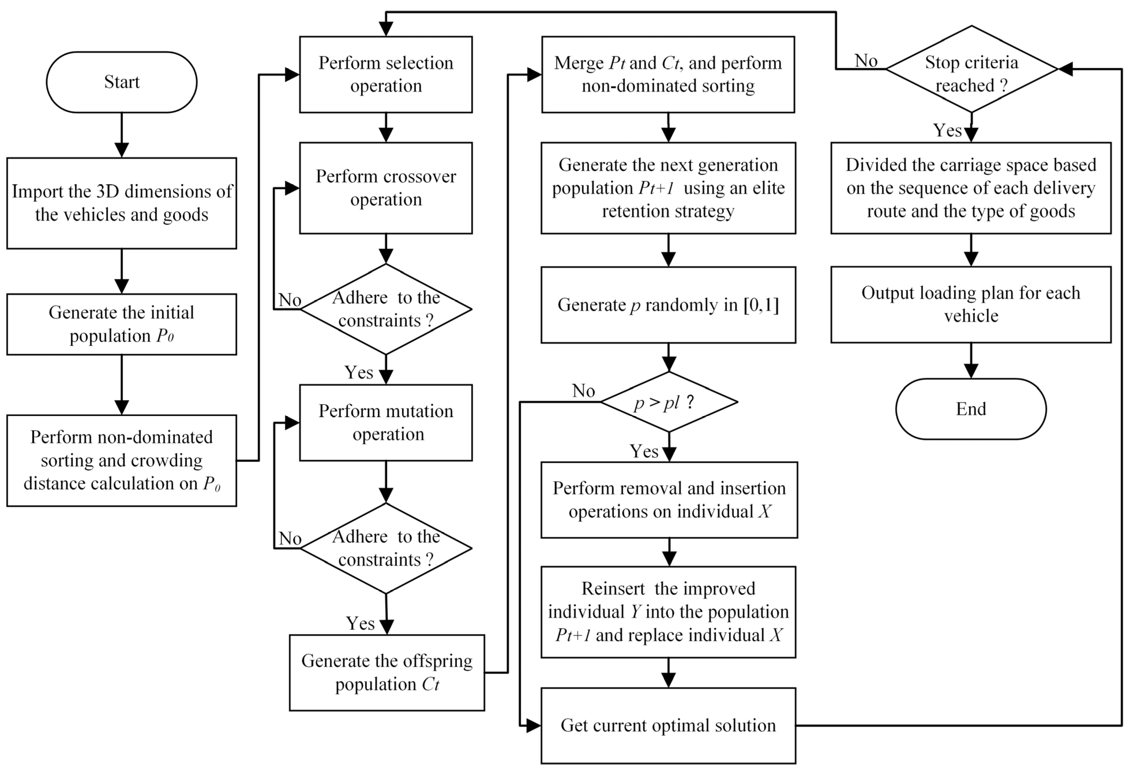
4.1. Main Framework of the Algorithm

The main framework of the MOGA-ALNS is shown in Figure 3. The algorithm’s main structure is derived from genetic algorithms, and ALNS is used to further optimize the route part in each iteration. Finally, the loading plan for goods is determined based on the service sequence of each demand point. Detailed explanations are provided in the subsequent sections.

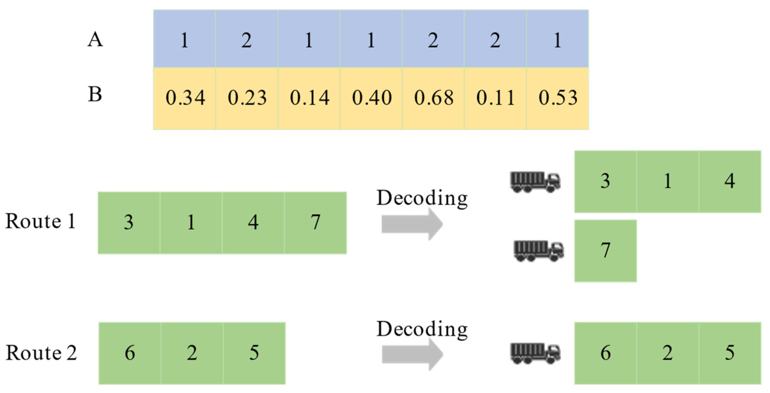
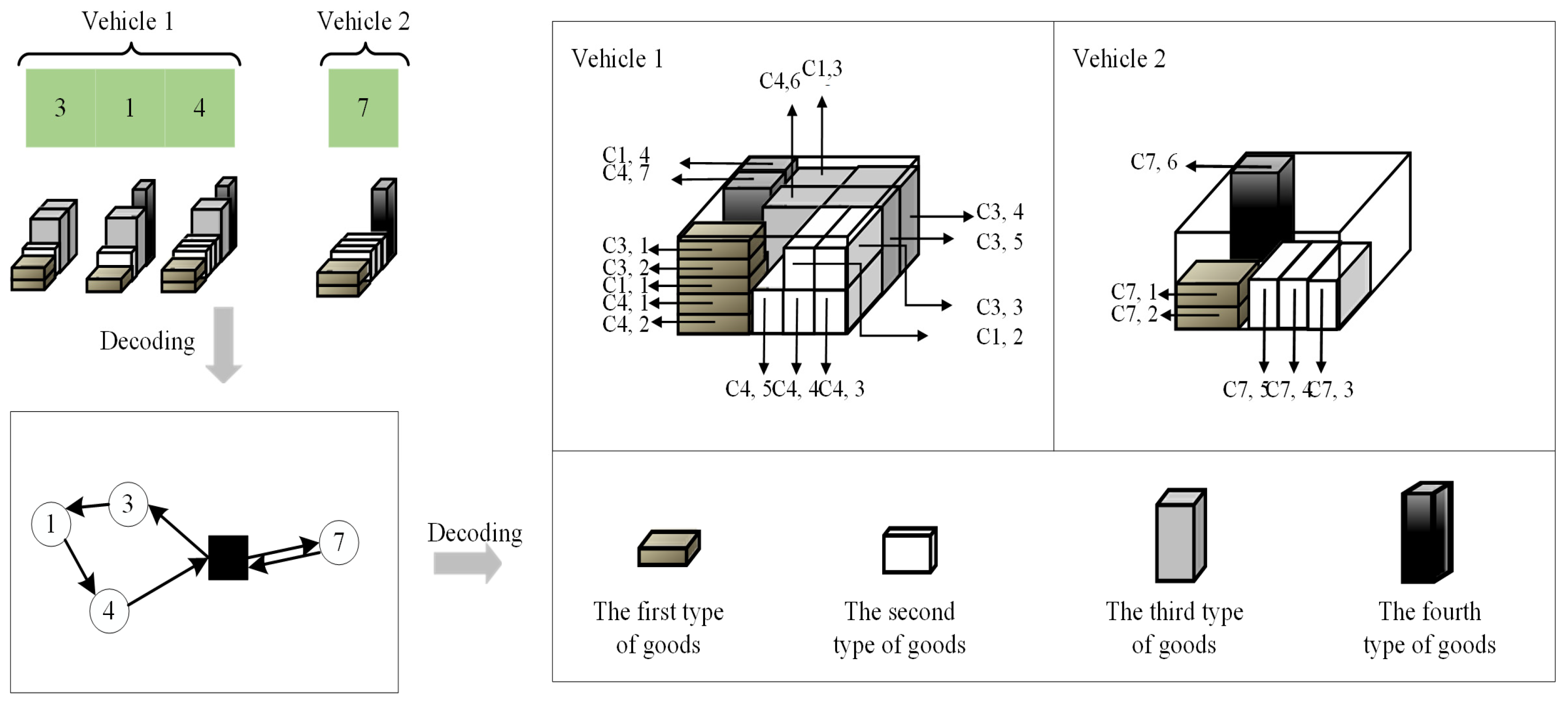
4.2. Representation of Solutions

There are $N$ distribution centers and $M$ demand points. The indices for all distribution centers are integers of 1, 2, …, $N$, and the indices for all demand points are integers of 1, 2, …, $M$. Each solution is represented by a two-dimensional string divided into two parts: A and B. The sequences of the A and B parts correspond one to one, where each position in these sequences represents a specific demand point. This correspondence ensures that the allocation and delivery sequences at each demand point are clearly defined.

The A part, an integer string, indicates each open distribution center and its corresponding demand points. For instance, as shown in Figure 4, Distribution Center 1 serves demand points 1, 3, 4, and 7, while Distribution Center 2 serves 2, 5, and 6. If a distribution center’s total distribution exceeds its capacity but not its maximum expansion limit, it needs expansion. However, exceeding this limit makes the solution’s objective function value extremely large, disqualifying it from further consideration.

The B part consists of floating-point numbers between 0 and 1, assigned randomly to each sequence position. Sorting these numbers in ascending order determines the delivery sequence. This combination of A and B parts clearly indicates the order of deliveries for each distribution center. For example, Figure 4 shows Distribution Center 1 dispatching vehicles to serve demand points in the order of 3-1-4-7, and Center 2 in the order of 6-2-5 to deliver supplies to their respective demand points.

This work adopts vehicle usage rules as shown in Figure 4 to optimize the number of vehicles utilized. The methodology involves sequentially assigning demand points to vehicles for delivery. When a vehicle reaches its maximum capacity, an additional vehicle is allocated for the remaining demand points. Figure 5 elaborates on this process by decoding Route 1 from Figure 4 as a case study. Specifically, Route 1 is bifurcated into two separate delivery paths in accordance with the vehicle usage rules, as depicted in Figure 5. The subsequent phase involves strategically determining the loading sequence of goods, aligning with the established delivery order for each route. This effectively orchestrates the delivery and loading scheme, as visually represented in Figure 5.

4.3. Population Initialization

In this work, $N$ individuals are generated as the initial population to participate in the subsequent optimization process. The method for generating individuals is as follows:

(1)

When considering the distance between demand points and distribution centers, the probability function [60] for assigning all demand points to distribution centers is given by Equation (37), where $d(D_i, C_j)$ represents the Euclidean distance between the distribution center $i$ and demand point $j$, $\overline{d(D, C_j)}$ signifies the average distance from demand point $j$ to all distribution centers, with $n$ representing the total count of demand points. The probability of assigning demand point $j$ to distribution center $i$ is calculated as follows:

$$P\left(D_i,C_j\right)={\displaystyle \frac{max\left\{\overline{d\left(D,C_j\right)}-d\left(D_j,C_j\right),0\right\}}{\sum _{j=1}^{n}max\left\{\overline{d\left(D,C_j\right)}-d\left(D_j,C_j\right),0\right\}}}$$

(37)

According to Equation (37), demand points are more likely to be assigned to the nearest distribution center. At the same time, this method also takes into account the diversity of the initial population, allowing demand points to have the opportunity to be assigned to other centers that are farther away.

(2)

After assigning demand points and distribution centers, we must determine the relationship between vehicles and demand points. In this paper, we use the greedy insertion operator for this initialization, as follows:

Step 1: Arrange all demand points in ascending order of their earliest allowable arrival time within the time window.

Step 2: Iterate through each vehicle to check if the supplies for each demand point can be inserted into that vehicle. This includes checking if there is enough capacity to carry the items in the task. If the quantity of any item in the task, when added to the quantity of supplies already in the vehicle, exceeds the limit, then that vehicle cannot be used for that demand point.

Step 3: For each vehicle, calculate the score (objective function value) of inserting a certain node into it, and record the index of the insertion point, evaluating the effectiveness of different insertion strategies.

Step 4: Among all available vehicles, select the one that results in the lowest insertion score. A lower score indicates that inserting this task contributes least to the growth of the objective function, which means it is a better insertion point.

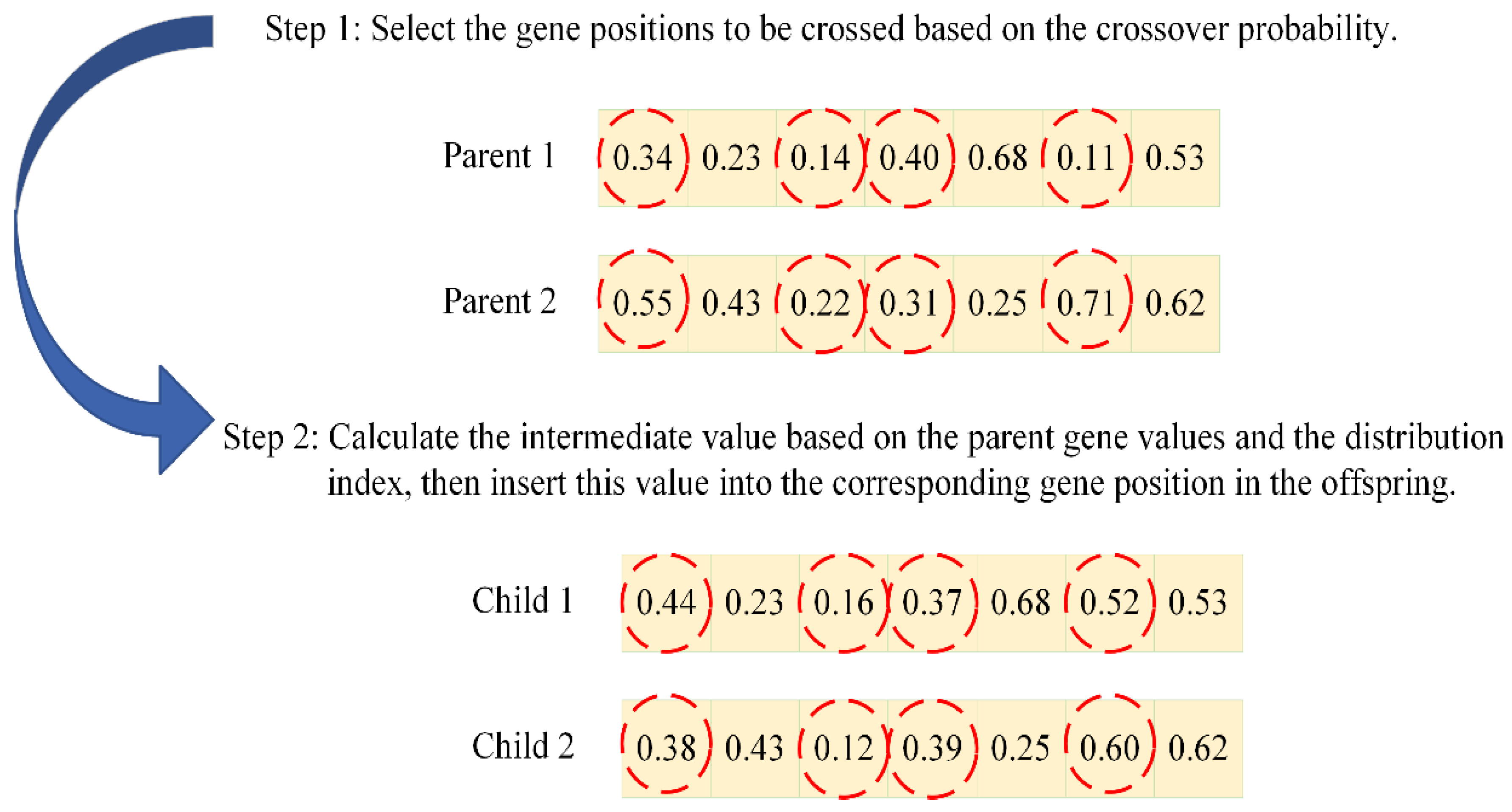
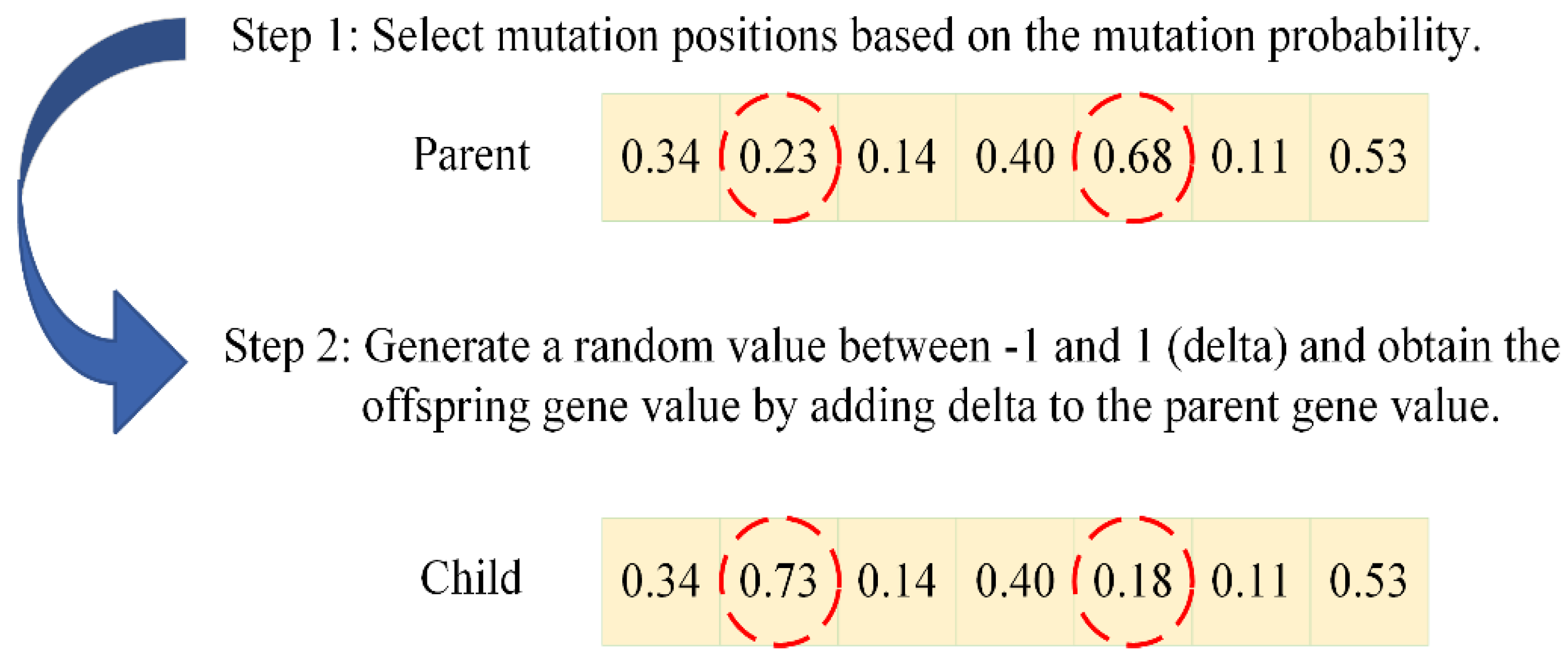
4.4. Selection, Crossover, and Mutation

To enhance the algorithm’s search capability, this study divides the population into multiple clusters using a method based on individual dominance relationships. Individuals at Level 1 that are not dominated are allocated to the first rank of non-dominance, whereas those that are only dominated by individuals at Level 1 receive the second rank of non-dominance, continuing in this manner for subsequent levels. Therefore, all individuals have non-dominated ranks, and individuals with the same rank belong to the same cluster, with the crowding distance of each individual in the cluster subject to calculation. Individuals are grouped based on their rank values, forming clusters. This research proposes specific selection, crossover, and mutation techniques tailored to address the problem described.

In our selection approach, binary tournament selection is utilized when choosing the parent population for crossover and mutation. The detailed procedure is as follows: (1) Two individuals are randomly chosen from the population and evaluated their non-dominated ranks. An individual with the lower rank is selected and preserved. The individual with a greater crowding distance is chosen if both individuals hold identical ranks, and (2) the aforementioned procedures are repeated until the offspring population attains the size of the original population.

The crossover operation in our study generates new solutions by exchanging segments of genetic information among individuals in the population. To enhance diversity and exploration in our evolutionary optimization, we use the simulated binary crossover (SBX) strategy. This operation reassigns and blends the genetic information of two parent solutions, thereby introducing exploratory behavior in the solution space. The detailed process of this crossover is depicted in Figure 6. Additionally, this operator requires the use of two formulas to calculate the values after crossover. Assuming two parent individuals $p^1(x_1^1, \dots ,x_n^1)$ and $p^2(x_1^2, \dots ,x_n^2)$, the two offspring individuals $o^1(x_1^1, \dots ,o_n^1)$ and $o^2(x_1^2, \dots ,o_n^2)$ generated using the SBX operator can be obtained using the following Formula (38):

$$\left\{\begin{array}{c}{y}_i^1=0.5·\left[\left(1+\beta \right)·x_i^1+\left(1-\beta \right)·x_i^2\right]\\ y_i^2=0.5·\left[\left(1-\beta \right)·x_i^1+\left(1+\beta \right)·x_i^2\right]\end{array}\right.$$

(38)

where $\beta$ is determined by the distribution factor $\eta$ according to Formula (39):

$$\beta =\left\{\begin{array}{cc}\hfill {\left(rand·2\right)}^{1/\left(1+\eta \right)}\hfill & rand\le 0.5\hfill \\ \hfill {\left\{1/\left[\left(1-rand\right)·2\right]\right\}}^{1/\left(1+\eta \right)}\hfill & otherwise\hfill \end{array}\right.$$

(39)

Additionally, it should be noted that although chromosome encoding involves both integers and floating-point numbers, both rules are applicable to the above crossover strategy. The only difference is that for integer encoding, after obtaining the intermediate value through the formula, it is necessary to round it to ensure compliance with the encoding rules.

After the crossover operation, the next step is to perform the mutation operation as shown in Figure 7. Each variable for each individual is evaluated. A random number between 0 and 1 is generated and compared with the mutation probability $P_m$. If the generated random number is greater than $P_m$, the original variable is retained. Otherwise, the polynomial mutation strategy is applied for mutation operations. With a probability, each variable in the individual is changed by introducing random perturbation to increase exploration in the solution space. The mutation intensity is controlled by the distribution factor, where larger values result in greater perturbation, increasing individual diversity and helping escape from local optima to enhance global search capability. Similarly, the difference between the mutation in integer encoding and real-number encoding lies in the need to round to integers within the range.

The combination of the above selection, crossover, and mutation strategies drives the population evolution. If the new individuals generated during the crossover and mutation processes do not satisfy the 3D packing constraints, they are replaced, and the same procedure is followed in the subsequent ALNS phase. Ultimately, through this process, a large number of new individuals are generated, and all individuals are merged. The top $N$ best individuals are selected based on non-dominance rank and crowding distance to form a new population.

4.5. Neighborhood Search

In this paper, the neighborhood search is combined with ALNS and the simulated annealing concept. The ALNS framework provides a variety of removal and insertion operators to achieve rapid improvement and convergence of solutions. At the same time, through temperature control and acceptance rules inspired by simulated annealing, the algorithm explores the search space, allowing the acceptance of worse solutions to avoid getting stuck in local optima.

The ALNS can adaptively select the operators with a history of good performance for the next iteration, allowing the operators to fully exploit their search capabilities. This paper designs the following three destruction and two repair operators for the research problem; each operator is assigned a weight and an initial score, and these weights and scores are updated after obtaining a better solution using the operator so that operators with higher scores can be used in subsequent iterations to obtain high-quality solutions.

• Shaw Removal Operator. Calculate the similarity based on the distance between nodes and the required service time, and remove the top $N$ tasks with the highest similarity.
• Random Removal Operator. Randomly remove $n$ task nodes from the vehicle’s delivery route.
• Worst Removal Operator. Remove the $n$ task nodes that result in the largest increase in total cost.
• Greedy Insertion Operator. Sort the task nodes to be inserted in ascending order of their left time windows and insert them to minimize the delivery time as much as possible.
• Regret Insertion Operator. For each unallocated task node, the algorithm calculates the score after inserting it at a certain position, sorts the scores, and selects the top $m$ scores as candidate insertion positions. It computes the sum of the absolute differences between the highest score and the scores of other candidate insertion positions as the regret value for that candidate insertion position. This operator iterates through the list of unallocated tasks, finding the insertion position with the highest regret value for each task.

To escape local optima, this study refers to the acceptance criteria designed by Lin et al. [61]. Suppose $\zeta$ is the initial solution, and ${\mathsf{\zeta }}^{\prime }$ is the new solution obtained following one iteration of ALNS;

Table 2. The neighborhood search introduces five criteria for accepting solutions.

(1) $\Delta f_1\le 0,\Delta f_2\le 0:{\zeta }^{\prime }$ is accepted;

(2) $\Delta f_1\le 0, \Delta f_2>0:{\zeta }^{\prime } \mathrm{i}\mathrm{s} \mathrm{a}\mathrm{c}\mathrm{c}\mathrm{e}\mathrm{p}\mathrm{t}\mathrm{e}\mathrm{d} \mathrm{o}\mathrm{n}\mathrm{l}\mathrm{y} \mathrm{i}\mathrm{f} r<P_1;$

(3) $\Delta f_1>0, \Delta f_2\le 0:{\zeta }^{\prime } \mathrm{i}\mathrm{s} \mathrm{a}\mathrm{c}\mathrm{c}\mathrm{e}\mathrm{p}\mathrm{t}\mathrm{e}\mathrm{d} \mathrm{o}\mathrm{n}\mathrm{l}\mathrm{y} \mathrm{i}\mathrm{f} r<P_2;$

(4) $\Delta f_1>0, \Delta f_2>0 \mathrm{a}\mathrm{n}\mathrm{d} \Delta f_1/f_1\left({\zeta }^{\prime }\right)<\Delta f_2/f_2\left({\zeta }^{\prime }\right):{\mathsf{\zeta }}^{\prime } \mathrm{i}\mathrm{s} \mathrm{a}\mathrm{c}\mathrm{c}\mathrm{e}\mathrm{p}\mathrm{t}\mathrm{e}\mathrm{d} \mathrm{o}\mathrm{n}\mathrm{l}\mathrm{y} \mathrm{i}\mathrm{f} r<P_2;$

(5) $\Delta f_1>0, \Delta f_2>0 \mathrm{a}\mathrm{n}\mathrm{d} \Delta f_1/f_1\left({\zeta }^{\prime }\right)>\Delta f_2/f_2\left({\zeta }^{\prime }\right):{\mathsf{\zeta }}^{\prime } \mathrm{i}\mathrm{s} \mathrm{a}\mathrm{c}\mathrm{c}\mathrm{e}\mathrm{p}\mathrm{t}\mathrm{e}\mathrm{d} \mathrm{o}\mathrm{n}\mathrm{l}\mathrm{y} \mathrm{i}\mathrm{f} r<P_1;$

outlines five criteria for acceptance. Here, $\Delta f_1$ and $\Delta f_2$ denote the differences in objective values between two solutions: $\Delta f_1=f_1\left({\zeta }^{\prime }\right)-f_1\left(\zeta \right)$ and $\Delta f_2=f_2\left({\zeta }^{\prime }\right)-f_2\left(\zeta \right)$. Additionally, we need $P_1$, $P_2$, and $r$, where $P_1=\mathit{exp}\left(-\Delta f_1∕K·T\right)$, $P_2=\mathit{exp}\left(-\Delta f_2∕K·T\right)$; $r$ is a random number uniformly distributed in [0, 1], $T$ is the temperature coefficient, and the Boltzmann constant $K=1$.

During every iteration, the probability $pl$ governs the refinement of each solution $X$ through the neighborhood search process. It is important to note that there are three distinct instances of $X$ in this context: $X$ refers to the current solution, $X^t$ refers to the current solution $X$ after the removal and insertion operations, and $X^b$ refers to the best historical solution up to the current point. Furthermore, the score for solution $X$ is denoted as $G\left(X\right)$, where $Rem\left(X\right)$ represents the removal operation applied to solution $X$, and $Ins\left(X\right)$ represents the insertion operation applied to solution $X$. ${\rho }^{-}$ represents the probability of choosing different removal operators, while ${\rho }^{+}$ represents the probability of selecting different insertion operators. Initially, both ${\rho }^{-}$ and ${\rho }^{+}$ are set to 1, meaning all operators have an equal chance of being selected. After each iteration, these probabilities are updated. ${\theta }^{-}$ denotes the set of removal operators, and ${\theta }^{+}$ denotes the set of insertion operators. The current choice of removal and insertion operators for each iteration is determined using a roulette wheel selection method. In this method, the probability of selection is directly proportional to the values of ${\rho }^{-}$ and ${\rho }^{+}$, meaning higher values for ${\rho }^{-}$ and ${\rho }^{+}$ result in a greater likelihood of being chosen. The procedure of the neighborhood search is provided by Algorithm 1.

Algorithm 1. Procedure of the Neighborhood Search
1:	input: a feasible solution $X$
2:	$X^b=X$; ${\rho }^{-}=\left(1,\dots ,1\right)$; ${\rho }^{+}=\left(1,\dots ,1\right)$;
3:	repeat
4:	select removal and insertion operations $Rem \in {\theta }^{-}$ and $Ins\in$
5:	${\theta }^{-}$ using ${\rho }^{-}$ and ${\rho }^{+}$;
6:	$X^t=Ins\left(Rem\left(X\right)\right)$;
7:	if (any of five conditions is satisfied) then
8:	$X=X^t;$
9:	end if
10:	if $G\left(X^t\right)$ < $G\left(X^b\right)$  then
11:	$X^b=X^t;$
12:	end if
13:	update ${\rho }^{-}$ and ${\rho }^{+}$;
14:	until stop criterion is met
15:	return $X^b$

5. Numerical Experiments

Given the lack of consideration for our researched problem in existing studies, the corresponding algorithms in the literature cannot be directly employed to solve the problem under investigation. Therefore, this work chooses the strength pareto evolutionary algorithm II (SPEA-II) [62], multi-objective evolutionary algorithm based on decomposition (MOEA/D) [63], and multi-objective evolutionary algorithm based on decomposition with dynamic resource allocation (MOEA/D-DRA) [64] as comparative algorithms. The SPEA-II and MOEA/D are classic multi-objective evolutionary algorithms and have received positive evaluations in vehicle routing problems [65,66,67,68]. The MOEA/D-DRA is a variant of the MOEA/D, introducing a dynamic resource allocation strategy to make more efficient use of computational resources and enhance the performance and efficiency of the algorithm [69]. In this paper, we compare our proposed algorithm to these three. Details on the SPEA-II, MOEA/D, and MOEA/D-DRA are as follows:

(1)

SPEA-II adopts the solution representation method similar to the MOGA-ALNS, as detailed in Section 4.2. It begins with the generation of a random population using the method described in the same section. The selection and population update mechanisms adhere to the foundational structure of the SPEA-II, as outlined in the literature [62]. For genetic operations, SPEA-II incorporates the same crossover and mutation techniques as found in the MOGA-ALNS, ensuring consistency in the approach to evolving solutions.

(2)

Aligning with the MOGA-ALNS for solution representation, the MOEA/D leverages the Tchebycheff approach to create a series of subproblems targeting different parts of the objective space [63]. The processes for constructing neighborhoods, selecting individuals, and updating individual solutions are all based on the core principles of the MOEA/D [63]. Furthermore, the algorithm applies identical crossover and mutation strategies as the MOGA-ALNS, facilitating a uniform method of introducing genetic diversity and exploring the solution space.

The MOEA/D-DRA not only aligns with the MOGA-ALNS in terms of solution representation but also in the employment of the Tchebycheff approach for formulating single-objective subproblems. The method for building neighborhoods and the protocols for individual selection and updates are in line with the MOEA/D-DRA framework [64]. Like the other algorithms, the MOEA/D-DRA utilizes the same crossover and mutation operations as the MOGA-ALNS, ensuring a coherent approach to optimization across different methodologies.

5.1. Test Case

In this paper, we made appropriate modifications to the classic instances proposed by Cordeau to accommodate the characteristics of our problem and designed the test case set used in the following sections, which consists of 20 instances. We considered five different scenarios. Specifically, the first scenario represents a situation where none of the candidate distribution centers experience disruptions. In the other scenarios, one or two distribution centers encounter disruptions. These instances are distinguished by the named form $\left|I\right|-\left|J\right|-\mathrm{a}$, where $\left|I\right|$ is the number of candidate distribution centers, $\left|J\right|$ is the number of demand points, a represents the first scenario, and b, c, d, and e represent the other four scenarios.

Four different types of commodities were selected, and the demand quantity of each commodity for each customer is randomly generated in the range of [10, 20]. Penalty coefficients for early and late arrivals are randomly generated from the range [1, 3], transportation costs per unit time are randomly generated from the range [5, 10], vehicle transportation speeds are randomly generated in the range [5, 10], distribution center location costs are randomly generated from the range [100, 200], unit expansion costs are randomly generated from the range [10, 20], and the probabilities of secondary disasters occurring at individual distribution centers and road segments, as well as the probability of significant damage caused by disasters, are randomly generated in the range (0, 0.5]. The capacity ${\beta }_i$ of each distribution center is determined using the following method: we first calculate the average required capacity $\overline{\beta }$ using the following Formula (40):

$$\overline{\beta }={\displaystyle \frac{d}{\left|I\right|}}$$

(40)

where $d$ represents the total capacity of the materials required at the point of demand, and $\left|I\right|$ represents the number of candidate distribution centers. Then, the capacity of each distribution center ${\beta }_i$ is randomly generated at $\left[1.5\overline{\beta }, 2\overline{\beta }\right]$.

5.2. Performance Metrics

The aim of the MOGA-ALNS is to discover a set of solutions that exhibit both good convergence and diversity. Consequently, to better assess the approximation and distribution of the obtained solution set, this study utilizes C-metric [70], IGD-metric [71], and hypervolume-metric [72] as evaluation indicators. Moreover, we employ the t-test to analyze the significance of the results obtained using the MOGA-ALNS, SPEA-II, MOEA/D, and MOEA/D-DRA. When the MOGA-ALNS is significantly better, significantly worse, or statistically equivalent to other algorithms, the results are indicated as “$+$”, “$-$”, or “$~$”.

(1)

The C-metric, a tool for evaluating the comparative performance of two different algorithms through their solution sets $X$ and $Y$, quantifies the extent to which one set dominates another. Specifically, $C(X, Y)$ represents the proportion of solutions in set $Y$ that are dominated by at least one solution in set $X$. The formula for calculating this metric is as follows:

$$C\left(X,Y\right)={\displaystyle \frac{\left|\left\{yϵ\left.Y\right|\exists xϵX:x\prec y\right\}\right|}{\left|Y\right|}}$$

(41)

(2)

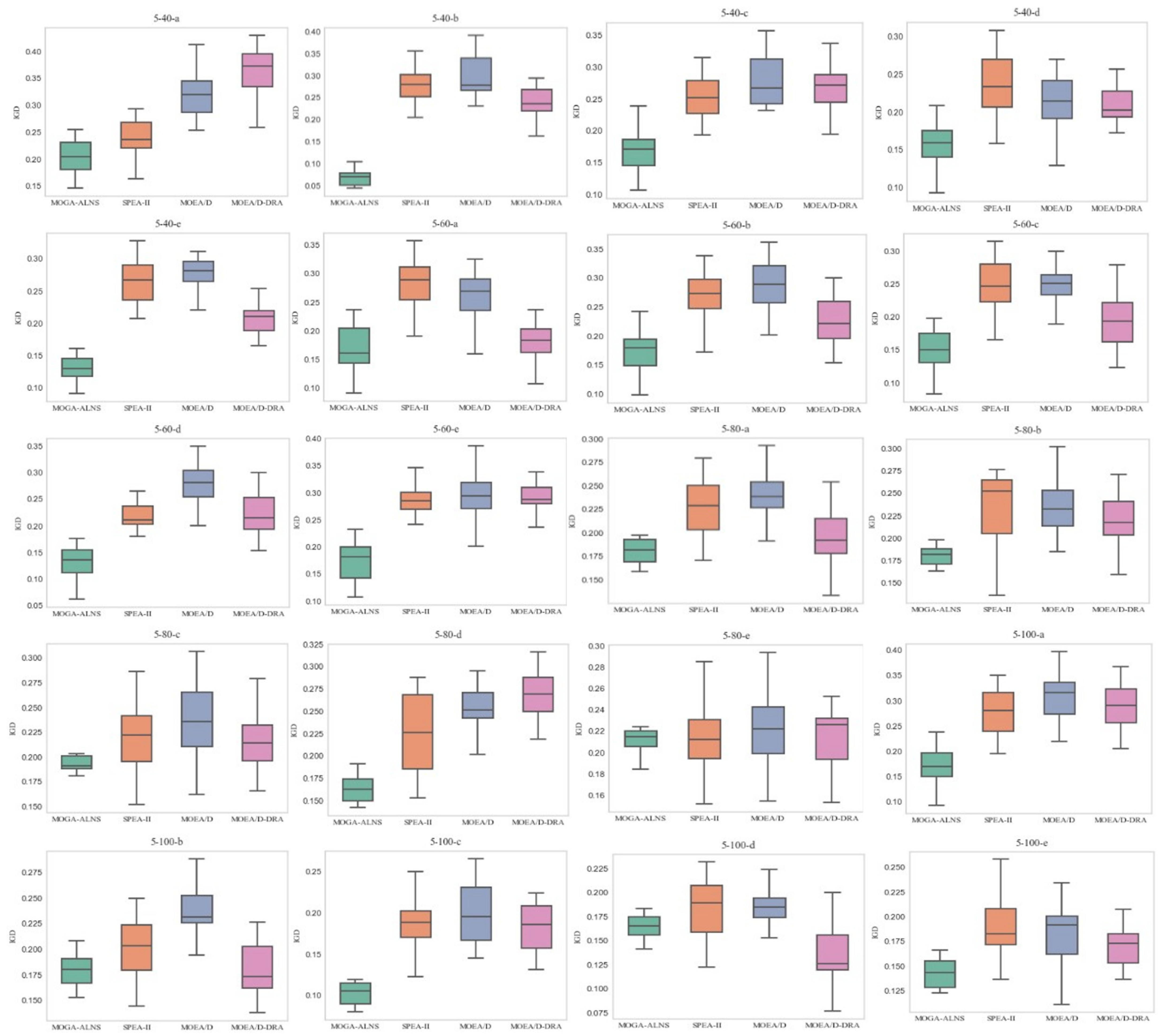
The IGD-metric calculates the minimum Euclidean distance between the approximate solution set and the Pareto-optimal front. A smaller IGD value indicates that the solution set generated by the algorithm is closer to the true front. Let $Z^{*}$ and $Z$ represent the optimal solution set and the approximate solution set, respectively. Formula (41) for IGD measurement is as follows:

$$IGD\left(Z, Z^{*}\right)={\displaystyle \frac{1}{\left|Z^{*}\right|}}\sum _{z\in Z^{*}}dist\left(z,Z\right)$$

(42)

where $dist\left(z, Z\right)$ is the Euclidean distance between a solution $z$ in $Z^{*}$ and the closest solution to it in $Z$. Therefore, in the calculation of IGD, it is first necessary to have a known true front or an ideal front that represents the best solutions to the problem. Since the Pareto-optimal front of the studied problem is unknown, this study combines all non-dominated solutions obtained by various methods and considers them as an approximate Pareto-optimal front. Furthermore, this study normalizes all objective values, mapping them into the range [0, 1] before calculating the IGD.

(3)

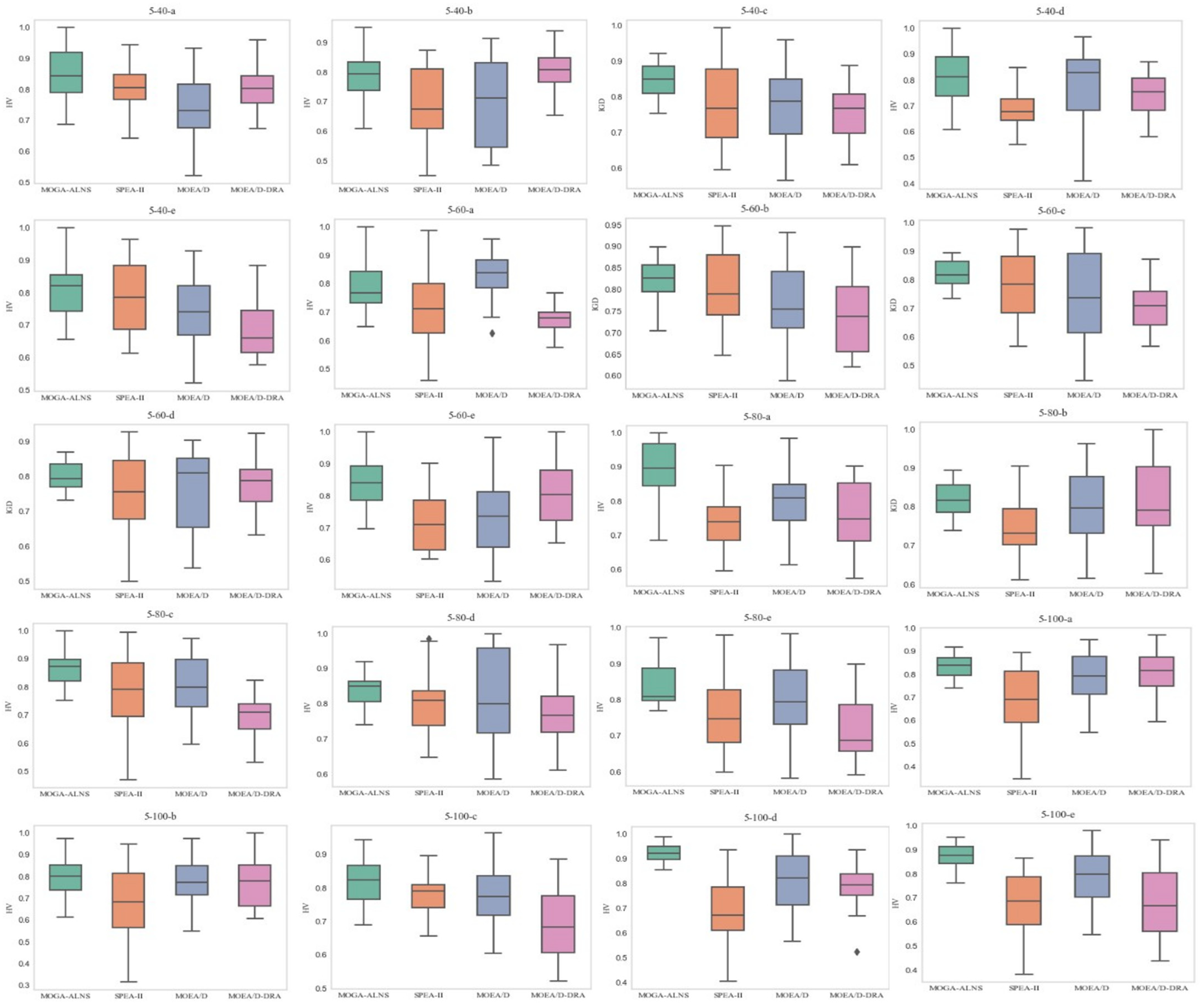
The hypervolume-metric measures the coverage range size of the approximate set in the objective space. A higher hypervolume value indicates a broader coverage range of the approximate set in the objective space, which typically implies the higher quality of the obtained non-dominated solution set. Let $y^{*}=(y_1^{*}, y_2^{*})$ be the reference point in the objective space dominated by all optimal solutions. Then, the hypervolume value of the solution set represents the volume of a region where all solutions are dominated by the solution set and dominate $y^{*}$. When calculating the hypervolume-metric, a reference point needs to be selected. In this paper, (1, 1) is used as the reference point, and all objective values in the approximate solution set are normalized, mapping them into the range [0, 1].

5.3. Parameter Configuration

To investigate the impact of algorithm parameter settings on the performance of the MOGA-ALNS, we employed an orthogonal experiment to explore the optimal parameter combinations, including population size $N$, simulated annealing rate $\alpha$, and the number of iterations without improvement $\theta$. We defined four levels for each of the three parameters: $N \in \{50, 75, 100, 125\}$, $\alpha \in \{0.3, 0.5, 0.7, 0.9\}$, and $\theta \in \{30, 60, 90, 120\}$. Consequently, we constructed an orthogonal array ${\mathrm{L}}_{16}\left(4^3\right)$ with 16 parameter combinations, as shown in

Table 3. Orthogonal table and experimental results.

No	$\mathit{N}$	$\mathit{\alpha }$	$\mathit{\theta }$	ARV
1	50	0.3	30	0.7555
2	50	0.5	60	0.7659
3	50	0.7	90	0.8319
4	50	0.9	120	0.8440
5	75	0.3	60	0.8035
6	75	0.5	30	0.8853
7	75	0.7	120	0.8059
8	75	0.9	90	0.9506
9	100	0.3	90	0.9447
10	100	0.5	120	0.8874
11	100	0.7	30	0.8825
12	100	0.9	60	0.8303
13	125	0.3	120	0.8796
14	125	0.5	90	0.9341
15	125	0.7	60	0.8624
16	125	0.9	30	0.9682

.

In this experiment, we selected the hypervolume-metric as the response value (RV) and independently ran each parameter combination 20 times, calculating the average RV value based on the results of 20 independent runs. The results of the orthogonal experiment are shown in Table 3, and the significance ranking of parameters is shown in

Table 4. Influence trend and rank.

Level	$\mathit{N}$	$\mathit{\alpha }$	$\mathit{\theta }$
1	0.7993	0.8458	0.8729
2	0.8613	0.8682	0.8155
3	0.8862	0.8456	0.9153
4	0.9111	0.8983	0.8542
Delta	0.1117	0.0526	0.0998
Rank	1	3	2

. Furthermore, Figure 8 depicts the trends in parameter influence. Based on the results from Table 4 and Figure 8, we can observe that the population size $N$ plays the most crucial role in the MOGA-ALNS, followed by the number of iterations without improvement $\theta$ ranking second, and the simulated annealing rate $\alpha$ ranking third. Therefore, this study concludes, through an analysis of the experimental results, that the MOGA-ALNS performs best when $N$ = 125, $\alpha$ = 0.9, and $\theta$ = 90.

5.4. Effectiveness of Neighborhood Search

In the MOGA-ALNS, ALNS is utilized as a neighborhood search mechanism to further improve the solutions for path optimization. To assess the contributions of neighborhood search within the MOGA-ALNS framework, we developed a modified version that operates without the neighborhood search component, referred to as MOGA-ALNS-w/o-NS. Subsequently, we processed all instances using both MOGA-ALNS and MOGA-ALNS-w/o-NS, evaluating their experimental outcomes through the hypervolume-metric and IGD-metric, as presented in

Table 5. Experimental results for the MOGA-ALNS and MOGA-ALNS-w/o-NS based on the hypervolume-metric and IGD-metric.

Instance	Hypervolume-Metric						IGD-Metric
	MOGA-ALNS			MOGA-ALNS-w/o-NS			MOGA-ALNS			MOGA-ALNS-w/o-NS
	Mean	Var	Rank	Mean	Var	Rank	Mean	Var	Rank	Mean	Var	Rank
5-40-a	0.8442	0.0083	1	0.7442	0.0161	2	0.2064	0.0015	1	0.2679	0.0016	2
5-40-b	0.7867	0.0101	1	0.7589	0.0108	2	0.0726	0.0005	1	0.2746	0.0009	2
5-40-c	0.8359	0.0104	1	0.7537	0.0105	2	0.1721	0.0011	1	0.2642	0.0014	2
5-40-d	0.8119	0.0131	1	0.7894	0.0086	2	0.1621	0.0017	1	0.2222	0.0018	2
5-40-e	0.8217	0.0097	1	0.7670	0.0093	2	0.1329	0.0005	1	0.2541	0.0013	2
5-60-a	0.7867	0.0106	2	0.7936	0.0103	1	0.1708	0.0018	1	0.2468	0.0022	2
5-60-b	0.7986	0.0182	1	0.7274	0.0203	2	0.1739	0.0013	1	0.2630	0.0016	2
5-60-c	0.8148	0.0190	1	0.7952	0.0152	2	0.1500	0.0009	1	0.2173	0.0014	2
5-60-d	0.7829	0.0180	1	0.7577	0.0153	2	0.1308	0.0008	1	0.2500	0.0014	2
5-60-e	0.8466	0.0060	1	0.7323	0.0146	2	0.1713	0.0013	1	0.2790	0.0023	2
5-80-a	0.8939	0.0089	1	0.7733	0.0140	2	0.1714	0.0022	1	0.2062	0.0012	2
5-80-b	0.8251	0.0148	1	0.7641	0.0195	2	0.1803	0.0016	1	0.2119	0.0011	2
5-80-c	0.8641	0.0043	1	0.7670	0.0184	2	0.1966	0.0009	1	0.2035	0.0013	2
5-80-d	0.8354	0.0030	1	0.7626	0.0076	2	0.1580	0.0017	1	0.2647	0.0015	2
5-80-e	0.8456	0.0043	1	0.7557	0.0125	2	0.2485	0.0027	2	0.2094	0.0013	1
5-100-a	0.8317	0.0024	1	0.7618	0.0104	2	0.1700	0.0016	1	0.3164	0.0010	2
5-100-b	0.7985	0.0098	1	0.7070	0.0054	2	0.1795	0.0007	1	0.2278	0.0010	2
5-100-c	0.8173	0.0056	1	0.8095	0.0154	2	0.0988	0.0007	1	0.1916	0.0010	2
5-100-d	0.9211	0.0015	1	0.7455	0.0178	2	0.1797	0.0007	2	0.1587	0.0013	1
5-100-e	0.8750	0.0024	1	0.7647	0.0105	2	0.1401	0.0007	1	0.1633	0.0006	2
Average	0.8319	0.0090	1.0500	0.7605	0.0131	1.9500	0.1632	0.0012	1.1000	0.2346	0.0013	1.9000

(where “var” denotes variance). Among the 20 instances, the MOGA-ALNS algorithm outperformed MOGA-ALNS-w/o-NS in 18 instances, as evidenced by its higher mean hypervolume-metric values, thus underscoring the effectiveness of incorporating neighborhood search in enhancing algorithmic performance.

By computing the average means and variances in the hypervolume-metric from 20 independent trials, the resultant average Hypervolume values for the MOGA-ALNS and MOGA-ALNS-w/o-NS are 0.8319 and 0.7605, respectively. The corresponding variances for these averages are 0.0090 for the MOGA-ALNS and 0.0131 for MOGA-ALNS-w/o-NS. This indicates that the MOGA-ALNS outperforms MOGA-ALNS-w/o-NS, as it achieves a higher average value relative to the mean. This superiority suggests that the inclusion of local search contributes significantly to performance, reflecting its ability to find more effective solutions by exploiting the search space more efficiently.

By averaging the means of the IGD-metric across 20 runs, the average values for the MOGA-ALNS and MOGA-ALNS-w/o-NS with respect to the mean are found to be 0.2334 and 0.2646, respectively, and with respect to variance, the average values are 0.0012 and 0.0013, respectively. This indicates that the MOGA-ALNS outperforms MOGA-ALNS-w/o-NS, as it achieves lower average values in terms of both mean and variance. The lower average values for the MOGA-ALNS reflect its superior performance, demonstrating its efficiency in producing solutions that are nearer to the true Pareto front and with less variability between runs, thus underlining the effectiveness of integrating neighborhood search strategies within the MOGA-ALNS framework for optimizing solutions.

To rigorously evaluate and compare the performance differences between the MOGA-ALNS and MOGA-ALNS-w/o-NS, this study employs statistical testing methods, specifically the Friedman test [73] and the Nemenyi post-hoc test [74]. These tests are instrumental in identifying statistically significant differences in the algorithms’ performances across multiple datasets or problem instances.

(1)

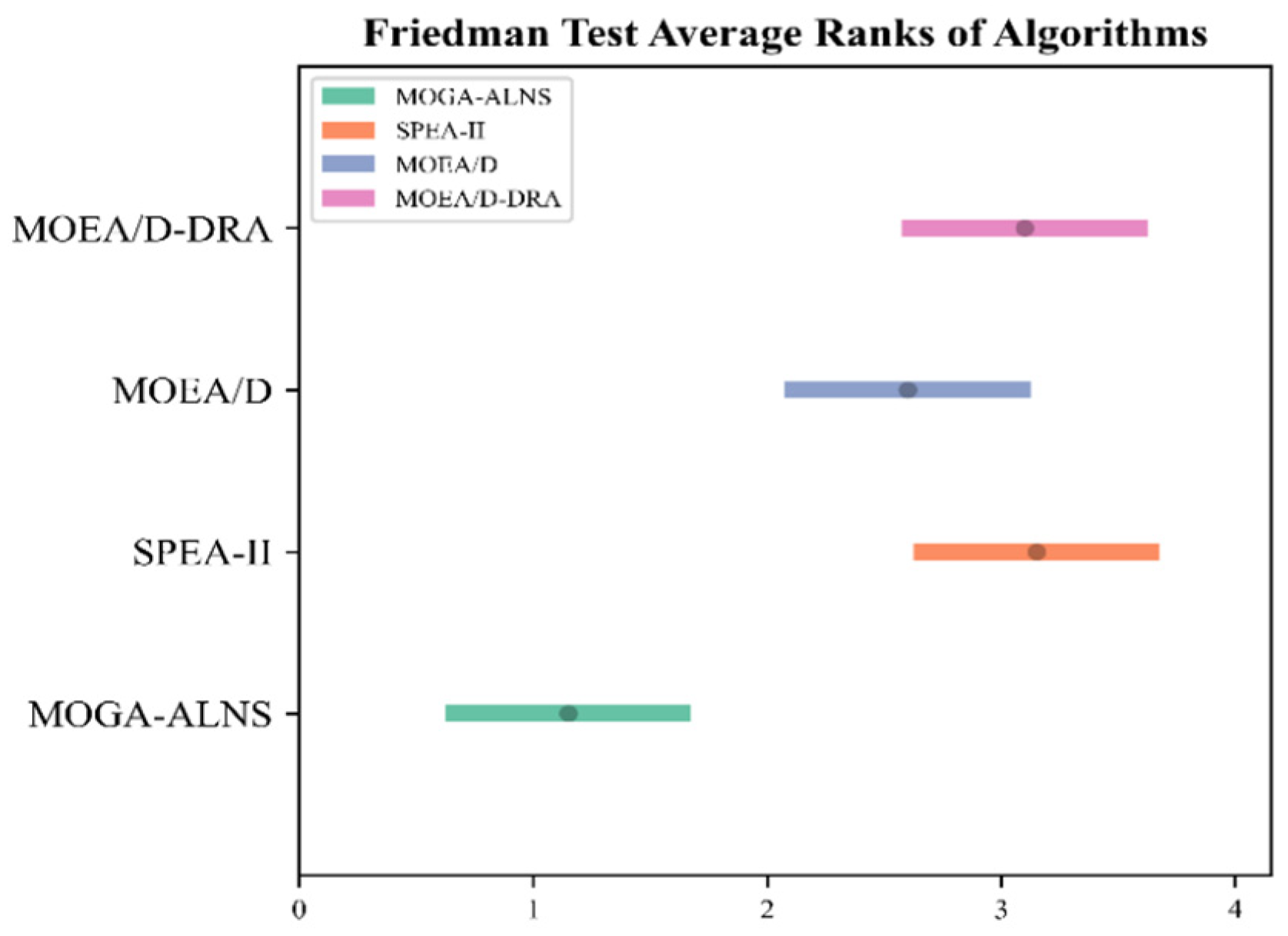
In the Friedman test, we organize the MOGA-ALNS and MOGA-ALNS-w/o-NS by descending average values of the hypervolume-metric and ascending average values for the IGD-metric, assigning them ranks of 1 and 2, respectively. We then calculate the average ranks across all instances as depicted in Table 5. For the hypervolume-metric, the average ranks are 1.05 for the MOGA-ALNS and 1.95 for MOGA-ALNS-w/o-NS. Similarly, for the IGD-metric, the average ranks stand at 1.1000 for the MOGA-ALNS and 1.9000 for MOGA-ALNS-w/o-NS. This differentiation in average ranks allows us to deduce a statistically significant disparity in performance between the MOGA-ALNS and MOGA-ALNS-w/o-NS according to the Friedman test.

(2)

To delve deeper into the distinctions between the MOGA-ALNS and MOGA-ALNS-w/o-NS, we employ the Nemenyi post-hoc test at a significance level of 0.05 to ascertain the critical discrepancy in their average rank values. The gap in average ranks for the hypervolume-metric is 0.9000, surpassing the critical threshold of 0.4382. Similarly, for the IGD metric, the difference in average ranks is 0.8000, also exceeding the critical value. These findings underscore the MOGA-ALNS’s notable superiority over MOGA-ALNS-w/o-NS across both evaluated metrics.

The results indicate that the neighborhood search indeed enhances the search capabilities of the MOGA-ALNS, playing a positive role in the search process. This demonstrates the effectiveness of integrating neighborhood search strategies into the MOGA-ALNS framework, leading to improved performance in solving optimization problems by facilitating a more thorough exploration of the solution space.

5.5. Experimental Results

This section provides a comprehensive comparison of the MOGA-ALNS, SPEA-II, MOEA/D, and MOEA/D-DRA. The parameter settings for the experiments are as follows [68,75]. For SPEA-II, the population size is set to 100, with a crossover probability of 0.7 and a mutation probability of 0.3. MOEA/D has a population size of 100, a crossover probability of 0.8, a mutation probability set to 1, and a neighborhood size set to 20. The parameter settings for the MOEA/D-DRA are from the literature [64], which include a population size of 600, a crossover probability of 0.8, a mutation probability of 0.2, and a neighborhood size of 20.

5.5.1. Analysis of the C-Metric

Table 6. C-metric comparison of the four approaches.

Instance	C (GA, EAD)	C (EAD, GA)	t-Test	C (GA, SPEA)	C (SPEA, GA)	t-Test	C (GA, DRA)	C (DRA, GA)	t-Test
5-40-a	0.7589	0.0807	$+$	0.7267	0.0863	$+$	0.5183	0.0923	$+$
5-40-b	0.8063	0.0208	$+$	0.8110	0.0513	$+$	0.7292	0.0618	$+$
5-40-c	0.8481	0.0310	$+$	0.6696	0.0575	$+$	0.6801	0.0836	$+$
5-40-d	0.7870	0.0518	$+$	0.8489	0.0499	$+$	0.6589	0.0731	$+$
5-40-e	0.8945	0.0146	$+$	0.8588	0.0208	$+$	0.7427	0.0427	$+$
5-60-a	0.7667	0.0458	$+$	0.7828	0.0739	$+$	0.2857	0.1631	$+$
5-60-b	0.7624	0.0000	$+$	0.7983	0.0405	$+$	0.6721	0.1010	$+$
5-60-c	0.8135	0.0467	$+$	0.8265	0.0351	$+$	0.6653	0.0494	$+$
5-60-d	0.8787	0.0000	$+$	0.8546	0.0310	$+$	0.6967	0.1147	$+$
5-60-e	0.8237	0.0208	$+$	0.8574	0.0296	$+$	0.5813	0.1120	$+$
5-80-a	0.6475	0.0143	$+$	0.6276	0.0482	$+$	0.4677	0.0488	$+$
5-80-b	0.6470	0.0250	$+$	0.8523	0.0350	$+$	0.4133	0.0417	$+$
5-80-c	0.8275	0.0333	$+$	0.7361	0.0393	$+$	0.6665	0.0714	$+$
5-80-d	0.8558	0.0458	$+$	0.6980	0.1244	$+$	0.7835	0.0796	$+$
5-80-e	0.7614	0.0125	$+$	0.8023	0.0000	$+$	0.6322	0.0333	$+$
5-100-a	0.9483	0.0083	$+$	0.9217	0.0167	$+$	0.7924	0.0917	$+$
5-100-b	0.7964	0.0283	$+$	0.7343	0.0767	$+$	0.5742	0.1233	$+$
5-100-c	0.5983	0.0444	$+$	0.7663	0.1409	$+$	0.6745	0.1937	$+$
5-100-d	0.8598	0.0100	$+$	0.7638	0.0267	$+$	0.4888	0.1600	$+$
Average	0.7902	0.0284	$+$	0.7848	0.0495	$+$	0.5218	0.0429	$+$

presents the outcomes of the C-metric analysis, with the acronyms “GA”, “EAD”, “SPEA”, and “DRA” denoting the MOGA-ALNS, SPEA-II, MOEA/D, and MOEA/D-DRA, respectively. For each instance, the average value calculated using the C-metric over 20 runs is presented. Furthermore, to ensure a clear analysis of the experimental outcomes, we employ a one-tailed t-test with 38 degrees of freedom and a 0.05 significance level [70] to verify the differences between MOGA-ALNS and its competitors. Table 6 illustrates the performance comparison using the symbols “$+$”, “$-$”, and “$~$” to indicate scenarios where the MOGA-ALNS is significantly superior, significantly inferior, or statistically on par with the compared algorithms, respectively.

In comparing the MOGA-ALNS to the SPEA-II, it is evident that the MOGA-ALNS yields better results than the SPEA-II, as the solutions obtained using the MOGA-ALNS are all superior to those obtained using the SPEA-II. Conversely, since the C (SPEA, GA) values are all less than C (GA, SPEA) in 20 instances, it indicates that the solutions obtained using the SPEA-II are not superior to those found using the MOGA-ALNS. Similarly, in comparing the MOGA-ALNS to the MOEA/D, it is observed that in all 20 instances, the solutions obtained using the MOGA-ALNS are superior to those obtained using the MOEA/D. In contrast, with all instances showing C (EAD, GA) values less than C (GA, EAD), the solutions obtained using the MOEA/D are not superior to those found by the MOGA-ALNS. Similarly, by comparing the MOGA-ALNS to the MOEA/D-DRA, it can be inferred that the MOGA-ALNS achieves better outcomes than the MOEA/D-DRA, as the majority of solutions obtained using the MOGA-ALNS in all 20 instances are superior to those found using the MOEA/D-DRA. Based on the above analysis, we can conclude that the MOGA-ALNS exhibits a better ability to find more non-dominated solutions and demonstrates superior performance in solving related problems compared to SPEA-II, MOEA/D, and MOEA/D-DRA.

5.5.2. Analysis of the IGD-Metric

The IGD-metric results obtained from the experiments comparing the MOGA-ALNS to the other algorithms are presented in

Table 7. Experimental results obtained using the IGD-metric.

Instance	MOGA-ALNS		SPEA-II			MOEA/D			MOEA/D-DRA
	Mean	Var	Mean	Var	t-Test	Mean	Var	t-Test	Mean	Var	t-Test
5-40-a	0.2065	0.0030	0.2411	0.0011	$+$	0.3199	0.0019	$+$	0.3630	0.0022	$+$
5-40-b	0.0697	0.0003	0.2794	0.0016	$+$	0.2995	0.0024	$+$	0.2411	0.0011	$+$
5-40-c	0.1722	0.0012	0.2538	0.0014	$+$	0.2764	0.0015	$+$	0.2674	0.0011	$+$
5-40-d	0.1572	0.0008	0.2361	0.0020	$+$	0.2110	0.0016	$+$	0.2097	0.0006	$+$
5-40-e	0.1315	0.0004	0.2647	0.0014	$+$	0.2763	0.0007	$+$	0.2065	0.0005	$+$
5-60-a	0.1708	0.0018	0.2783	0.0017	$+$	0.2598	0.0020	$+$	0.1805	0.0009	$~$
5-60-b	0.1740	0.0013	0.2698	0.0016	$+$	0.2881	0.0019	$+$	0.2234	0.0022	$+$
5-60-c	0.1501	0.0009	0.2499	0.0014	$+$	0.2499	0.0009	$+$	0.1951	0.0015	$+$
5-60-d	0.1309	0.0009	0.2195	0.0006	$+$	0.2787	0.0013	$+$	0.2235	0.0018	$+$
5-60-e	0.1714	0.0013	0.2898	0.0009	$+$	0.2954	0.0017	$+$	0.2907	0.0009	$+$
5-80-a	0.1799	0.0002	0.2267	0.0011	$+$	0.2392	0.0007	$+$	0.1949	0.0011	$+$
5-80-b	0.1808	0.0001	0.2345	0.0015	$+$	0.2353	0.0011	$+$	0.2204	0.0009	$+$
5-80-c	0.1938	0.0001	0.2180	0.0017	$+$	0.2328	0.0016	$+$	0.2175	0.0010	$+$
5-80-d	0.1642	0.0002	0.2260	0.0021	$+$	0.2528	0.0007	$+$	0.2670	0.0008	$+$
5-80-e	0.2110	0.0002	0.2102	0.0012	$~$	0.2255	0.0013	$+$	0.2129	0.0008	$~$
5-100-a	0.1658	0.0019	0.2771	0.0019	$+$	0.3093	0.0026	$+$	0.2875	0.0021	$+$
5-100-b	0.1806	0.0003	0.2027	0.0008	$+$	0.2371	0.0007	$+$	0.1808	0.0007	$~$
5-100-c	0.1023	0.0002	0.1886	0.0012	$+$	0.2019	0.0014	$+$	0.1830	0.0008	$+$
5-100-d	0.1649	0.0002	0.1840	0.0010	$+$	0.1856	0.0003	$+$	0.1356	0.0008	$-$
5-100-e	0.1434	0.0002	0.1929	0.0011	$+$	0.1814	0.0010	$+$	0.1717	0.0005	$+$
Average	0.1610	0.0008	0.2372	0.0014	$+$	0.2528	0.0014	$+$	0.2236	0.0011	$+$

. The MOGA-ALNS demonstrates superior performance over the MOEA/D in every instance, evidenced by the lower mean and variance in IGD-metric values for the MOGA-ALNS compared to the MOEA/D, after conducting 20 trials per instance. Furthermore, the MOGA-ALNS is superior to both the SPEA-II and MOEA/D-DRA in 19 out of 20 instances, as indicated by the lower average IGD-metric values of the MOGA-ALNS compared to those of the SPEA-II and MOEA/D-DRA. More specifically, t-test results show that the MOGA-ALNS performs significantly better than the SPEA-II in 19 of 20 instances and significantly better than the MOEA/D-DRA in 16 of 20 instances.

By averaging the means and variances of the 20 runs, as shown in Table 7, the average mean values for the MOGA-ALNS, SPEA-II, MOEA/D, and MOEA/D-DRA are 0.1610, 0.2372, 0.2528, and 0.2236, respectively, with the average variances being 0.0008, 0.0014, 0.0014, and 0.0011, respectively. Thus, the MOGA-ALNS exhibits smaller average mean and variance values, outperforming the comparative algorithms.

For a visual representation of the results, Figure 9 displays boxplots for each instance processed by the four methods. It can be seen that the results of the MOGA-ALNS are more stable and concentrated compared to the comparative algorithms. The above results and analysis of the IGD-metric confirm that the MOGA-ALNS can achieve a better approximation and a more uniformly distributed non-dominated solution set when solving the considered problems.

5.5.3. Analysis of Hypervolume-Metric

The experimental results for the hypervolume-metric are presented in

Table 8. Experimental results obtained using the hypervolume-metric.

Instance	MOGA-ALNS			SPEA-II				MOEA/D				MOEA/D-DRA
	Mean	Var	Rank	Mean	Var	Rank	t-Test	Mean	Var	Rank	t-Test	Mean	Var	Rank	t-Test
5-40-a	0.8442	0.0083	1	0.8029	0.0079	3	$+$	0.7315	0.0153	4	$+$	0.8139	0.0087	2	$+$
5-40-b	0.7867	0.0101	2	0.6933	0.0140	4	$+$	0.6990	0.0211	3	$+$	0.8072	0.0061	1	$~$
5-40-c	0.8438	0.0022	1	0.7788	0.0145	2	$+$	0.7765	0.0131	3	$+$	0.7543	0.0064	4	$+$
5-40-d	0.8119	0.0131	1	0.6793	0.0120	4	$+$	0.7678	0.0248	2	$+$	0.7413	0.0057	3	$+$
5-40-e	0.8217	0.0097	1	0.7861	0.0135	2	$+$	0.7499	0.0129	3	$+$	0.6809	0.0079	4	$+$
5-60-a	0.7867	0.0106	2	0.7191	0.0195	3	$+$	0.8342	0.0084	1	$~$	0.6746	0.0028	4	$+$
5-60-b	0.8196	0.0027	1	0.8064	0.0086	2	$~$	0.7689	0.0089	3	$+$	0.7410	0.0083	4	$+$
5-60-c	0.8232	0.0024	1	0.7793	0.0153	2	$+$	0.7480	0.0259	3	$+$	0.7100	0.0063	4	$+$
5-60-d	0.8006	0.0021	1	0.7486	0.0157	4	$+$	0.7565	0.0145	3	$+$	0.7781	0.0083	2	$~$
5-60-e	0.8466	0.0060	1	0.7180	0.0094	4	$+$	0.7361	0.0147	3	$+$	0.8044	0.0088	2	$+$
5-80-a	0.8939	0.0089	1	0.7364	0.0074	4	$+$	0.7963	0.0087	2	$+$	0.7631	0.0106	3	$+$
5-80-b	0.8198	0.0023	1	0.7488	0.0064	4	$+$	0.8016	0.0110	3	$~$	0.8182	0.0116	2	$~$
5-80-c	0.8641	0.0043	1	0.7834	0.0199	3	$+$	0.8006	0.0127	2	$+$	0.6968	0.0075	4	$+$
5-80-d	0.8354	0.0030	1	0.7983	0.0084	3	$+$	0.8183	0.0189	2	$+$	0.7729	0.0092	4	$+$
5-80-e	0.8456	0.0043	1	0.7583	0.0112	3	$+$	0.7937	0.0145	2	$+$	0.7237	0.0083	4	$+$
5-100-a	0.8317	0.0024	1	0.6763	0.0324	4	$+$	0.7940	0.0120	3	$+$	0.8087	0.0119	2	$+$
5-100-b	0.7985	0.0098	1	0.6820	0.0434	4	$+$	0.7718	0.0163	3	$~$	0.7810	0.0143	2	$~$
5-100-c	0.8173	0.0056	1	0.7787	0.0042	2	$+$	0.7697	0.0102	3	$+$	0.6957	0.0127	4	$+$
5-100-d	0.9211	0.0015	1	0.6818	0.0192	4	$+$	0.8211	0.0156	2	$+$	0.7957	0.0091	3	$+$
5-100-e	0.8750	0.0024	1	0.6833	0.0231	3	$+$	0.7831	0.0171	2	$+$	0.6674	0.0222	4	$+$
Average	0.8343	0.0055	1.1000	0.7419	0.0153	3.2000	$+$	0.7759	0.0148	2.6000	$+$	0.7514	0.0093	3.1000	$+$

. From this table, it is apparent that the MOGA-ALNS significantly outperforms the SPEA-II in 19 out of 20 instances, as indicated by the higher hypervolume-metric mean values achieved using the MOGA-ALNS in these instances. Compared to the MOEA/D and MOEA/D-DRA, the MOGA-ALNS is significantly superior in 17 and 16 instances, respectively. In averaging the means and variances of 20 runs, the MOGA-ALNS shows a larger average mean and a smaller average variance, indicating better performance than the comparative algorithms.

For the Friedman test, we ordered the MOGA-ALNS, SPEA-II, MOEA/D, and MOEA/D-DRA by decreasing mean hypervolume-metric scores, assigning ranks of 1 through 4 accordingly. Subsequent calculation of their mean ranks across all instances is detailed in Table 8. For the hypervolume-metric, the average ranks for the MOGA-ALNS, SPEA-II, MOEA/D, and MOEA/D-DRA are 1.1000, 3.2000, 2.6000, and 3.1000, respectively. The Friedman test indicates a statistically significant difference in performance among the four algorithms due to the inequality of their average ranks. Additionally, the Nemenyi post-hoc test, with a significance threshold of 0.05, is used to evaluate disparities. The variances in mean ranks between the MOGA-ALNS and SPEA-II, MOGA-ALNS and MOEA/D, and MOGA-ALNS and MOEA/D-DRA are 2.1000, 1.5000, and 2.0000, respectively. Each of these differences surpass the critical threshold of 1.0488, signifying statistically significant performance distinctions between the algorithms.

Figure 10 shows a curve graph of the Friedman test results for a graphical illustration of the outcomes. The graph reveals distinct separations, with no overlaps between the MOGA-ALNS and SPEA-II, MOGA-ALNS and MOEA/D, and MOGA-ALNS and MOEA/D-DRA. This clear delineation emphasizes the significant performance disparities between the MOGA-ALNS and the compared algorithms.

Additionally, Figure 11 presents the boxplots of the hypervolume-metric (HV) values for all instances processed by the four algorithms. From Figure 11, it can be observed that in the majority of cases, the results obtained using the MOGA-ALNS are more concentrated and stable compared to those of the comparative algorithms. Based on the analysis presented, it is evident that the MOGA-ALNS outperforms the comparative algorithms in solving the proposed problems, demonstrating its effectiveness and efficiency in achieving superior results.

6. Conclusions

In view of the asymmetric information in the location and the distribution stages, this study proposes a model, referred to as the location-routing problem with three-dimensional loading constraints, specifically tailored to optimizing ELNs in the aftermath of an earthquake. It effectively addresses the complexity and urgency of post-disaster material distribution. Our research focuses on optimizing the design of ELNs to ensure the rapid and efficient allocation of relief materials following disasters. By introducing time windows and three-dimensional load constraints, this model considers not only the diversity of relief materials but also the timeliness of transportation in emergency situations. Additionally, we take into account potential disruptions at distribution centers and road damage, thereby increasing the practical applicability of the model.

To address this complex optimization problem, we develop the MOGA-ALNS. By combining the improved adaptive large neighborhood search algorithm with the genetic algorithm, the algorithm is better able to escape local optima. An important contribution of this study is the proposal of a practical model that provides a fresh perspective and new methods for optimizing ELNs. Using case studies, we validate the effectiveness of the model and algorithm, offering robust theoretical support and practical guidance for post-disaster relief logistics.

Future research can further explore applications in various real-world scenarios, including specific response strategies for different types of disasters and considerations of additional factors, such as traffic and weather changes, on logistical distribution.

References

1. Rahmani, D. Designing a robust and dynamic network for the emergency blood supply chain with the risk of disruptions. Ann. Oper. Res. 2018, 283, 613–641. [Google Scholar] [CrossRef]
2. Shen, L.; Tao, F.; Shi, Y.; Qin, R. Optimization of Location-Routing Problem in Emergency Logistics Considering Carbon Emissions. Int. J. Environ. Res. Public Health 2019, 16, 2982. [Google Scholar] [CrossRef] [PubMed]
3. Su, Z.; Zhang, G.; Liu, Y.; Yue, F.; Jiang, J. Multiple emergency resource allocation for concurrent incidents in natural disasters. Int. J. Disaster Risk Reduct. 2016, 17, 199–212. [Google Scholar] [CrossRef]
4. Bagloee, S.A.; Sarvi, M.; Wolshon, B.; Dixit, V. Identifying critical disruption scenarios and a global robustness index tailored to real life road networks. Transp. Res. Part E Logist. Transp. Rev. 2017, 98, 60–81. [Google Scholar] [CrossRef]
5. Jalali, S.; Seifbarghy, M.; Niaki, S.T.A. A risk-averse location-protection problem under intentional facility disruptions: A modified hybrid decomposition algorithm. Transp. Res. Part E Logist. Transp. Rev. 2018, 114, 196–219. [Google Scholar] [CrossRef]
6. Liu, Y.; Cui, N.; Zhang, J. Integrated temporary facility location and casualty allocation planning for post-disaster humanitarian medical service. Transp. Res. Part E Logist. Transp. Rev. 2019, 128, 1–16. [Google Scholar] [CrossRef]
7. Huang, C.-H.; Chang, K.-H.; Liu, C.-H.; Chang, T.-Y.; Lin, Y.-K. Network reliability analysis on casualty rescue for natural disaster evaluation. Ann. Oper. Res. 2023, Feb 10, 1–21. [Google Scholar] [CrossRef]
8. Qi, M.; Yang, Y.; Cheng, C. Location and inventory pre-positioning problem under uncertainty. Transp. Res. Part E Logist. Transp. Rev. 2023, 177, 103236. [Google Scholar] [CrossRef]
9. Wang, Z.; Leng, L.; Ding, J.; Zhao, Y. Study on location-allocation problem and algorithm for emergency supplies considering timeliness and fairness. Comput. Ind. Eng. 2023, 177, 109078. [Google Scholar] [CrossRef]
10. Meng, L.; Wang, X.; He, J.; Han, C.; Hu, S. A two-stage chance constrained stochastic programming model for emergency supply distribution considering dynamic uncertainty. Transp. Res. Part E Logist. Transp. Rev. 2023, 179, 103296. [Google Scholar] [CrossRef]
11. Zhang, J.; Long, D.Z.; Li, Y. A reliable emergency logistics network for COVID-19 considering the uncertain time-varying demands. Transp. Res. E Logist. Transp. Rev. 2023, 172, 103087. [Google Scholar] [CrossRef] [PubMed]
12. Martins, S.; Ostermeier, M.; Amorim, P.; Hübner, A.; Almada-Lobo, B. Product-oriented time window assignment for a multi-compartment vehicle routing problem. Eur. J. Oper. Res. 2019, 276, 893–909. [Google Scholar] [CrossRef]
13. Frank, M.; Ostermeier, M.; Holzapfel, A.; Hübner, A.; Kuhn, H. Optimizing routing and delivery patterns with multi-compartment vehicles. Eur. J. Oper. Res. 2021, 293, 495–510. [Google Scholar] [CrossRef]
14. Bortfeldt, A.; Yi, J. The Split Delivery Vehicle Routing Problem with three-dimensional loading constraints. Eur. J. Oper. Res. 2020, 282, 545–558. [Google Scholar] [CrossRef]
15. Castellucci, P.B.; Costa, A.M.; Toledo, F. Network scheduling problem with cross-docking and loading constraints. Comput. Oper. Res. 2021, 132, 105271. [Google Scholar] [CrossRef]
16. Holguín-Veras, J.; Pérez, N.; Jaller, M.; Van Wassenhove, L.N.; Aros-Vera, F. On the appropriate objective function for post-disaster humanitarian logistics models. J. Oper. Manag. 2013, 31, 262–280. [Google Scholar] [CrossRef]
17. Afify, B.; Soeanu, A.; Awasthi, A. Separation linearization approach for the capacitated facility location problem under disruption. Expert Syst. Appl. 2021, 169, 114187. [Google Scholar] [CrossRef]
18. Wang, W.; Wu, S.; Wang, S.; Zhen, L.; Qu, X. Emergency facility location problems in logistics: Status and perspectives. Transp. Res. Part E Logist. Transp. Rev. 2021, 154, 102465. [Google Scholar] [CrossRef]
19. Yang, Y.; Yin, Y.; Wang, D.; Ignatius, J.; Cheng, T.C.E.; Dhamotharan, L. Distributionally robust multi-period location-allocation with multiple resources and capacity levels in humanitarian logistics. Eur. J. Oper. Res. 2023, 305, 1042–1062. [Google Scholar] [CrossRef]
20. Men, J.; Jiang, P.; Zheng, S.; Kong, Y.; Zhao, Y.; Sheng, G.; Su, N.; Zheng, S. A Multi-Objective Emergency Rescue Facilities Location Model for Catastrophic Interlocking Chemical Accidents in Chemical Parks. IEEE Trans. Intell. Transp. Syst. 2020, 21, 4749–4761. [Google Scholar] [CrossRef]
21. Maliki, F.; Souier, M.; Dahane, M.; Ben Abdelaziz, F. A multi-objective optimization model for a multi-period mobile facility location problem with environmental and disruption considerations. Ann. Oper. Res. 2022, Sep 8, 1–26. [Google Scholar] [CrossRef]
22. Wang, C.; Wang, Z.; Tian, Y.; Zhang, X.; Xiao, J. A Dual-Population Based Evolutionary Algorithm for Multi-Objective Location Problem Under Uncertainty of Facilities. IEEE Trans. Intell. Transp. Syst. 2022, 23, 7692–7707. [Google Scholar] [CrossRef]
23. Zhang, Y.; Diabat, A.; Zhang, Z.-H. Reliable closed-loop supply chain design problem under facility-type-dependent probabilistic disruptions. Transp. Res. Part B Methodol. 2021, 146, 180–209. [Google Scholar] [CrossRef]
24. Zahedi, A.; Kargari, M.; Husseinzadeh Kashan, A. Multi-objective decision-making model for distribution planning of goods and routing of vehicles in emergency multi-objective decision-making model for distribution planning of goods and routing of vehicles in emergency. Int. J. Disaster Risk Reduct. 2020, 48, 101587. [Google Scholar] [CrossRef]
25. Zhong, S.; Cheng, R.; Jiang, Y.; Wang, Z.; Larsen, A.; Nielsen, O.A. Risk-averse optimization of disaster relief facility location and vehicle routing under stochastic demand. Transp. Res. Part E Logist. Transp. Rev. 2020, 141, 102015. [Google Scholar] [CrossRef]
26. Zhang, G.; Zhu, N.; Ma, S.; Xia, J. Humanitarian relief network assessment using collaborative truck-and-drone system. Transp. Res. Part E Logist. Transp. Rev. 2021, 152, 102417. [Google Scholar] [CrossRef]
27. Molina, J.; López-Sánchez, A.D.; Hernández-Díaz, A.G.; Martínez-Salazar, I. A Multi-start Algorithm with Intelligent Neighborhood Selection for solving multi-objective humanitarian vehicle routing problems. J. Heuristics 2017, 24, 111–133. [Google Scholar] [CrossRef]
28. Khanchehzarrin, S.; Ghaebi Panah, M.; Mahdavi-Amiri, N.; Shiripour, S. A bi-level multi-objective location-routing optimization model for disaster relief operations considering public donations. Socio-Econ. Plan. Sci. 2022, 80, 101165. [Google Scholar] [CrossRef]
29. Wang, Y.; Wang, X.; Fan, J.; Wang, Z.; Zhen, L. Emergency logistics network optimization with time window assignment. Expert Syst. Appl. 2023, 214, 119145. [Google Scholar] [CrossRef]
30. Reil, S.; Bortfeldt, A.; Mönch, L. Heuristics for vehicle routing problems with backhauls, time windows, and 3D loading constraints. Eur. J. Oper. Res. 2018, 266, 877–894. [Google Scholar] [CrossRef]
31. Göçmen, E.; Erol, R. Transportation problems for intermodal networks: Mathematical models, exact and heuristic algorithms, and machine learning. Expert Syst. Appl. 2019, 135, 374–387. [Google Scholar] [CrossRef]
32. Wei, L.; Zhang, Z.; Lim, A. An evolutionary local search for the capacitated vehicle routing problem minimizing fuel consumption under three-dimensional loading constraints. In Proceedings of the 2014 10th International Conference on Natural Computation (ICNC), Xiamen, China, 19–21 August 2014; pp. 203–208. [Google Scholar] [CrossRef]
33. Männel, D.; Bortfeldt, A. Solving the pickup and delivery problem with three-dimensional loading constraints and reloading ban. Eur. J. Oper. Res. 2018, 264, 119–137. [Google Scholar] [CrossRef]
34. Rajaei, M.; Moslehi, G.; Reisi-Nafchi, M. The split heterogeneous vehicle routing problem with three-dimensional loading constraints on a large scale. Eur. J. Oper. Res. 2022, 299, 706–721. [Google Scholar] [CrossRef]
35. Elbek, M.; Wøhlk, S. A variable neighborhood search for the multi-period collection of recyclable materials. Eur. J. Oper. Res. 2016, 249, 540–550. [Google Scholar] [CrossRef]
36. Hübner, A.; Ostermeier, M. A Multi-Compartment Vehicle Routing Problem with Loading and Unloading Costs. Transp. Sci. 2019, 53, 282–300. [Google Scholar] [CrossRef]
37. Yahyaoui, H.; Kaabachi, I.; Krichen, S.; Dekdouk, A. Two metaheuristic approaches for solving the multi-compartment vehicle routing problem. Oper. Res. 2018, 20, 2085–2108. [Google Scholar] [CrossRef]
38. Zbib, H.; Laporte, G. The commodity-split multi-compartment capacitated arc routing problem. Comput. Oper. Res. 2020, 122, 104994. [Google Scholar] [CrossRef]
39. Yang, J.; Tao, F.; Zhong, Y. Dynamic routing for waste collection and transportation with multi-compartment electric vehicle using smart waste bins. Waste Manag. Res. 2022, 40, 1199–1211. [Google Scholar] [CrossRef]
40. Mohammadi, S.; Avakh Darestani, S.; Vahdani, B.; Alinezhad, A. A robust neutrosophic fuzzy-based approach to integrate reliable facility location and routing decisions for disaster relief under fairness and aftershocks concerns. Comput. Ind. Eng. 2020, 148, 106734. [Google Scholar] [CrossRef]
41. Wei, X.; Qiu, H.; Wang, D.; Duan, J.; Wang, Y.; Cheng, T.C.E. An integrated location-routing problem with post-disaster relief distribution. Comput. Ind. Eng. 2020, 147, 106632. [Google Scholar] [CrossRef]
42. Li, Y.; Zhang, J.; Yu, G. A scenario-based hybrid robust and stochastic approach for joint planning of relief logistics and casualty distribution considering secondary disasters. Transp. Res. Part E Logist. Transp. Rev. 2020, 141, 102029. [Google Scholar] [CrossRef]
43. Sun, H.; Wang, Y.; Xue, Y. A bi-objective robust optimization model for disaster response planning under uncertainties. Comput. Ind. Eng. 2021, 155, 107213. [Google Scholar] [CrossRef]
44. Gao, X.; Jin, X.; Zheng, P.; Cui, C. Multi-modal transportation planning for multi-commodity rebalancing under uncertainty in humanitarian logistics. Adv. Eng. Inform. 2021, 47, 101223. [Google Scholar] [CrossRef]
45. Abazari, S.R.; Aghsami, A.; Rabbani, M. Prepositioning and distributing relief items in humanitarian logistics with uncertain parameters. Socio-Econ. Plan. Sci. 2021, 74, 100933. [Google Scholar] [CrossRef]
46. Cheng, J.; Feng, X.; Bai, X. Modeling equitable and effective distribution problem in humanitarian relief logistics by robust goal programming. Comput. Ind. Eng. 2021, 155, 107183. [Google Scholar] [CrossRef]
47. Alem, D.; Bonilla-Londono, H.F.; Barbosa-Povoa, A.P.; Relvas, S.; Ferreira, D.; Moreno, A. Building disaster preparedness and response capacity in humanitarian supply chains using the Social Vulnerability Index. Eur. J. Oper. Res. 2021, 292, 250–275. [Google Scholar] [CrossRef]
48. Peng, Z.X.; Wang, C.; Xu, W.Q.; Zhang, J.S. Research on Location-Routing Problem of Maritime Emergency Materials Distribution Based on Bi-Level Programming. Mathematics 2022, 10, 1243. [Google Scholar] [CrossRef]
49. Ghasemi, P.; Goodarzian, F.; Abraham, A. A new humanitarian relief logistic network for multi-objective optimization under stochastic programming. Appl. Intell. 2022, 52, 13729–13762. [Google Scholar] [CrossRef]
50. Vosooghi, Z.; Mirzapour Al-e-hashem, S.M.J.; Lahijanian, B. Scenario-based redesigning of a relief supply-chain network by considering humanitarian constraints, triage, and volunteers’ help. Socio-Econ. Plan. Sci. 2022, 84, 101399. [Google Scholar] [CrossRef]
51. Bayraktar, O.B.; Günneç, D.; Salman, F.S.; Yücel, E. Relief Aid Provision to En Route Refugees: Multi-Period Mobile Facility Location with Mobile Demand. Eur. J. Oper. Res. 2022, 301, 708–725. [Google Scholar] [CrossRef]
52. Wang, D.; Peng, J.; Yang, H.; Cheng, T.C.E.; Yang, Y. Distributionally robust location-allocation with demand and facility disruption uncertainties in emergency logistics. Comput. Ind. Eng. 2023, 184, 109617. [Google Scholar] [CrossRef]
53. Sheikholeslami, M.; Zarrinpoor, N. Designing an integrated humanitarian logistics network for the preparedness and response phases under uncertainty. Socio-Econ. Plan. Sci. 2023, 86, 101496. [Google Scholar] [CrossRef]
54. Li, J.; Chu, F.; Che, A.; Yin, Y. A Three-Stage Relief Network Design Approach for Predictable Disasters Considering Time-Dependent Uncertainty. IEEE Trans. Intell. Transp. Syst. 2023, 25, 5418–5434. [Google Scholar] [CrossRef]
55. Yang, R.; Li, Y.; Zhang, B.; Yang, R. Location–allocation problem in the emergency logistics system considering lateral transshipment strategy. Comput. Ind. Eng. 2024, 187, 109771. [Google Scholar] [CrossRef]
56. Wang, Y.; Sun, B. Multiperiod optimal emergency material allocation considering road network damage and risk under uncertain conditions. Oper. Res. 2021, 22, 2173–2208. [Google Scholar] [CrossRef]
57. Wang, Y.; Wang, X.; Guan, X.; Li, Q.; Fan, J.; Wang, H. A combined intelligent and game theoretical methodology for collaborative multicenter pickup and delivery problems with time window assignment. Appl. Soft Comput. 2021, 113, 107875. [Google Scholar] [CrossRef]
58. Wang, Y.; Peng, S.; Zhou, X.; Mahmoudi, M.; Zhen, L. Green logistics location-routing problem with eco-packages. Transp. Res. Part E Logist. Transp. Rev. 2020, 143, 102118. [Google Scholar] [CrossRef]
59. Méndez-Fernández, I.; Lorenzo-Freire, S.; González-Rueda, Á.M. An Adaptive Large Neighbourhood Search algorithm for a real-world Home Care Scheduling Problem with time windows and dynamic breaks. Comput. Oper. Res. 2023, 159, 106351. [Google Scholar] [CrossRef]
60. Kuo, Y.; Wang, C.-C. A variable neighborhood search for the multi-depot vehicle routing problem with loading cost. Expert Syst. Appl. 2012, 39, 6949–6954. [Google Scholar] [CrossRef]
61. Lin, S.-W.; Ying, K.-C. Minimizing makespan and total flowtime in permutation flowshops by a bi-objective multi-start simulated-annealing algorithm. Comput. Oper. Res. 2013, 40, 1625–1647. [Google Scholar] [CrossRef]
62. Zitzler, E.; Laumanns, M.; Thiele, L. SPEA2: Improving the strength pareto evolutionary algorithm. TIK Rep. 2001, 103, 35. [Google Scholar]
63. Zhang, Q.F.; Li, H. MOEA/D: A multiobjective evolutionary algorithm based on decomposition. IEEE Trans. Evol. Comput. 2007, 11, 712–731. [Google Scholar] [CrossRef]
64. Zhang, Q.; Liu, W.; Li, H. The performance of a new version of MOEA/D on CEC09 unconstrained MOP test instances. In Proceedings of the 2009 IEEE Congress on Evolutionary Computation, Trondheim, Norway, 18–21 May 2009; pp. 203–208. [Google Scholar] [CrossRef]
65. Ghorai, C.; Shakhari, S.; Banerjee, I. A SPEA-Based Multimetric Routing Protocol for Intelligent Transportation Systems. IEEE Trans. Intell. Transp. Syst. 2021, 22, 6737–6747. [Google Scholar] [CrossRef]
66. Zhou, Y.W.; Liu, J.; Zhang, Y.T.; Gan, X.H. A multi-objective evolutionary algorithm for multi-period dynamic emergency resource scheduling problems. Transp. Res. Part E-Logist. Transp. Rev. 2017, 99, 77–95. [Google Scholar] [CrossRef]
67. Leng, L.; Zhang, J.; Zhang, C.; Zhao, Y.; Wang, W.; Li, G. Decomposition-based hyperheuristic approaches for the bi-objective cold chain considering environmental effects. Comput. Oper. Res. 2020, 123, 105043. [Google Scholar] [CrossRef]
68. Rabbani, M.; Nikoubin, A.; Farrokhi-Asl, H. Using modified metaheuristic algorithms to solve a hazardous waste collection problem considering workload balancing and service time windows. Soft Comput. 2020, 25, 1885–1912. [Google Scholar] [CrossRef]
69. Li, H.; Li, G.; Jiang, Q.; Wang, J.; Wang, Z. MOEA/D with customized replacement neighborhood and dynamic resource allocation for solving 3L-SDHVRP. Swarm Evol. Comput. 2024, 85, 101463. [Google Scholar] [CrossRef]
70. Fu, Y.; Wang, H.; Tian, G.; Li, Z.; Hu, H. Two-agent stochastic flow shop deteriorating scheduling via a hybrid multi-objective evolutionary algorithm. J. Intell. Manuf. 2018, 30, 2257–2272. [Google Scholar] [CrossRef]
71. Li, J.-Q.; Chen, X.-L.; Duan, P.-Y.; Mou, J.-H. KMOEA: A Knowledge-Based Multiobjective Algorithm for Distributed Hybrid Flow Shop in a Prefabricated System. IEEE Trans. Ind. Inform. 2022, 18, 5318–5329. [Google Scholar] [CrossRef]
72. Ding, J.; Yang, C.; Xiao, Q.; Chai, T.; Jin, Y. Dynamic Evolutionary Multiobjective Optimization for Raw Ore Allocation in Mineral Processing. IEEE Trans. Emerg. Top. Comput. Intell. 2018, 3, 36–48. [Google Scholar] [CrossRef]
73. Hou, Y.; Fu, Y.; Gao, K.; Zhang, H.; Sadollah, A. Modelling and optimization of integrated distributed flow shop scheduling and distribution problems with time windows. Expert Syst. Appl. 2022, 187, 115827. [Google Scholar] [CrossRef]
74. Pereira, D.G.; Afonso, A.; Medeiros, F.M. Overview of Friedman’s test and post-hoc analysis. Commun. Stat.-Simul. Comput. 2015, 44, 2636–2653. [Google Scholar] [CrossRef]
75. Chang, P.C.; Chen, S.H.; Zhang, Q.; Lin, J.L. MOEA/D for flowshop scheduling problems. In Proceedings of the 2008 IEEE Congress on Evolutionary Computation (IEEE World Congress on Computational Intelligence), Hong Kong, China, 1–6 June 2008; pp. 1433–1438. [Google Scholar] [CrossRef]
Figure 1. Illustration of the considered problem.
Symmetry 16 01080 g001
Figure 2. Feasible loading scheme for route in Figure 1.
Symmetry 16 01080 g002
Figure 3. Flowchart of MOGA-ALNS.
Symmetry 16 01080 g003
Figure 4. Illustration of the solution.
Symmetry 16 01080 g004
Figure 5. Decoding process of Route 1 in Figure 4.
Symmetry 16 01080 g005
Figure 6. Illustration of the SBX crossover operation.
Symmetry 16 01080 g006
Figure 7. Illustration of the polynomial mutation operation.
Symmetry 16 01080 g007
Figure 8. Influence trend of parameters in the MOGA-ALNS.
Symmetry 16 01080 g008
Figure 9. Boxplots of the IGD-metric values.
Symmetry 16 01080 g009
Figure 10. Friedman test on 20 instances comparing four optimization methods based on the hypervolume-metric.
Symmetry 16 01080 g010
Figure 11. Boxplots of the hypervolume-metric values.
Symmetry 16 01080 g011