
Two-Stage Robust Optimization for Large Logistics Parks to Participate in Grid Peak Shaving

Abstract
:1. Introduction
1.1. Background
1.2. Recent Works
1.3. Motivations and Contributions
2. Modeling of Large Logistics Parks
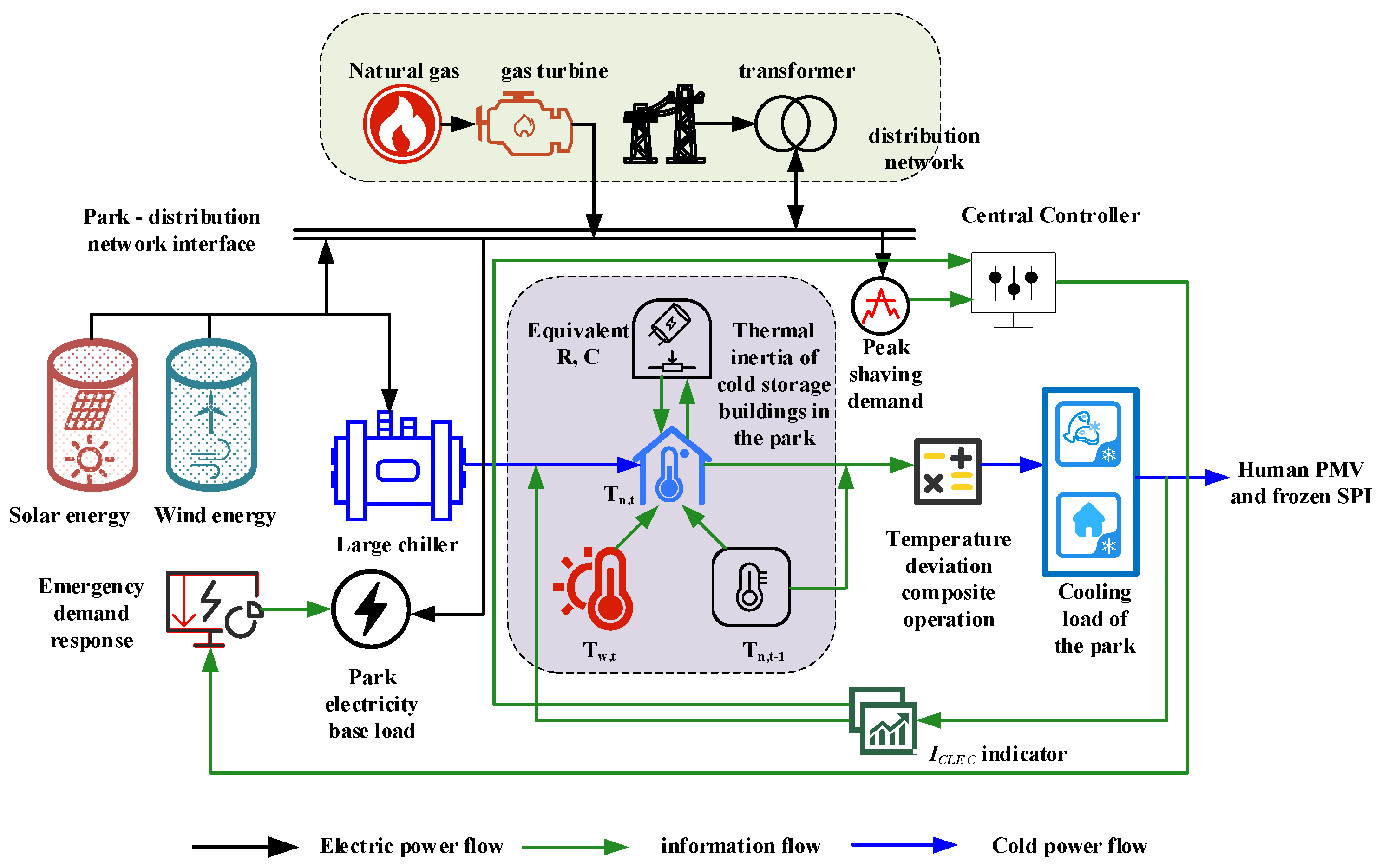
2.1. Total Framework with Diverse Cooling Loads
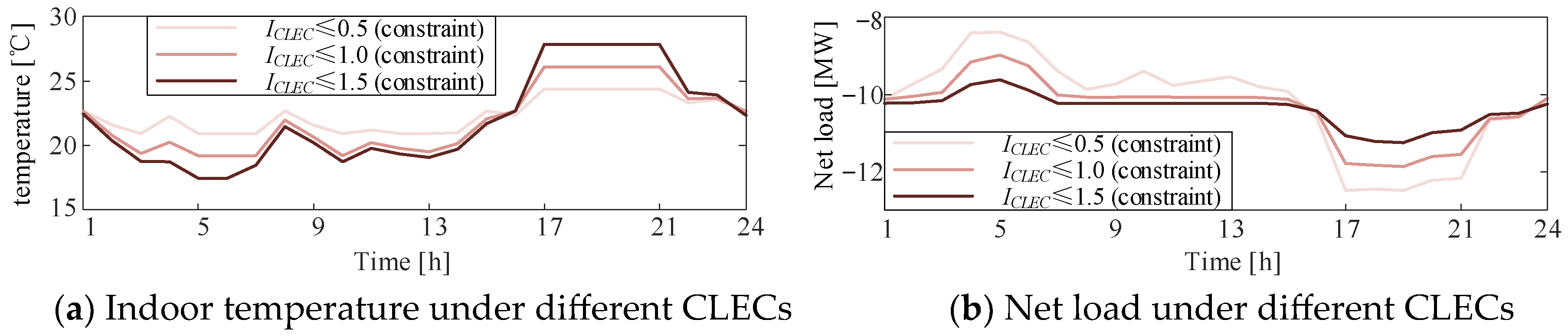
2.2. Modeling of Diverse Cooling Load’s Economic Contribution
3. Methodology
3.1. Day-Ahead Stage
3.1.1. Objective Function
- (1)
- Gas Turbine
- (2)
- Evaluation of peak shaving performance
3.1.2. Constraints
- (1)
- Power-balance constraints
- (2)
- Cooling load constraints
- (3)
- Chiller output constraints
- (4)
- Constraints on power flow
- (5)
- Constraints of renewable energy outputs
3.2. Uncertainty Set
3.3. Intra-Day Stage
3.3.1. Objectives
3.3.2. Remaining Constraints in the Intra-Day Stage
- (1)
- Power balance
- (2)
- Feeder power flow constraints
- (3)
- Emergency demand response constraint
- (4)
- Constraints of renewable energy outputs
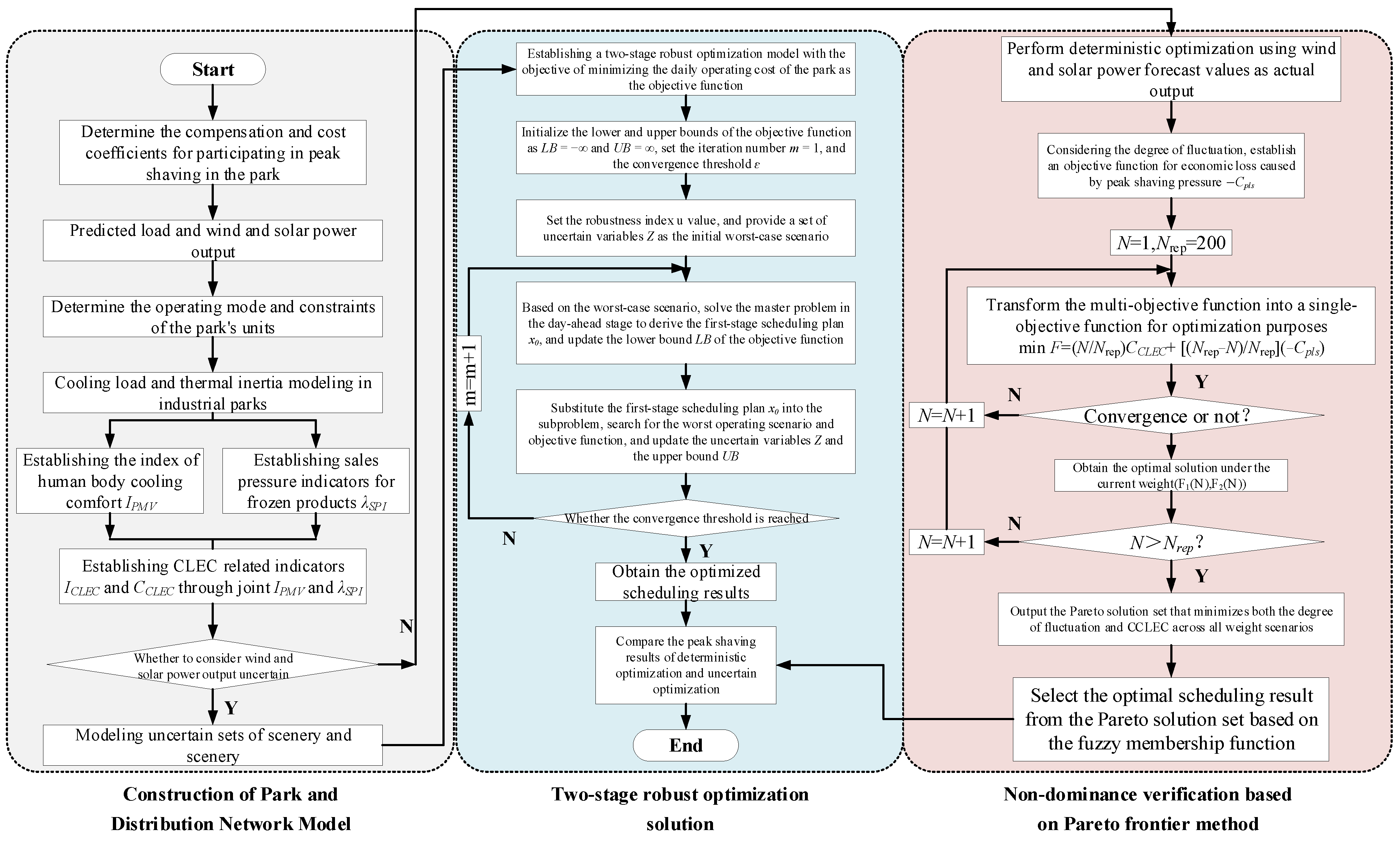
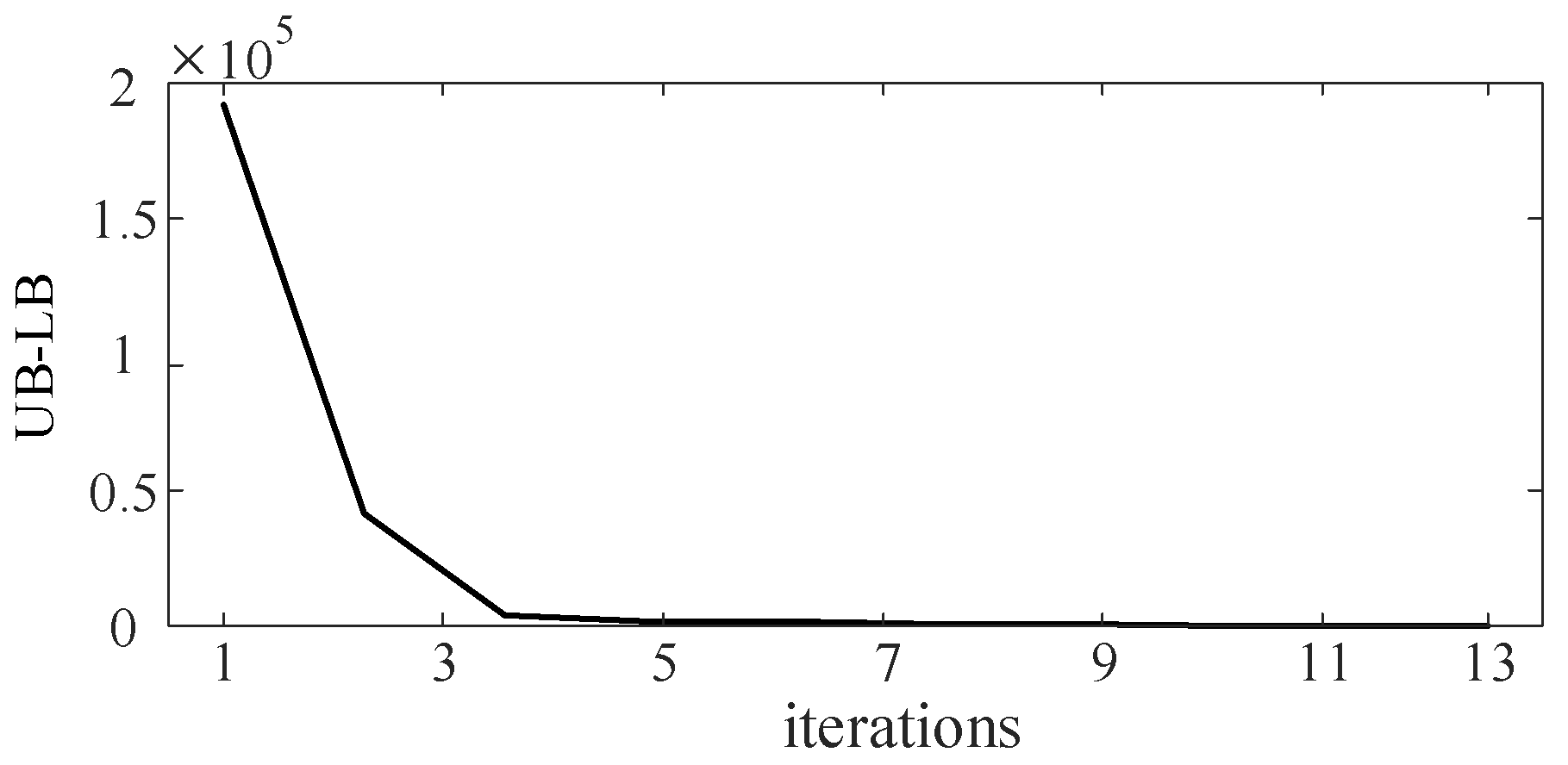
4. Model Solution
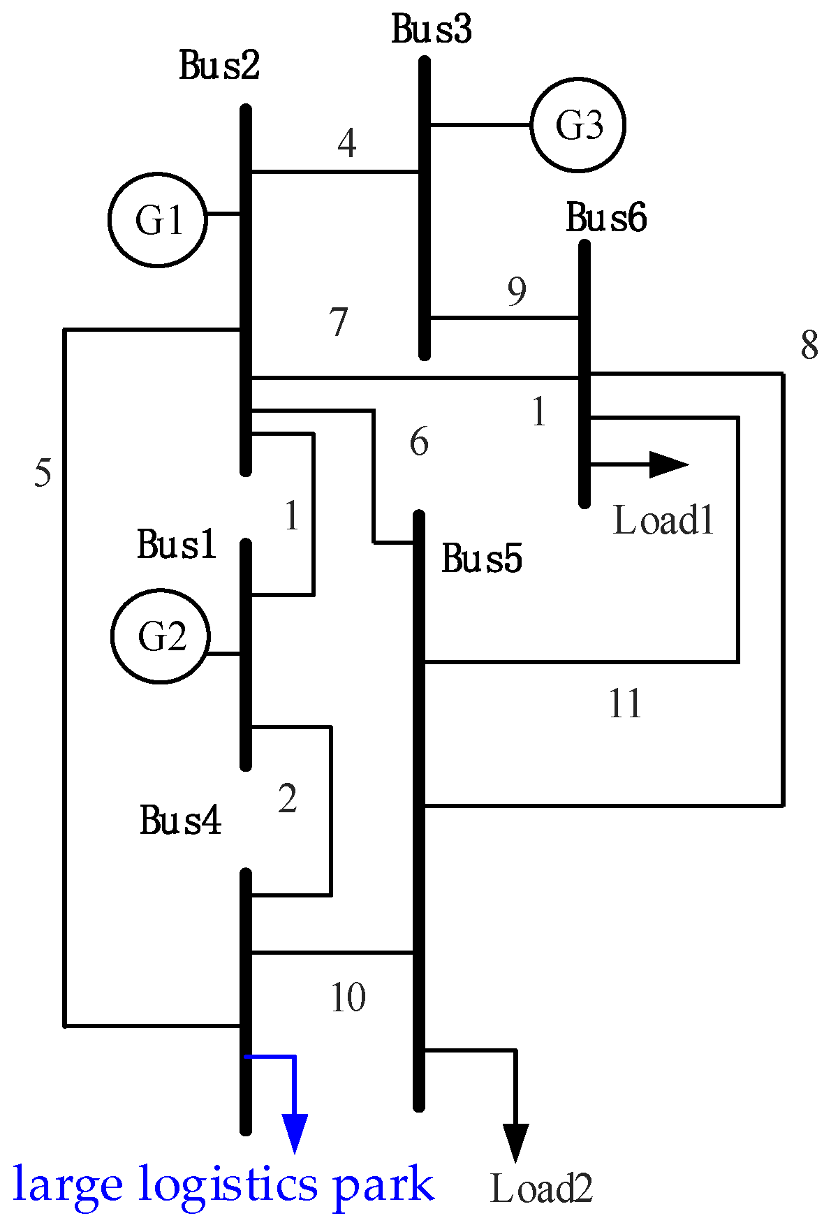
5. Case Studies
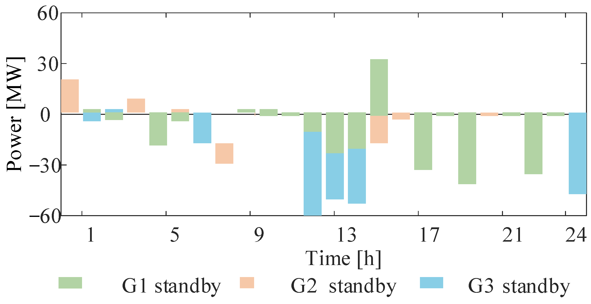
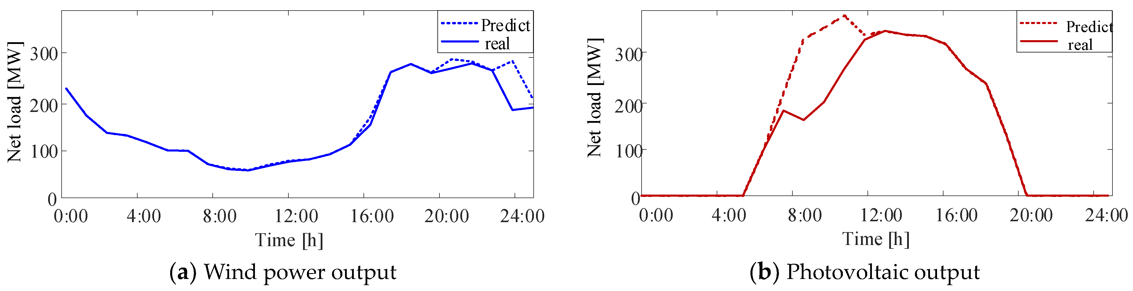
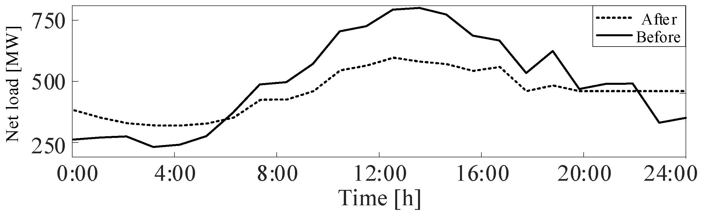
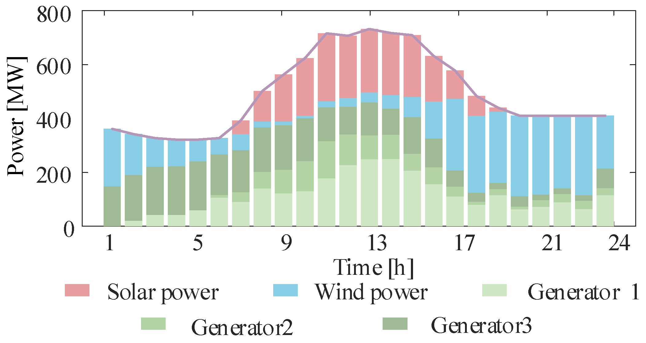
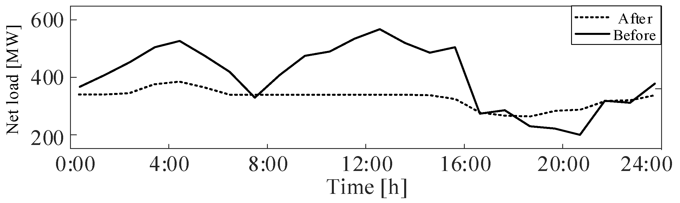
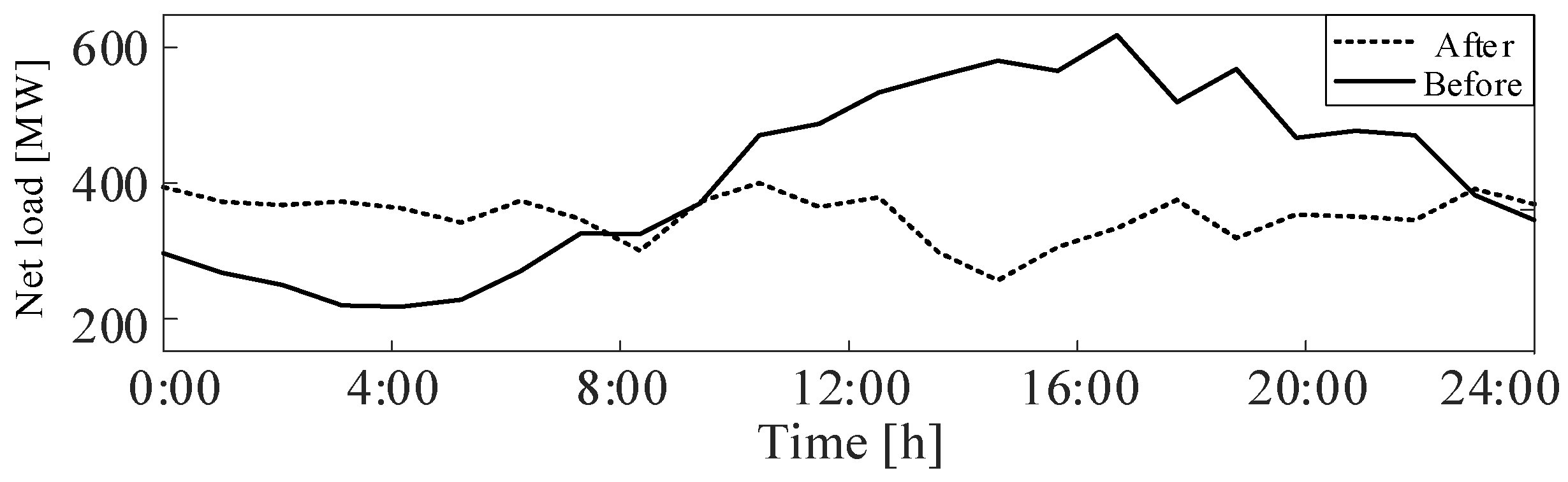
5.1. Peak Shaving, Considering the Uncertainties
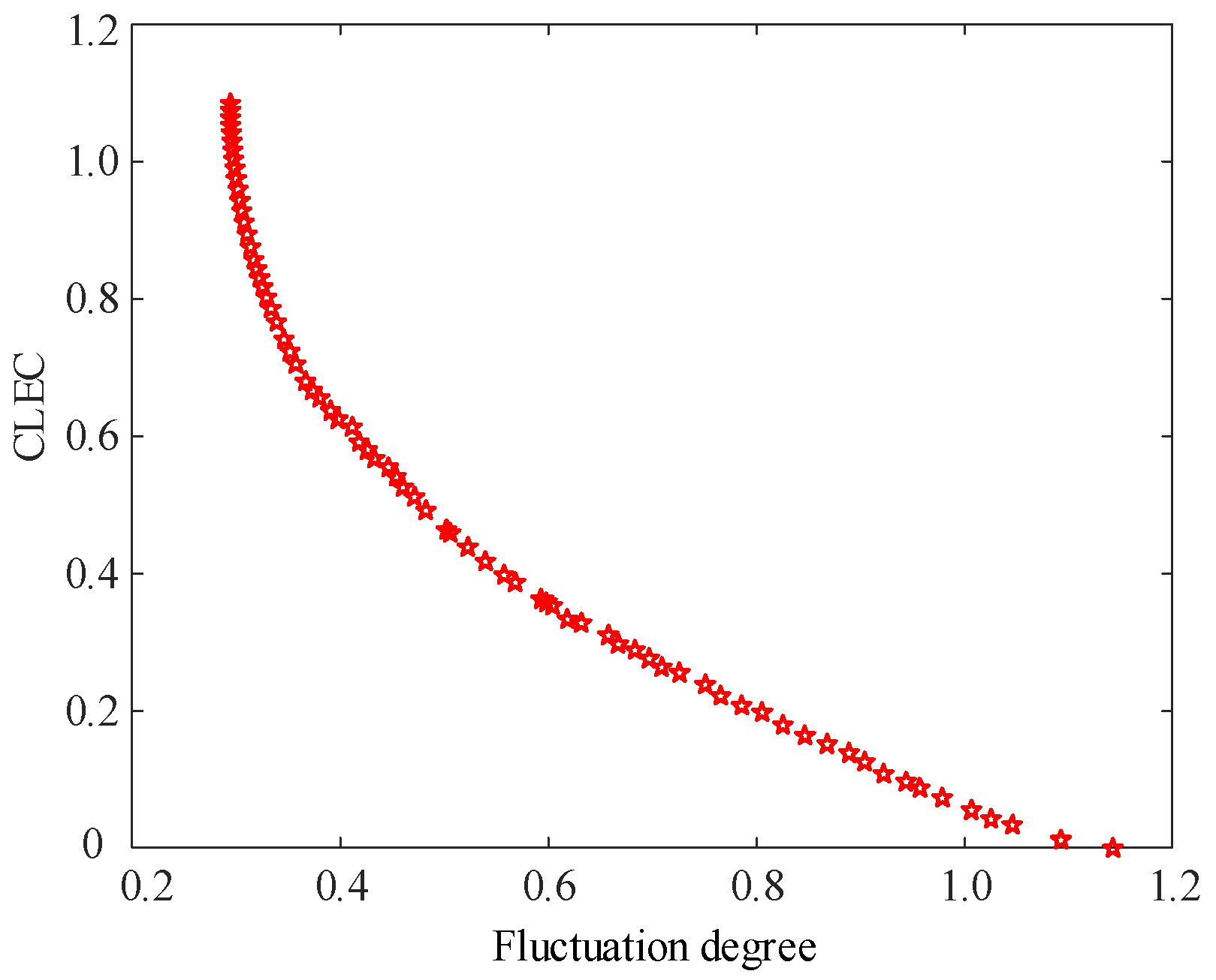
5.2. Non-Domination Verification and Comparative Validation of Indicators
5.3. Comparison Study: Steam Turbine Replacement for Gas Turbine
6. Conclusions
Author Contributions
Funding
Data Availability Statement
Conflicts of Interest
References
- Lin, L.; Xu, B.; Xia, S. Multi-Angle Economic Analysis of Coal-Fired Units with Plasma Ignition and Oil Injection during Deep Peak Shaving in China. Appl. Sci. 2019, 9, 5399. [Google Scholar] [CrossRef]
- Wang, X.; Wu, Y.; Fu, L. Evaluation of combined heat and power plants with electricity regulation. Appl. Therm. Eng. 2023, 227, 120364. [Google Scholar] [CrossRef]
- Liu, Q.; Zhao, J.; Shao, Y.; Wen, L.; Wu, J.; Liu, D.; Ma, Y. Multi-Power Joint Peak-Shaving Optimization for Power System Considering Coordinated Dispatching of Nuclear Power and Wind Power. Sustainability 2019, 11, 4801. [Google Scholar] [CrossRef]
- Yu, Y.; Zhou, G.; Wu, K.; Chen, C.; Bian, Q. Optimal Configuration of Power-to-Heat Equipment Considering Peak-Shaving Ancillary Service Market. Energies 2023, 16, 6860. [Google Scholar] [CrossRef]
- Liao, S.; Zhang, Y.; Liu, J.; Liu, B.; Liu, Z. Short-Term Peak-Shaving Operation of Single-Reservoir and Multicascade Hydropower Plants Serving Multiple Power Grids. Water Resour. Manag. 2021, 35, 689–705. [Google Scholar] [CrossRef]
- Zou, Y.; Hu, Z.; Zhou, S.; Luo, Y.; Han, X.; Xiong, Y.; Li, M.E. Day-Ahead and Intraday Two-Stage Optimal Dispatch Considering Joint Peak Shaving of Carbon Capture Power Plants and Virtual Energy Storage. Sustainability 2024, 16, 2890. [Google Scholar] [CrossRef]
- Zhang, Z.; Cong, W.; Liu, S.; Li, C.; Qi, S. Auxiliary Service Market Model Considering the Participation of Pumped-Storage Power Stations in Peak Shaving. Front. Energy Res. 2022, 10, 915125. [Google Scholar] [CrossRef]
- Liu, B.; Lund, J.R.; Liao, S.; Jin, X.; Liu, L.; Cheng, C. Optimal power peak shaving using hydropower to complement wind and solar power uncertainty. Energy Convers. Manag. 2020, 209, 2621–2631. [Google Scholar] [CrossRef]
- Cheng, X.; Feng, S.; Huang, Y.; Wang, J. A New Peak-Shaving Model Based on Mixed Integer Linear Programming with Variable Peak-Shaving Order. Energies 2021, 14, 887. [Google Scholar] [CrossRef]
- Fang, Y.; Zhao, S.; Chen, Z. Multi-objective unit commitment of jointly concentrating solar power plant and wind farm for providing peak-shaving considering operational risk. Int. J. Electr. Power Energy Syst. 2022, 137, 107754. [Google Scholar] [CrossRef]
- Uddin, M.; Romlie, M.F.; Abdullah, M.F.; Halim, S.A.; Bakar, A.H.A.; Kwang, T.C. A review on peak load shaving strategies. Renew. Sustain. Energy Rev. 2018, 82, 3323–3332. [Google Scholar] [CrossRef]
- Yang, Y.; Wang, Y.; Gao, Y.; Gao, C. Peak Shaving Analysis of Power Demand Response with Dual Uncertainty of Unit and Demand-Side Resources under Carbon Neutral Target. Energies 2022, 15, 4588. [Google Scholar] [CrossRef]
- Shen, J.; Jiang, C.; Liu, Y.; Qian, J. A Microgrid Energy Management System with Demand Response for Providing Grid Peak Shaving. Electr. Mach. Power Syst. 2014, 44, 843–852. [Google Scholar] [CrossRef]
- Su, H.; Feng, D.; Zhao, Y.; Zhou, Y.; Zhou, Q.; Fang, C.; Rahman, U. Optimization of Customer-Side Battery Storage for Multiple Service Provision: Arbitrage, Peak Shaving, and Regulation. IEEE Trans. Ind. Appl. 2022, 58, 2559–2573. [Google Scholar] [CrossRef]
- Alessia, A.; Fabio, P. Assessing the Demand Side Management Potential and the Energy Flexibility of Heat Pumps in Buildings. Energies 2018, 11, 1846. [Google Scholar] [CrossRef]
- Abbasi, A.; Sultan, K.; Afsar, S.; Aziz, M.A.; Khalid, H.A. Optimal Demand Response Using Battery Storage Systems and Electric Vehicles in Community Home Energy Management System-Based Microgrids. Energies 2023, 16, 5024. [Google Scholar] [CrossRef]
- Guelpa, E.; Marincioni, L. Demand side management in district heating systems by innovative control. Energy 2019, 188, 116037. [Google Scholar] [CrossRef]
- Lu, N.; Chassin, D.P.; Widergren, S.E. Modeling uncertainties in aggregated thermostatically controlled loads using a State queueing model. IEEE Trans. Power Syst. 2005, 20, 725–733. [Google Scholar] [CrossRef]
- Bashash, S.; Fathy, H.K. Modeling and control insights into demand-side energy management through setpoint control of thermostatic loads. In Proceedings of the American Control Conference (ACC), San Francisco, CA, USA, 29 June–1 July 2011; pp. 4546–4553. [Google Scholar]
- Khan, S.; Shahzad, M.; Habib, U.; Gawlik, W.; Palensky, P. Stochastic Battery Model for Aggregation of Thermostatically Controlled Loads. In Proceedings of the 2016 IEEE International Conference on Industrial Technology (ICIT), Taipei, Taiwan, 14–17 March 2016; pp. 570–575. [Google Scholar]
- Callaway, D.S. Tapping the energy storage potential in electric loads to deliver load following and regulation, with application to wind energy. Energy Convers. Manag. 2009, 50, 1389–1400. [Google Scholar] [CrossRef]
- Parkinson, S.; Wang, D.; Crawford, C.; Djilali, N. Comfort-Constrained Distributed Heat Pump Management. In Proceedings of the International Conference on Smart Grid and Clean Energy Technologies, Chengdu, China, 27–30 September 2011; Elsevier Ltd.: Chengdu, China, 2011; pp. 849–855. [Google Scholar]
- Ma, Y.; Xu, W.; Yang, H.; Zhang, D. Two-stage stochastic robust optimization model of microgrid day-ahead dispatching considering controllable air conditioning load. Int. J. Electr. Power Energy Syst. 2022, 141, 108174. [Google Scholar] [CrossRef]
- Mendieta, W.; Cañizares, C.A. Primary Frequency Control in Isolated Microgrids Using Thermostatically Controllable Loads. IEEE Trans. Smart Grid 2021, 12, 93–105. [Google Scholar] [CrossRef]
- Li, Z.; Sun, Z.; Meng, Q.; Wang, Y.; Li, Y. Reinforcement learning of room temperature set-point of thermal storage air-conditioning system with demand response. Energy Build. 2022, 259, 111903. [Google Scholar] [CrossRef]
- Nian, F.; Wang, K. Study on indoor environmental comfort based on improved PMV index. In Proceedings of the International Conference on Computational Intelligence & Communication Technology, Ghaziabad, India, 9–10 February 2017; pp. 1–4. [Google Scholar]
- Gormley, R.; Walshe, T.; Hussey, K.; Butler, F. The Effect of Fluctuating vs. Constant Frozen Storage Temperature Regimes on Some Quality Parameters of Selected Food Products. LWT—Food Sci. Technol. 2002, 35, 190–200. [Google Scholar] [CrossRef]
- Yunyang, Z.; Li, Y.; Jiayong, L.I.; Lei, X.; Hao, Y.E.; Zhenzhi, L. Robust Optimal Dispatch of Micro-energy Grid with Multi-energy Complementation of Cooling Heating Power and Natural Gas. Autom. Electr. Power Syst. 2019, 14, 65–72. [Google Scholar]
- Wang, H.; Xing, H.; Luo, Y.; Zhang, W. Optimal scheduling of micro-energy grid with integrated demand response based on chance-constrained programming. Int. J. Electr. Power Energy Syst. 2023, 144, 1086. [Google Scholar] [CrossRef]
- Zhang, Z.; Zhou, M.; Chen, Y.; Li, G. Exploiting the operational flexibility of AA-CAES in energy and reserve optimization scheduling by a linear reserve model. Energy 2023, 263, 126084. [Google Scholar] [CrossRef]
- Amin, G.R. A comment on modified big-M method to recognize the infeasibility of linear programming models. Knowl. -Based Syst. 2010, 23, 283–284. [Google Scholar] [CrossRef]
- Meshram, M.S.; Sahu; Omprakash; Preeti, R. Application of ANN in Economic Generation Scheduling in IEEE 6-Bus System. Int. J. Eng. Sci. Technol. 2011, 3, 2461–2466. [Google Scholar]
- Li, H.; Zhao, T.; Dian, S. Forward search optimization and subgoal-based hybrid path planning to shorten and smooth global path for mobile robots. Knowl.-Based Syst. 2022, 258, 110034. [Google Scholar] [CrossRef]
- Zhang, Z.; Wang, K.; Zhu, L.; Wang, Y. A Pareto improved artificial fish swarm algorithm for solving a multi-objective fuzzy disassembly line balancing problem. Expert Syst. Appl. 2017, 86, 165–176. [Google Scholar] [CrossRef]
- Antonsson, E.K.; Sebastian, H. Fuzzy fitness functions applied to engineering design problems. Eur. J. Oper. Res. 2005, 166, 794–811. [Google Scholar] [CrossRef]
- Jamali, A.; Mallipeddi, R.; Salehpour, M.; Bagheri, A. Multi-objective differential evolution algorithm with fuzzy inference-based adaptive mutation factor for Pareto optimum design of suspension system. Swarm Evol. Comput. 2020, 54, 100666. [Google Scholar] [CrossRef]


| PMV | −3 | −2 | −1 | 0 | 1 | 2 | 3 |
|---|---|---|---|---|---|---|---|
| Sensation | Cold | Cool | Slightly cool | Neutral | Slightly warm | Warm | Hot |
| Bus-i | Pd | Qd | baseKV | Vmax | Vmin |
|---|---|---|---|---|---|
| 1 | 0 | 0 | 230 | 1.05 | 1.05 |
| 2 | 0 | 0 | 230 | 1.05 | 1.05 |
| 3 | 0 | 0 | 230 | 1.07 | 1.05 |
| 4 | 70 | 80 | 230 | 1.05 | 0.95 |
| 5 | 80 | 74 | 230 | 1.05 | 0.95 |
| 6 | 90 | 79 | 230 | 1.05 | 0.95 |
| Case | Total Cost [USD] | Backup Volume Used [MW] | CCLEC | Cfls | EDR [MW] |
|---|---|---|---|---|---|
| 1 | 17,154.3 | 417 | 1725.1 | 5351.6 | 168.5 |
| 2 | 17,889.5 | 464 | 1811.6 | 4945.8 | 136.9 |
| 3 | 18,501.8 | 637 | 1904.9 | 4410.7 | 52.6 |
| 4 | 19,021.1 | 669 | 1991.2 | 4291.4 | 10 |
| Indicator | Before | After | Performance [%] |
|---|---|---|---|
| PVD | 547.09 | 296.43 | 45.82 |
| FV | 2890.7 | 1312.9 | 54.59 |
| PMV | 0.9445 | 0.5750 | 39.12 |
| SPI | 0.9347 | 0.6883 | 26.36 |
| Case | Total Cost [USD] | Reserve Capacity Used [MW] | CCLEC | Cfls | EDR [MW] |
|---|---|---|---|---|---|
| The deterministic optimization method | 15,842.6 | 0 | 1516.8 | 5560.1 | 512.9 |
| Case 4 | 19,021.1 | 669 | 1991.2 | 4291.4 | 10 |
| Case | Total Cost [USD] | CCLEC | Cfls | EDR [MW] | PVD Enhancement [%] | FV Enhancement [%] |
|---|---|---|---|---|---|---|
| Gas turbine | 19,021.1 | 1991.2 | 4291.4 | 10 | 45.82 | 54.59 |
| Steam turbine | 15,617.5 | 2076.9 | 3945.8 | 191.9 | 31.08 | 42.27 |
Disclaimer/Publisher’s Note: The statements, opinions and data contained in all publications are solely those of the individual author(s) and contributor(s) and not of MDPI and/or the editor(s). MDPI and/or the editor(s) disclaim responsibility for any injury to people or property resulting from any ideas, methods, instructions or products referred to in the content. |
© 2024 by the authors. Licensee MDPI, Basel, Switzerland. This article is an open access article distributed under the terms and conditions of the Creative Commons Attribution (CC BY) license (https://creativecommons.org/licenses/by/4.0/).
Share and Cite
Zhou, J.; Zhang, J.; Qiu, Z.; Yu, Z.; Cui, Q.; Tong, X. Two-Stage Robust Optimization for Large Logistics Parks to Participate in Grid Peak Shaving. Symmetry 2024, 16, 949. https://doi.org/10.3390/sym16080949
Zhou J, Zhang J, Qiu Z, Yu Z, Cui Q, Tong X. Two-Stage Robust Optimization for Large Logistics Parks to Participate in Grid Peak Shaving. Symmetry. 2024; 16(8):949. https://doi.org/10.3390/sym16080949
Chicago/Turabian StyleZhou, Jiu, Jieni Zhang, Zhaoming Qiu, Zhiwen Yu, Qiong Cui, and Xiangrui Tong. 2024. "Two-Stage Robust Optimization for Large Logistics Parks to Participate in Grid Peak Shaving" Symmetry 16, no. 8: 949. https://doi.org/10.3390/sym16080949