Abstract
The Hosoya index is an important topological index in graph theory, which is defined as the total number of s-matchings, denoted as , in a graph G. Therefore, computing the number of s-matchings for various molecular structures holds significant importance. By applying the concept of symmetry, defining the s-matching vector of the graph with a specified edge, using the transfer matrix, and iteratively applying two recursive formulas to derive the reduction formula, we compute the number of s-matchings of cyclooctatetraene chains.
1. Introduction
Over the past few years, chemists have shown great interest in cyclooctatetraene and its derivatives, leading to their wide-ranging applications in various industries. Its discovery can be attributed to a chemical experiment conducted by the German chemist Willstätter and his colleagues through chemical synthesis. Since its discovery, cyclooctatetraene has proven to be an invaluable intermediate in organic synthesis and a versatile stereo ligand in organometallic chemistry. Also known as “1, 3, 5, 7-cyclooctatetraene”, this organic compound falls under the category of olefins, with the chemical formula . It is a colorless to pale yellow liquid, soluble in ethanol, slightly soluble in acetone and benzene, but insoluble in water. Despite sharing some characteristics of rotational alkenes and unsaturated hydrocarbons with benzene, cyclooctatetraene is neither aromatic nor antiaromatic, making it incompatible with Hückel’s rule analysis. Cyclooctatetraene is primarily used as a solvent and laboratory reagent, and finds widespread applications in the synthesis of fibers, dyes, pharmaceutical products, and other industrial products. However, due to the cessation of industrial production, cyclooctatetraene has become one of the more costly materials in the market in recent years. The significance of cyclooctatetraene chains in chemistry lies in their ability to allow chemists to study and enhance the stability and reactivity of antiaromatic molecules. By forming chain structures or functionalizing them, it is possible to modulate the molecule’s electronic structure and chemical behavior, which is crucial for organic synthesis, materials science, and theoretical chemistry. Research on cyclooctatetraene chains not only expands the possibilities of molecular design but also provides a theoretical and experimental foundation for developing new functional materials. To delve deeper into the properties and characteristics of cyclooctatetraene, we can refer to the comprehensive studies conducted by researchers in [1,2,3,4,5]. In particular, the authors [5] focused on analyzing the expected values of the Kirchhoff index for random cyclooctatetraene chain. In this paper, we will specifically investigate cyclooctatetraene chains in which each octagon is adjacent to a maximum of two octagons, as depicted in Figure 1.
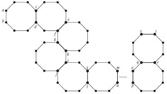
Figure 1.
A cyclooctatetraene chain.
Let G be a simple graph. and are the set of vertices and the set of edges of the graph G, respectively. For any two edges in a graph G, they are said to be independent edges of the graph G if neither of them is adjacent in the graph G, that is, they do not share a common vertex. The set of independent edges in a graph G is called a matching. A s-matching is a matching that contains s-independent edges, and the maximum possible value of s-matching in a graph G is called the number of s-matchings and is denoted by . In 1971, Haruo Hosoya defined a topological index, the Hosoya index [6], as
Note that s takes values from 0 here.
The introduction of the Hosoya index triggered the proposal of a large number of topological indices, such as the Merrifield–Simmons index. For a study of the combination of these two indices for graphs, see [7,8,9,10,11]. Among the numerous topological indices, the Hosoya index has explicit and specific properties and is therefore often used to study a number of different issues concerning organic molecules in chemical graph theory; see [12,13,14,15,16] for more details.
The computation of the number of s-matchings of organic compounds or graphs with given constraints has been a hot topic in chemical graph theory. When , in-depth findings regarding the computation of s-matchings for a specific graph are detailed in references [17,18,19]. Additional research literature on computing the number of s-matchings for special graphs is available in [20,21,22,23].
In chemical graph theory, combinatorial enumeration problems, such as computing the number of matches of a graph, can be solved through the iterative application of established recurrence relationships. However, when dealing with large and relatively complex systems, it is often difficult to obtain the desired results with these methods, even when using computers. Hosoya and Ohkami [24], and Randić et al. [25] proposed two highly effective and pragmatic methods to overcome these difficulties, known as the operator and transfer matrix techniques. The transfer matrix method, which we can find in [26,27,28,29], is easier to use. The transfer matrix method is a well-established method for analyzing the structure of organic molecules with a chain character. In [24], Hosoya and Ohkami used the operator technique to obtain the characterization, matching, and related recursive equations of line shapes. In addition, in some periodic lattice spaces, Hosoya and Motoyama also utilized operator techniques with details given in [30].
In this paper, we explore the Hosoya index. The Hosoya index is widely used in structure-property modeling and is a significant topic in mathematical chemistry research, with further details available in [31,32]. In [33], Mert Sinan Oz introduced the concept of a s-matching vector and employed the transfer matrix technique to compute the number of s-matchings in benzenoid chains. Based on these studies, here, it is quite natural and interesting for us to consider the Hosoya index for random cyclooctatetraene chains. In this paper, by applying the concept of symmetry, we first define a s-matching vector for a given edge in the graph G, using the s-matching vector and two recursive formulas. Then, we compute the four numbers of s-matchings one by one, by iteratively removing one edge at a time. Through iterative derivation with the recursive formulas, we derive five reduction formulas and construct five dimensional transfer matrices. Ultimately, we can use the reduction formulas and transfer matrices to qualitatively compute the number of s-matchings for any cyclooctatetraene chain with the help of the introduced algorithm. This paper integrates operator techniques with transfer matrix techniques, facilitating easier computation in MATLAB. Therefore, the method mentioned earlier can be used to compute the Hosoya index of more complex random polygonal chains containing n regular polygons. However, it is limited to cases where the number of edges is even.
2. Computation of s-Matchings in Cyclooctatetraene Chains
The recursive formula that is the most essential for computing the s-matching number of a graph G is provided below:
where and are two connected parts of G.
for an edge , see [24] for more information. In the following definition, we will provide a s-matching vector for a given edge in graph G in order to calculate of G.
Definition 1
([33]). Let us consider a graph G and as an edge in G. The s-matching vector of G on edge is defined as given below:
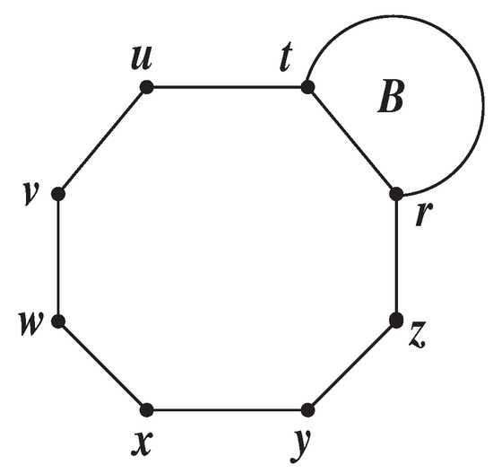
Theorem 1.
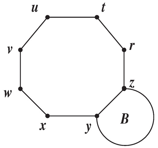
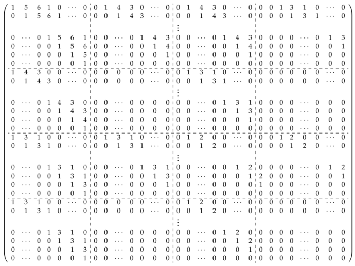
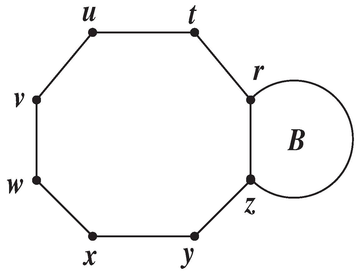
Let be a graph formed by combining the edges of the graph B with a cyclooctatetraene on the edge of the graph B (See Figure 2). Then,
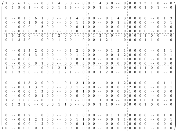
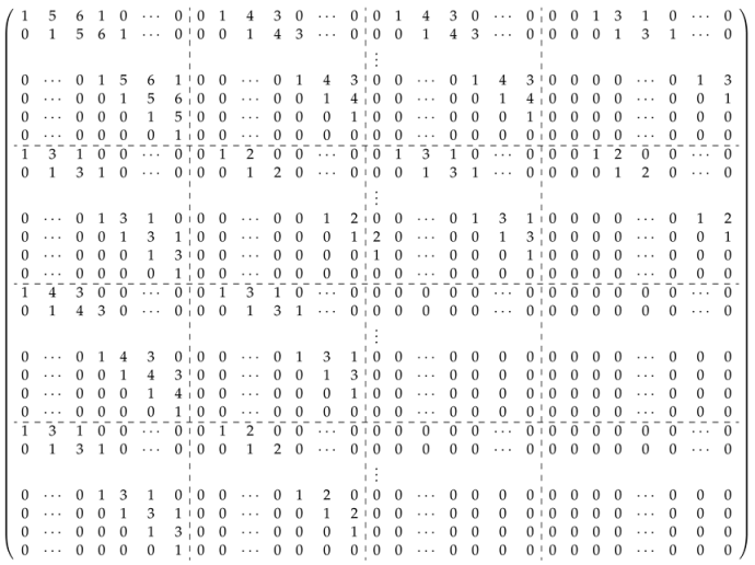
where T is a dimensional transfer matrix as follows:
Figure 2.
Graph in Theorem 1.
Proof.
We shall compute , , and by removing the edges and ; then, by using the recurrence relations 1 and 2 we obtain:
According to the definition of an s-matching vector of G at the edge , the vectors
and
are the first, -th, -th and -th rows of the coefficient matrix, respectively. In addition, it is necessary to calculate , ⋯, , , , ⋯, , , , ⋯, , and , ⋯, , to obtain . It is not really necessary to calculate these values separately, as they can be obtained from the product of a vector and from the above equations. Thus, after calculating the first, -th, -th and -th rows, we obtain the trapezoidal coefficient matrix consisting of sixteen submatrices. As a result, we obtain , where T is a dimensional transfer matrix. □
Clearly, if B is isomorephic to where is path graph with two vertices, then
Theorem 2.

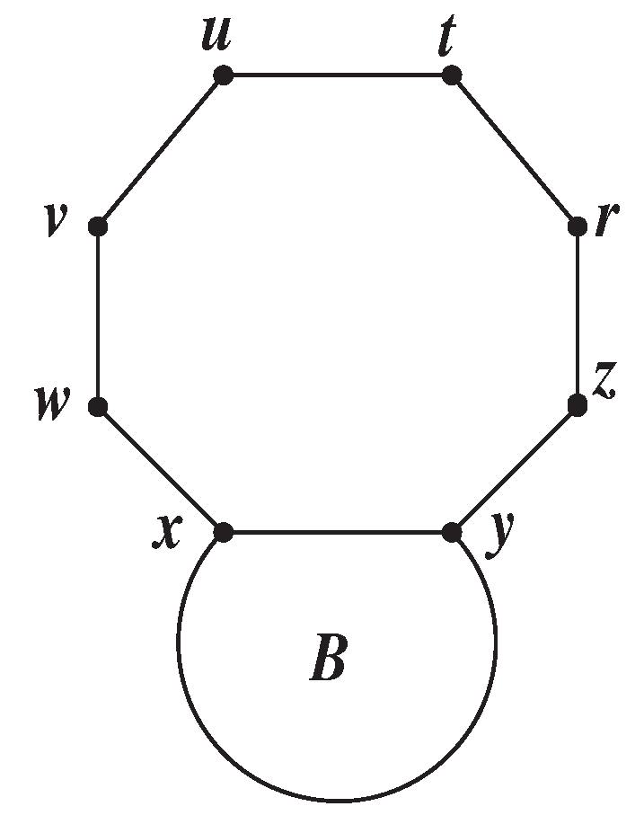
Let be a graph formed by combining the edges of the graph B with a cyclooctatetraene on the edge of the graph B (See Figure 3). Then,
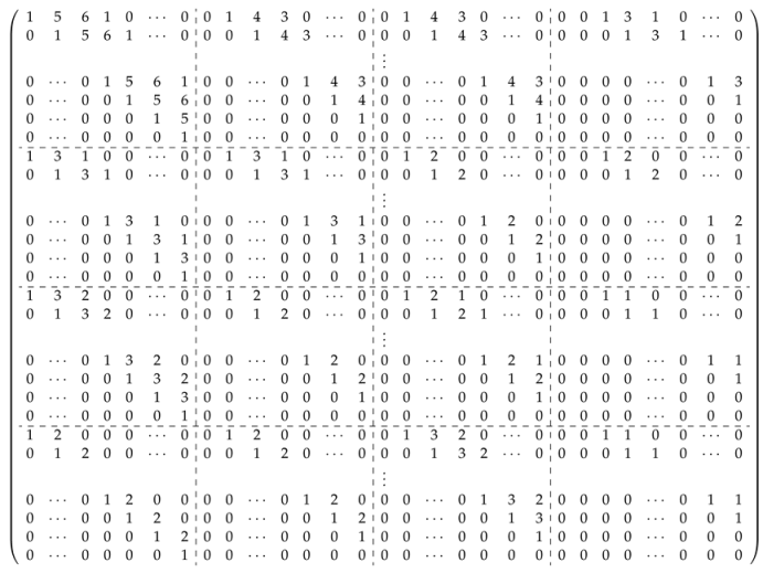
where W is a dimensional transfer matrix as follows:
Figure 3.
Graph in Theorem 2.
Proof.
It is necessary to calculate the values , , and by deleting the particular edges and to obtain the subgraph B that does not include the octagon. Afterwards, we will utilize the recurrence relations 1 and 2 as follows:
According to the definition of an s-matching vector of G at the edge , the vectors
and
are the first, -th, -th and -th rows of the coefficient matrix, respectively. We also need to calculate , ⋯, , , , ⋯, , , , ⋯, , and , ⋯, , to obtain . Then, we derive these values as a product of the vector and . After that, we obtain the coefficient matrix consisting of the sixteen partial submatrices in echelon form. Consequently, we obtain the equation , where W is a dimensional transfer matrix. □
Theorem 3.
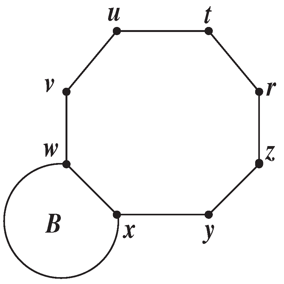
Let be a graph formed by combining the edges of the graph B with a cyclooctatetraene on the edge of the graph B (See Figure 4). Then,
where X is a dimensional transfer matrix as follows:
Figure 4.
Graph in Theorem 3.
Proof.
As shown in the previous proof, first, we need to calculate the values , , and by deleting the edges and . Next, we use the recurrence relations 1 and 2 as shown below:
According to the definition of a s-matching vector of G at the edge , the vectors
and
are the first, -th, -th and -th rows of the coefficient matrix, respectively. At the same time, the values , ⋯, , , , ⋯, , , , ⋯, , and , ⋯, , need to be calculated to obtain . Then, we shall derive these values as a product of the vector and using the above equations. Next, we will obtain the coefficient matrix consisting of the sixteen partial submatrices in echelon form. Therefore, we obtain , where X is a dimensional transfer matrix. □
Theorem 4.
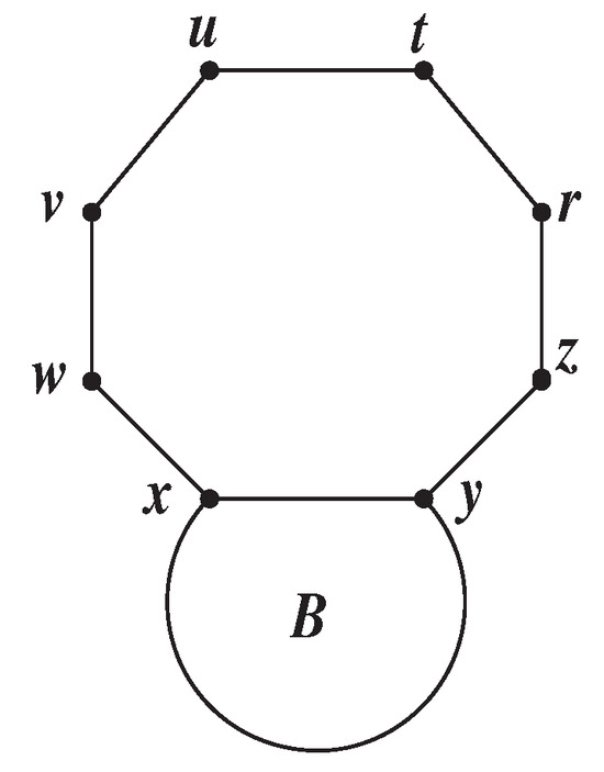
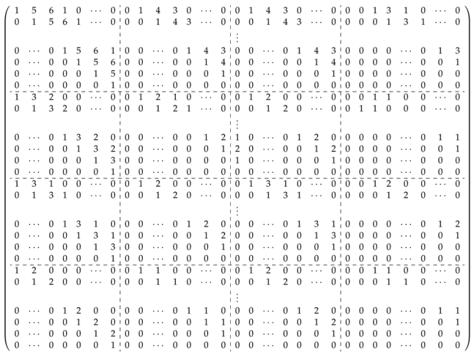
Let be a graph formed by combining the edges of the graph B with a cyclooctatetraene on the edge of the graph B (See Figure 5). Then,
where Y is a dimensional transfer matrix as follows:
Figure 5.
Graph in Theorem 4.
Proof.
To start with, it is necessary to calculate the values , , and by deleting the edges and . After calculating these values, we apply recurrence relations 1 and 2 in the following manner:
According to the definition of an s-matching vector of G at the edge , the vectors
and
are the first, -th, -th and -th rows of the coefficient matrix, respectively. We also need to calculate , ⋯, , , , ⋯, , , , ⋯, , and , ⋯, , to obtain . Nonetheless, we do not need to calculate these values again, because we can derive them as the product of the vector and using the equations we proved above. Then, we can obtain a matrix of trapezoidal coefficients for each of the sixteen parts. Thus, we obtain where Y is a dimensional transfer matrix. □
Theorem 5.

Let be a graph formed by combining the edges of the graph B with a cyclooctatetraene on the edge of the graph B (See Figure 6). Then,
where Z is a dimensional transfer matrix as follows:
Figure 6.
Graph in Theorem 5.
Proof.
To compute the values of , , and , we remove the edges and , similar to what we performed previously.
According to the definition of an s-matching vector of G at the edge , the vectors
and
are the first, -th, -th and -th rows of the coefficient matrix, respectively. After calculating the above values, we still need to calculate , ⋯, , , , ⋯, , , , ⋯, , and , ⋯, , to obtain . Next, we derive these values as the product of the vector and using the equations we proved above. Then, we show that the coefficient matrix is in echelon form in each of the sixteen parts. Consequently, we obtain the equation , where Z is a dimensional transfer matrix. □
3. Algorithms
In this section, we show two algorithms developed in MATLAB that provide a more direct approach to determine the forms of transfer matrices T, W, X, Y, Z and , which were introduced in Section 2. Algorithm 1 calculates the sixteen components of the matrices in echelon form, as described in the proofs of Theorems 1–5. It utilizes the user input value of s to generate these components. Algorithm 2 focuses on obtaining the s-matching vector of at edge when given the values of s and the edge in the path graph . The obtained vector is as follows:
Using Algorithm 1, we determine the transfer matrices T, W, X, Y, Z based on the given value of s. Additionally, we incorporate a few additional steps prior to the step in order to arrange these matrices. Let us outline these steps.
To construct the transfer matrix T, we integrate the following steps sequentially.
; ; ; ; ; ; ; ; ; ; ; ; ; ; ; ; ; ; ; ; ; ; ; ; ; ; ; ; ; ; ; ; ; ; ; ; ; ; ; ; ; ; ; ; .
To construct the transfer matrix W, we integrate the following steps sequentially.
; ; ; ; ; ; ; ; ; ; ; ; ; ; ; ; ; ; ; ; ; ; ; ; ; ; ; ; ; ; ; ; ; ; ; ; ; ; ; ; ; ; ; ; ; .
To construct the transfer matrix X, we integrate the following steps sequentially.
; ; ; ; ; ; ; ; ; ; ; ; ; ; ; ; ; ; ; ; ; ; ; ; ; ; ; ; ; ; ; ; ; ; ; ; ; .
To construct the transfer matrix Y, we integrate the following steps sequentially.
; ; ; ; ; ; ; ; ; ; ; ; ; ; ; ; ; ; ; ; ; ; ; ; ; ; ; ; ; ; ; ; ; ; ; ; ; ; ; ; ; ; ; ; .
To construct the transfer matrix Z, we integrate the following steps sequentially.
; ; ; ; ; ; ; ; ; ; ; ; ; ; ; ; ; ; ; ; ; ; ; ; ; ; ; ; ; ; ; ; ; ; ; ; ; .
| Algorithm 1: Algorithm for setting up the transfer matrix forms T, W, X, Y, Z for the corresponding s. |
Input: Enter the value of s. Result: Required echelon matrix form depending on the rows 1, , , . ; “Here, the steps given after adding this algorithm will be based on the needed matrix”; ; ; ; ; for do for s do ; ; ; ; end end for do for s do ; ; ; ; end end for do for s do ; ; ; ; end end for do for s do ; ; ; ; end end |
| Algorithm 2: Design the algorithm to calculate in which u and v represent vertices of graph . |
Input: Enter the value of s. ; ; ; ; ; ; ; Result: . |
4. Concluding Remarks
In this paper, we prove that any number of s-matchings can be calculated using the defined s-matching vector and the matrices T, W, X, Y, Z for any cyclooctatetraene chain. In particular, by using the s-matching vector, we can obtain not only the s-matching numbers of any cyclooctatetraene chain but also the Hosoya index associated with the respective cyclooctatetraene chain. This implies that in the future, the computation of the Hosoya index for a chain of random polygons containing n regular polygons can be facilitated more conveniently using this methodology.
Author Contributions
Conceptualization, S.C.; methodology, X.G.; software, H.H.; validation, S.C., H.H. and X.G.; formal analysis, H.H.; investigation, S.C.; resources, X.G.; data curation, S.C.; writing—original draft preparation, S.C.; writing—review and editing, S.C.; visualization, S.C.; supervision, S.C.; project administration, X.G.; funding acquisition, X.G. All authors have read and agreed to the published version of the manuscript.
Funding
The research is partially supported by National Science Foundation of China (Grant No. 11671164) and Natural Science Foundation of Anhui Province (Grant No. 2008085MA01) and Humanity and Social Science Research Project of Anhui Educational Committee (Grant No. SK2019A0095).
Data Availability Statement
Data are contained with the article.
Conflicts of Interest
The authors declare no conflicts of interest.
References
- Gottfriedsen, J.; Miloslavina, A.; Edelmann, F.T. Cyclooctatetraene made easy. Tetrahedron Lett. 2004, 45, 3583–3584. [Google Scholar] [CrossRef]
- Chang, J.L.; Cheng, M.Z.; Huang, Y.J. Theoretical Study of the Negative Ion Photoelectron Spectrum of Cyclooctatetraene via Computation of Franck-Condon Factors. J. Phys. Chem. A 2020, 124, 3205–3213. [Google Scholar] [CrossRef]
- Deslongchamps, G.; Deslongchamps, P. Bent Bonds (τ) and the Antiperiplanar Hypothesis-The Chemistry of Cyclooctatetraene and Other C8H8 Isomers. J. Org. Chem. 2018, 83, 5751–5755. [Google Scholar] [CrossRef]
- Tomilin, O.B.; Fomina, L.V.; Rodionova, E.V. Possible Skeletal Transformations of Cyclooctatetraene in Its Thermal Isomerization. Russ. J. Org. Chem. 2022, 58, 488–498. [Google Scholar] [CrossRef]
- Qi, J.F.; Ni, J.B.; Geng, X.Y. The expected values for the Kirchhoff indices in the random cyclooctatetraene and spiro chains. J. Discret. Applited Math. 2022, 321, 240–249. [Google Scholar] [CrossRef]
- Hosoya, H. Topological Index. A Newly Proposed Quantity Characterizing the Topological Nature of Structural Isomers of Saturated Hydrocarbons. Bull. Chem. Soc. Jpn. 1971, 44, 2332–2339. [Google Scholar] [CrossRef]
- Ye, Y.L.; Pan, X.F.; Liu, H.Q. Ordering unicyclic graphs with respect to Hosoya indices and Merrifield-Simmons indices. Match-Commun. Math. Comput. Chem. 2008, 59, 191–202. [Google Scholar]
- Huang, G.H.; Wu, R.F.; Deng, H.Y. The expected values of Hosoya index and Merrifield-Simmons index in a random spiro chain. Util. Math. 2019, 110, 195–202. [Google Scholar]
- Bai, Y.L.; Zhao, B.; Zhao, P.Y. Extremal Merrifield-Simmons Index and Hosoya Index of Polyphenyl Chains. Match-Commun. Math. Comput. Chem. 2009, 62, 649–656. [Google Scholar]
- Huang, G.H.; Kuang, M.J.; Deng, H.Y. The expected values of Hosoya index and Merrifield-Simmons index in a random polyphenylene chain. J. Comb. Optim. 2016, 32, 550–562. [Google Scholar] [CrossRef]
- Yang, W.L. Hosoya and Merrifleld-Simmons Indices in Random Polyphenyl Chains. Acta Math. Appl. Sin. Engl. Ser. 2021, 37, 485–494. [Google Scholar] [CrossRef]
- Hosoya, H. Important mathematical structures of the topological index Z for tree graphs. J. Chem. Inf. Model. 2007, 47, 744–750. [Google Scholar] [CrossRef]
- Ou, J. On acyclic molecular graphs with maximal Hosoya index, energy, and short diameter. J. Math. Chem. 2008, 43, 328–337. [Google Scholar] [CrossRef]
- Ou, J. On extremal unicyclic molecular graphs with maximal Hosoya index. Discrete Appl. Math. 2009, 157, 391–397. [Google Scholar] [CrossRef]
- Li, S.C.; Zhu, Z.X. On the Hosoya index of unicyclic graphs with a given diameter. ARS Comb. 2014, 114, 111–128. [Google Scholar]
- Qiao, Y.F.; Zhan, F.Q. Ordering polygonal chains with respect to Hosoya index. Appl. Math.-J. Chin. Univ. Ser. B 2012, 27, 305–319. [Google Scholar] [CrossRef]
- Behmaram, A. On the Number of 4-Matchings in Graphs. Match-Commun. Math. Comput. Chem. 2009, 62, 381–388. [Google Scholar]
- Vesalian, R.; Asgari, F. Number of 5-Matchings in Graphs. Match-Commun. Math. Comput. Chem. 2013, 69, 33–46. [Google Scholar]
- Vesalian, R.; Namazi, R.; Asgari, F. Number of 6-Matchings in Graphs. Match-Commun. Math. Comput. Chem. 2015, 73, 239–265. [Google Scholar]
- Zeng, Y.Q.; Zhang, F.J. Extremal polyomino chains on k-matchings and k-independent sets. J. Math. Chem. 2007, 42, 125–140. [Google Scholar] [CrossRef]
- Cao, Y.F.; Zhang, F.J. Extremal polygonal chains on k-matchings. Match-Commun. Math. Comput. Chem. 2008, 60, 217–235. [Google Scholar]
- Liu, Y.; Su, X.L.; Xiong, D.N. Integer k-matchings of graphs: k-Berge-Tutte formula, k-factor-critical graphs and k-barriers. Discret Appl. Math. 2021, 297, 120–128. [Google Scholar] [CrossRef]
- Behmaram, A.; Azari, H.Y.; Ashrafi, A.R. On the Number of Matchings and Independent Sets in (3,6)-Fullerenes. Match-Commun. Math. Comput. Chem. 2013, 70, 525–532. [Google Scholar]
- Hosoya, H.; Ohkami, N. Operator technique for obtaining the recursion formulas of characteristic and matching polynomials as applied to polyhex graphs. J. Comput. Chem. 1983, 4, 585–593. [Google Scholar] [CrossRef]
- Randić, M.; Hosoya, H.; Polansky, O.E. On the construction of the matching polynomial for unbranched catacondensed benzenoids. J. Comput. Chem. 1989, 10, 683–697. [Google Scholar]
- Mayer, V. Nonsquare transfer-matrix technique applied to the simulation of electronic diffraction by a three-dimensional circular aperture. Phys. Rev. E 2000, 61, 5953–5960. [Google Scholar] [CrossRef]
- Feyzollahzadeh, M.; Bamdad, M. An efficient technique in transfer matrix method for beam-like structures vibration analysis. Proc. Inst. Mech. Eng. Part C-J. Eng. Mech. Eng. Sci. 2022, 236, 7641–7656. [Google Scholar] [CrossRef]
- Dastjerdi, S.; Abbasi, M. A vibration analysis of a cracked micro-cantilever in an atomic force microscope by using transfer matrix method. Ultramicroscopy 2019, 196, 33–39. [Google Scholar] [CrossRef]
- Krauss, W. Ryan, Computationally efficient modeling of flexible robots using the transfer matrix method. J. Vib. Control. 2012, 18, 596–608. [Google Scholar] [CrossRef]
- Hosoya, H.; Motoyama, A. An effective algorithm for obtaining polynomials for dimer statistics. Application of operator technique on the topological index to two-and three-dimensional rectangular and torus lattices. J. Math. Phys. 1985, 26, 157–167. [Google Scholar] [CrossRef]
- Hayat, S.; Suhaili, N.; Jamil, H. Statistical significance of valency-based topological descriptors for correlating thermodynamic properties of benzenoid hydrocarbons with applications. Comput. Theor. Chem. 2023, 1227, 114259. [Google Scholar] [CrossRef]
- Hayat, S.; Khan, A.; Ali, K.; Liu, J.B. Structure-property modeling for thermodynamic properties of benzenoid hydrocarbons by temperature-based topological indices. Ain Shams Eng. J. 2024, 15, 102586. [Google Scholar] [CrossRef]
- Oz, M.S. Computing the Number of Matchings in Catacondensed Benzenoid Systems. Match-Commun. Math. Comput. Chem. 2023, 89, 223–243. [Google Scholar] [CrossRef]


Disclaimer/Publisher’s Note: The statements, opinions and data contained in all publications are solely those of the individual author(s) and contributor(s) and not of MDPI and/or the editor(s). MDPI and/or the editor(s) disclaim responsibility for any injury to people or property resulting from any ideas, methods, instructions or products referred to in the content. |
© 2024 by the authors. Licensee MDPI, Basel, Switzerland. This article is an open access article distributed under the terms and conditions of the Creative Commons Attribution (CC BY) license (https://creativecommons.org/licenses/by/4.0/).