Abstract
In this paper, we propose a modified RFedSVRG method by incorporating the Barzilai–Borwein (BB) method to approximate second-order information on the manifold for Federated Learning (FL). Moreover, we use the BB strategy to obtain self-adjustment of step size. We show the convergence of our methods under some assumptions. The numerical experiments on both synthetic and real datasets demonstrate that the proposed methods outperform some used methods in FL in some test problems.
1. Introduction
Federated Learning (FL) [1] has wide applications in machine learning. In this paper, we consider FL as the following form [1,2]:
where is the Riemannian manifold, the loss function is the local loss function stored in different a client/agent, f is the Lipschitz smooth global objective function and n is the number of clients. Thus, all clients cannot connect to each other [2]. Therefore, there is a central sever that can collect the information to output a consensus that minimize the summation of loss functions from all the clients. This framework makes use of computing resources from different departments while keeping the data private. There is no requirement to share data between them, so there are communications only between the central server and agents.
Some motivating applications of (1) including the Karcher mean problem on the positive define cone (PSD Karcher mean) [3,4]
where , denotes symmetric positive-definite matrices, is the covariance matrix of the data stored on the i-th local agent and the objective function, f, is strongly geodesically convex.
For non-convex objective problems, the examples include the classical Principal Component Analysis (PCA) problem [5]
where .
When with , (3) evolves into the federated kernel PCA (kPCA) problem [3,6]
where , denotes the Stiefel manifold and is the covariance matrix of the data stored in the i-th local agent.
Manifold optimization problems in FL of the form (1) also appear in many machine learning tasks, such as low-rank matrix completion [7], diffusion tensor imaging [8,9,10], elasticity theory [11], Electroencephalography (EEG) classification [12] and deep neural network training [13,14]. Still, there are very few federated algorithms on manifolds. In fact, work [3] appears to be the only FL algorithm that can deal with manifold optimization problems with a similar generality as ours.
Handling manifold constraints in an FL setting poses primary obstacles. (i) Existing single-machine methods for manifold optimization [15,16,17] cannot be directly adapted to the federated setting. The server has to average the clients’ local models due to the distributed framework. Because of the non-convexity of , their average is typically outside of . (ii) Extending typical FL algorithms to scenarios with manifold constraints is not straightforward. Most existing FL algorithms either are unconstrained [1,2,18,19,20,21,22] or only allow for convex constraints [23,24,25,26], but manifold constraints are typically non-convex. (iii) Compared with non-convex optimization in Euclidean space, manifold optimization necessitates the consideration of the geometric structure of the manifold and properties of the loss functions, which poses challenges for algorithm design and analysis. (iv) Due to manifold constraints, it is difficult to extend some techniques [21,22] for enhancing communication efficiency originally developed for Euclidean spaces to manifold space. For more details, we refer to reference [27].
1.1. Related Work
As , there are many works on FL algorithms [1,2,18,19,20,21,22,23,24,25,26,28]. The most widely used algorithm is FedAvg [1], which applies two loops of iterations. One is an inner loop for local clients and the other is an outer loop for the server. The inner loop in FedAvg for each client in parallel is as follows
where is uniformly sampled, , is a constant called the learning rate and is received from the server. Then, FedAvg averages local gradient descent updates by requiring the server to aggregate the in outer loops as
which makes a good empirical convergence. However, FedAvg suffers from the client drift effect, where each client will drift the solution towards the minimum of their own loss function [18]. To alleviate this issue, several papers provide efforts to improve FedAvg. FedProx [18] ensured that the local iterates are not far from the previous consensus point by regularizing each local gradient descent update. Later, FedSplit [19] used operator splitting technology to deal with data heterogeneity, which also reduces the client drift effect. FedNova [20] proposed normalizing the averaged local gradients, but this suffers from a fundamental speed–accuracy conflict under objective heterogeneity [21].
On the other hand, variance reduction techniques are commonly used in client training on local data, which alleviate the data heterogeneity and derive the Federated SVRG (FSVRG) [2] method. FSVRG uses the SVRG method [29] in local updates for clients:
where , and the server aggregates the as
Compared with method (6), the aggregation method (8) ensures that the next consensus, , is not too far from the previous consensus, . Later, FedLin [21] and SCAFFOLD [22] proposed the methods that use variance reduction techniques without calculating the full gradients, .
Since the aggregation points of non-convex sets tend to be outside of the sets, FL problems with non-convex constraints are rarely be considered [3]. Moreover, the unconvex constraint problems can be transformed into unconstraint problems on the manifold as from (1). Then we can apply many convenient ways to solve the original problems. Ref. [3] proposed the RFedSVRG algorithm, which is the first algorithm to solve FL problems on Riemannian manifolds with convergence guarantee and suitable for solving cases with non-convex constraints. In order to fit the iteration on manifolds, RFedSVRG [3] uses exponential mapping and parallel transport with the SVRG method [29] in local updates:
RFedSVRG also requires that the server aggregates the as the tangent space mean
which has the “regularization” property , so that the distance between two consensus points can be controlled. Work [30] explores the differential privacy of RFedSVRG. Ref. [27] employs a projection operator and constructs the correction terms in local updates to reduce the computational costs of RFedSVRG. Ref. [31] considers the specific manifold optimization problem that appears in PCA and investigates an ADMM-type method that penalizes the orthogonality constraint.
Recently, many attempts have been devoted to SVRG with second-order information, which can further reduce the variance. It motivated the development of the Hessian-based stochastic variance reduced gradient (SVRG-2) [32] method. SVRG-2 incorporates the second-order information to further reduce the variance via the variance reduction technique of the stochastic gradient as
SVRG-2 has been shown to provide better variance reductions than standard SVRG and requires only a small number of epochs to converge. However, Ref. [33] states that the computation of Hessian requires time and space complexity. Later, Ref. [33] proposed the the Barzilai–Borwein approximation to further control the variance with lower computational cost as a variant of SVRG-2 (SVRG-2BB) by using the BB method.
Moreover, one important issue for stochastic algorithms and their variants is how to choose an appropriate step size, , while running the algorithm [34]. In the classical gradient descent method, the line search technique is usually used to obtain the step size. But in the stochastic gradient method, Ref. [35] states that line search is not possible because there is only downsampling information of the function value and gradient. One common method for stochastic algorithms is to to tune a best fixed step size by hand, but it is time consuming [35]. The Barzilai and Borwein [36] (BB) method is a nice choice for us to select the step length, as it can automatically calculate the step size by using the information of the iteration point and the gradient of the function. SVRG-2BBS [33] and SVRG-BB [35] incorporate the BB step size into the SVRG-2BB and SVRG, respectively. These two algorithms further improve the performance of the original algorithms and obtain the linear convergence for the strongly convex objective function.
Moreover, Refs. [37,38,39] have given the BB step size only on the Stiefel manifold with global convergence in solving the minimization problem. Later, Ref. [40] extended the Euclidean BB step size to general manifold spaces, whose numerical results show a good performance with this method.
1.2. Our Contributions
In this paper, our goal is to propose a modified RFedSVRG that incorporates second-order information on the manifold in order to save computation. We use the BB method to reduce the variance, which introduces a new algorithm, RFedSVRG-2BB, on the manifold. In addition, we propose to incorporate the BB step size into RFedSVRG-2BB (RFedSVRG-2BBS). RFedSVRG-2BBS implements automatic calculation of the step size in RFedSVRG-2BB with a faster convergence speed in numerical experiments. It also preserves the global convergence property of RFedSVRG theoretically.
We list the contributions of this paper as follows:
- We propose the Barzilai–Borwein approximation as second-order information to control the variance with lower computational cost (RFedSVRG-2BB). In addition, we incorporate the Barzilai–Borwein step size for RFedSVRG-2BB and lead the RFedSVRG-2BBS.
- We present the convergence results and the corresponding convergence rate of the proposed methods for the strongly geodesically convex objective function and non-convex objective function, respectively.
- We conduct numerical experiments for the proposed methods on solving the PCA, kPCA and PSD Karcher mean problems in some datasets. The numerical results show that our methods are better than RFedSVRG and other algorithms.
The paper is organized as follows. In Section 2, we recall some basic concepts from Riemannian optimization. In Section 3, we first introduce the framework of RFedSVRG and the BB method. Then we propose the RFedSVRG-2BB and RFedSVRG-2BBS algorithms. In Section 4, we provide the convergence analysis of our algorithms. In Section 5, we present the comparing of results of the numerical experiments for the proposed methods and some existing methods in Federated Learning. The conclusions are drawn in Section 6.
2. Preliminaries on Riemannian Optimization
We first briefly review some of the basic concepts related to Riemannian optimization. More details are shown in [4,16,41,42,43,44].
Denote is a Riemannian manifold. The tangent space of is denoted by . The inner product on is defined as and the corresponding induced norm of is . The Riemannian gradient of a function in x is denoted as , which is the unique tangent vector in , such that
where denotes the directional derivative along the direction [41] and is the Euclidean inner product defined by . We also can define the angle between as .
If the function , the Riemannian Hessian of f is a linear mapping from to , defined by
where denotes the action of on the tangent vector and is the Riemannian connection [41].
Definition 1
(Geodesic and exponential mapping [43]). A geodesic is a constant speed curve that is the locally distance minimizing. Given a point and a tangent vector , exponential mapping, , is defined as a mapping from to s.t. , where γ is geodesic with and .
Definition 2
(Inverse of the exponential mapping [43]). If there is a unique geodesic between , there exists the inverse of the exponential mapping , and the geodesic is the unique shortest path with between x and y.
Exponential mapping is the most accurate mapping for on the manifold. Moreover, if the manifold is complete, the inverse of the exponential mapping called the logarithm mapping is well defined, and we have
Therefore, we use exponential mapping in the paper, whose property (12) is very important for our analysis later. Throughout this paper, we always assume that is complete. As we all know, we cannot operate tangent vectors in different tangent spaces directly, so a natural way to deal with this problem is to apply the parallel transport. Next, we give the definition of parallel transport.
Definition 3
(Parallel transport [43]). Given a Riemannian manifold, , with two points , the parallel transport is a linear operator that keeps the inner product: , i.e., .
We now present the definition of Lipschitz smooth and convexity on the Riemannian manifold, , which will be utilized in later convergence analysis.
Definition 4
(L-smoothness on manifolds [16]). If there exists , such that the following inequality holds for function f:
Then f is called Lipschitz smooth (L-smooth) on the manifold. If the manifold is complete, we have [4]:
Lemma 1
([16]). Given a Riemannian manifold, , , then is Lipschitz smooth on the manifold and the inequality holds for f:
Definition 5
(Geodesically convex and -strongly g-convex [16]). A function is called geodesically convex if for all , there exists a geodesic γ s.t. , and
or equivalently
In addition, a function f is μ-strongly g-convex (or geodesically μ-strongly convex) if the following inequality holds for f:
where is a small constant.
Definition 6
(h-gradient dominated [17]). We say is h-dominated if there exists a constant and is a global minimizer of f, for every
3. RFedSVRG with Barzilai–Borwein Approximation as Second-Order Information
In this section, we first introduce the framework of the RFedSVRG [3] method and the BB method. Then we propose our method, RFedSVRG-2BB. Finally, we use BB step size along with RFedSVRG-2BB (RFedSVRG-2BBS).
3.1. The RFedSVRG Method
The framework of RFedSVRG has three main steps [3]:
- Uniformly sample clients to obtain the set , and the clients receive and from the server;
- The clients in take the local updatesto obtain , where is the constant step size specified by users, and ;
- The central sever aggregates the updated points from the clients to obtain by tangent space mean
There are many advantages to this framework. First, RFedSVRG only samples a subset of clients for each communication to iterate to avoid high computational costs. Second, the algorithm utilizes the gradient information at the previous iterate and incorporates variance reduction techniques in the inner loop (13) to estimate the change of the gradient between and . Because
RFedSVRG correctly converges to the global stationary points and avoids the “client drift” effect. The expectation of variance of has
where the first inequality is due to and the second inequality follows from f is L-smooth. Third, the framework uses the tangent space mean (14) for the outer loop, which is easy to compute with closed-form on Riemannian manifolds and has the “regularization” property , so that the distance between two consensus points can be controlled.
As pointed out by [33], the stochastic gradient methods attempt to estimates the true gradient accurately and the approximation for second-order information can obtain higher accuracy to reduce the number of communication rounds, T. Inspired by the work above, the main proposal of this paper is to generate the technique on the manifold and improve the accuracy with exponential mapping and parallel transport. The local update (13) can be modified as
where B and are the computationally affordable matrices to approximate the second-order information that meets the following two properties:
- Property 1: unbiased estimate of B and , that is,
- Property 2: approximation of B and such that
where .
From Property 1, we have
Hence, we can expect that the inner loop of the algorithm can still find a correct solution.
3.2. Barzilai–Borwein Method
In this subsection, we recall the Barzilai and Borwein method (BB method) deterministically. The BB method belongs to the first-order optimization algorithms. It has proven to be very successful in solving nonlinear optimization problems. In Euclidean space, the idea of calculating BB step size is derived from the quasi-Newton method [45]. Consider the unconstrained optimization problem:
For minimizing the differentiable objective function , the quasi-Newton method solves this problem by using the approximate of Hessian, which needs to satisfy the secant equation, i.e.,
where is an approximation of the Hessian of f at , , and . The BB method in a Riemannian manifold is to use matrix to approximate the action of the Riemannian Hessian of f at a certain point by a multiple of the identity with [40]. also needs to satisfy the secant Equation (20). But the difficultly is that we cannot operate the vectors in different space, and parallel transport and exponential mapping are needed. We should move the vectors in different points and tangent spaces “parallel” to the tangent space . Therefore, we denote on the manifold as
and denote as
To solve the the secant equation in a least-square sense, i.e., , when , and the Riemannian BB step size, , can be written as
Another choice of is to solve , which can be expressed as
3.3. RFedSVRG with Barzilai–Borwein Method as Second-Order Information (RFedSVRG-2BB)
In this subsection, we propose RFedSVRG with the BB method to approximate second-order information. The previous subsection introduces the two different approximations of of (23) and (24). For convenience, we adopt (23) for the rest of the paper.
Now we propose to use the BB method for a Hessian approximation to compute B and in (16). We call it the RFedSVRG-2BB method.
Remark 1.
In the communication, we compute the full BB approximation, B, using full gradients, and in the local update we compute the stochastic BB approximation, , by using stochastic gradients. From (26) and (27), one can observe that it does not require expensive additional computation. It is easy to see that for the above approximations derived from the BB method.
We summarize our algorithm in the following framework, Algorithm 1.
3.4. RFedSVRG-2BB with Barzilai–Borwein Step Size (RFedSVRG-2BBS)
In this section, we propose RFedSVRG-2BB with the BB step size. Note the Input in Algorithm 1, where we need to specify all step sizes of all clients, which makes us enter a very large number of parameters. As seen from (23), the BB method does not need any parameter and the step size is computed while running the algorithm. To the best of our knowledge, SVRG-BB [35] is the first algorithm to propose the use of BB step size with SVRG. In the t-th () outer loop, BB step size in [35] can be regarded as in line 8 of Algorithm 1 with
where , and is the update frequency of the inner loop.
| Algorithm 1: Framework of RFedSVRG-2BB |
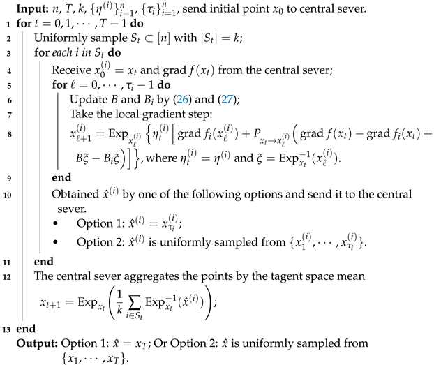 |
Inspired by the idea of SVRG-BB, we use the BB step size for RFedSVRG-2BB so that we can achieve the step size self-adjusting, which means we do not need to specify a step size for each client and therefore we maintain a faster speed of convergence. We call the new algorithm RFedSVRG-2BBS. We apply (23) to decide step length. Moreover, in order to make the convergence curve flatter in numerical experiments, we use the bounds for the step size. This method of calculating the step size is shown in (29) and (30).
RFedSVRG-2BBS: in Input of Algorithm 1 is replaced by , where . If , , in line 8 in Algorithm 1 is changed to
where
, and is calculated by (21) and (22). Else, .
4. Convergence Analysis
In this section, we present the convergence results with their convergence rate of RFedSVRG-2BB and RFedSVRG-2BBS. Before the convergence results are given, we will give some necessary conclusions and assumptions.
Assumption 1
(Smoothness). Suppose that is -smooth on the manifold. It implies that f is L-smooth with .
Denote , and in (21), (22) and (25). If the function f is L-smooth, . Similarly, . Then we can obtain the upper bound of and :
For RFedSVRG-2BBS, we can obtain the lower bound of in (30):
It means . If , from (30) we can see that is fixed. To avoid this situation, we should set . In this case, we have
Moreover, we have
For RFedSVRG-2BB and RFedSVRG-2BBS, B and are computed in (26) and (27), and we can obtain and
Assumption 2
(Regularization over manifold). The manifold is complete and there exists a compact set, , with diameter bounded by D so that all the iterates of Algorithm 1 and the optimal points are contained in . The sectional curvature in is bounded in . Then we can obtain the following key constant, defined in [4,17], to capture manifold curvature:
Lemma 2
(Corollary 8 in [4]). If the Riemannian manifold, , satisfies Assumption 2, for any points , the update satisfies
Next, we provide convergence results with their convergence rate for RFedSVRG-2BB and RFedSVRG-2BBS with the -strongly g-convex objective function. The proof is inspired from [17]. For the calculation of the convergence rate, we refer to [4].
Lemma 3
(-strongly g-convex, RFedSVRG-2BB and RFedSVRG-2BBS with ). Consider RFedSVRG-2BB and RFedSVRG-2BBS with Option 1 in each inner loop to obtain (line 10 in Algorithm 1) and take . Assumptions 1 and 2 are satisfied and f is μ-strongly g-convex in problem (1). Denote
Then we have .
Proof.
Denote and
Taking the expectation with respect to i in the t-th outer loop, we have and then we can bound the squared norm of as follows
where the first inequality is due to , the second inequality is due to and (33), the third inequality due to Assumption 1 is satisfied, the fourth inequality is due to , and the fifth inequality and third equality are due to .
Note that and , therefore
The first inequality uses Lemma 2 and the second one is due to (36). The third and fourth inequalities use the -strongly g-convexity of .
Denote , and . Since , . Note that , i.e., and from (37) we have , i.e., . Hence, we have and
Denoting
from inequation (38) we obtain . □
Theorem 1
(-strongly g-convex, RFedSVRG-2BB with ). Consider RFedSVRG-2BB with Option 1 in each inner loop to obtain (line 10 in Algorithm 1) and take . Assumptions 1 and 2 are satisfied and f is μ-strongly g-convex in problem (1). Take , we have
Denoting
and is the optimal point, the Output of Option 1 in RFedSVRG-2BB has linear convergence in expectation:
In this case, the convergence rate of RFedSVRG-2BB is .
Proof.
Since , without loss generality, we denote i as the client that we choose at the t-th outer loop. From Lemma 3, we know that , where is from (35). Because in RFedSVRG-2BB, we have , where is independent from t and denoted as
Since , we can obtain
Therefore for ,
Denoting , we obtain . Therefore, for all outer loops, t, we have . It follows directly from the algorithm after T outer loops,
By using the L-smooth of f and Assumption 2, we can obtain
Summing the above inequation over , we have
Therefore, the convergence rate of RFedSVRG-2BB is . □
Theorem 2
(-strongly g-convex, RFedSVRG-2BBS with ). Consider RFedSVRG-2BBS with Option 1 in each inner loop to obtain (line 10 in Algorithm 1) and take . Assumptions 1 and 2 are satisfied and f is μ-strongly g-convex in problem (1). For , take , we have
the Output of Option 1 in RFedSVRG-2BBS has linear convergence in expectation:
In this case, the convergence rate of RFedSVRG-2BBS is .
Proof.
Since , without loss of generality, we denote i as the client that we choose at the t-th iteration. From Lemma 3, we know that , where is from (35). Because , we have
From the fact that in RFedSVRG-2BBS, we can obtain , where is a constant that is independent from t and i and denoted as
Hence, we obtain the upper bound of :
For each outer loop, t, it holds that , It follows directly from the algorithm after T outer loops,
By using the L-smooth of f and Assumption 2, we can obtain
Summing the above inequation over , we have
Therefore, the convergence rate of RFedSVRG-2BBS is . □
Later, we show the convergence results of RFedSVRG-2BB and RFedSVRG-2BBS with . The conditions for conclusions do not need the objective function, f, to be g-convex.
Lemma 4
(Non-convex, RFedSVRG-2BB and RFedSVRG-2BBS with ). Suppose the problem (1) satisfies Assumptions 1 and 2. If we run RFedSVRG-2BB and RFedSVRG-2BBS with Option 1 in each inner loop to obtain and , we have
Proof.
From the local update in RFedSVRG-2BB and RFedSVRG-2BBS, we know that
where . Because , for , and , we have
Using the L-smooth of and the aggregation step (line 12 in Algorithm 1), we have
□
Theorem 3
(Non-convex, RFedSVRG-2BB with ). Suppose the problem (1) satisfies Assumptions 1 and 2. If we run RFedSVRG-2BB with Option 1 in in each inner loop to obtain , and , we have
Proof.
Theorem 4
(Non-convex, RFedSVRG-2BBS with ). Suppose the problem (1) satisfies Assumptions 1 and 2. If we run RFedSVRG-2BBS with Option 1 in in each inner loop to obtain , and , we have
Proof.
We also have the convergence results of RFedSVRG-2BB and RFedSVRG-2BBS with and . The results show that, when the objective function is only L-smooth, the algorithms can achieve sublinear convergence. Before giving the result we need the following lemma, which is inspired from [3,17].
Lemma 5
(Non-convex, RFedSVRG-2BB and RFedSVRG-2BBS). Suppose the problem (1) satisfies Assumptions 1 and 2. Denote i as the client we choose at the t-th outer loop in RFedSVRG-2BB and RFedSVRG-2BBS, is a free constant and
where and satisfy:
The square of the norm of at iterate has the upper bound:
Proof.
Denote , because f is L-smooth, we have
where the first inequality is due to f being L-smooth, the first equality is due to and , and the second equality is due to . Then the following inequality holds:
where the first inequality follows from Lemma 2 and the second inequality is due to , where is a free constant. Denote , where is a parameter that varies with ℓ. Substituting (45) and (46) into , we can obtain the following bound:
Denoting , we have
and
where the first inequality is due to , the second inequality is due to and (33) and the third inequality follows from Assumption 1. Substituting (48) into (47), we obtain
From inequation (49), we can obtain , , and
□
Theorem 5
(Non-convex, RFedSVRG-2BB with ). Suppose the problem (1) satisfies Assumptions 1 and 2. Consider RFedSVRG-2BB with Option 2 in each inner loop to obtain , if we set , and , where , and , the Output with Option 2 in RFedSVRG-2BB satisfies:
When the function f is h-gradient dominated, the convergence rate of RFedSVRG-2BB is
Proof.
Since , without loss of generality, we denote i as the client that we choose at the t-th outer loop. We take in (43), where . Because in RFedSVRG-2BB, , recursively from (42), it can be seen that:
where is a parameter and is a set of decreasing numbers.
Note that , which means that , then the upper bound of satisfies . Therefore, the lower bound of in (43) is:
Note that this lower bound, , is independent from the choice of the client, i. From (41), we have and
Because and we choose Option 2 in each inner loop to obtain , summing (44) over , we have
Summing the above inequation over , we obtain
Therefore, we have
When the function f is h-gradient dominated, we have . From (51), L-smooth of f and Assumption 2, we have
Therefore, the convergence rate of RFedSVRG-2BB is . □
Theorem 6
(Non-convex, RFedSVRG-2BBS with ). Suppose the problem (1) satisfies Assumptions 1 and 2. Consider RFedSVRG-2BBS with Option 2 in each inner loop to obtain , if we set , and , the Output with Option 2 in RFedSVRG-2BBS satisfies:
When the function f is h-gradient dominated, the convergence rate of RFedSVRG-2BBS is .
Proof.
Since , without loss of generality, we denote i as the client that we choose at the t-th outer loop. In RFedSVRG-2BB, , by recursive (42), we obtain , where is a parameter and is a series of decreasing numbers.
We fixed in (42), then we have and
Because , . From , we have
Then we can obtain the lower bound of , where is calculated from (43):
where the last inequality is due to (32). Note that the lower bound, , is independent from the choice of the client, i.
From (41), we have and . Because we choose Option 2 in each inner loop to obtain , summing (44) over , we obtain
Summing (52) over , we have
Therefore, we have
When the function f is h-gradient dominated, we have . From (53), L-smooth of f and Assumption 2, we have
Therefore, the convergence rate of RFedSVRG-2BBS is . □
Based on the theorems in this section, we briefly summarize the convergence rates of our algorithms when function f satisfies different properties in Table 1. For more details, please refer to the corresponding theorem and its proof.

Table 1.
This table summarizes the convergence rates we have proved for our algorithms. Where T is total number of communication of algorithms, L is the Lipschitz constant of f and D is the diameter of the domain in Assumption 2. For the conditions that need to be met and other parameter sources, please refer to the corresponding theorem.
5. Numerical Experiments
In this section, we will demonstrate the performance of RFedSVRG-2BB and RFedSVRG-2BBS in solving problem (1) and compare it with RFedSVRG [3], RFedAvg [3] and RFedProx [3]. We use the Pymanopt package [46]. Since the inverse of exponential mapping (logarithm mapping) on the Stiefel manifold is not easy to calculate, we use the projection-like retraction [47] and its inverse [48] to approximate the exponential mapping and the logarithm mapping, respectively.
We test the five algorithms on the PSD Karcher mean (2), PCA (3) and kPCA (4) on synthetic or real datasets. For all problems, we measure the norm of the global Riemannian gradients. Because the optimal solution of in problem (4) only represents the eigen-space corresponding to the r-largest eigenvalues, we also measure the principal angles [3,49] between the subspaces for kPCA.
5.1. Experiments on Synthetic Data
In this section, we demonstrate the results of the five algorithms for solving PCA (3) and the PSD Karcher mean (2) on synthetic data. We first generate the data , whose row vectors are generated from standard normal distribution. The in (3) and (2) are set to
Under these experiments, the datas in different agents are homogeneous in distribution, which provides a milder environment for comparing the behavior of all the algorithms. All algorithms iterate through the same random initial point. We terminate the algorithms if they meet one of the following conditions:
- (a)
- (b)
- the communication exceeds the specified number of rounds.
The y-axis of the figures in this subsection denotes and the x-axis denotes the outer loop in the algorithms, i.e., the round of communication in Federated Learning.
5.1.1. Experiments on PSD Karcher Mean
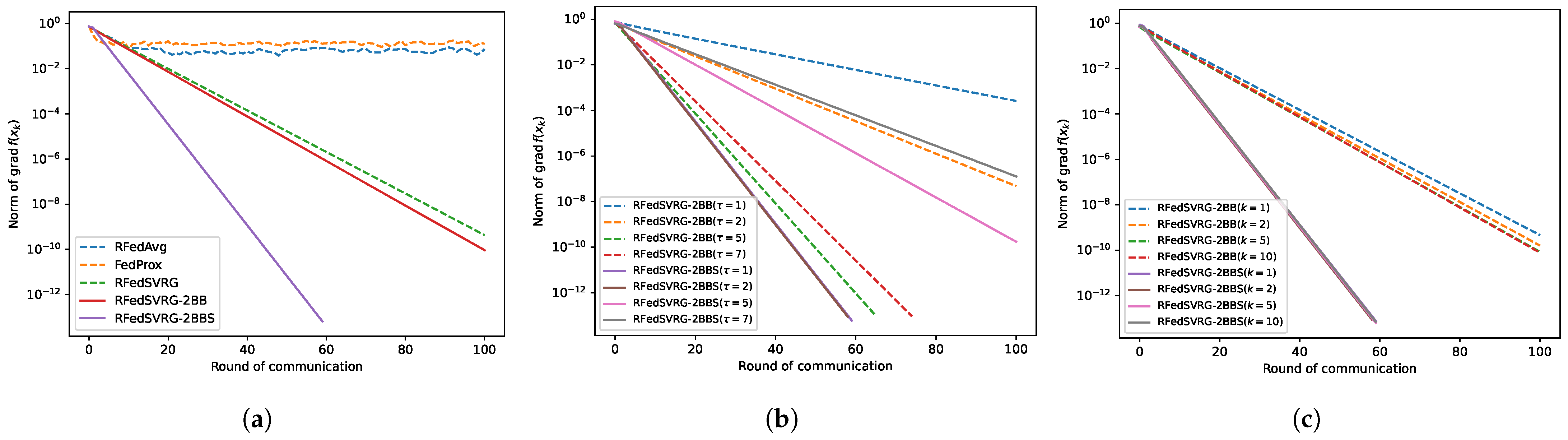
In this subsection, we test RFedAvg, RFedProx, RFedSVRG and RFedSVRG-BB to solve the PSD Karcher mean (2). In these experiments, we set in (54), and . For RFedAvg, RFedProx, RFedSVRG and RFedSVRG-2BB, we set . We set for RFedSVRG-2BBS. The results are given in Figure 1. The convergence curves of RFedSVRG-2BB and RFedSVRG-2BBS in Figure 1a–c show a linear rate of convergence, largely due to the fact that (2) is strongly geodesic convex [4].
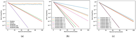
Figure 1.
Results for PSD Karcher mean problem (2). (a) is the comparison of the five algorithms with to reduce . (b) is the comparison of different in RFedSVRG-2BB and RFedSVRG-2BBS with . (c) is the comparison of different k in RFedSVRG-2BB and RFedSVRG-2BBS with .
From Figure 1a, we can see that RFedAvg and RFedProx are unable to reduce the norm of the Riemannian gradient to an acceptable level. RFedSVRG-2BB and RFedSVRG-2BBS can decrease the norm of the Riemannian gradient faster than RFedAvg, RFedProx and RFedSVRG, and RFedSVRG-2BBS is the fastest of all algorithms.
From Figure 1b, we can see that RFedSVRG-2BB and RFedSVRG-2BBS with different can convergence linearly. It is noted that the effect of taking is not as good as the effect of taking . The central idea in SVRG and its variants is that the stochastic gradients are used to estimate the change in the gradient between point and [2,29], and it is clear that, if and are close to each other, the variance of the estimate
line 8 of Algorithm 1 should be small, resulting in an estimate of with small variance. As the inner iterate proceeds further, variance grows, and the algorithms need to start a new outer loop to compute a new full gradient and reset the variance. Therefore it is important to set not too large to avoid a large variance.
From Figure 1c, the cases when RFedSVRG-2BB and RFedSVRG-2BBS with can decrease the norm of the Riemannian gradient in convergence can be seen. RFedSVRG-2BB with is able to reach a more acceptable level of the norm of the Riemannian gradient than RFedSVRG-2BB with .
5.1.2. Experiments on PCA
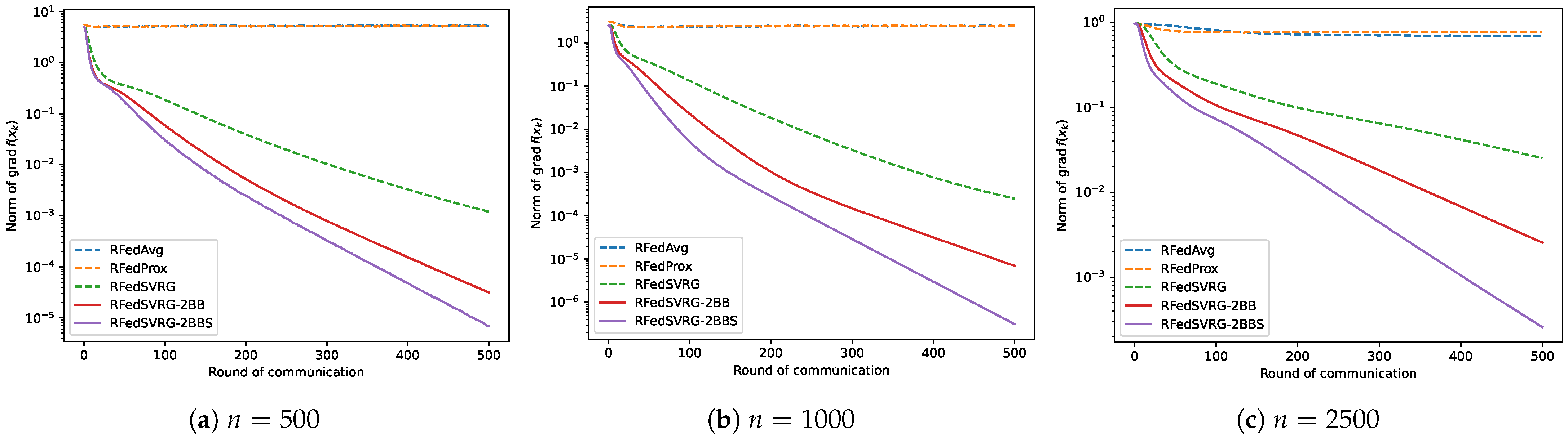
We now test the five algorithms on the standard PCA problem (3). In this test, we set the algorithms with different numbers of the agents, n, and pick up as the number of clients for each round. We partition the data sampled from 10,000 data points in into n agents on average, i.e., , in (54), and each of them contains equal numbers of data. The number of data in these experiments are relatively large. For all algorithms, we set . We use the constant step size for RFedAvg, RFedProx, RFedSVRG and RFedSVRG-2BB, and set for RFedSVRG-2BBS. We specify that the number of terminated rounds is 500. The results are given in Figure 2.
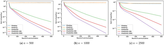
Figure 2.
Results for PCA (3).
From all the figures in Figure 2, we can see that RFedAvg and RFedProx are unable to reduce the norm of the Riemannian gradient to an acceptable level for different numbers of n. RFedSVRG-2BB and RFedSVRG-2BBS decrease the norm of the Riemannian gradient to a better level than RFedAvg, RFedProx and RFedSVRG with the same number of communications. Moreover, RFedSVRG-2BB and RFedSVRG-2BBS converge faster than RFedSVRG, and RFedSVRG-2BBS is the fastest.
5.2. Experiments on Real Data
In this subsection, we focus on the kPCA problem (4) here with four real datasets: the Iris dataset [50], the wine dataset [50], the breast cancer dataset [51] and the MNIST hand-written dataset [52]. They are highly heterogeneous real data and we use them to generate in problem (4).
We first normalize the four datasets. For one of the normalized datasets we denote it as , where each data sample, , in satisfies and m is the number of data in dataset . Then we randomly divide data in into n parts and denote the divided data as the dataset in clients. The covariance matrix, , in (4) is calculated as
Utilizing the features of (4), we can obtain the optimal point, , of (4) by directly solving the first r eigenvectors of i.e., if the the first r eigenvectors of A are , the optimal point, , in (4) is [5].
Then we can compute the principal angles between the iterate point, , and directly. Moreover, the Output, , of our algorithms is the projection matrix that could be used to extract the principal components of dataset by
which effectively reduces the dimension of data in from to , and D is a reduced dimensional dataset [5]. We randomly choose the initial point for each experiment and terminate the algorithms if they meet one of the following conditions:
- and the principal angle between and is less than ;
- the communication exceeds the specified number of rounds.
We present our results in Figure 3, Figure 4, Figure 5 and Figure 6. The x-axis of the figures denotes the round of communication in Federated Learning.
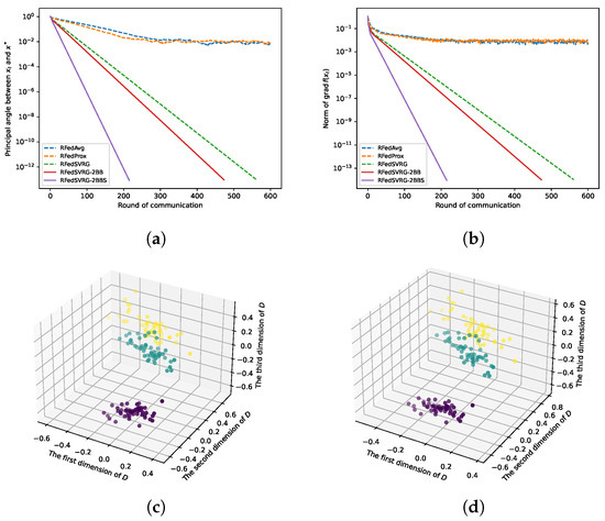
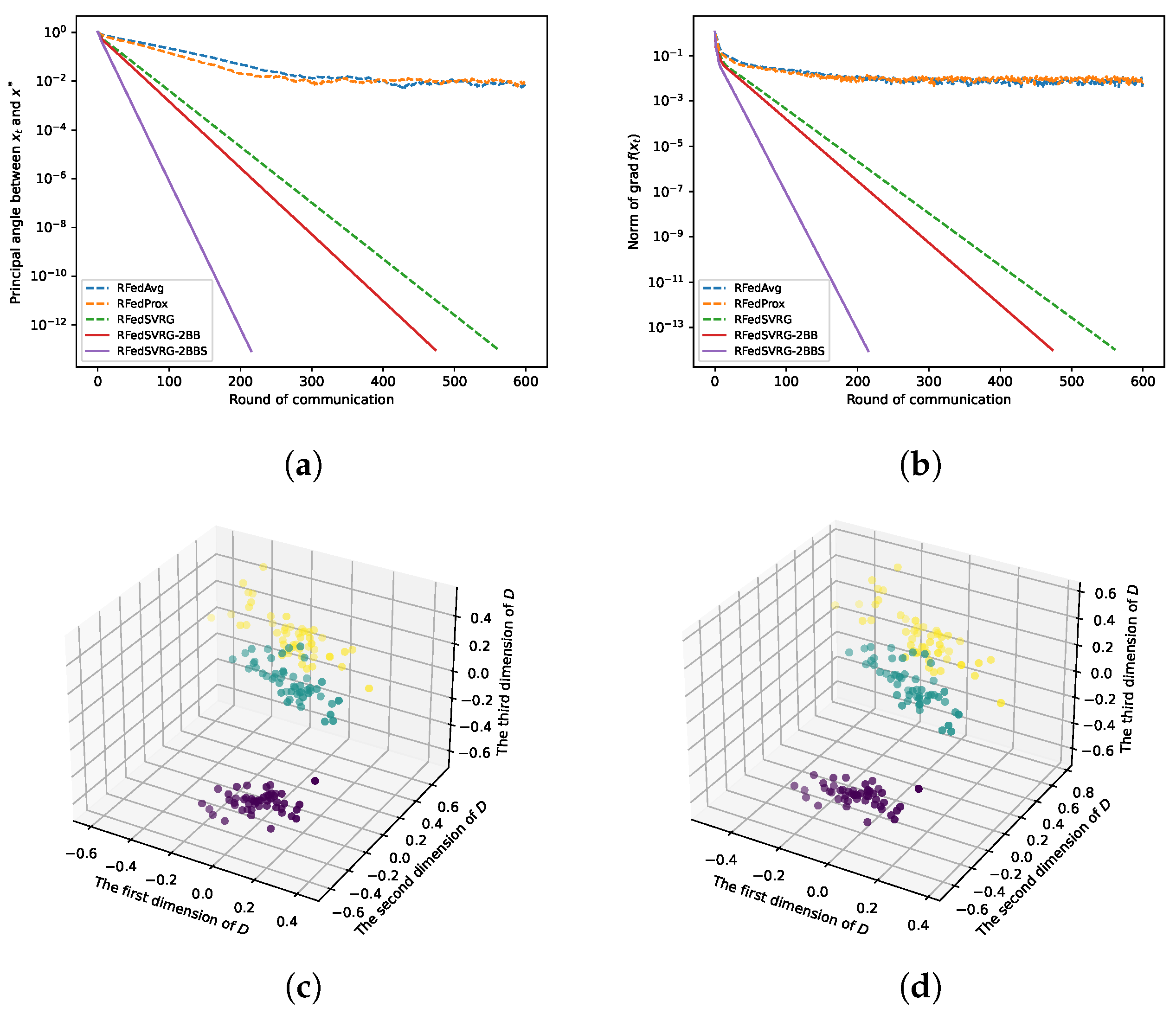
Figure 3.
Results for kPCA (4) with Iris dataset. The datas are in and we take , , and . We set for RFedSVRG-2BBS as and constant step size for RFedAvg, RFedProx, RFedSVRG and RFedSVRG-2BB. (a) Comparison of algorithms on reducing the principal angle between and . (b) Comparison of algorithms on reducing the norm of . (c) D in (55) for RFedSVRG-2BB. (d) D in (55) for RFedSVRG-2BBS.
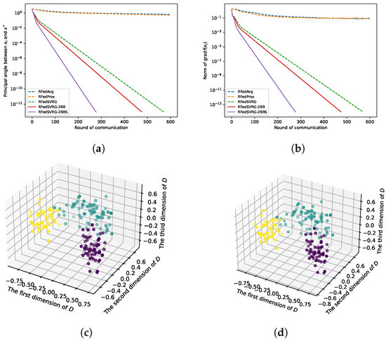
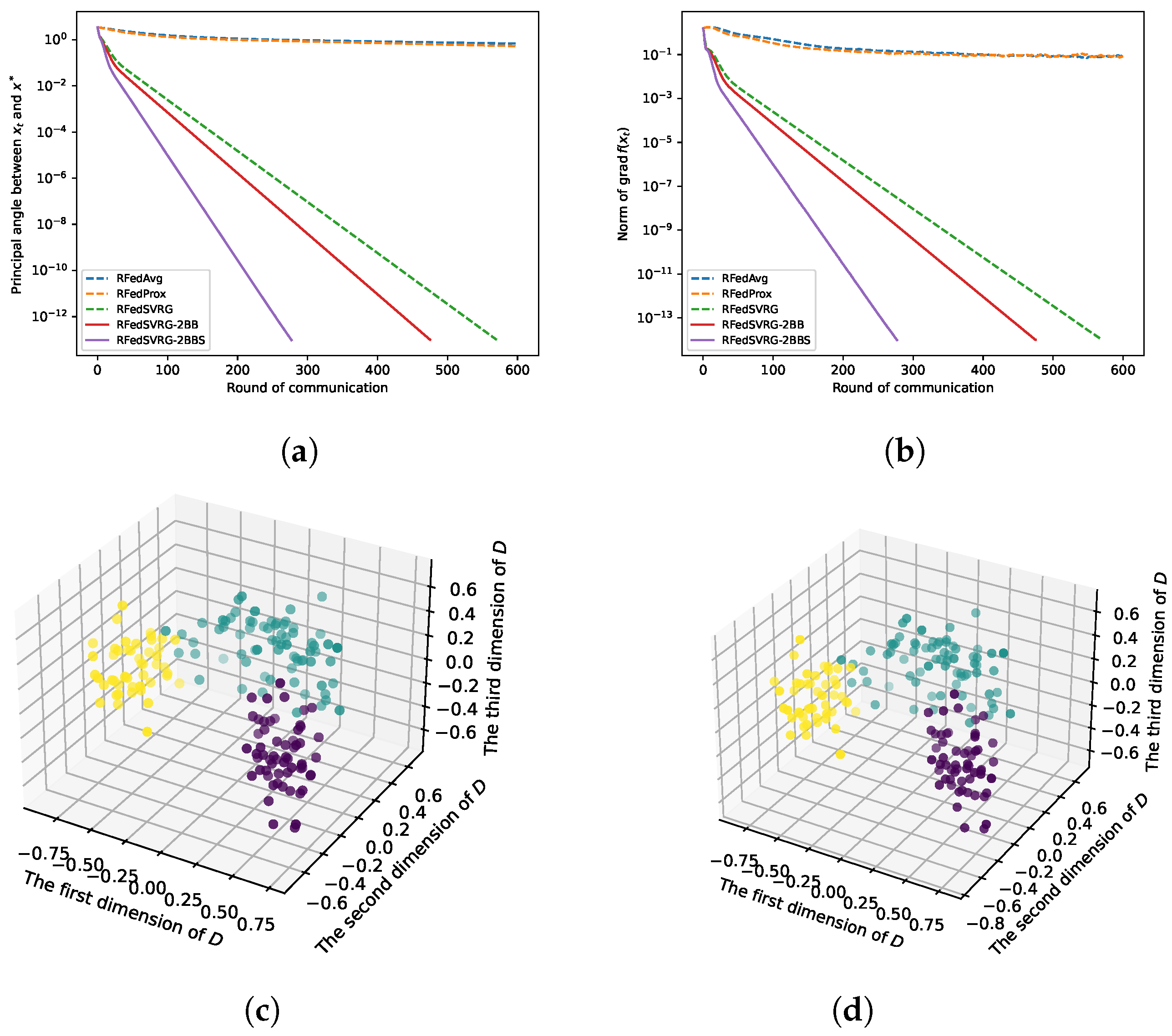
Figure 4.
Results for kPCA (4) with wine dataset. The datas are in and we take , , and . We set for RFedSVRG-BB as and constant step size for RFedAvg, RFedProx, RFedSVRG and RFedSVRG-2BB. (a) Comparison of algorithms on reducing the principal angle between and . (b) Comparison of algorithms on reducing the norm of . (c) D in (55) for RFedSVRG-2BB. (d) D in (55) for RFedSVRG-2BBS.
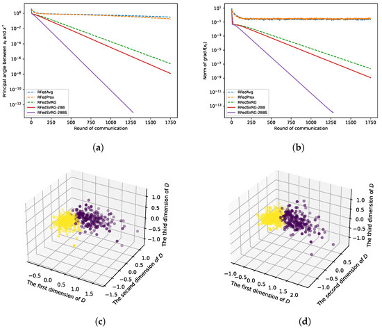
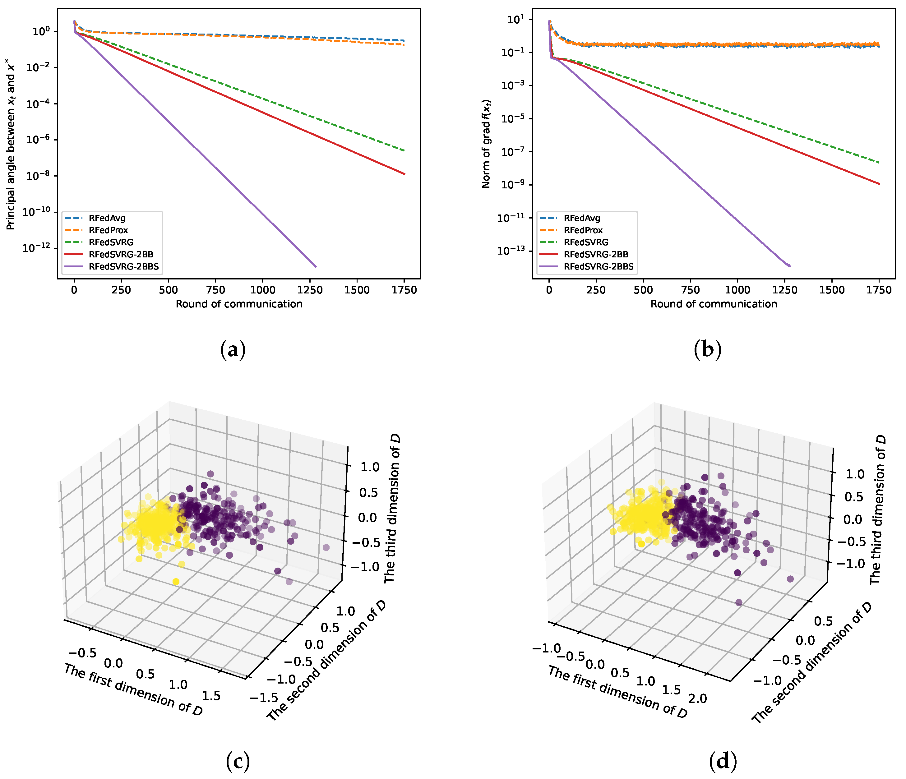
Figure 5.
Results for kPCA (4) with breast cancer dataset. The datas are in and we take , , and . We set for RFedSVRG-BB as and constant step size for RFedAvg, RFedProx, RFedSVRG and RFedSVRG-2BB. (a) Comparison of algorithms on reducing the principal angle between and . (b) Comparison of algorithms on reducing the norm of . (c) D in (55) for RFedSVRG-2BB. (d) D in (55) for RFedSVRG-2BBS.
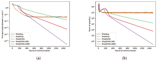
Figure 6.
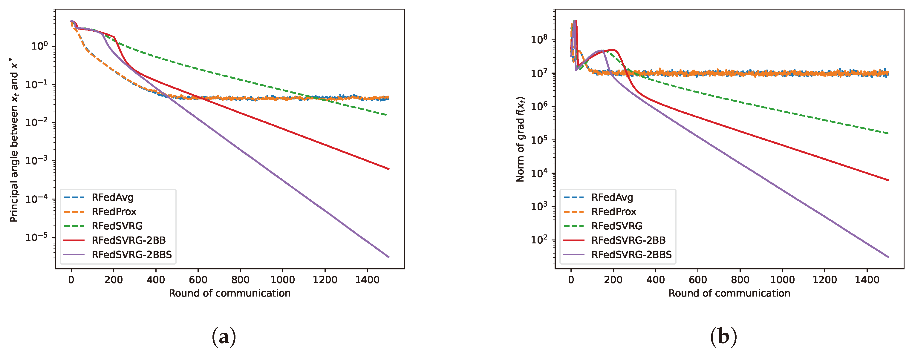
Results for kPCA (4) with MNIST hand-written dataset. The datas are in and we take , , and , respectively, for this experiment. We set for RFedSVRG-BB as and constant step size for RFedAvg, RFedProx and RFedSVRG as [3] recommended. (a) Comparison of algorithms on reducing the principal angle between and . (b) Comparison of algorithms on reducing the norm of .
In Figure 3a, Figure 4a, Figure 5a and Figure 6a, we plot the principal angle between and as the round of communication increases, i.e., the y-axis of the figures denotes the value of the principal angle between and . We can observe that RFedAvg and RFedProx are unable to reduce the principal angle between and to an acceptable level. RFedSVRG-2BB and RFedSVRG-2BBS are able to effectively decrease the principal angle. Comparing the five algorithms, RFedSVRG-2BB and RFedSVRG-2BBS have a faster convergence rate and RFedSVRG-2BBS is the fastest.
In Figure 3b, Figure 4b, Figure 5b and Figure 6b, we plot the norm of gradient of as the round of communication increases, i.e., the y-axis of the figures denotes . We can observe that RFedAvg and RFedProx are unable to reduce the norm of the Riemannian gradient to an acceptable level. RFedSVRG-2BB and RFedSVRG-2BBS are able to effectively decrease the norm of gradient of . Compared with RFedAvg, RFedProx and RFedSVRG, RFedSVRG-2BB and RFedSVRG-2BBS have a faster convergence rate and RFedSVRG-2BBS is the fastest.
In Figure 3c,d, Figure 4c,d and Figure 5c,d, because we take , we can draw the scatter plots for D in (55) in 3D space to obtain an intuitive feel, where in (55) is the output point of RFedSVRG-2BB and RFedSVRG-2BBS, respectively. The colors of points in Figure 3c,d, Figure 4c,d and Figure 5c,d are based on the label of the original datasets. It shows that the algorithms indeed grasp the principal direction of the datasets and effectively reduce the dimensionality of the datasets.
6. Conclusions
In this paper we applied the BB technique to approximate the second-order information in RFedSVRG and obtain a new Riemannian FL algorithm, RFedSVRG-2BB. Then we incorporated the BB step size for RFedSVRG-2BB as a new variant, RFedSVRG-2BBS. We analyzed the RFedSVRG-2BB and RFedSVRG-2BBS convergence rates for a strongly geodesically convex function and L-smooth non-convex function. Additionally, we conducted some numerical experiments on synthetic and real datasets. The results show that our algorithms are better than RFedSVRG and also outperform RFedAvg and RFedProxk, which are widely applied algorithms. Therefore, the RFedSVRG-2BB and RFedSVRG-2BBS methods can be regarded as competitive alternatives to the classic methods of solving Federated Learning problems.
Author Contributions
Conceptualization, H.X. and T.Y.; methodology, H.X.; software, H.X.; validation, H.X., T.Y. and K.W.; formal analysis, H.X.; investigation, H.X.; resources, T.Y.; writing—original draft preparation, H.X.; writing—review and editing, H.X.; visualization, H.X.; supervision, T.Y.; project administration, T.Y.; funding acquisition, T.Y. All authors have read and agreed to the published version of the manuscript.
Funding
This work was supported by the National Natural Science Foundation of China (Grant No. 11671205).
Data Availability Statement
Data is contained within the article.
Conflicts of Interest
The authors declare no conflict of interest.
References
- McMahan, B.; Moore, E.; Ramage, D.; Hampson, S.; Arcas, B.A.y. Communication-Efficient Learning of Deep Networks from Decentralized Data. In Proceedings of the 20th International Conference on Artificial Intelligence and Statistics, Fort Lauderdale, FL, USA, 20–22 April 2017; PMLR: New York, NY, USA, 2017; Volume 54, pp. 1273–1282. [Google Scholar]
- Konecný, J.; McMahan, H.; Ramage, D.; Richtárik, P. Federated Optimization: Distributed Machine Learning for On-Device Intelligence. arXiv 2016, arXiv:1610.02527. [Google Scholar]
- Li, J.; Ma, S. Federated Learning on Riemannian Manifolds. Appl. Set-Valued Anal. Optim. 2023, 5, 213–232. [Google Scholar]
- Zhang, H.; Sra, S. First-order Methods for Geodesically Convex Optimization. In Proceedings of the 29th Annual Conference on Learning Theory, New York, New York, USA, 23–26 June 2016; PMLR: New York, NY, USA, 2016; Volume 49, pp. 1617–1638. [Google Scholar]
- Härdle, W.; Simar, L. Applied Multivariate Statistical Analysis; Springer: Cham, Switzerland, 2019. [Google Scholar]
- Cheung, Y.; Lou, J.; Yu, F. Vertical Federated Principal Component Analysis on Feature-Wise Distributed Data. In Web Information Systems Engineering, Proceedings of the 22nd International Conference on Web Information Systems Engineering, WISE 2021, Melbourne, VIC, Australia, 26–29 October 2021; WISE: Cham, Switzerland, 2021; pp. 173–188. [Google Scholar]
- Boumal, N.; Absil, P.A. Low-rank matrix completion via preconditioned optimization on the Grassmann manifold. Linear Algebra Its Appl. 2015, 475, 200–239. [Google Scholar] [CrossRef]
- Pennec, X.; Fillard, P.; Ayache, N. A Riemannian Framework for Tensor Computing. Int. J. Comput. Vis. 2005, 66, 41–66. [Google Scholar] [CrossRef]
- Fletcher, P.; Joshi, S. Riemannian geometry for the statistical analysis of diffusion tensor data. Signal Process. 2007, 87, 250–262. [Google Scholar] [CrossRef]
- Rentmeesters, Q.; Absil, P. Algorithm comparison for Karcher mean computation of rotation matrices and diffusion tensors. In Proceedings of the 19th European Signal Processing Conference, Barcelona, Spain, 29 August–2 September 2011; pp. 2229–2233. [Google Scholar]
- Cowi, S.; Yang, G. Averaging anisotropic elastic constant data. J. Elast. 1997, 46, 151–180. [Google Scholar]
- Massart, E.; Chevallier, S. Inductive Means and Sequences Applied to Online Classification of EEG. In Geometric Science of Information, Proceedings of the Third International Conference, GSI 2017, Paris, France, 7–9 November 2017; Springer International Publishing: Berlin/Heidelberg, Germany, 2017; pp. 763–770. [Google Scholar]
- Magai, G. Deep Neural Networks Architectures from the Perspective of Manifold Learning. In Proceedings of the 2023 IEEE 6th International Conference on Pattern Recognition and Artificial Intelligence (PRAI), Haikou, China, 18–20 August 2023; pp. 1021–1031. [Google Scholar]
- Yerxa, T.; Kuang, Y.; Simoncelli, E.; Chung, S. Learning Efficient Coding of Natural Images with Maximum Manifold Capacity Representations. In Proceedings of the Advances in Neural Information Processing Systems; Oh, A., Naumann, T., Globerson, A., Saenko, K., Hardt, M., Levine, S., Eds.; Curran Associates, Inc.: New Orleans, LA, USA, 2023; Volume 36, pp. 24103–24128. [Google Scholar]
- Chen, S.; Ma, S.; Man-Cho So, A.; Zhang, T. Proximal Gradient Method for Nonsmooth Optimization over the Stiefel Manifold. SIAM J. Optim. 2020, 30, 210–239. [Google Scholar] [CrossRef]
- Boumal, N. An Introduction to Optimization on Smooth Manifolds; Cambridge University Press: Cambridge, UK, 2022. [Google Scholar]
- Zhang, H.; Reddi, S.; Sra, S. Riemannian svrg: Fast stochastic optimization on riemannian manifolds. Adv. Neural Inf. Process. Syst. 2016, 29, 4599–4607. [Google Scholar]
- Li, T.; Sahu, A.K.; Zaheer, M.; Sanjabi, M.; Talwalkar, A.; Smith, V. Federated Optimization in Heterogeneous Networks. Proc. Mach. Learn. Syst. 2020, 2, 429–450. [Google Scholar]
- Pathak, R.; Wainwright, M. FedSplit: An algorithmic framework for fast federated optimization. Adv. Neural Inf. Process. Syst. 2020, 33, 7057–7066. [Google Scholar]
- Wang, J.; Liu, Q.; Liang, H.; Joshi, G.; Poor, H.V. Tackling the objective inconsistency problem in heterogeneous federated optimization. In Proceedings of the 34th International Conference on Neural Information Processing Systems, NIPS ’20, Vancouver, BC, Canada, 6–12 December 2020; Curran Associates, Inc.: Red Hook, NY, USA, 2020. [Google Scholar]
- Mitra, A.; Jaafar, R.; Pappas, G.; Hassani, H. Linear Convergence in Federated Learning: Tackling Client Heterogeneity and Sparse Gradients. Adv. Neural Inf. Process. Syst. 2021, 34, 14606–14619. [Google Scholar]
- Karimireddy, S.P.; Kale, S.; Mohri, M.; Reddi, S.J.; Stich, S.U.; Suresh, A.T. SCAFFOLD: Stochastic controlled averaging for federated learning. In Proceedings of the 37th International Conference on Machine Learning, ICML’20, Virtual Event, 13–18 July 2020. [Google Scholar]
- Yuan, H.; Zaheer, M.; Reddi, S. Federated Composite Optimization. In Proceedings of the Machine Learning Research, 38th International Conference on Machine Learning, 18–24 July 2021; Meila, M., Zhang, T., Eds.; PMLR: New York, NY, USA, 2021; Volume 139, pp. 12253–12266. [Google Scholar]
- Bao, Y.; Crawshaw, M.; Luo, S.; Liu, M. Fast Composite Optimization and Statistical Recovery in Federated Learning. In Proceedings of the Machine Learning Research, 39th International Conference on Machine Learning, Baltimore, MD, USA, 17–23 July 2022; Chaudhuri, K., Jegelka, S., Song, L., Szepesvari, C., Niu, G., Sabato, S., Eds.; PMLR: New York, NY, USA, 2022; Volume 162, pp. 1508–1536. [Google Scholar]
- Tran Dinh, Q.; Pham, N.H.; Phan, D.; Nguyen, L. FedDR–Randomized Douglas-Rachford Splitting Algorithms for Nonconvex Federated Composite Optimization. Neural Inf. Process. Syst. 2021, 34, 30326–30338. [Google Scholar]
- Zhang, J.; Hu, J.; Johansson, M. Composite Federated Learning with Heterogeneous Data. In Proceedings of the ICASSP 2024—2024 IEEE International Conference on Acoustics, Speech and Signal Processing (ICASSP), Seoul, Republic of Korea, 14–19 April 2023; pp. 8946–8950. [Google Scholar]
- Zhang, J.; Hu, J.; So, A.M.; Johansson, M. Nonconvex Federated Learning on Compact Smooth Submanifolds With Heterogeneous Data. arXiv 2024, arXiv:2406.08465. [Google Scholar] [CrossRef]
- Charles, Z.; Konečný, J. Convergence and Accuracy Trade-Offs in Federated Learning and Meta-Learning. In Proceedings of the 24th International Conference on Artificial Intelligence and Statistics, Virtual, 13–15 April 2021; Banerjee, A., Fukumizu, K., Eds.; PMLR: New York, NY, USA, 2021; Volume 130, pp. 2575–2583. [Google Scholar]
- Johnson, R.; Zhang, T. Accelerating stochastic gradient descent using predictive variance reduction. In Proceedings of the 26th International Conference on Neural Information Processing Systems, NIPS’13, Lake Tahoe, NV, USA, 5–10 December 2013; Curran Associates Inc.: Red Hook, NY, USA, 2013; Volume 1, pp. 315–323. [Google Scholar]
- Huang, Z.; Huang, W.; Jawanpuria, P.; Mishra, B. Federated Learning on Riemannian Manifolds with Differential Privacy. arXiv 2024, arXiv:2404.10029. [Google Scholar]
- Nguyen, T.A.; Le, L.T.; Nguyen, T.D.; Bao, W.; Seneviratne, S.; Hong, C.S.; Tran, N.H. Federated PCA on Grassmann Manifold for IoT Anomaly Detection. IEEE/ACM Trans. Netw. 2024, 1–16. [Google Scholar] [CrossRef]
- Gower, R.; Le Roux, N.; Bach, F. Tracking the gradients using the Hessian: A new look at variance reducing stochastic methods. In Proceedings of the Machine Learning Research, Twenty-First International Conference on Artificial Intelligence and Statistics, Playa Blanca, Lanzarote, Spain, 9–11 April 2018; Storkey, A., Perez-Cruz, F., Eds.; PMLR: New York, NY, USA, 2018; Volume 84, pp. 707–715. [Google Scholar]
- Tankaria, H.; Yamashita, N. A stochastic variance reduced gradient using Barzilai-Borwein techniques as second order information. J. Ind. Manag. Optim. 2024, 20, 525–547. [Google Scholar] [CrossRef]
- Roux, R.; Schmidt, M.; Bach, F. A Stochastic Gradient Method with an Exponential Convergence Rate for Finite Training Sets. In Proceedings of the 25th International Conference on Neural Information Processing Systems, NIPS’12, Lake Tahoe, NV, USA, 3–6 December 2012; Curran Associates Inc.: Red Hook, NY, USA, 2012; Volume 2, pp. 2663–2671. [Google Scholar]
- Tan, C.; Ma, S.; Dai, Y.; Qian, Y. Barzilai-Borwein step size for stochastic gradient descent. In Proceedings of the 30th International Conference on Neural Information Processing Systems, NIPS’16, Barcelona, Spain, 5–10 December 2016; Curran Associates Inc.: Red Hook, NY, USA, 2016; pp. 685–693. [Google Scholar]
- Barzilai, J.; Borwein, J. Two-Point Step Size Gradient Methods. IMA J. Numer. Anal. 1988, 8, 141–148. [Google Scholar] [CrossRef]
- Francisco, J.; Bazán, F. Nonmonotone algorithm for minimization on closed sets with applications to minimization on Stiefel manifolds. J. Comput. Appl. Math. 2012, 236, 2717–2727. [Google Scholar] [CrossRef]
- Jiang, B.; Dai, Y. A framework of constraint preserving update schemes for optimization on Stiefel manifold. Math. Program. 2013, 153, 535–575. [Google Scholar] [CrossRef]
- Wen, Z.; Yin, W. A feasible method for optimization with orthogonality constraints. Math. Program. 2013, 142, 397–434. [Google Scholar] [CrossRef]
- Iannazzo, B.; Porcelli, M. The Riemannian Barzilai–Borwein method with nonmonotone line search and the matrix geometric mean computation. IMA J. Numer. Anal. 2017, 38, 495–517. [Google Scholar] [CrossRef]
- Absil, P.; Mahony, R.; Sepulchre, R. Optimization Algorithms on Matrix Manifolds; Princeton University Press: Princeton, NJ, USA, 2007. [Google Scholar]
- Lee, J.M. Introduction to Riemannian Manifolds, 2nd ed.; Springer International Publishing: Cham, Switzerland, 2018; pp. 225–262. [Google Scholar]
- Petersen, P. Riemannian Geometry; Springer: Berlin/Heidelberg, Germany, 2006; Volume 171. [Google Scholar]
- Tu, L. An Introduction to Manifolds; Springer: New York, NY, USA, 2011. [Google Scholar]
- Nocedal, J.; Wright, S. Numerical Optimization; Springer: New York, NY, USA, 1999. [Google Scholar]
- Townsend, J.; Koep, N.; Weichwald, S. Pymanopt: A Python Toolbox for Optimization on Manifolds using Automatic Differentiation. J. Mach. Learn. Res. 2016, 17, 4755–4759. [Google Scholar]
- Absil, P.; Malick, J. Projection-like Retractions on Matrix Manifolds. SIAM J. Optim. 2012, 22, 135–158. [Google Scholar] [CrossRef]
- Kaneko, T.; Fiori, S.; Tanaka, T. Empirical Arithmetic Averaging Over the Compact Stiefel Manifold. IEEE Trans. Signal Process 2013, 61, 883–894. [Google Scholar] [CrossRef]
- Zhu, P.; Knyazev, A. Angles between subspaces and their tangents. J. Numer. Math. 2013, 21, 325–340. [Google Scholar] [CrossRef]
- Forina, M.; Leardi, R.; Armanino, C.; Lanteri, S. PARVUS: An Extendable Package of Programs for Data Exploration. J. Chemom. 1990, 4, 191–193. [Google Scholar]
- Street, W.N.; Wolberg, W.H.; Mangasarian, O.L. Nuclear feature extraction for breast tumor diagnosis. In Proceedings of the Biomedical Image Processing and Biomedical Visualization, San Jose, CA, USA, 1–4 February 1993; Acharya, R.S., Goldgof, D.B., Eds.; International Society for Optics and Photonics, SPIE: Bellingham, WA, USA, 1993; Volume 1905, pp. 861–870. [Google Scholar]
- Lecun, Y.; Bottou, L.; Bengio, Y.; Haffner, P. Gradient-based learning applied to document recognition. Proc. IEEE 1998, 86, 2278–2324. [Google Scholar] [CrossRef]
Disclaimer/Publisher’s Note: The statements, opinions and data contained in all publications are solely those of the individual author(s) and contributor(s) and not of MDPI and/or the editor(s). MDPI and/or the editor(s) disclaim responsibility for any injury to people or property resulting from any ideas, methods, instructions or products referred to in the content. |
© 2024 by the authors. Licensee MDPI, Basel, Switzerland. This article is an open access article distributed under the terms and conditions of the Creative Commons Attribution (CC BY) license (https://creativecommons.org/licenses/by/4.0/).