Memory Effects in the Magnetohydrodynamic Axial Symmetric Flows of Oldroyd-B Fluids in a Porous Annular Channel

Abstract

In this article, we analytically investigate the isothermal magnetohydrodynamic axial symmetric flows of ordinary and fractional incompressible Oldroyd-B fluids through a porous medium in an annular channel. The fluid’s motion is generated by an outer cylinder, which moves along its symmetry axis with an arbitrary time-dependent velocity $Vh(t)$. Closed-form expressions are established for the dimensionless velocity fields of both kinds of fluids, generating exact solutions for any motion of this type. To illustrate the concept, two particular cases are considered, and the velocity fields corresponding to the flow induced by the outer cylinder are presented in simple forms, with the results validated graphically. The motion of fractional and ordinary fluids becomes steady over time, and their corresponding velocities are presented as the sum of their steady and transient components. Moreover, the steady components of these velocities are identical. The influence of magnetic fields and porous media on the flow of fractional fluids is graphically depicted and discussed. It was found that a steady state is reached earlier in the presence of a magnetic field and later in the presence of a porous medium. Moreover, this state is obtained earlier in fractional fluids compared with ordinary fluids.

1. Introduction

The constitutive equations of incompressible Oldroyd-B fluids (IOBFs) are given by the following relations [1]:

$$\mathit{T}=-p\mathit{I}+\mathit{S},\hspace{1em}\left(1+\lambda {\displaystyle \frac{\delta }{\delta t}}\right)\mathit{S}=\mu \left(1+{\lambda }_r{\displaystyle \frac{\delta }{\delta t}}\right)\mathit{A},$$

(1)

in which T is the Cauchy stress tensor; S is the extra-stress tensor; A is the first Rivlin–Ericksen tensor; I is the identity tensor; p is the hydrostatic pressure; $\mu$ is the dynamic viscosity; $\lambda$ and ${\lambda }_r$ are the relaxation and retardation times, respectively; and $\delta /\delta t$ denotes the upper-convected time derivative. If ${\lambda }_r=0$ or ${\lambda }_r=\lambda =0$, the governing Equations (1) define incompressible Maxwell or Newtonian fluids, respectively.

Oldroyd-B fluids exhibit the phenomenon known as viscoelasticity, namely, the ability of a material to behave as both a viscous fluid (with resistance to flow) and an elastic solid (able to recover its original shape after deformation). Recent studies have shown that Oldroyd-B fluids are essential in modeling the behavior of complex fluids such as polymer solutions, gels, and melts. They are also used in oil reservoirs and water filtration systems. The use of Oldroyd-B fluids in the design of medical devices like artificial hearts and blood pumps to replicate the behavior of blood flow in the human cardiovascular system is a significant part of the application of these fluids in the biomedical field.

Different exact solutions for the unsteady motion of these fluids in cylindrical domains were provided by Waters and King [2], Rajagopal and Bhatnagar [3], Wood [4], Fetecau [5], Fetecau et al. [6], McGinty et al. [7], Imran et al. [8], and Ullah et al. [9]. Some of them were extended to the motion of fractional fluids by Tong et al. [10,11], Qi and Jin [12], Kamran et al. [13], Mathur and Khandelwal [14], Riaz et al. [15], Ullah et al. [16], Sadiq et al. [17], and Madeeha Tahir et al. [18]. In the last three decades, fractional calculus has had much success in describing viscoelasticity. Governing equations with fractional derivatives proved to be a significant tool in describing the viscoelastic properties of many fluids. A good fit of the theoretical results with experimental data was found by Song and Jiang [19] and Makris [20] when using fractional models of some rate-type fluids. Bagley and Torvik [21], Friedrich [22], and Heibig and Palade [23] proposed constitutive equations with fractional derivatives that could describe the rheological behavior of viscoelastic materials. A historical perspective on the fractional calculus used in linear viscoelasticity and constitutive fractional modeling based on basic thermodynamic principles was provided in the papers by Mainardi [24] and Hristov [25], respectively.

The modeling of a fluid’s motion through a porous medium or in the presence of a magnetic field has many applications in agricultural engineering, the petroleum industry, MHD generators, plasma studies, nuclear reactors, polymer technology, geophysical and astrophysical studies, and so on. The interaction between a magnetic field and a moving electrical conducting fluid induces effects with important applications in chemistry, physics, and engineering, as well as the modeling of biological fluids, polymer manufacturing, and hydrology. Over time, many exact solutions have been established for the magnetohydrodynamic (MHD) flow of IOBFs through a porous medium in a rectangular domain, including those presented by Tan and Masuoka [26], Hussain et al. [27], Khan et al. [28], Hayat et al. [29], Khan and Ijaz [30], and Riaz et al. [31]. Unfortunately, there are very few solutions for the similar motion of fluids in cylindrical domains. However, some interesting results concerning their MHD motion through a porous medium in a cylindrical domain were obtained by Hayat et al. [32,33], Hamza [34], Fetecau et al. [35], Cao et al. [36], and Fetecau and Vieru [37]. The influence of a porous medium on the unsteady helical flows of fractional Oldroyd-B fluids among coaxial cylinders was realized by Ghazi and Waleed [38], but the results obtained from their governing equations, beginning with Equations (2) and (3) onwards, are wrong.

The purpose of this work is to provide exact general solutions for isothermal MHD axial flows of ordinary and fractional, electricity-conducting, incompressible Oldroyd-B fluids (ECIOBFs) through a porous medium between two infinite coaxial circular cylinders. The fluid motion is generated by the outer cylinder, which slides along its symmetry axis with an arbitrary time-dependent velocity. Closed-form general expressions, which are new to this field of research, are established for the fluid’s velocity, non-trivial shear stress, and Darcy’s resistance. These can generate exact solutions for any MHD motion of this kind for but ordinary and fractional fluids. To illustrate, two particular cases are considered, and the solutions obtained with respect to the motion induced by the cylinder are presented. Both the ordinary and fractional fluids’ motion becomes steady with time. Moreover, their steady velocity fields are identical. The time required to reach a steady state was graphically determined for the flow of fractional ECIOBFs. It was found that the steady state is obtained earlier in the presence of a magnetic field and later in the presence of a porous medium.

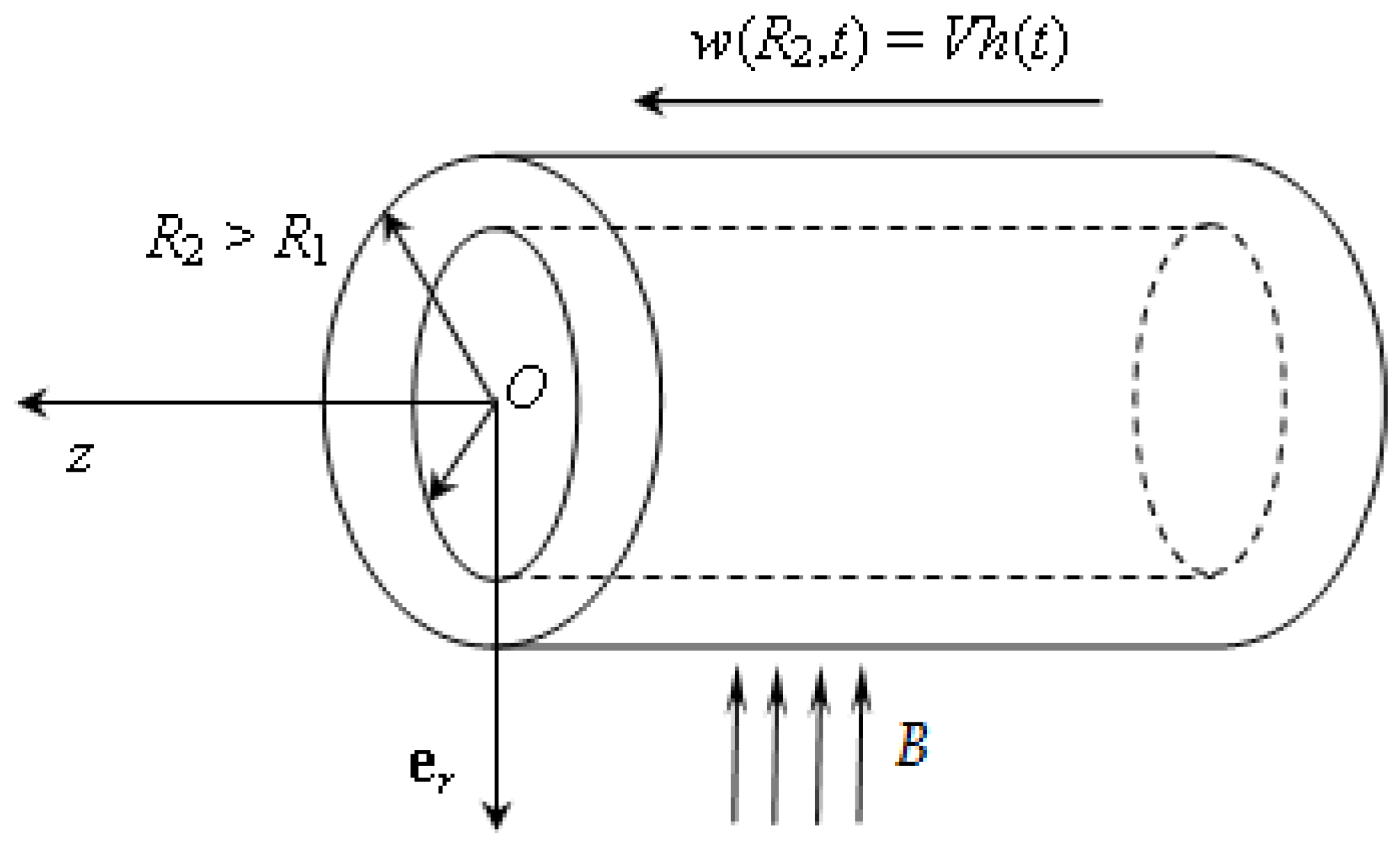
2. Statement of the Problem

Suppose that an electricity-conducting incompressible Oldroyd-B fluid (ECIOBF), whose constitutive equations are given by the relations in (1), is stationary in a porous medium between two infinite horizontal coaxial circular cylinders of radii $R_1$ and $R_2$ (>R₁), as in Figure 1.

After the moment $t=0^{+}$, the outer cylinder begins to slide along its axis with the time-dependent velocity $Vh(t)$, and a magnetic field of constant strength B acts perpendicular on the flow direction [33,34]. Here, V is a constant velocity, and the piecewise continuous function $h(\cdot )$ has its zero value in $t=0$. The fluid begins to move, and the corresponding velocity vector w has the form [33,34]

$$w=w(r,t)=\left(0,0,w(r,t)\right); R_1<r<R_2, t>0,$$

(2)

in the convenient cylindrical coordinate system r, $\theta$, and z. For such fluid motions, the continuity equation is identically satisfied.

Assuming that the extra-stress tensor S, as well as the velocity vector $w$, is a function of only r and t, it is not difficult to show that the non-null shear stress $\eta (r,t)=S_{rz}(r,t)$ has to satisfy the partial differential equation [33,34]

$$\left(1+\lambda {\displaystyle \frac{\partial }{\partial t}}\right)\eta (r,t)=\mu \left(1+{\lambda }_r{\displaystyle \frac{\partial }{\partial t}}\right){\displaystyle \frac{\partial w(r,t)}{\partial r}}; R_1<r<R_2, t>0.$$

(3)

We also suppose that the magnetic permeability of the fluid is constant, the imposed electric field is zero, and the induced magnetic field is negligible in comparison with the applied magnetic field. Under these conditions, and in the absence of a pressure gradient in the flow direction, the balance of linear momentum reduces to the partial differential equation [37]

$$\rho {\displaystyle \frac{\partial w(r,t)}{\partial t}}={\displaystyle \frac{\partial \eta (r,t)}{\partial r}}+{\displaystyle \frac{1}{r}}\eta (r,t)-\sigma B^{2}w(r,t)+R(r,t); R_1<r<R_2, t>0,$$

(4)

in which $\rho$ is the fluid density, $\sigma$ is the electrical conductivity, and the Darcy’s resistance $R(r,t)$ satisfies the partial differential equation

$$\left(1+\lambda {\displaystyle \frac{\partial }{\partial t}}\right)R(r,t)=-\mu {\displaystyle \frac{\phi }{k}}\left(1+{\lambda }_r{\displaystyle \frac{\partial }{\partial t}}\right)w(r,t); R_1<r<R_2, t>0.$$

(5)

where the constants $\phi$ ($0<\phi <1$) and k ($>0$) are the porosity and the permeability of porous medium.

Since the fluid is at rest up to the initial moment $t=0$,

$$w(r,0)=0, \eta (r,0)=0, R(r,0)=0; R_1<r<R_2.$$

(6)

The corresponding boundary conditions are

$$w(R_1,t)=0, w(R_2,t)=Vh(t); t\ge 0.$$

(7)

By introducing the following set of non-dimensional functions, variables, and parameters, we obtain the following:

$$\begin{array}{l} r^{*}={\displaystyle \frac{1}{R_2}}r, t^{*}={\displaystyle \frac{\nu }{R_2^2}}t, w^{*}={\displaystyle \frac{1}{V}}w, {\eta }^{*}={\displaystyle \frac{R_2}{\mu V}}\eta , R^{*}={\displaystyle \frac{R_2^2}{\mu V}}R,\\ h^{*}(t^{*})=h\left({\displaystyle \frac{R_2^2}{\nu }}{t}^{*}\right), \alpha ={\displaystyle \frac{\nu }{R_2^2}}\lambda , \beta ={\displaystyle \frac{\nu }{R_2^2}}{\lambda }_r,\end{array}$$

(8)

where $\nu =\mu /\rho$ is the kinematic viscosity of the fluid and, by abandoning the star notation, one finds the following dimensionless forms:

$$\left(1+\alpha {\displaystyle \frac{\partial }{\partial t}}\right)\eta (r,t)=\left(1+\beta {\displaystyle \frac{\partial }{\partial t}}\right){\displaystyle \frac{\partial w(r,t)}{\partial r}}; r_0<r<1, t>0,$$

(9)

$${\displaystyle \frac{\partial w(r,t)}{\partial t}}={\displaystyle \frac{\partial \eta (r,t)}{\partial r}}+{\displaystyle \frac{1}{r}}\eta (r,t)-Mw(r,t)+R(r,t)=0; r_0<r<1, t>0,$$

(10)

$$\left(1+\alpha {\displaystyle \frac{\partial }{\partial t}}\right)R(r,t)=-K\left(1+\beta {\displaystyle \frac{\partial }{\partial t}}\right)w(r,t); r_0<r<1, t>0,$$

(11)

of the governing Equations (3)–(5).

In the above equations, $r_0=R_1/R_2$ and the magnetic and porous parameters M and K, respectively, are defined by the following relations:

$$M={\displaystyle \frac{\sigma B^2}{\rho }}{\displaystyle \frac{R_2^2}{\nu }}= {\displaystyle \frac{R_2^2}{\mu }}\sigma B^2, K={\displaystyle \frac{\phi }{k}}{R}_2^2.$$

(12)

The corresponding dimensionless initial and boundary conditions are

$$w(r,0)=0, \eta (r,0)=0, R(r,0)=0; r_0<r<1,$$

(13)

$$w(r_0,t)=0, w(1,t)=h(t); t\ge 0.$$

(14)

In the next equation, for extension and to better incorporate memory effects into the behavior of the fluid, we also consider the corresponding fractional model characterized by the dimensionless governing Equation (10) and

$$\left(1+\alpha { }^C{D}_t^{\gamma }\right) \eta (r,t)=\left(1+\beta { }^C{D}_t^{\gamma }\right){\displaystyle \frac{\partial w(r,t)}{\partial r}}; r_0<r<1, t>0,$$

(15)

$$\left(1+\alpha { }^C{D}_t^{\gamma }\right)R(r,t)=-K\left(1+\beta { }^C{D}_t^{\gamma }\right)w(r,t); r_0<r<1, t>0.$$

(16)

The Caputo derivative of order $\gamma$ from the above relations is defined by the relation

$${}^{C}D_t^{\gamma }u(r,t)=\left\{\begin{array}{l}{\displaystyle \frac{1}{\Gamma (1-\gamma )}}{\displaystyle \underset{0}{\overset{t}{\int }}\frac{1}{{(t-\tau )}^{\gamma }}}{\displaystyle \frac{\partial u(r,\tau )}{\partial \tau }}d\tau if 0<\gamma <1,\\ {\displaystyle \frac{\partial u(r,t)}{\partial t}} if \gamma =1,\end{array}\right.$$

(17)

in which $\Gamma (\cdot )$ is the Gamma function. Inserting $\gamma =1$ into Equations (15) and (16), one recovers the governing Equations (9) and (11), which correspond to motion of ordinary ECIOBFs.

The Laplace and finite Hankel transforms will be used to generate solutions for the systems of the partial differential Equations (9)–(11) and (10), (15), and (16), which have the initial and boundary conditions (13) and (14). The Laplace transform of the Caputo derivative of a function u(r,t), which will be used later, is given by the relation

$$L\left\{{}^{C}D_t^{\gamma }u(r,t)\right\}=s^{\gamma }\widehat{u}(r,s)-s^{\gamma -1}u(r,0),$$

(18)

where $\widehat{u}(r,s)$ is the Laplace transform of the function $u(r,t)$.

3. Exact General Solutions

3.1. Fractional Model

Applying the Laplace transform to Equations (10), (15), and (16), and bearing in mind the initial conditions (13), one finds the transformed forms

$$s\widehat{w}(r,s)={\displaystyle \frac{1}{r}}{\displaystyle \frac{\partial }{\partial r}}\left[r\widehat{\eta }(r,s)\right]-M\widehat{w}(r,s)+\widehat{R}(r,s);\hspace{1em}{r}_0<r<1,$$

(19)

$$(\alpha s^{\gamma }+1)\widehat{\eta }(r,s)=(\beta s^{\gamma }+1){\displaystyle \frac{\partial \widehat{w}(r,s)}{\partial r}},\hspace{1em}(\alpha s^{\gamma }+1)\widehat{R}(r,s)=-K(\beta s^{\gamma }+1)\widehat{w}(r,s);\hspace{1em}{r}_0<r<1,$$

(20)

of the governing equations. Here, $\widehat{w}(r,s)$, $\widehat{\eta }(r,s)$, and $\widehat{R}(r,s)$ are the Laplace transforms of $w(r,t)$, $\eta (r,t)$, and $R(r,t)$, respectively. Eliminating $\widehat{\eta }(r,s)$ and $\widehat{R}(r,s)$ between Equations (19) and (20), and bearing in mind the boundary conditions (14), one attains the following boundary value problem for the function $\widehat{w}(r,s)$:

$${\displaystyle \frac{1}{r}}{\displaystyle \frac{\partial }{\partial r}}\left[r{\displaystyle \frac{\partial \widehat{w}(r,s)}{\partial r}}\right]-a_{\gamma }(s)\widehat{w}(r,s)=0;\hspace{1em} \widehat{w}(r_0,s)=0,\hspace{1em} \widehat{w}(1,s)=\widehat{h}(s).$$

(21)

In the above relation, $\widehat{h}(s)$ is the Laplace transform of $h(t)$ and

$$a_{\gamma }(s)={\displaystyle \frac{\alpha s^{\gamma +1}+(\alpha M+\beta K)s^{\gamma }+s+K_{eff}}{\beta s^{\gamma }+1}},$$

(22)

where $K_{eff}=M+K$ is the effective permeability.

In the following, we use the finite Hankel transform and its inverse, which are defined by Equation (A1) in Appendix A. Consequently, by multiplying Equation (21) by $B_0(r,r_n)$, where

$$B_0(r,r_n)=Y_0(r_n)J_0(r{r}_n)-J_0(r_n)Y_0(r{r}_n)$$

(23)

and $r_n$ are the positive roots of the transcendental equation

$$B_0(r_0,r)=Y_0(r)J_0(r_{0}r)-J_0(r)Y_0(r_{0}r)=0$$

(24)

and using Identity (A2) from Appendix A, it is not difficult to show that the finite Hankel transform ${\widehat{w}}_H(n,s)$ of $\widehat{w}(r,s)$ is given by the suitable relation

$${\widehat{w}}_H(n,s)=\widehat{h}(s)f_H(n)+\widehat{h}(s)\left[{\displaystyle \frac{2}{\pi }} {\displaystyle \frac{1}{r_n^2+a_{\gamma }(s)}}-f_H(n)\right] ;\hspace{1em}n=1,2,3,\mathrm{\dots }$$

(25)

In the last equation, $J_0(\cdot )$ and $Y_0(\cdot )$ are standard zero-order Bessel functions of the first and second kind, respectively, and

$$f_H(n)={\displaystyle \frac{2}{\pi r_n^4(1-r_0^2)}}\left[ r_n^2(1-r_0^2)+4{\displaystyle \frac{J_0(r_n)-J_0(r_0{r}_n)}{J_0(r_0{r}_n)}}\right] ;\hspace{1em} n=1,2,3,\mathrm{\dots }$$

(26)

is the finite Hankel transform of the function $f(r)=(r^2-r_0^2)/(1-r_0^2)$. Applying the inverse finite Hankel transform to Equation (25), one finds that

$$\widehat{w}(r,s)=f(r)\widehat{h}(s)+{\displaystyle \frac{{\pi }^2}{2}}\widehat{h}(s){\displaystyle \sum _{n=1}^{\infty }\left[\frac{2}{\pi } \frac{1}{r_n^2+a_{\gamma }(s)}-f_H(n)\right]\frac{r_n^2{J}_0^2(r_0{r}_n)}{J_0^2(r_0{r}_n)-J_0^2(r_n)}}{B}_0(r,r_n).$$

(27)

In order to determine the inverse Laplace transform of the function

$${\widehat{G}}_n(s)={\displaystyle \frac{1}{r_n^2+a_{\gamma }(s)}}={\displaystyle \frac{1}{\alpha }}{\displaystyle \frac{s^{-\gamma }+\beta }{s^{-\gamma }(s+b_n)/\alpha +s+c_n}},$$

(28)

where

$$b_n=r_n^2+K_{eff},\hspace{1em} c_n={\displaystyle \frac{\alpha M+\beta K+\beta r_n^2}{\alpha }},$$

(29)

we successively use Identities (A3) from Appendix A. Direct computations show that ${\widehat{G}}_n(s)$ can be written in the equivalent but convenient forms

$${\widehat{G}}_n(s)={\displaystyle \frac{s^{-\gamma }+\beta }{\alpha }}{\displaystyle \sum _{k=0}^{\infty }\frac{{(-1)}^k{s}^{-\gamma k}{(s+b_n)}^k}{{\alpha }^k{(s+c_n)}^{k+1}}}={\displaystyle \frac{1}{\alpha }}{\displaystyle \sum _{k=0}^{\infty }{\displaystyle \sum _{m=0}^k\frac{{(-1)}^{k}k!b_n^{k-m}}{{\alpha }^{k}m!(k-m)!}\frac{\beta s^{m-\gamma k}+s^{m-\gamma (k+1)}}{{(s+c_n)}^{k+1}}}}.$$

(30)

Now, by applying the inverse Laplace transform to the last equality and using Identity (A4) from Appendix A, one finds that the inverse Laplace transform $G_n(t)$ of ${\widehat{G}}_n(s)$ is

$$G_n(t)={\displaystyle \frac{1}{\alpha }}{\displaystyle \sum _{k=0}^{\infty }{\displaystyle \sum _{m=0}^k\frac{{(-1)}^{k}k!b_n^{k-m}}{{\alpha }^{k}m!(k-m)!}}}\left[\beta G_{1,m-\gamma k,k+1}(-c_n,t)+G_{1,m-\gamma (k+1),k+1}(-c_n,t)\right].$$

(31)

Finally, applying the inverse Laplace transform to Equation (27), one finds the dimensionless velocity field $w_f(r,t)$, which corresponds to the motion of fractional ECIOBFs, i.e.,

$$\begin{array}{l}{w}_f(r,t)={\displaystyle \frac{r^2-r_0^2}{1-r_0^2}}h(t)\\ +{\displaystyle \frac{{\pi }^2}{2}}{\displaystyle \sum _{n=1}^{\infty }\left[\frac{2}{\pi } h(t)\ast G_n(t)-h(t)f_H(n)\right]\frac{r_n^2{J}_0^2(r_0{r}_n)}{J_0^2(r_0{r}_n)-J_0^2(r_n)}}{B}_0(r,r_n); r_0<r<1, t>0,\end{array}$$

(32)

where ∗ denotes the convolution product between the two functions and $G_n(t)$ is given by Relation (31). This velocity field clearly satisfies the initial and boundary conditions and, according to Sneddon’s book ([39], Section 14), the respective series converge at each point of the interval $(r_0,1)$ in which the function $h(\cdot )$ is continuous.

As soon as the fluid velocity is known, the corresponding expressions of the shear stress ${\eta }_f(r,t)$ and Darcy’s resistance $R_f(r,t)$, namely,

$${\eta }_f(r,t)={\displaystyle \frac{\partial w_f(r,t)}{\partial t}}+{\displaystyle \frac{\beta -\alpha }{\alpha }}{G}_{\gamma ,\gamma ,1}\left(-{\displaystyle \frac{1}{\alpha }},t\right)\ast {\displaystyle \frac{\partial w_f(r,t)}{\partial r}};\hspace{1em} r_0<r<1,\hspace{1em} t>0,$$

(33)

$$R_f(r,t)=-K\left[w_f(r,t)+{\displaystyle \frac{\beta -\alpha }{\alpha }}{G}_{\gamma ,\gamma ,1}\left(-{\displaystyle \frac{1}{\alpha }},t\right)\ast w_f(r,t)\right] ;\hspace{1em} r_0<r<1,\hspace{1em}t>0,$$

(34)

are obtained applying the inverse Laplace transform to Equalities (20).

3.2. Ordinary Model

The solutions corresponding to the flows of ordinary ECIOBFs can be directly obtained starting from Equality (28) or by making $\gamma =1$ in the general solutions in Equations (32)–(34). Firstly, we put $\gamma =1$ into Equation (28) and write the new function ${\widehat{G}}_{no}(s)$ in a suitable form:

$${\widehat{G}}_{no}(s)={\displaystyle \frac{1}{\alpha }}\left[\beta {\displaystyle \frac{s+p_n}{{(s+p_n)}^2-q_n^2}}+{\displaystyle \frac{1-\beta p_n}{q_n}}{\displaystyle \frac{q_n}{(s+p_n^2)-q_n^2}}\right] ,$$

(35)

where $p_n={\displaystyle \frac{\alpha c_n+1}{2\alpha }}$ and $q_n={\displaystyle \frac{\sqrt{{(\alpha c_n+1)}^2-4\alpha b_n}}{2\alpha }}$. Applying the inverse Laplace transform to Equation (35) and using Identities (A5) from Appendix A, one obtains the following simple expression

$$G_{no}(t)={\displaystyle \frac{1}{\alpha }}\left[\beta \cosh (q_{n}t) +{\displaystyle \frac{1-\beta p_n}{q_n}}\sinh (q_{n}t)\right] e^{-p_{n}t},$$

(36)

for the inverse Laplace transform $G_{no}(t)$ of ${\widehat{G}}_{no}(s)$. The dimensionless velocity field $w_o(r,t)$ corresponding to same flows of ordinary ECIOBFs is given by the relation

$$\begin{array}{l}{w}_o(r,t)={\displaystyle \frac{r^2-r_0^2}{1-r_0^2}}h(t)\\ +{\displaystyle \frac{{\pi }^2}{2}}{\displaystyle \sum _{n=1}^{\infty }\left[\frac{2}{\pi } h(t)\ast G_{no}(t)-h(t)f_H(n)\right]\frac{r_n^2{J}_0^2(r_0{r}_n)}{J_0^2(r_0{r}_n)-J_0^2(r_n)}}{B}_0(r,r_n); r_0<r<1, t>0,\end{array}$$

(37)

in which $G_{no}(t)$ is the expression from Equation (36).

Secondly, we can make $\gamma =1$ in Equation (31) and write the new $G_{no}(t)$ as a sum of two terms

$$G_{no}(t)={\displaystyle \frac{\beta }{\alpha }}{G}_{1n}(t)+{\displaystyle \frac{1}{\alpha }}{G}_{2n}(t),$$

(38)

where

$$\begin{array}{l}{G}_{1n}(t)={\displaystyle \sum _{k=0}^{\infty }{\displaystyle \sum _{m=0}^k\frac{{(-1)}^{k}k!b_n^{k-m}}{{\alpha }^{k}m!(k-m)!}}}{G}_{1,m-k,k+1}(-c_n,t),\\ G_{2n}(t)={\displaystyle \sum _{k=0}^{\infty }{\displaystyle \sum _{m=0}^k\frac{{(-1)}^{k}k!b_n^{k-m}}{{\alpha }^{k}m!(k-m)!}}}{G}_{1,m-k-1,k+1}(-c_n,t).\end{array}$$

(39)

Applying the Laplace transform to the first equality in (39), and again using Identities (A3) from Appendix A, it is revealed that

$$\begin{array}{l}{\widehat{G}}_{1n}(s)=L\{G_{1n}(t)\}={\displaystyle \sum _{k=0}^{\infty }{\displaystyle \sum _{m=0}^k\frac{{(-1)}^{k}k!b_n^{k-m}}{{\alpha }^{k}m!(k-m)!}}}{\displaystyle \frac{s^{m-k}}{{(s+c_n)}^{k+1}}}={\displaystyle \frac{1}{s+c_n}}{\displaystyle \sum _{k=0}^{\infty }\frac{{(-1)}^k{(s+b_n)}^k}{{\alpha }^k{s}^k{(s+c_n)}^k}}\\ ={\displaystyle \frac{\alpha s}{\alpha s^2+(\alpha c_n+1)s+b_n}}={\displaystyle \frac{1}{2}} {\displaystyle \frac{1-p_n/q_n}{s-s_1}}+{\displaystyle \frac{1}{2}} {\displaystyle \frac{1+p_n/q_n}{s-s_2}},\end{array}$$

(40)

where $s_1=-p_n+q_n$ and $s_2=-p_n-q_n$. Now, applying the inverse Laplace transform to the last equality, one finds that

$$G_{1n}(t)={\displaystyle \frac{1}{2}}\left(1-{\displaystyle \frac{p_n}{q_n}}\right)e^{s_{1}t}+{\displaystyle \frac{1}{2}}\left(1+{\displaystyle \frac{p_n}{q_n}}\right)e^{s_{2}t}=\left[\cosh (q_{n}t) -{\displaystyle \frac{p_n}{q_n}}\sinh (q_{n}t)\right] e^{-p_{n}t}.$$

(41)

With respect to the second function $G_{2n}(\cdot )$ in the equalities in (39), and bearing in mind Identity (A6) from Appendix A, it is not difficult to show that

$$G_{2n}(t)={\displaystyle \int G_{1n}(t)dt}={\displaystyle \frac{1}{q_n}}\sinh (q_{n}t)e^{-p_{n}t}.$$

(42)

By introducing the expressions $G_{1n}(t)$ and $G_{2n}(t)$ from Equations (41) and (42) into (38), one finds, as was to be expected, the same expression for the function $G_{no}(t)$ as that in Equation (36). This could be a proof of the correctness of our solutions. The shear stress ${\eta }_o(r,t)$ and Darcy’s resistance $R_o(r,t)$ corresponding to the flows of ordinary ECIOBFs are obtained by substituting the expression of $w_o(r,t)$ from Equation (37) into (33) and (34), respectively.

In conclusion, since the function h( ) from our solutions is arbitrary, the MHD motion problem of ordinary and fractional ECIOBF flows through a porous medium between two infinite horizontal coaxial circular cylinders is completely solved when the inner cylinder is stationary and the outer one moves along its axis. To illustrate, as well as to bring to light the influence of a magnetic field and porous medium on the fluid’s motion, in the next section, we shall consider the following particular cases: the outer cylinder moving along its axis with a constant velocity V and an exponential velocity $5t^{\gamma }{e}^{-t}/\Gamma (\gamma +1)$. In the first case, the motion of ordinary ECIOBFs becomes steady over time. We shall show that the same motion of fractional ECIOBFs also becomes steady over time and that the respective dimensionless steady velocity fields $w_{fs}(r,t)$ and $w_{os}(r,t)$ of the two models are identical.

4. Case Study When the Outer Cylinder Moves with a Constant Velocity V

4.1. Fractional Model

The dimensionless velocity corresponding to the motion of fractional ECIOBFs, namely,

$$\begin{array}{l}{w}_f(r,t)={\displaystyle \frac{r^2-r_0^2}{1-r_0^2}}H(t)+{\displaystyle \frac{{\pi }^2}{2}}{\displaystyle \sum _{n=1}^{\infty }\left[\frac{2}{\pi } H(t)\ast G_n(t)-H(t)f_H(n)\right]}\\ \times {\displaystyle \frac{r_n^2{J}_0^2(r_0{r}_n)}{J_0^2(r_0{r}_n)-J_0^2(r_n)}}{B}_0(r,r_n); r_0<r<1, t>0,\end{array}$$

(43)

was obtained by substituting $h(t)$, by the Heaviside unit step function $H(t)$, into Equation (32).

As the expression of the function $G_n(t)$ from Equation (31) is complicated enough, we shall determine the convolution product $H(t)\ast G_n(t)$ using the following property

$$H(t)\ast G_n(t)=L^{-1}\left\{\widehat{H}(s){\widehat{G}}_n(s)\right\}=L^{-1}\left\{{\displaystyle \frac{1}{s}}{\widehat{G}}_n(s)\right\}=L^{-1}\left\{{\displaystyle \frac{1}{b_{n}s}}-{\widehat{F}}_n(s)\right\}={\displaystyle \frac{1}{b_n}}-F_n(t),$$

(44)

where $F_n(t)$ is the inverse Laplace transform of ${\widehat{F}}_n(s)$, whose expression is

$${\widehat{F}}_n(s)={\displaystyle \frac{1}{b_n}}{\displaystyle \frac{\alpha s^{\gamma }+(\alpha c_n-\beta b_n)s^{\gamma -1}+1}{\alpha s^{\gamma +1}+\alpha c_n{s}^{\gamma }+s+b_n}}.$$

(45)

Substituting $H(t)\ast G_n(t)$ from Equation (44) into (43), and bearing in mind the fact that

$$\underset{t\to \infty }{\lim }{F}_n(t)=\underset{s\to 0}{\lim }[s{\widehat{F}}_n(s)]=\underset{s\to 0}{\lim }\left[{\displaystyle \frac{s}{b_n}}{\displaystyle \frac{\alpha s^{\gamma }+(\alpha c_n-\beta b_n)s^{\gamma -1}+1}{\alpha s^{\gamma +1}+\alpha c_n{s}^{\gamma }+s+b_n}}\right]=0,$$

(46)

results in the expression of the dimensionless velocity field $w_f(r,t)$ corresponding to the motion of fractional ECIOBFs as a sum, namely,

$$w_f(r,t)=[w_{fs}(r)+w_{ft}(r,t)]H(t);\hspace{1em} r_0<r<1,$$

(47)

in which its steady and transient components are defined by the relations

$$w_{fs}(r)={\displaystyle \frac{r^2-r_0^2}{1-r_0^2}}+\pi {\displaystyle \sum _{n=1}^{\infty }\frac{r_n^2{J}_0^2(r_0{r}_n)B_0(r,r_n)}{J_0^2(r_0{r}_n)-J_0^2(r_n)}}\left[{\displaystyle \frac{1}{b_n}}-{\displaystyle \frac{\pi }{2}}{f}_H(n)\right],$$

(48)

$$w_{ft}(r,t)=-\pi {\displaystyle \sum _{n=1}^{\infty }\frac{r_n^2{J}_0^2(r_0{r}_n)B_0(r,r_n)}{J_0^2(r_0{r}_n)-J_0^2(r_n)}}{F}_n(t).$$

(49)

Simple computations show that the $w_f(r,t)$ given by Equation (47) satisfies all imposed initial and boundary conditions, while its steady component $w_{fs}(r)$ satisfies the governing equation and boundary conditions but is independent of the initial condition. The other two entities corresponding to this motion, ${\eta }_f(r,t)$ and $R_f(r,t)$, are again obtained using Relations (33), (34) and (47).

The expression of the function $F_n(\cdot )$ from the last relation, (49), namely,

$$\begin{array}{l}{F}_n(t)={\displaystyle \sum _{k=0}^{\infty }{\displaystyle \sum _{m=0}^k\frac{{(-1)}^{k}k!b_n^{k-m-1}}{{\alpha }^{k}m!(k-m)!}}}\{ G_{1,m-\gamma k,k+1}(-c_n,t)\\ +{\displaystyle \frac{\alpha c_n-\beta b_n}{\alpha }}{G}_{1,m-\gamma k-1,k+1}(-c_n,t)+{\displaystyle \frac{1}{\alpha }}{G}_{1,m-\gamma (k+1),k+1}(-c_n,t)\}\end{array}$$

(50)

was obtained by writing ${\widehat{F}}_n(s)$ in the equivalent forms (using Relations (A3) from Appendix A)

$$\begin{array}{l}{\widehat{F}}_n(s)={\displaystyle \frac{\alpha +(\alpha c_n-\beta b_n)s^{-1}+s^{-\gamma }}{\alpha b_n}}{\displaystyle \sum _{k=0}^{\infty }\frac{{(-1)}^k{(s+b_n)}^k{s}^{-\gamma k}}{{\alpha }^k{(s+c_n)}^{k+1}}}\\ ={\displaystyle \sum _{k=0}^{\infty }{\displaystyle \sum _{m=0}^k\frac{{(-1)}^{k}k!b_n^{k-m-1}}{{\alpha }^{k}m!(k-m)!}}}{\displaystyle \frac{\alpha s^{m-\gamma k}+(\alpha c_n-\beta b_n)s^{m-\gamma k-1}-s^{m-\gamma (k+1)}}{\alpha {(s+c_n)}^{k+1}}},\end{array}$$

(51)

and applying the inverse Laplace transform.

An equivalent form for the dimensionless steady velocity $w_{fs}(r)$, namely,

$$w_{fs}(r)={\displaystyle \frac{K_0(r_0\sqrt{K_{eff}})I_0(r\sqrt{K_{eff}})-I_0(r_0\sqrt{K_{eff}})K_0(r\sqrt{K_{eff}})}{K_0(r_0\sqrt{K_{eff}})I_0(\sqrt{K_{eff}})-I_0(r_0\sqrt{K_{eff}})K_0(\sqrt{K_{eff}})}}\hspace{1em},$$

(52)

was directly obtained, solving the associated boundary value problem corresponding to the steady flows of ordinary and fractional ECIOBFs. This is also true for the motion of ordinary ECIOBFs as their corresponding governing equations are identical. The equivalence of the expressions of $w_{fs}(r)$ from Equalities (48) and (52) is proven in Figure 2.

Finally, it is worth pointing out the fact that the dimensionless steady velocity $w_{fs}(r)$, which is identical to the dimensionless steady velocity $w_{os}(r)$ and corresponds to the same flow of ordinary fluids, does not depend on the parameters M and K independently, but only on their sum. This combination is the effective permeability of the porous medium. Consequently, a two-parameter approach to the steady flow of ordinary and fractional ECIOBFs is superfluous.

4.2. Ordinary Model

In ordinary fluids, when the fractional parameter $\gamma =1$, the function ${\widehat{F}}_{no}(s)$ can be written in the following equivalent forms

$$\begin{array}{l}{\widehat{F}}_{no}(s)={\displaystyle \frac{\alpha s+\alpha c_n-\beta b_n+1}{b_n[\alpha s^2+(\alpha c_n+1)s+b_n]}}\\ ={\displaystyle \frac{1}{b_n}}\left[{\displaystyle \frac{s+p_n}{{(s+p_n)}^2-q_n^2}}+{\displaystyle \frac{\alpha c_n+1-2\beta b_n}{2\alpha q_n}}{\displaystyle \frac{q_n}{{(s+p_n)}^2-q_n^2}}\right],\end{array}$$

(53)

where $p_n$ and $q_n$ are defined in Section 3.2. Applying the inverse Laplace transform to Equation (53) and using Relations (A5) from Appendix A again, one finds that

$$F_{no}(t)={\displaystyle \frac{1}{b_n}}\left[\cosh (q_{n}t) +{\displaystyle \frac{\alpha c_n-2\beta b_n+1}{2\alpha q_n}}\sinh (q_{n}t)\right] e^{-p_{n}t}.$$

(54)

Consequently, the dimensionless velocity field $w_o(r,t)$ corresponding to the motion of ordinary ECIOBFs can also be written as the sum of steady and transient components, i.e.,

$$w_o(r,t)=[w_{os}(r)+w_{ot}(r,t)]H(t);\hspace{1em} r_0<r<1,$$

(55)

in which $w_{os}(r)$ is given by the same relations (48) or (52) and

$$w_{ot}(r,t)=-\pi {\displaystyle \sum _{n=1}^{\infty }\frac{r_n^2{J}_0^2(r_0{r}_n)B_0(r,r_n)}{J_0^2(r_0{r}_n)-J_0^2(r_n)}}{F}_{no}(t).$$

(56)

In addition, by inserting $\gamma =1$ into Equation (50), one obtains a new expression for $F_{no}(t)$ which, together with Relation (54), leads to the following identity

$$\begin{array}{l}{\displaystyle \sum _{k=0}^{\infty }{\displaystyle \sum _{m=0}^k\frac{{(-1)}^{k}k!b_n^{k-m}}{{\alpha }^{k}m!(k-m)!}}}\left\{G_{1,m- k,k+1}(-c_n,t)+{\displaystyle \frac{\alpha c_n-\beta b_n+1}{\alpha }}{G}_{1,m- k-1,k+1}(-c_n,t)\right\}\\ =\left[\cosh (q_{n}t) +{\displaystyle \frac{\alpha c_n-2\beta b_n+1}{2\alpha q_n}}\sinh (q_{n}t)\right] e^{-p_{n}t},\end{array}$$

(57)

containing the $G_{a,b,c}(\cdot ,\cdot )$ functions and exponential functions.

Finally, the obtained results are proven in Figure 3.

This figure shows the convergence of the dimensionless transient velocity $w_{ft}(r,t)$ of the flow of fractional ECIOBFs to the dimensionless transient velocity $w_{ot}(r,t)$ of ordinary ECIOBFs experiencing the same motion when the fractional parameter $\gamma \to 1$.

5. Graphical Representations and Discussion

In this study, the axial symmetric flows of ordinary and fractional ECIOBFs between two infinite horizontal coaxial cylinders are analytically investigated in the presence of a magnetic field and porous medium. Initially, the whole system is at rest, and at moment $t=0^{+}$, the outer cylinder begins to move along its axis with an arbitrary time-dependent velocity $Vh(t)$. The fluid starts to move, and general analytic expressions are established for the dimensionless velocity fields of both ordinary and fractional fluids. The problem in question is completely solved. To illustrate, as well as to validate the results and reveal some characteristics of the fluids’ behaviors, the velocity fields corresponding to their flow are provided.

It was first proved that the unsteady motion of a fractional ECIOBF becomes steady over time and that its starting velocity, as well as that of ordinary fluids, can be written as a sum of its steady and transient components. Furthermore, the steady velocities $w_{fs}(r)$ and $w_{os}(r)$ corresponding to the flow of ordinary and fractional fluids, respectively, are identical. In addition, as was to be expected, Figure 3 shows that the transient component $w_{ft}(r,t)$ of the fractional fluids’ velocity converges with the transient velocity $w_{ot}(r,t)$ of ordinary fluids when the fractional parameter $\gamma \to 1$. Next, in order to bring to light some characteristics of these fluids’ behaviors, some graphical representations will be included.

5.1. Case Study in Which the Outer Cylinder Moves with a Constant Velocity V

In practice, a very important problem for experimental researchers regarding the unsteady motion of fluids that become steady over time is knowing the time they take to reach a steady state. From a mathematical point of view, this is the time after which the profiles of their starting velocities superpose with those of their steady components. This dimensionless time is presented graphically in Figure 4, Figure 5 and Figure 6 for the unsteady flow of fractional ECIOBFs, induced by an outer cylinder that slides along its symmetry axis with a constant velocity V. Figure 4 shows the convergence of the dimensionless starting velocity $w_f(r,t)$ given in Equation (47) to its steady component $w_{fs}(r)$ for fixed physical parameter values and increasing values of time t for two distinct values of the fractional parameter $\gamma$. In this figure, it is clear that the time required to reach a steady state increases for increasing values of $\gamma$. Consequently, the steady state is reached later for the flow of ordinary ECIOBFs compared with that of fractional fluids. Moreover, as expected, the fluid’s velocity is an increasing function with respect to time t, and its boundary conditions are clearly satisfied.

Figure 5 and Figure 6, which present the results for different values of the parameters M and K, show the influence of the magnetic field and porous medium on the steady state for the same fractional ECIOBF flow. In these figures, which are prepared for $r_0=0.3,\hspace{1em}\alpha =0.2,\hspace{1em}\beta =0.1,\hspace{1em}\gamma =0.2,$ and different values of the magnetic and porous parameters M and K, respectively, it is clear that the time required to reach a steady state diminishes for larger values of the magnetic parameter M and increases for larger values of K. Consequently, a steady state is obtained earlier in the presence of a magnetic field and later in the presence of a porous medium.

5.2. Case Study in Which the Outer Cylinder Moves with an Exponential Velocity

Let us now consider the flow of fractional and ordinary ECIOBFs induced by an outer cylinder moving along its symmetry axis with dimensionless velocity $5t^{\gamma }{e}^{-t}/\Gamma (\gamma +1)$. The velocity and shear stress fields $w_f(r,t),$ ${\eta }_f(r,t)$, $w_o(r,t),$ and ${\eta }_o(r,t)$, as well as the adequate Darcy’s resistances $R_f(r,t),$ and $R_o(r,t)$ corresponding to the flow of these fluids are immediately obtained by substituting h(t) with $5t^{\gamma }{e}^{-t}/\Gamma (\gamma +1)$ in Relations (32)–(34) and (33), (34), and (37), respectively. The convergence of $w_f(r,t)$, ${\eta }_f(r,t)$, and $R_f(r,t)$ to their counterparts $w_o(r,t),$ ${\eta }_o(r,t),$ and $R_o(r,t)$ when the fractional parameter $\gamma \to 1$ is shown in Figure 7 and Figure 8. The absolute value of the fluids’ velocities, as well as their Darcy’s resistances, declines with increasing values of the fractional parameter $\gamma$. Consequently, ordinary fluids flow more slowly than fractional ones.

In Figure 8, it is also clear that the shear stress, as well as the fluid velocity, diminishes with increasing values of $\gamma$.

Figure 9a,b present the time variation in the shear stresses ${\eta }_f(r,t)$ (for increasing values of $\gamma$) and ${\eta }_o(r,t)$ on flow boundaries. More precisely, they show the convergence of the shear stress ${\eta }_f(r,t)$ to ${\eta }_o(r,t)$ in the two cylinders when the fractional parameter $\gamma \to 1$. In both cases, the shear stress ${\eta }_f(r,t)$ is a decreasing function with respect to the parameter $\gamma$ up to a critical value of time t. The opposite situation appears later.

The shear stress profiles shown in Figure 8 and Figure 9 become more explicit if we write the first part of Equation (20) in the following equivalent form:

$$\widehat{\eta }(r,s)=\left({\displaystyle \frac{\beta }{\alpha }}+{\displaystyle \frac{\alpha -\beta }{{\alpha }^2}} {\displaystyle \frac{1}{s^{\gamma }+1/\alpha }}\right){\displaystyle \frac{\partial \widehat{w}(r,s)}{\partial r}}.$$

(58)

Applying the Laplace transform to Equation (58), the shear stress is written as

$$\eta (r,t)=\left\{\begin{array}{l}{\displaystyle \frac{\beta }{\alpha }} {\displaystyle \frac{\partial w(r,t)}{\partial r}}+{\displaystyle \frac{\alpha -\beta }{{\alpha }^2}}\exp \left(-{\displaystyle \frac{t}{\alpha }}\right)\ast {\displaystyle \frac{\partial w(r,t)}{\partial r}}, \gamma =1,\\ {\displaystyle \frac{\beta }{\alpha }} {\displaystyle \frac{\partial w(r,t)}{\partial r}}+{\displaystyle \frac{\alpha -\beta }{{\alpha }^2}}\left[t^{\gamma -1}{E}_{\gamma ,\gamma }\left(-{\displaystyle \frac{t^{\gamma }}{\alpha }}\right)\right]\ast {\displaystyle \frac{\partial w(r,t)}{\partial r}}, \gamma \in (0,1).\end{array}\right.$$

(59)

It can be seen that the difference between the ordinary model and the fractional model is the kernel represented by the first term of the convolution in Equation (59). In the ordinary case, the damping of the velocity gradient is achieved by the exponential function ${\chi }_0(t)=\exp (-t/\alpha ),$ while in the fractional case, the weighting function is $\chi (t,\gamma )=t^{\gamma -1}{E}_{\gamma ,\gamma }(-t^{\gamma }/\alpha )$, where $E_{\gamma ,\gamma }(\cdot )$ is the Mittag–Leffler function of two parameters.

Obviously, for $\gamma =1,$ ${\chi }_0(t)\equiv \chi (t,1)$; therefore, the two nuclei coincide.

The time evolution of the $\chi (t,\gamma )$ function for several values of the $\gamma$ parameter is presented in Figure 10. From this figure, the following two properties are evident:

–

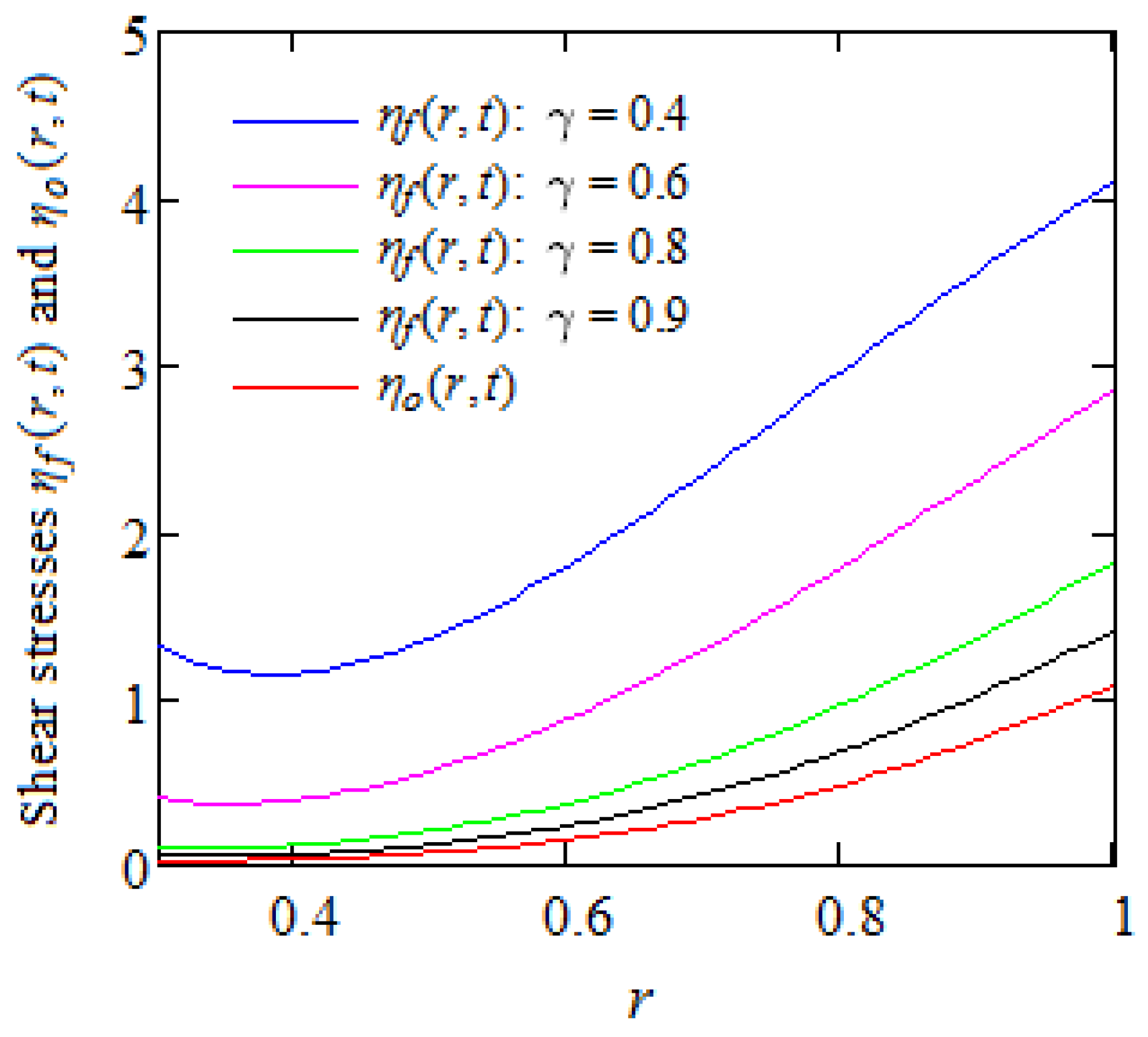
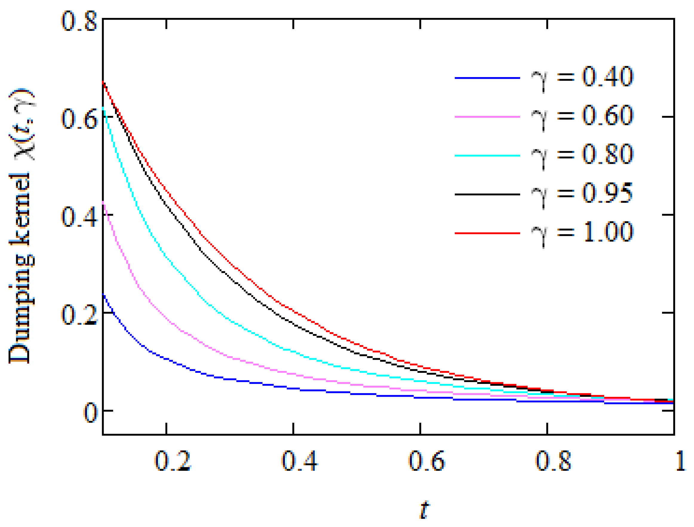
At small values of time t, the kernel $\chi (t,\gamma )$ increases with the fractional parameter. It follows that for small values of the fractional parameter, a weaker damping of the velocity gradient is achieved, and the shear stress values are therefore higher (see Figure 8).

–

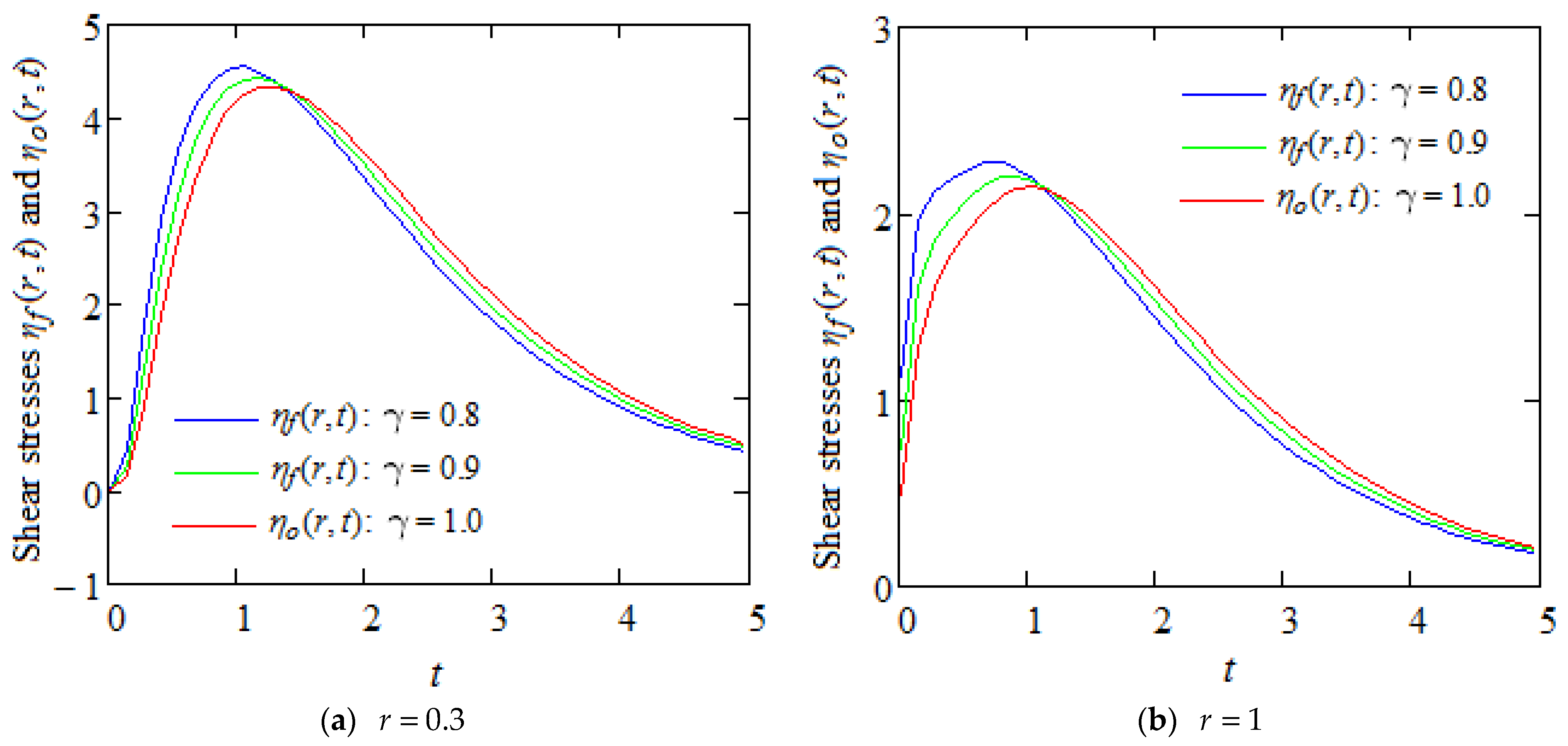
For large values of time t, the values of the two nuclei are almost identical; therefore, the difference between the fractional model and the ordinary model fades. It should be noted that there are significant differences between the two models only for small values of time t. Moreover, this property can also be seen in the graphs in Figure 9.

6. Conclusions

In this study, the MHD motion of ordinary and fractional ECIOBFs through a porous medium between two infinite coaxial circular cylinders is completely solved when the outer cylinder moves along its symmetry axis. Closed-form expressions were established for the dimensionless velocity field corresponding to both fluids, and the results were validated in a case study using graphical proof. All the solutions that were provided are new to the literature. Finally, some graphical representations were included in order to bring to light the characteristics of the fluids’ behaviors and to determine the time needed to reach a steady state, which is very important in practice.

We also mentioned the fact that the Oldroyd-B fluid flows studied in this paper are important because of their multiple potential theoretical and practical applications. Flows in porous channels are of considerable interest because they occur in many engineering and biomedical applications, such as the design of filters and porous pipes, gaseous diffusion, drilling mud, blood flow through capillaries, the dialysis of blood in an artificial kidney, etc. Additionally, magnetohydrodynamic motion is significant in the control of flows in metallurgical processes and several engineering applications, including nuclear reactors, geothermal energy extraction, and MHD generators.

The main outcomes of this study are as follows:

(1)

Exact general expressions were established for the dimensionless velocity fields of the isothermal MHD axial flows of ordinary and fractional ECIOBFs through porous annular channels.

(2)

These expressions can generate exact solutions for any flow of these kinds of fluids. To illustrate the concept, two particular cases were considered and investigated, and the validation of their results was given in Figure 2 and Figure 3.

(3)

It was proved for the first time that the flow of fractional ECIOBFs, due to the outer cylinder moving along its symmetry axis with a constant velocity V, becomes steady over time.

(4)

The steady components $w_{fs}(r)$ and $w_{os}(r)$ of the starting velocities $w_f(r,t)$ and $w_o(r,t)$ of ordinary and fractional ECIOBF flows are identical.

(5)

It was graphically proven that a steady state is reached earlier in fractional ECIOBFs compared with ordinary fluids.

(6)

This steady state is reached faster in the presence of a magnetic field and slower in the presence of a porous medium.

Finally, the present results can be extended to similar flows in Burgers fluids or to the MHD motion of these fluids when shear stress is added to the boundary as a governing equation for non-trivial shear stress can be obtained.

References

- Oldroyd, J.G. On the formulation of rheological equations of state. Proc. R. Soc. London Ser. A 1950, 200, 523–541. [Google Scholar] [CrossRef]
- Waters, N.D.; King, M.J. The unsteady flow of an elastico-viscous liquid in a straight pipe of circular cross section. J. Phys. D Appl. Phys. 1971, 4, 204–211. [Google Scholar] [CrossRef]
- Rajagopal, K.R.; Bhatnagar, R.K. Exact solutions for some simple flows of an Oldroyd-B fluid. Acta Mech. 1995, 113, 233–239. [Google Scholar] [CrossRef]
- Wood, W.P. Transient viscoelastic helical flow in pipes of circular and annular cross-section. J. Non-Newton. Fluid Mech. 2001, 100, 115–126. [Google Scholar] [CrossRef]
- Fetecau, C. Analytical solutions for non-Newtonian fluid flows in pipe-like domains. Int. J. Non-Linear Mech. 2004, 39, 225–231. [Google Scholar] [CrossRef]
- Fetecau, C.; Fetecau, C.; Vieru, D. On some helical flows of Oldroyd-B fluids. Acta Mech. 2007, 189, 53–63. [Google Scholar] [CrossRef]
- McGinty, S.; McKee, S.; McDermott, R. Analytic solutions of Newtonian and non-Newtonian pipe flows subject to a general time-dependent pressure gradient. J. Non-Newton. Fluid Mech. 2009, 162, 54–77. [Google Scholar] [CrossRef]
- Imran, M.; Tahir, M.; Imran, M.A.; Awan, A.U. Taylor-Couette flow of an Oldroyd-B fluid in an annulus subject to a time-dependent rotation. Am. J. Appl. Math. 2015, 3, 25–31. [Google Scholar] [CrossRef]
- Ullah, S.; Tanveer, M.; Bajwa, S. Study of velocity and shear stress for unsteady flow of incompressible Oldroyd-B fluid between two concentric rotating circular cylinders. Hacet. J. Math. Stat. 2019, 48, 372–383. [Google Scholar] [CrossRef]
- Tong, D.; Wang, R.; Yang, H. Exact solutions for the flow of non-Newtonian fluid with fractional derivative in an annular pipe. Sci. Chin. Ser. G 2005, 48, 485–495. [Google Scholar] [CrossRef]
- Tong, D.; Zhang, X.; Zhang, X. Unsteady helical flows of a generalized Oldroyd-B fluid. J. Non-Newton. Fluid Mech. 2009, 156, 75–83. [Google Scholar] [CrossRef]
- Qi, H.; Jin, H. Unsteady helical flow of a generalized Oldroyd-B fluid with fractional derivative. Nonlinear Anal. Real World Appl. 2009, 10, 2700–2708. [Google Scholar] [CrossRef]
- Kamran, M.; Imran, M.; Athar, M.; Imran, M.A. On the unsteady rotational flow of fractional Oldroyd-B fluid in cylindrical domains. Meccanica 2012, 47, 573–584. [Google Scholar] [CrossRef]
- Mathur, V.; Khandelwal, K. Exact solution for the flow of Oldroyd-B fluid between coaxial cylinders. Int. J. Eng. Res. Technol. (IJERT) 2014, 3, 949–954. [Google Scholar]
- Riaz, M.B.; Imran, M.A.; Shabbir, K. Analytic solutions of Oldroyd-B fluid with fractional derivatives in a circular duct that applies a constant couple. Alex. Eng. J. 2016, 55, 3267–3275. [Google Scholar] [CrossRef]
- Ullah, S.; Khan, N.A.; Liagat, K. Some exact solutions for the rotational flow of Oldroyd-B fluid between two circular cylinders. Adv. Mech. Eng. 2017, 9, 1–15. [Google Scholar] [CrossRef]
- Sadiq, N.; Imran, M.; Safdar, R.; Tahir, M.; Javaid, M.; Younas, M. Exact solution for some rotational motions of fractional Oldroyd-B fluids between circular cylinders. Punjab Univ. J. Math. 2018, 50, 39–59. [Google Scholar]
- Tahir, M.; Naeem, M.N.; Javaid, M.; Younas, M.; Imran, M.; Sadiq, N.; Safdar, R. Unsteady flow of fractional Oldroyd-B fluids though rotating annulus. Open Phys. 2018, 16, 93–200. [Google Scholar] [CrossRef]
- Song, D.Y.; Jiang, T.Q. Study on the constitutive equation with fractional derivative for the viscoelastic fluids-Modified Jeffreys model and its application. Rheol. Acta 1998, 27, 512–517. [Google Scholar] [CrossRef]
- Makris, N. Theoretical and Experimental Investigation of Viscous Dampers in Applications of Seismic and Vibration Isolation. Ph.D. Thesis, State University of New York at Buffalo, Buffalo, NY, USA, 1991. [Google Scholar]
- Bagley, R.L.; Torvik, P.J. A theoretical basis for the applications of fractional calculus to viscoelasticity. J. Rheol. 1983, 27, 201–210. [Google Scholar] [CrossRef]
- Friedrich, C. Relaxation and retardation functions of a Maxwell model with fractional derivatives. Rheol. Acta. 1991, 30, 151–158. [Google Scholar] [CrossRef]
- Heibig, A.; Palade, L.I. On the rest state stability of an objective fractional derivative viscoelastic fluid model. J. Math. Phys. 2008, 49, 043101–043122. [Google Scholar] [CrossRef]
- Mainardi, F. An historical perspective of fractional calculus in linear viscoelasticity. Fract. Calc. Appl. Anal. 2012, 15, 712–717. [Google Scholar] [CrossRef]
- Hristov, J. Constitutive Fractional Modeling. In Mathematical Modelling: Theory and Applications, Contemporary Mathematics; Hemen, D., Ed.; American Mathematical Society: Providence, RI, USA, 2023; Volume 786, pp. 37–140. [Google Scholar] [CrossRef]
- Tan, W.C.; Masuoka, T. Stokes’ first problem for an Oldroyd-B fluid in a porous half space. Phys. Fluids 2005, 17, 023101. [Google Scholar] [CrossRef]
- Hussain, M.; Hayat, T.; Fetecau, C.; Asghar, S. On accelerated flows of an Oldroyd-B fluid in a porous medium. Nonlinear Anal. Real World Appl. 2008, 9, 1394–1408. [Google Scholar] [CrossRef]
- Khan, I.; Imran, M.; Fakhari, K. New exact solutions for an Oldroyd-B fluid in a porous medium. Int. J. Math. Math. Sci. 2011, 2011, 408132. [Google Scholar] [CrossRef]
- Hayat, T.; Shehzad, S.A.; Mustafa, M.; Hendi, A. MHD flow of an Oldroyd-B fluid through a porous channel. Int. J. Chem. React. Eng. 2012, 10, A8. [Google Scholar] [CrossRef]
- Khan, M.; Ijaz, A. Starting solutions for an MHD Oldroyd-B fluid through porous space. J. Porous Media. 2014, 17, 797–809. [Google Scholar] [CrossRef]
- Riaz, M.B.; Awrejcewicz, J.; Rehman, A.U. Functional effects of permeability on Oldroyd-B fluid under magnetization: A comparison of slipping and non-slipping solutions. Appl. Sci. 2021, 11, 11477. [Google Scholar] [CrossRef]
- Hayat, T.; Hutter, K.; Asghar, S.; Siddiqui, A.M. MHD flows of an Oldroyd-B fluid. Math. Comput. Model. 2002, 36, 987–995. [Google Scholar] [CrossRef]
- Hayat, T.; Hussain, M.; Khan, M. Hall effect on flows of an Oldroyd-B fluid through porous medium for cylindrical geometries. Comput. Math. Appl. 2006, 52, 269–282. [Google Scholar] [CrossRef]
- Hamza, S.E.E. MHD flow of an Oldroyd-B fluid through porous medium in a circular channel under the effect of time dependent pressure gradient. Am. J. Fluid Dyn. 2017, 7, 1–11. [Google Scholar] [CrossRef]
- Fetecau, C.; Mirza, I.A.; Vieru, D. Hydrodynamic permeability in axisymmetric flows of viscous fluids through an annular domains with porous layer. Symmetry 2023, 15, 585. [Google Scholar] [CrossRef]
- Cao, W.; Kaleem, M.M.; Usman, M.; Asjad, M.I.; Almusawa, M.Y.; Eldin, S.M. A study of fractional Oldroyd-B fluid between two coaxial cylinders containing gold nanoparticles. Case Stud. Therm. Eng. 2023, 45, 102949. [Google Scholar] [CrossRef]
- Fetecau, C.; Vieru, D. Investigating Magnetohydrodynamic Motions of Oldroyd-B Fluids through a Circular Cylinder Filled with Porous Medium. Processes 2024, 12, 1354. [Google Scholar] [CrossRef]
- Ghazi, G.; Waleed, A. Impacts of porous medium on unsteady helical flows of generalized Oldroyd-B fluid with two infinite coaxial circular cylinders. Iraqi J. Sci. 2021, 62, 1686–1694. [Google Scholar] [CrossRef]
- Sneddon, I.N. Fourier Transforms; Mcgraw-Hill Book Company, Inc.: New York, NY, USA; Toronto, ON, Canada; London, UK, 1951. [Google Scholar]
Disclaimer/Publisher’s Note: The statements, opinions and data contained in all publications are solely those of the individual author(s) and contributor(s) and not of MDPI and/or the editor(s). MDPI and/or the editor(s) disclaim responsibility for any injury to people or property resulting from any ideas, methods, instructions or products referred to in the content. |
© 2024 by the authors. Licensee MDPI, Basel, Switzerland. This article is an open access article distributed under the terms and conditions of the Creative Commons Attribution (CC BY) license (https://creativecommons.org/licenses/by/4.0/).
Share and Cite
Fetecau, C.; Vieru, D.; Eva, L.; Forna, N.C. Memory Effects in the Magnetohydrodynamic Axial Symmetric Flows of Oldroyd-B Fluids in a Porous Annular Channel. Symmetry 2024, 16, 1108. https://doi.org/10.3390/sym16091108
Fetecau C, Vieru D, Eva L, Forna NC. Memory Effects in the Magnetohydrodynamic Axial Symmetric Flows of Oldroyd-B Fluids in a Porous Annular Channel. Symmetry. 2024; 16(9):1108. https://doi.org/10.3390/sym16091108
Chicago/Turabian StyleFetecau, Constantin, Dumitru Vieru, Lucian Eva, and Norina Consuela Forna. 2024. "Memory Effects in the Magnetohydrodynamic Axial Symmetric Flows of Oldroyd-B Fluids in a Porous Annular Channel" Symmetry 16, no. 9: 1108. https://doi.org/10.3390/sym16091108