Abstract
In this paper, the quadratic p-median optimization problem is discussed, where the goal is to connect users to a selected group of facilities (emergency services, telecommunications servers, healthcare facilities) at the lowest possible cost. The problem is aimed at minimizing the cost of connecting these selected facilities. The costs are symmetric, meaning connecting two different points is the same in both directions. This problem extends the traditional p-median problem, a combinatorial problem used in various fields like facility location, network design, transportation, supply chain networks, emergency services, healthcare, and education planning. Surprisingly, the quadratic version has not been thoroughly considered in the literature. The paper highlights the formulation of two mixed-integer quadratic programming models to find optimal solutions to this problem. One model is a classic formulation, and the other is based on set cover theory. Linear versions and Bender’s decomposition formulations for each model are also derived. A Bender’s decomposition is solved using an algorithm that adds constraints during each iteration to improve the solution. Lazy constraints in the Gurobi solver’s branch and cut algorithm are dynamically added whenever a mixed-integer programming solution is found. Additionally, an efficient local search meta-heuristic is proposed that usually finds optimal solutions for tested instances. Challenging instances with up to 60 facilities and 2000 users are successfully solved. Our results show that Bender’s models with lazy constraints are the most effective for Euclidean and random test cases, achieving optimal solutions in less CPU time. The meta-heuristic also finds near-optimal solutions rapidly for these cases.
1. Introduction
The quadratic p-median optimization problem goes like this: imagine there are a bunch of places where things can be located, called facility nodes, and a group of people who need those things, called users or customers. The idea is to pick the best group of facility nodes, denoted by , which is a subset of all the facility nodes , with a certain cardinality p. This chosen group should be the most cost-effective for connecting every user, ensuring each one is connected to a unique facility node in . Additionally, the cost of connecting every pair of facilities in is minimized. Notice that the cost of connecting users to facilities and connecting facilities themselves can be measured by the Euclidean distances or simply by considering randomly generated costs. The first cost is more intuitive since the larger the distances, the higher the costs for users and facilities. On the other side, random costs may appear in different situations when considering traffic jams, waiting times to arrive at a determined facility, and the demand of each facility to attend to a particular user, for instance. Also, notice that the cost of connecting facilities is not usually incorporated in the classic p-median problem [1,2,3]. Furthermore, when arranging how things are connected in a network on a diagram, the cost of connecting two places can be figured out by looking at the shortest distance between them [4]. Also, notice that all these costs are symmetric for the problem. Including these costs is important in many situations. For instance, during a pandemic like COVID-19, moving patients between hospitals incurs costs. Similarly, in a wireless network, placing facilities closer together allows for faster data transmission and lower power consumption. More application domains can include telecommunications to place cell towers or base stations to ensure network coverage and minimize signal interference, emergency service planning while identifying optimal locations for hospitals, fire stations, or police stations to reduce response times, and public services to locate schools, libraries, or community centers to serve the population effectively and equitably [5,6,7]. For more applications, the reader is referred to the works by [8,9,10,11]. These works relate to healthcare facility planning, e-commerce and distribution centers, disaster response and humanitarian logistics, and smart city planning.
To motivate the study of the quadratic p-median problem, it is worth highlighting its real-world applications and the challenges it addresses in practical scenarios. For example, the quadratic p-median problem is crucial in optimizing the location of facilities (like hospitals, schools, warehouses) to serve a population. Unlike the classical p-median problem, which minimizes the sum of distances between demand points and their nearest facility, the quadratic version also considers the interaction between facilities. In urban planning, it is not just about where to place facilities, but also how these facilities interact with each other. For example, locating hospitals too close might cause an overlap in their service areas, leading to inefficiencies. The quadratic p-median problem models these interactions, helping planners make decisions that minimize overall costs and maximize service efficiency. Similarly, in logistics, the placement of distribution centers or warehouses affects not only transportation costs but also operational efficiencies across the network. The quadratic p-median problem can model these complex relationships. As supply chains become more interconnected, the interaction between different nodes (warehouses, factories, etc.) becomes critical. Solving the quadratic p-median problem allows businesses to optimize the entire network, considering both direct and indirect costs, leading to more resilient and cost-effective supply chains. In telecommunications network design, such as cell towers or data centers, the quadratic p-median problem helps optimize the placement to ensure coverage while minimizing interference between nodes. It is not enough to just minimize the distance to users; the interaction between network nodes (like signal interference) is critical. The quadratic p-median problem incorporates these factors, leading to better network performance and user experience. Also, in healthcare, the placement of medical facilities like clinics or diagnostic centers needs to consider not just accessibility but also the interaction between facilities, such as patient referrals or resource sharing. Healthcare systems benefit from a holistic view where interactions between facilities (like referral patterns or shared resources) are considered. The quadratic p-median problem helps optimize facility placement to improve patient outcomes and system efficiency. In a similar contribution, the quadratic version of the p-median problem can be achieved in retail chains for deciding where to open new stores, which involves considering both customer accessibility and competition between stores in the same chain. Ultimately, the contribution to environmental and sustainability studies is mentioned when designing conservation areas or resource distribution networks. It is important to consider not only the locations but also the interaction between sites, like migration patterns or resource sharing. The quadratic p-median problem supports sustainability goals by optimizing spatial arrangements that consider both direct impacts (like resource access) and indirect interactions (like migration corridors), leading to more effective conservation strategies.
In this paper, two mixed-integer quadratic programming models are proposed to obtain optimal solutions to the problem. A classic one and a set cover-based formulation [12] are proposed. For each one of them, their linear counterparts and Bender’s decomposition formulations are derived. In particular, the latter models are solved using the classic Bender’s algorithm, which consists of adding optimality cuts within each iteration of the classic Bender’s algorithm and also by adding lazy constraints within the branch and cut algorithm of the Gurobi solver [13]. The latter is performed as follows. Whenever a mixed-integer programming (MIP) solution is obtained during the execution of the Gurobi branch and cut solver, if that MIP solution violates the optimality or feasibility cut, then a cut is added as a new lazy constraint to the problem. As will be seen later, the derived Bender’s decomposition models do not contain feasibility cuts since for each integer entry of variables there is always a feasible solution that can be obtained. Finally, an efficient local search method is introduced that usually finds the best solutions for each tested problem. Difficult problems with up to 60 facilities and 2000 users are solved. Extensive numerical tests to compare all the models are performed using Euclidean and randomly generated instances. To the best of our knowledge, our models are new to the field. Specifically, there are no Bender’s formulations for the quadratic p-median problem in existing research. This is also the first time these models are solved using a callback function with a top solver like Gurobi [13] to add lazy constraints and compare this with the classic Bender’s algorithm. Additionally, the proposed local search method is new for approximately solving this problem. To the best of our knowledge, in the literature, there are no approaches for the quadratic version of the p-median problem as proposed in our paper. Ultimately, it is mentioned that this paper is an extensive version of our previous work published in [14].
This paper is organized as follows: Section 2 reviews related work on the quadratic p-median problem and similar facility location problems. Section 3 explains a feasible solution to the problem and discusses some application domains for the solution presented. Whereas in Section 4, our proposed mathematical formulations are presented and explained. Section 5 details our algorithmic procedures. In Section 6, extensive numerical experiments are presented and compared with the proposed models, and algorithms. Finally, Section 7 summarizes our main conclusions and discusses potential directions for future research.
2. Related Work
In this section, some of the works that are closer to our paper are summarized. This paper is an extended version of our previous work published in [14]. In that earlier work, the problem of minimizing both the total connectivity cost for users to facility nodes and the cost of connecting the facilities themselves was addressed by solving hard instances with up to 60 facility nodes and 350 users using the Gurobi solver [13]. The numerical results showed that the linear set-covering formulation could solve all tested instances optimally with significantly less computational cost compared to other proposed models in [14].
In this extended paper, where the quadratic p-median optimization problem corresponds to an extended version of the classic p-median problem, a type of combinatorial optimization problem is explored in more detail. Thus, the models in [14] are considered in this paper where the first one corresponds to a classic formulation and the other one to a set covering based-formulation. However, now their linear versions and their Benders’ decomposition variants of the models are further derived. Consequently, Bender’s models with the classic Bender’s algorithm [15], and also by adding lazy constraints within the branch and cut algorithm of the Gurobi solver, are solved. Finally, a fast meta-heuristic local search method that allows for finding near-optimal solutions to the problem is proposed. All the new models and proposed solving methods are tested on difficult instances with up to 60 locations and 2000 users successfully. As a final contribution of this large version of the paper in [14], substantial numerical results indicate that Bender’s models with lazy constraints are the most effective for the Euclidean and randomly tested instances in terms of finding the optimal solutions in significantly less CPU times. Ultimately, the meta-heuristic also finds near-optimal solutions in short CPU times for both the Euclidean and randomly generated instances.
In the current literature, a classic study by [16] introduced a new integer quadratic model for a general hub-location problem. The study explores different methods, including two simpler ones, to choose locations for two, three, or four hubs to connect groups of 10, 15, 20, and 25 cities. Interestingly, the quadratic version of the classic p-median problem has not been deeply explored yet.
Other relevant works include studies on wireless networks and urban planning, where similar methods can be applied. For example, [17] discusses placing multiple sink nodes in a wireless sensor network using a method related to the p-median problem. This approach can reduce energy consumption, improve network performance, and extend its lifespan. In another study, ref. [18] uses big data for urban planning to better model cities and use resources efficiently. They propose a robust computer-based approach using random sampling and spatial voting to solve large p-median problems, demonstrating that their method finds good solutions quickly and performs well even when the problem size changes. In [19], the authors revisit a Cornuéjols-Nemhauser-Wolsey formulation for the p-median problem. Even though this formulation has the fewest variables, it is rarely used or mentioned in research. The authors combine a selection problem with extra rules to correctly define the costs. They also prove that the simplified version of this formulation is the same as the simplified version of the classic formulation. By examining some extra rules, they discuss ways to find solutions for large problems. These methods involve simplifying the problem by removing some of the extra rules, which can help solve large problems more easily. Finally, they present tests showing that this updated formulation can be effectively used to solve p-median problems. Similarly, in [20], the study focuses on the Hamiltonian p-median problem, where from a given graph with weighted edges it is required to find p separate cycles that cover all the vertices of the graph to minimize the total weight. The authors introduce two new types of constraints for solving this problem using edge variables. Finally, they propose branch-and-cut algorithms based on these constraints and additional ones that remove less optimal solutions. Tests on standard problem sets show that their algorithms perform similarly to existing exact methods and can solve new problems with up to 400 vertices.
Because of the lack of references considering the quadratic version of the p-median problem, the reader is referred to the literature concerning facility location and classic p-median problems where our proposed models in this paper can certainly be applied. See, for instance, the works [21,22,23].
3. A Feasible Solution to the Quadratic p-Median Problem
In this section, a feasible solution to the quadratic p-median problem is presented. An optimal, i.e., the best feasible, solution to the quadratic optimization problem is depicted in Figure 1.
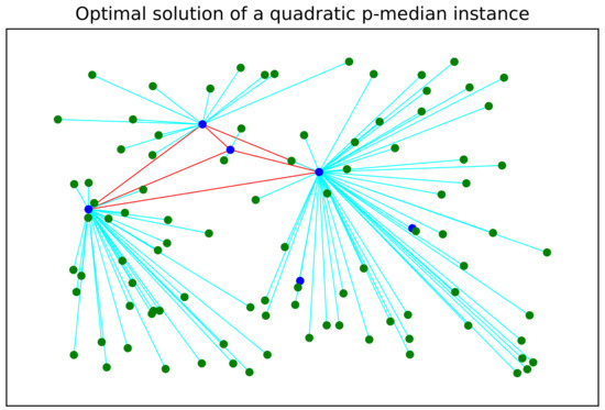
Figure 1.
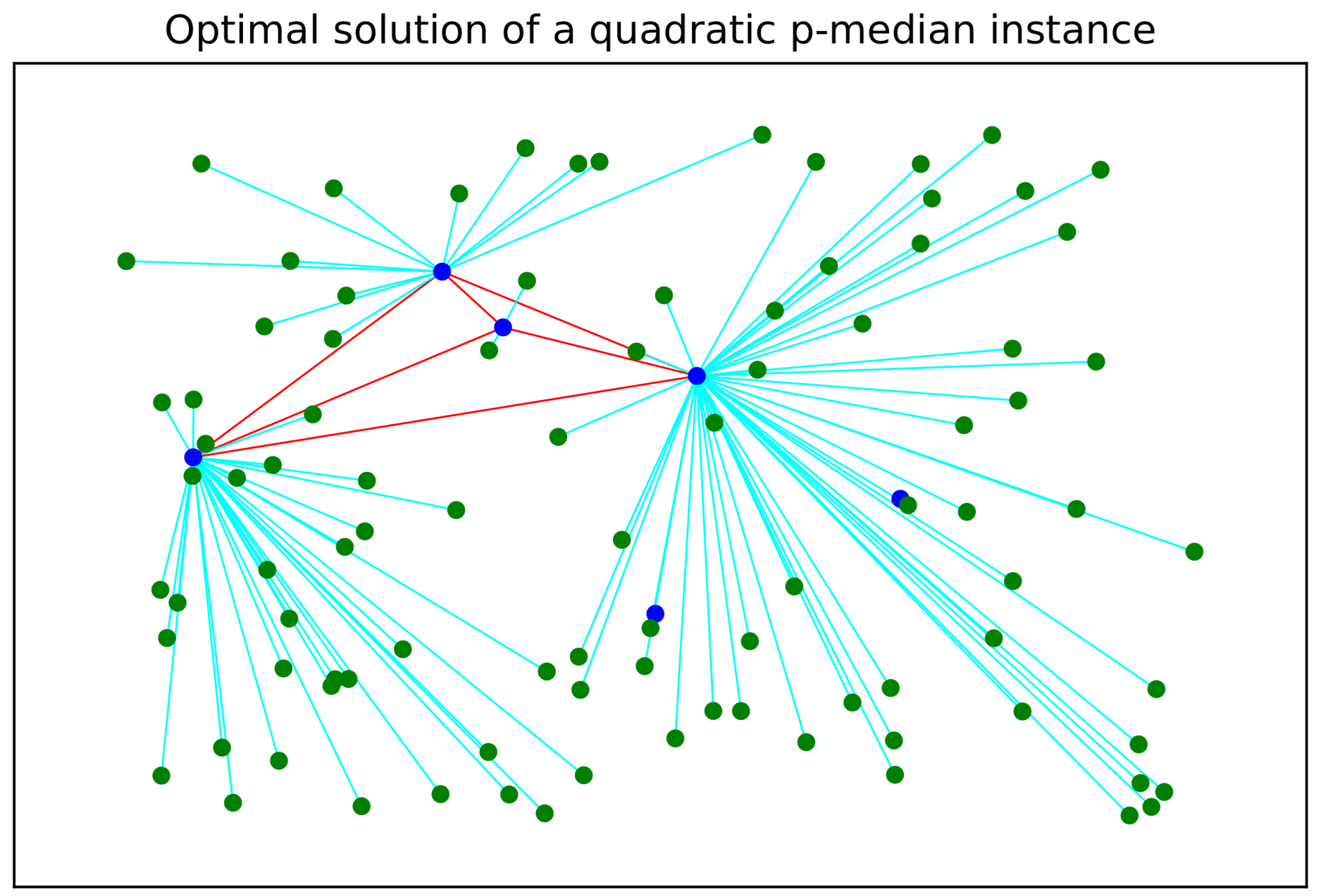
Optimal (best feasible) solution obtained for a Euclidean randomly generated graph composed of 6 candidate locations of facilities and 100 users. Users are colored green whereas facilities are colored blue. The connection links between facilities are colored red and each connection link of each user to its nearest facility is colored cyan.
From the optimal solution, it is easy to see that only four blue facilities are fully connected, i.e., forming a clique sub-graph. Similarly, each user is connected to its nearest blue active facility. As can be seen from Figure 1, only two facilities are discarded from the optimal solution.
The graph in Figure 1 represents an optimal solution for a quadratic p-median problem. In this kind of problem, you choose certain locations (medians) to minimize the total distance between demand points and these medians, while also considering the relationship between pairs of medians. Some applications for a network like this can be enumerated as follows:
- Telecommunication Networks: choosing the best places to put antennas or servers to ensure good coverage and fast communication.
- Transportation Routes: deciding the best locations for distribution centers to make sure products are delivered quickly and cheaply.
- Supply Chains: finding the best spots for factories or warehouses to efficiently meet the demand of stores or customers.
- Urban Planning: placing public services like hospitals or fire stations in spots where they can respond quickly to emergencies.
- Social Networks: identifying key people or groups in a social network to spread information or influence effectively.
- Electric Power Grids: choosing the best locations for substations to ensure efficient energy distribution with minimal loss.
- Logistics: determining the best locations for delivery centers to reduce transportation costs and improve delivery times.
Each of these applications can be modeled and solved using various optimization techniques depending on the specific requirements and complexity of the problem. Our quadratic version of the p-median problem constitutes a good reference for more specific modeling approaches.
4. Mathematical Formulations
In this section, the mixed-integer quadratic and linear models are presented, explained, and described. Finally, it is explained how Bender’s models from the MIP formulations are obtained.
To create the initial quadratic model, the following 0–1 variables are defined:
and
They define the input matrices for all and , and the symmetric matrix for all . Each element of these matrices represents the distances or costs between elements i and j. In particular, each element in matrix C represents the distance cost between users and facilities. Each matrix element in D corresponds to the distance cost between facilities. Therefore, the first model can be written as follows.
Model is an extension of the classic p-median problem [1,2,3]. The main difference is the second quadratic term in the goal Formula (1). In this formula, the first part shows the costs of connecting users to facilities, while the second part shows the costs of connecting facilities. The first set of constraints (2) ensures that each user , where , is connected to exactly one facility node . The constraint (3) selects p facilities out of n from the set . Then, constraints (4) state that each user should be linked to a facility node if j is part of the solution. Finally, the constraints (5) determine the limits for the decision variables.
Another way to create a linear version of is by using the standard linearization method [24]. This procedure consists of replacing each quadratic term in the objective with a new variable for all while adding three sets of linear constraints, thus leading to the following formulation.
Notice that the objective Function (6) is linear now. Whereas the constraints (7)–(9) indicate that if and for all where . Otherwise, .
To create another equivalent set-covering formulation [12], we proceed in the following manner. First, the additional input matrix for each and is defined where plus and additional artificial node placed at the beginning of . Next, this matrix is initialized as an empty matrix. Then, for each , the corresponding row vector of matrix is sorted in ascending order, for all . The resulting vector corresponds to the row of . Lastly, an extra zero column vector is added to the left of matrix . Similarly, the input symmetric matrix for all is defined. This matrix adds a zero column and a row vector to the left and at the top of D, respectively. Then, the following cumulative variables are defined.
As a result, it is also possible to write a new quadratic p-median formulation like this:
which can be linearized as
Note that the linear constraints (16)–(18) now apply in for all , where . Also, these constraints are similar to those in the first and second models, so their explanations are skipped. For more details on the radial constraints (13), you can check [12,14]. Now, let us move on to Bender’s formulations.
Bender’s Formulations
To derive Bender’s formulations from and , one can proceed as follows [15]. First, to write the sub-problem from , i.e., the resulting model from , all the expressions from the objective function and constraints that contain continuous variables are needed. For a deeper comprehension of Bender’s decomposition method, the reader is referred to the work by [15].
Proposition 1.
The following linear Bender’s decomposition problem is equivalent to
where denotes the set of optimality cuts that are added during the resolution of .
Proof.
From , the following linear programming sub-problem is obtained, denoted hereafter by
Next, the dual formulation of is derived. For this purpose, the Lagrangian function of is defined as
Consequently, its dual linear formulation can be written as [25]
Finally, the following master problem is obtained
Notice that this model cannot be solved with the Gurobi solver [13] due to the quadratic constraints (32). Consequently, its linear version by introducing the variables [24] leading to is solved. □
Observation 1.
For any input variable y satisfying constraint (3) in , there is always a feasible solution for the quadratic p-median problem. Consequently, only optimality cuts are required and generated for solving model .
Notice that Observation 1 is also valid for solving , i.e., only optimality cuts are generated for .
To obtain an alternative Bender’s formulation from , we proceed similarly to .
Proposition 2.
The following linear Bender’s decomposition problem is equivalent to
where the set denotes analogously to the set of optimality cuts that are added during the resolution of .
Proof.
First, the linear programming sub-problem of is written as follows
Thus, the Lagrangian function reads
Its dual linear program can be written as
Finally, the master problem can be written as
Analogously, this model cannot be solved due to the quadratic constraints (43). Consequently, its linear version can be solved by introducing the variables , which leads us to model . □
To finalize this section, it is important to note that all these proposed models are with exponential time complexity and consequently difficult to solve in a reasonable amount of CPU time [26].
5. Algorithmic Approaches
In this section, first, the classic Bender’s algorithmic approach is presented, which allows us to optimally solve each of the master problems presented so far. Then, we discuss and explain the algorithm that adds optimality cuts during the execution of the branch and cut solver of Gurobi [13]. Finally, an efficient local search meta-heuristic is presented that allows for obtaining, in most cases, the optimal solutions for each tested instance.
5.1. Classic Bender’s Decomposition Algorithm
The classic Bender’s decomposition algorithm is used to solve optimization problems with separation structures. A simple explanation of how it works is given by describing the following steps. First, it starts with an initial integer feasible solution for the overall problem. Then, the dual sub-problem is solved. If the solution of the dual is bounded, then it allows us to obtain a new integer feasible solution that can be used to generate a new optimality cut to add to the master problem. On the opposite, if the solution of the dual is unbounded, then a feasibility cut must be added to the master problem. The process is repeated while a convergence criterion is not met, such as finding an optimal solution or no longer improving the current solution [15]. Bender’s decomposition algorithm helps solve optimization problems with separation structures since it breaks down the big problem into smaller sub-problems. By handling these smaller sub-problems independently, it can speed up the solving process for large-scale instances of the problem.
However, its effectiveness depends on how well the constraints for the sub-problems are generated and how efficiently the Benders sub-problems are solved. Since observation 1 related to the quadratic p-median problem guarantees that no feasibility cuts are generated for any input vector y, in Algorithm 1, the classic Bender’s algorithm adapted to our master problem is depicted. For illustration purposes, it is assumed that is being solved, although it can be used to solve . In Algorithm 1, the parameters , , and denote initial values of the upper bound, lower bound, and the tolerance for finding an optimal solution. Finally, the parameter denotes the maximum CPU time given to run the algorithm. The rest of the algorithm is self-explained.
| Algorithm 1: Classic Bender’s decomposition algorithm for solving the master problem . |
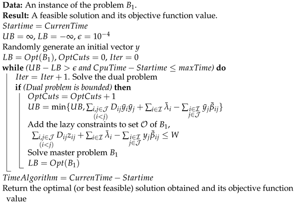 |
Notice that Algorithm 1 should provide the optimal solution to the problem without using the parameter. Thus, in case a solution reported is obtained in less than the pre-defined CPU time allowed in parameter , it means the algorithm has obtained the optimal solution to the problem.
Also, notice that solving a mixed-integer programming problem is of the order of , where r denotes the number of variables in the problem. Consequently, Algorithm 1 is of the order of the exponential bound .
5.2. Bender’s Decomposition Algorithm Adding Lazy Constraints
To solve either model or , lazy constraints are generated and added in a cutting plane form. Whenever an MIP solution is obtained during the resolution of the branch and cut algorithm of the Gurobi solver [13], an optimality cut (32) or (43) may be violated, if so, the corresponding valid inequality is added to the respective model or . The pseudocode of the procedure is depicted in Algorithm 2 for solving for illustration purposes.
| Algorithm 2: Bender’s decomposition algorithm embedded as a cutting plane into the branch and cut of the Gurobi solver for solving the master problem . |
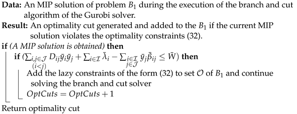 |
Algorithms 1 and 2 are both self-explained, and they are run in our numerical results section for a maximum CPU time arbitrarily set to at most one hour of CPU time. Consequently, in case a solution is obtained before one hour, it means that an optimal solution to the problem has been found. Otherwise, the solution corresponds to lower bounds in both cases since not all the constraints are added to the problem. Notice that deterministic constraints and lazy ones are not equivalent. The former ones are put in the model from the beginning. However, the lazy constraints are only added dynamically during the execution of the algorithm. Lazy constraints in Gurobi are a powerful feature used in Mixed-Integer Programming models. They are constraints that are not included in the initial model but are instead added during the solving process only when needed. This is useful in cases where the full set of constraints is too large to include initially, or where some constraints are only relevant to certain parts of the solution space.
Since Algorithm 2 is embedded into the branch and cut of the Gurobi solver, which is of the order of , where r denotes the number of variables in the problem, then Algorithm 2 is of the same exponential order . However, it is important to note that in this case the optimization problem is solved only once compared to the classic Bender’s algorithm which solves an exponential problem within each iteration.
5.3. A Local Search Meta-Heuristic Approach
In this subsection, a meta-heuristic local search for the quadratic p-median problem is proposed. The procedure is depicted in Algorithm 3 and works as follows. It requires as input an instance of the quadratic p-median problem and returns a feasible solution to the problem together with its objective function value. The algorithm first randomly generates an input permutation vector with the labeled index set corresponding to the facilities of the problem. Then, this permutation vector is split into two sub-lists. One is composed of p entries denoted by and another one with elements denoted by . Then, it enters into a while loop for a maximum number of iterations controlled by parameter . Before this, some parameters are also initialized, the , and the minimum global objective value as the worst initial value is equal to infinite since the optimization problem is being minimized.
| Algorithm 3: Proposed Local Search Meta-heuristic algorithm. |
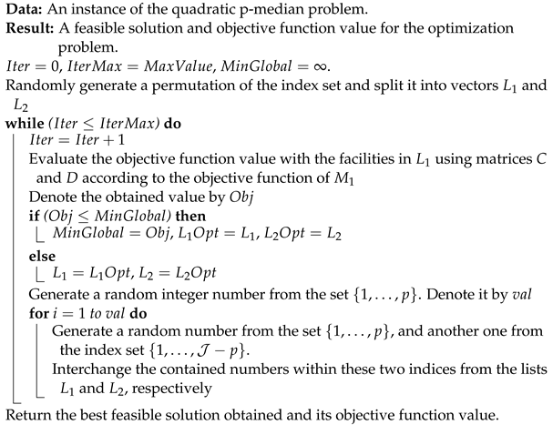 |
Inside the while loop, it computes the objective function value of model using matrices C and D for the input list . Let us denote this value by . If is less than the best objective value found so far, then we save the current solution and its objective value. Otherwise, we continue with the vectors and as the current best solution lists. Subsequently, a random integer value from the set is generated, and this number of interchanges between the elements of the lists and is applied, thus generating another possible solution in . The procedure continues iteratively performing the same steps. When the number of iterations is reached in the while loop, Algorithm 3 stops and returns the best solution found and its objective function value. Finally, the complexity order of Algorithm 3 is cubically bounded by the expression . This is because an evaluation of the objective function of is the most time-consuming step within the algorithm.
6. Results and Discussion
This section shows the numerical tests for all the proposed models and algorithms. A Python program with the Gurobi solver version 11.0.1 was developed for this purpose. The solver ran with its default settings. A maximum time limit of 1 h for each test was arbitrarily set. The tests were conducted on a computer with an Intel 64-bit core, 3 GHz processor, 8 GB of RAM, running Windows 10. 24 Euclidean and 24 random instances with dimensions of facilities, users, and nodes were generated in each network acting as candidate sites for the instances.
The input matrices and were created by calculating the distances between users and facilities and between facilities themselves. Matrix D is symmetric. The coordinates of each facility and user node for the Euclidean instances were drawn from the interval according to a uniform distribution function. While for the randomly generated instances, each entry in the cost matrices and for all and were drawn from the intervals and according to uniform distribution functions as well, respectively. The latter is based on the fact that connecting two facilities is commonly more expensive than connecting a user to a facility node in the network.
In Table 1, numerical results for the models , , and , using Euclidean instances are reported. Columns 1–4 show the instance number and the values of p, m, and n. Columns 5–8 show the best objective values for and found within 1 hour of CPU time, the number of branch and bound nodes, the CPU time in seconds required to obtain the best objective values, and the MipGaps from the Gurobi solver. The MipGap is calculated by subtracting the best lower bound from the best solution found and then dividing by the best solution. These values are given as percentages. If the Gurobi solver obtains an optimal solution, the MipGap equals zero and the CPU time is less than 1h. In columns 9–12, the same information for the models and are reported, respectively. Finally, notice that in Table 2, the same information as in Table 1 is presented but for random instances.

Table 1.
Results obtained with , , and , , respectively, for Euclidean instances.
Table 2.
Results obtained with , , and , , respectively, for random instances.
In Table 1, it is observed that all the instances can be solved optimally in less than 1h. Notice that all the Mipgaps equal zero for all the instances. In particular, the behavior of the quadratic models is slightly better than those of the linear ones as it can be verified by the CPU times required to obtain the optimal solutions. Moreover, a slightly better performance of is observed compared to in terms of CPU times as well.
On the other side, from Table 2, it is observed that for the random instances, the picture is completely different. First, it is noted that not all of the instances can be solved optimally, neither using the quadratic nor the linear models. It can be seen that many of the instances reach 3600 s with non-negative Mipgaps. Consequently, it is not possible to ensure that the best objective values reported are the optimal ones. In general, from Table 2, it is also difficult to discriminate which of the four models , , , or has a better performance. The random instances are significantly harder to solve than the Euclidean ones. Notice that random instances are also as important as the Euclidean ones since the input values of the matrices C and D can represent real-life costs instead of distances.
In Table 3 and Table 4, numerical results obtained with the models , by directly using Algorithm 2 are reported. Numerical results for and using the classic Algorithm 1 for the Euclidean and random instances are also presented, respectively. In particular, the legends of these tables are as follows. From columns 1–4, the instance number and the instance dimensions are presented. Recall that these instances are the same as those presented in Table 1 and Table 2, respectively. Next, in columns 5–8, the best objective function values, the number of branch and bound nodes, the CPU times, and the number of lazy constraints added during the execution of the branch and cut algorithm of the Gurobi solver using Algorithm 2 are reported. Next, columns 9–11 show the best solution obtained in at most one hour of CPU time, the CPU time in seconds, and the number of optimality cuts added to either or during the execution of Algorithm 1, respectively.
Table 3.
Results obtained with models , using Algorithms 2 and 1, respectively, for the Euclidean instances.
Table 4.
Results obtained with models , using Algorithms 2 and 1, respectively, for the random instances.
From Table 3, it can be seen that all the problems are solved optimally in less than 1 h of CPU time. The CPU times are all roughly the same. There is no noticeable difference between the two methods for the Euclidean instances. Lastly, it is noticed that there are fewer lazy constraints than optimality cuts. From Table 4, it can be seen that for the random instances, the problems are harder to solve optimally in at most 1 hour of CPU time. It is observed that a few instances could not be solved optimally in one hour. In summary, one can say that the best combination is using Algorithm 2 with model ; in this case, only one of the instances cannot be solved optimally. Regarding the CPU times, it is also observed that, in general, all of them are in the same order of magnitude for all the approaches. Lastly, the number of lazy constraints added is slightly larger than the optimality cuts. Notice, however, that solving Algorithm 2 either with models or is solved only once. Instead, the classic Bender’s approach requires solving several mixed integer programming master problems within each iteration. The latter leads us to conclude that using Algorithm 2 is preferable. Hereafter, solving model means solving model with Algorithm 2.
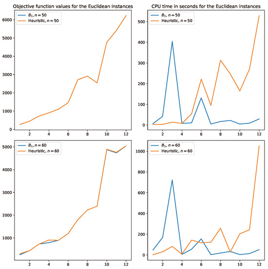
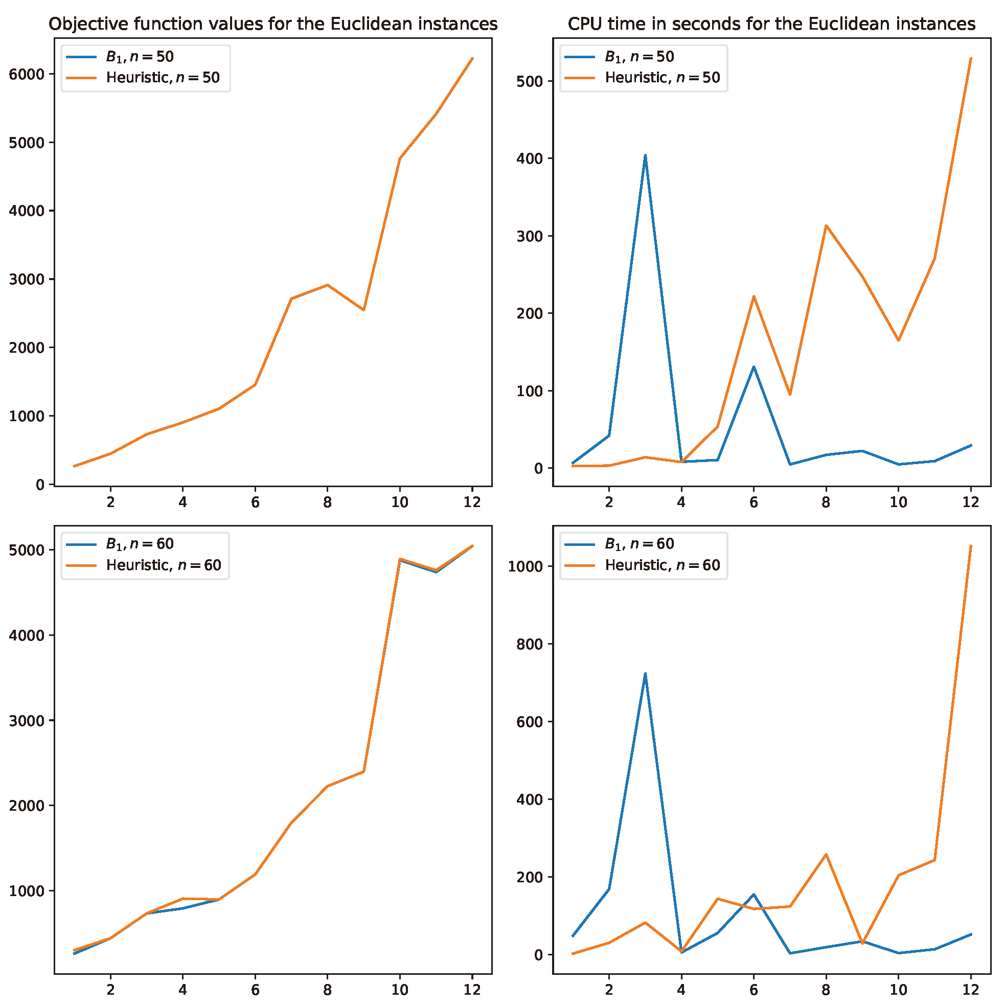
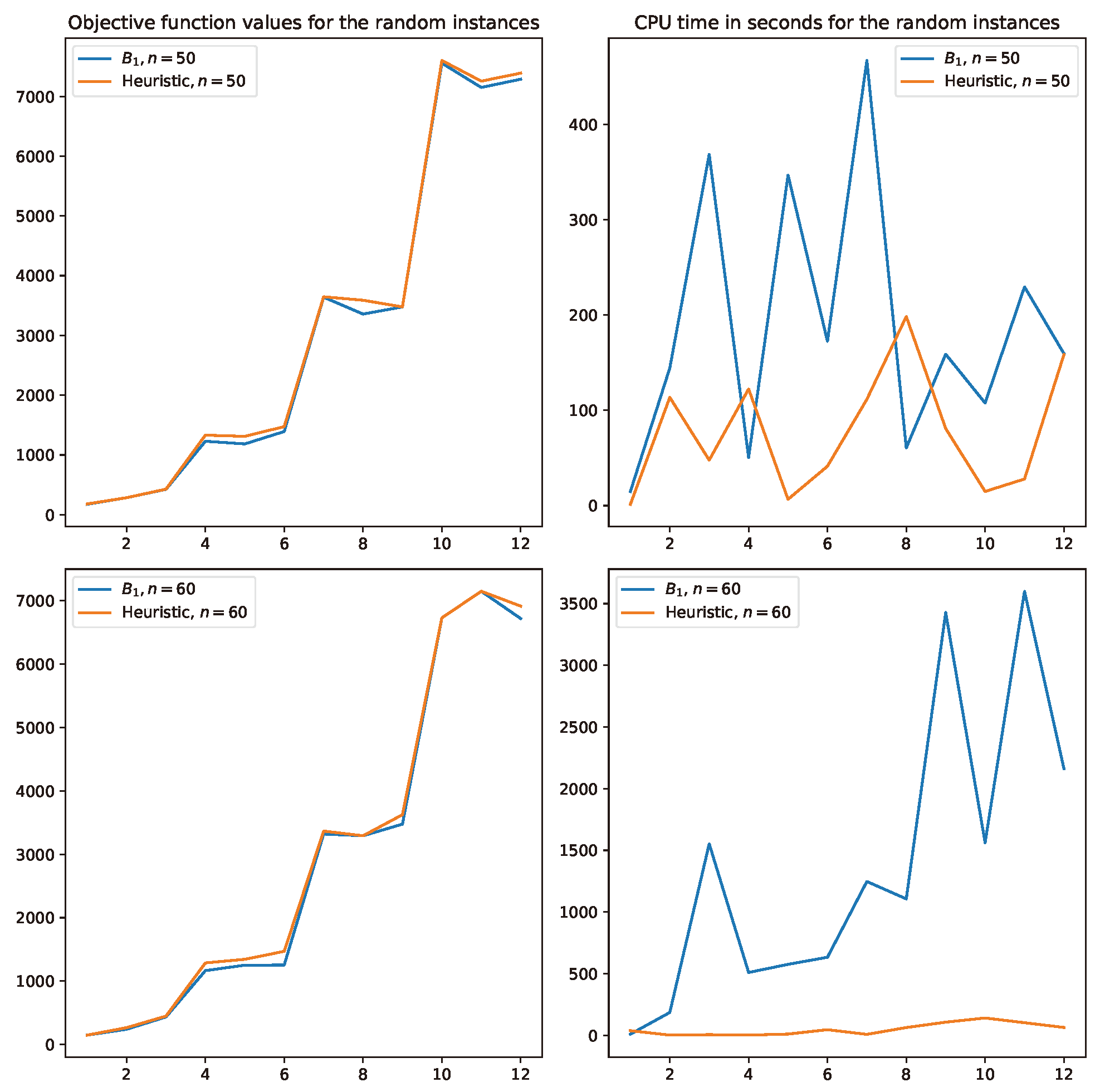
Concerning the proposed heuristic Algorithm 3, in Figure 2 and Figure 3, curves for the objective function values and CPU times obtained for the Euclidean and randomly generated instances of Table 1, Table 2, Table 3 and Table 4 are reported, respectively. From both figures, a similar trend is observed. First, Algorithm 3 is nearly optimal. Indeed, it is observed that many of the Euclidean instances obtain optimal solutions. In random instances, almost all objective values are nearly above the optimal solutions. Regarding the CPU times obtained, in Figure 2, it is observed that the heuristic takes a longer time than model requires to obtain the optimal solutions. On the other hand, in Figure 3, the opposite situation is observed, as one can see that for most of the instances, the meta-heuristic requires significantly less CPU time than solving each instance with model . Recall that the random instances are significantly harder to solve than the Euclidean ones. Consequently, Algorithm 3 is a clear contribution in this case.

Finally, in Figure 4, the optimal solutions for an input graph composed of nodes using a value of , and users are plotted. These graphs are obtained while varying the value of in the objective function of . Notice that for any value of , a clique sub-graph formed with blue facility nodes of cardinality is observed, and all users are connected to a unique blue node. Two blue nodes are isolated, which means that these two nodes are not part of the output solution of the problem.
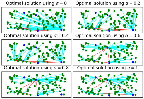
Figure 4.
Optimal solutions obtained for an input graph composed of candidate site facility nodes while using a value of , and users. In the graph, facility nodes are colored blue while users are colored green. The connections are colored cyan.
It is important to mention that since the input parameters are deterministic, the stability behavior of the models and algorithms is robust enough to obtain the same results, and only the meta-heuristic can vary with uncertainty. However, for all our tested instances, all the solving methods proved to be robust.
The next section presents a summary of the key findings of this paper, highlighting the most important points. Some thoughts on what these results mean and how they might influence future studies in this area are offered. Additionally, suggestions for possible directions of further research are mentioned while pointing out areas that could benefit from deeper exploration. Our goal is to provide a clear and concise wrap-up, along with ideas that could guide future work on this topic. Finally, the broader implications of our findings for both theory and practical applications are briefly discussed.
7. Conclusions
This paper addresses the quadratic p-median optimization problem, which focuses on minimizing the connection costs between users and a selected subset of facility nodes, as well as the connection costs among the facility nodes themselves. This problem can be seen as an extension of the classic p-median problem, which is widely known and applied in various fields of engineering. The classic p-median problem is relevant in areas such as facility location, network design for telecommunications, transportation systems, supply chain networks, emergency service planning, healthcare management, and educational resource planning, among others. The quadratic version of the problem extends the application to all these domains, considering not only the connection between users and facilities but also the interactions between the facilities themselves.
To address this complex problem, the paper proposes two mixed-integer quadratic programming models that are capable of finding optimal solutions. The first is a classic model, and the second is based on a set-covering formulation. For both models, their linear counterparts are also developed, and Bender’s decomposition formulations are derived to enhance the solution process. Specifically, these Bender’s models are solved using the traditional Bender’s algorithm, which involves adding optimality and feasibility cuts during each iteration. Additionally, lazy constraints are incorporated within the branch-and-cut algorithm of the Gurobi solver whenever a mixed-integer programming solution is obtained.
Moreover, the paper suggests a fast meta-heuristic method to explore the feasible solution space, which often finds the best solutions for the cases tested. The effectiveness of the proposed approaches is tested in challenging scenarios with up to 60 facility nodes and 2000 users. The results indicate that the classic Bender’s model with lazy constraints performs exceptionally well for Euclidean cases, quickly finding optimal solutions. However, for random cases, finding the best solutions proves to be much more difficult, with some instances remaining unsolved even after an hour of computation. Therefore, the study concludes that for random cases, the best approach is to use lazy constraints with the set-covering-based model, as this method consistently solves all instances faster. In addition, the rapid search method demonstrates its capability by finding nearly optimal solutions for random instances, offering a practical and efficient alternative for solving complex quadratic p-median problems.
In future research, new ways to model and solve this challenging quadratic combinatorial optimization problem will be explored. Additionally, new cutting-plane methods should be developed alongside these models to improve solution efficiency. The problem should also be adapted to fit more specific network applications, ensuring relevance to real-world scenarios. These future directions not only aim to refine existing methods but also seek to apply these sophisticated techniques to areas that are poised to shape the future, ensuring that this research remains at the forefront of technological advancement.
Author Contributions
Conceptualization, P.A., A.V. and A.D.F.; methodology, P.A., A.V. and A.D.F.; software, P.A. and A.V.; validation, P.A. and A.V.; formal analysis, P.A., A.V. and A.D.F.; investigation, P.A., A.V. and A.D.F.; resources, P.A. and A.D.F.; data curation, P.A., A.V. and A.D.F.; writing—original draft preparation, P.A., A.V. and A.D.F.; writing—review and editing, P.A. and A.V.; visualization, P.A., A.V. and A.D.F.; supervision, P.A.; project administration, P.A. and A.D.F.; funding acquisition, P.A. and A.D.F. All authors have read and agreed to the published version of the manuscript.
Funding
The authors acknowledge the financial support from Projects Dicyt 062313AS,ANID/FONDECYT Iniciación No. 11230129, and the Competition for Research Regular Projects, year 2021, code LPR21-02; Universidad Tecnológica Metropolitana.
Data Availability Statement
Dataset available on request from the authors: the raw data supporting the conclusions of this article will be made available by the authors on request.
Acknowledgments
The authors acknowledge the support of the Vicerrectoría de Investigación, Innovación y Creación (VRIIC) of the Universidad de Santiago de Chile.
Conflicts of Interest
The authors declare no conflicts of interest.
References
- Adasme, P. p-Median based formulations with backbone facility locations. Appl. Soft Comput. 2018, 67, 261–275. [Google Scholar] [CrossRef]
- Hakimi, S.L. Optimum location of switching centers and the absolute centers and medians of a graph. Oper. Res. 1964, 12, 450–459. [Google Scholar] [CrossRef]
- Mak, H.Y.; Shen, Z.J.M. Integrated Modeling for Location Analysis. Found. Trends Technol. Inf. Oper. Manag. 2016, 9, 1–152. [Google Scholar] [CrossRef]
- Cormen, T.H.; Leiserson, C.E.; Rivest, R.L.; Stein, C. Introduction to Algorithms; MIT Press and McGraw-Hill: Cumberland, RI, USA, 2009. [Google Scholar]
- Church, R.L.; Murray, A.T. Business Site Selection, Location Analysis, and GIS; John Wiley & Sons: Hoboken, NJ, USA, 2009. [Google Scholar] [CrossRef]
- Wang, W.; Wu, S.; Wang, S.; Zhen, L.; Qu, X. Emergency facility location problems in logistics: Status and perspectives. Transp. Res. Part Logist. Transp. Rev. 2021, 154, 102465. [Google Scholar] [CrossRef]
- Drezner, Z.; Hamacher, H.W. Facility Location: Applications and Theory; Springer Science & Business Media: Berlin/Heidelberg, Germany, 2002. [Google Scholar]
- Hoadley, E.D.; Jorgensen, B.; Masters, C.; Tuma, N.; Wulff, S. Strategic Facilities Planning: A Focus On Health Care. J. Serv. Sci. (JSS) 2010, 3. [Google Scholar] [CrossRef]
- Pajić, V.; Andrejić, M.; Jolović, M.; Kilibarda, M. Strategic Warehouse Location Selection in Business Logistics: A Novel Approach Using IMF SWARA–MARCOS—A Case Study of a Serbian Logistics Service Provider. Mathematics 2024, 12, 776. [Google Scholar] [CrossRef]
- Özdamar, L.; Ertem, M.A. Models, solutions and enabling technologies in humanitarian logistics. Eur. J. Oper. Res. 2015, 244, 55–65. [Google Scholar] [CrossRef]
- Hammad, A.W.; Akbarnezhad, A.; Haddad, A.; Vazquez, E.G. Sustainable Zoning, Land-Use Allocation and Facility Location Optimisation in Smart Cities. Energies 2019, 12, 1318. [Google Scholar] [CrossRef]
- García, S.; Labbé, M.; Marín, A. Solving Large p-Median Problems with a Radius Formulation. INFORMS J. Comput. 2011, 23, 546–556. [Google Scholar] [CrossRef]
- Achterberg, T. Gurobi Solver. Available online: https://www.gurobi.com/ (accessed on 25 June 2024).
- Sandoval, C.; Adasme, P.; Firoozabadi, A.D. Quadratic p-Median Formulations with Connectivity Costs between Facilities. In Mobile Web and Intelligent Information Systems; Bentahar, J., Awan, I., Younas, M., Grønli, T.M., Eds.; MobiWIS 2021. Lecture Notes in Computer Science; Springer: Cham, Switzerland, 2021; Volume 12814. [Google Scholar] [CrossRef]
- Rahmaniani, R.; Crainic, T.G.; Gendreau, M.; Rei, W. The Benders decomposition algorithm: A literature review. Eur. J. Oper. Res. 2017, 259, 801–817. [Google Scholar] [CrossRef]
- O’Kelly, M.E. A quadratic integer program for the location of interacting hub facilities. Eur. J. Oper. Res. 1987, 32, 393–404. [Google Scholar] [CrossRef]
- Haicheng, L. Research on Distribution of Sink Nodes in Wireless Sensor Network. In Proceedings of the 2010 Third International Symposium on Information Science and Engineering, Shanghai, China, 24–26 December 2010; pp. 122–124. [Google Scholar] [CrossRef]
- Wangshu, M.; Daoqin, T. On solving large p-median problems. Environ. Plan. Urban Anal. City Sci. 2020, 47, 981–996. [Google Scholar]
- Agra, A.; Requejo, C. Revisiting a Cornuéjols-Nemhauser-Wolsey formulation for the p-median problem. Euro J. Comput. Optim. 2024, 12, 100081. [Google Scholar] [CrossRef]
- Barbato, M.; Gouveia, L. The Hamiltonian p-median problem: Polyhedral results and branch-and-cut algorithms. Eur. J. Oper. Res. 2024, 316, 473–487. [Google Scholar] [CrossRef]
- Farahani, R.Z.; Hekmatfar, M. (Eds.) Facility Location: Concepts, Models, Algorithms and Case Studies; Springer Science & Business Media: Berlin/Heidelberg, Germany, 2009. [Google Scholar]
- Daskin, M.S.; Maass, K.L. The p-Median Problem. In Location Science; Laporte, G., Nickel, S., Saldanha da Gama, F., Eds.; Springer: Cham, Switzerland, 2015. [Google Scholar] [CrossRef]
- Marín, A.; Pelegrín, M. p-Median Problems. In Location Science; Laporte, G., Nickel, S., Saldanha da Gama, F., Eds.; Springer: Cham, Switzerland, 2019. [Google Scholar] [CrossRef]
- Fortet, R. Applications de lálgebre de boole en recherche operationelle. Rev. Fr. Rech. Oper. 1960, 4, 17–26. [Google Scholar]
- Bachem, A.; Kern, W. Linear Programming Duality: An Introduction to Oriented Matroids (Universitext), 1992nd ed.; Springer: Berlin/Heidelberg, Germany, 1992. [Google Scholar]
- George, L.N.; Laurence, A.W. Integer and Combinatorial Optimization; Wiley Interscience Series in Discrete Mathematics and Optimization; Wiley: Hoboken, NJ, USA, 1988; pp. I–XIV, 1–763. ISBN 978-0-471-82819-8. [Google Scholar]

Disclaimer/Publisher’s Note: The statements, opinions and data contained in all publications are solely those of the individual author(s) and contributor(s) and not of MDPI and/or the editor(s). MDPI and/or the editor(s) disclaim responsibility for any injury to people or property resulting from any ideas, methods, instructions or products referred to in the content. |
© 2024 by the authors. Licensee MDPI, Basel, Switzerland. This article is an open access article distributed under the terms and conditions of the Creative Commons Attribution (CC BY) license (https://creativecommons.org/licenses/by/4.0/).