Sampled-Data Control for T-S Fuzzy Systems Using Refined Looped Lyapunov Functional Approach

Abstract

This paper studies the sampled-data control problem for Takagi-Sugeno (T-S) fuzzy systems with variable sampling. To lessen the conservatism of stability criteria, we introduce a refined looped Lyapunov functional (LLF). These functionals incorporate additional information on split sampling intervals and delayed states. Moreover, sampling-dependent matrix functions are presented to relax the conservativeness of the developed LLFs. By resorting to the refined LLFs, new stability and stabilization criteria for T-S fuzzy systems incorporating an $H_{\infty }$ performance are established. To validate the established conditions, a nonlinear permanent magnet synchronous motor and the Lorenz system are used to demonstrate the reduced conservatism and the merits of the presented methods.

1. Introduction

Modeling and controlling complex systems pose significant challenges in modern control theory and applications. The presence of high degrees of nonlinearity, time variation, and uncertainty in many real-world systems makes it difficult for traditional linear control methods to achieve precise control [1]. The Takagi-Sugeno (T-S) fuzzy system offers an effective nonlinear control approach that can better manage system uncertainty and complexity through the application of fuzzy logic [2,3,4,5,6,7,8]. The T-S fuzzy system, known for its straightforward structure and robust modeling capabilities, has found widespread use in practical engineering. For example, in [9], a method for fuzzy control design was investigated, focusing on nonlinear systems with assured ${\mathit{H}}_{\infty }$ model reference tracking performance. The ${\mathit{H}}_{\infty }$ filtering issue of discrete-time singular nonlinear systems in an encrypted state, represented by a T-S fuzzy model, was studied in [10]. A class of continuous time T-S fuzzy control systems using a new fuzzy Lyapunov function approach was investigated in [11]. The state feedback control problem for a T-S fuzzy system with dynamic quantization and an event-triggered mechanism was studied in [12]. The issue of resilient event-triggered ${\mathit{H}}_{\infty }$ filtering for fuzzing systems with denial-of-service attacks was addressed in [13]. The security control challenges in dynamic event-triggered network T-S fuzzy control systems under non-uniform sampling were addressed in [14]. The study in [15] investigated the stability and stabilization of T-S fuzzy systems with variable delays, utilizing negative quadratic terms combined with variable delay product integral terms.

In practice, due to the physical limitations of sensors and actuators, control systems often need to be sampled and controlled at discrete times, which triggers the research interest in the sampled-data control of T-S fuzzy systems [6,16,17,18,19,20,21]. Sampled-data control systems are a class of systems that acquire information about the system’s state and perform control at discrete time points. Compared to continuous-time control systems, sampled-data control systems are more cost-effective to implement and maintain, and offer significant advantages in the design and implementation of digital controllers [22,23,24]. However, the loss of information and time delays associated with the sampling process can adversely impact the stability and performance of systems. Hence, designing effective sampled-data control strategies is crucial for ensuring the stability and performance of T-S fuzzy systems [25,26,27,28]. A considerable number of researchers have explored the control problem involving fuzzy sampled data, employing methodologies such as linear matrix inequality techniques and Lyapunov–Krasovskii functional (LKF) analysis. In [29], an improved input delay method was established using a new LKF to stabilize sampled-data fuzzy systems. In [30], chaotic systems were represented using T-S fuzzy models. The study focused on achieving exponential stability in closed-loop systems with input constraints using a novel time-dependent Lyapunov function. In [31], a Lyapunov function was constructed to utilize information on piecewise constant inputs and sampling patterns, addressing the issue of fuzzy sampled-data control for chaotic systems. Moreover, ref. [32] investigated stability analyses of fuzzy sampled-data systems, employing a fractional parameter looped Lyapunov functional (LLF). In [33], a new time-dependent control method was proposed for sampled data, studying stability and stabilization for T-S fuzzy systems.

It is worth noting that in the sampled control of T-S fuzzy systems, the sampling period is a crucial factor that significantly impacts the conservativeness and performance improvement of the system [34]. For instance, shorter sampling periods increase the communication capacity requirements and limit network bandwidth. Consequently, recent research has focused on various methods to optimize control performance for longer sampling periods. Common approaches include LLF methods that do not require the matrix to satisfy the positive definite condition [35,36,37,38,39,40,41], discontinuous LKF methods that only require sampling instances to be greater than zero [42,43,44], and integral inequality methods for estimating the integral term after deriving the functional [45,46,47,48]. More specifically, in [35], an LLF method, derived from the discrete-time Lyapunov theorem, was introduced for continuous systems incorporating sampled data inputs. In [38], an extended LLF was introduced for the stability analysis of sampled-data systems. This extended LLF is defined as a differentiable function over the interval between consecutive sampling instances, and it guarantees that the differences between its values remain non-negative. In [40], a new state space model was developed ultilizing sampled-data systems and fractional delayed states. These fractional delayed states formed the basis for constructing a novel Lyapunov function. A study of linear networked control system stability based on discontinuous LKFs was introduced in [42] in the impulse system representation framework. The stability of the system is analysed using a time-varying discontinuous Lyapunov function in [43]. However, these methods still encounter conservatism issues. For example, the fractional function method proposed in [39,40] introduces the derivative term of the fractional state, which increases the dimension of the linear matrix inequality and, consequently, the computational complexity. It is crucial to note that many current methods inadequately account for the nuances of periodic sampling. Specifically, matrix variables remain unaffected by variations in non-periodic sampling intervals. This oversight can lead to suboptimal control performance and increased conservativeness.

The aim of this study is to refine stability analysis and control conditions for T-S fuzzy systems, focusing primarily on reducing redundancy. A novel sampling controller is introduced using a less conservative criterion to stabilize the T-S fuzzy system and achieve desired control objectives. The main contributions of this work are outlined as follows: (1) Compared with previous studies [13,14,15,29,30,31,32,33], this paper employs a fractional parameter to partition the sampling interval into multiple segments. A refined LLF with a fractional parameter is developed to capture additional system information, including the fractional parameter state and the corresponding integral term. (2) By introducing a sampling time-dependent function, the functional matrix of the LLF can vary with each sampling point without the constraint of positive-definiteness, thereby refining the developed LLF. (3) A lemma is developed to estimate integral terms using fewer slack variables. By leveraging the proposed LLF and lemma, sufficient conditions are established to guarantee stability with an $H_{\infty }$ disturbance level for T-S fuzzy systems. Finally, nonlinear permanent magnet synchronous motor and Lorenz systems are provided as examples to show the advantages of the proposed approach.

Notations

${\mathbb{R}}^n$ and ${\mathbb{R}}^{n\times n}$ are the n-dimensional Euclidean space and the set of all $n\times n$ real matrices, respectively. $diag\{·\}$, ∗, and $Col\{·\}$ denote the block-diagonal matrix and the symmetric term in a matrix, respectively. $\mathrm{Sym}\left\{W\right\}=W+W^T$.

2. Problem Formulation

Consider the following Takagi-Sugeno fuzzy model with disturbances [28,29,30,31].

Plant rule i: $IF{\wp }_1\left(t\right)$ is ${\varrho }_{i1}$ and … and ${\wp }_r\left(t\right)$ is ${\varrho }_{ir}$ for $i=1,2,\dots ,q,$ THEN

$$\begin{array}{c}\hfill \left\{\begin{array}{c}\dot{\nu }\left(t\right)=A_i\nu \left(t\right)+B_{i}u\left(t\right)+F_i\omega \left(t\right),\hfill \\ y\left(t\right)=C_i\nu \left(t\right),\hfill \end{array}\right.\end{array}$$

(1)

where $\nu \left(t\right)\in {\mathbb{R}}^n$ represents the state vector, $u\left(t\right)\in {\mathbb{R}}^m$ denotes the control input, and $\omega \left(t\right)\in {\mathbb{R}}^p$ is an external disturbance. The system output is given by $y\left(t\right)\in {\mathbb{R}}^{\tau }$. $A_i,B_i,F_i$, and $C_i$ are known matrices. $\wp \left(t\right)=\left[{\wp }_1\left(t\right),\dots ,{\wp }_r\left(t\right)\right]$. q represents a non-negative integer. The premise variable is denoted by $\wp \left(t\right)=\left[{\wp }_1\left(t\right),\dots ,{\wp }_r\left(t\right)\right]$, and ${\varrho }_{ij}$ represents the fuzzy set. The system is described by the following equations.

$$\begin{array}{c}\hfill \left\{\begin{array}{cc}\dot{\nu }\left(t\right)\hfill & =\sum _{i=1}^q{\Gamma }_i(\wp \left(t\right))\left(A_i\nu \left(t\right)+B_{i}u\left(t\right)+F_i\omega \left(t\right)\right),\hfill \\ y\left(t\right)\hfill & =\sum _{i=1}^q{\Gamma }_i(\wp \left(t\right))C_i\nu \left(t\right),\hfill \end{array}\right.\end{array}$$

(2)

where ${\Gamma }_i(\wp \left(t\right))$ denotes the normalized membership function that fulfills

$$\begin{array}{c}\hfill {\Gamma }_i(\wp \left(t\right))={\displaystyle \frac{{\varsigma }_i\left(t\right)}{{\sum }_{i=1}^q{\varsigma }_i\left(t\right)}}\ge 0,\sum _{i=1}^q{\Gamma }_i(\wp \left(t\right))=1\end{array}$$

(3)

where ${\varsigma }_i\left(t\right)={\prod }_{j=1}^r{\varrho }_{ij}\left({\wp }_j\left(t\right)\right)$ symbolizes the grade of membership of ${\wp }_j\left(t\right)$ in ${\varrho }_{ij}$. Notably, ${\varsigma }_i\left(t\right)$ denotes the affiliation of the current state of the system $\wp \left(t\right)$ corresponding to the fuzzy rule i. Specifically, ${\varsigma }_i\left(t\right)$ is calculated from the product of the affiliation degree ${\varrho }_{ij}\left({\wp }_j\left(t\right)\right)$ of the state variable ${\wp }_j\left(t\right)$ to the fuzzy set ${\varrho }_{ij}$.

A digital controller is employed to enhance stability performance due to its higher consistency, ease of maintenance, and cost-effectiveness. As a result, we focus on a sampled-data control scheme.

Furthermore, parallel distributed compensation (PDC) provides a method for designing a fuzzy controller based on a given T-S fuzzy model. To implement the PDC approach, the nonlinear system is first represented by a T-S fuzzy model. In this design, each control rule corresponds directly to a rule from the T-S fuzzy model. Then, a sampled-data control scheme is given as follows:

$$u\left(t\right)=\sum _{j=1}^q{\Gamma }_j\left(\wp \left({\tau }_k\right)\right)K_j\nu \left({\tau }_k\right),{\tau }_k\le t<{\tau }_{k+1}.$$

(4)

where ${\tau }_k$ denotes the sampling instant, $K_j$ represents control gain, and $0<{\tau }_{k+1}-{\tau }_k=h_k\le \hslash$ with ℏ is a scalar.

Remark 1. 

The relationship between ${\tau }_k$, ${\tau }_{k+1}$, and t is given by ${\tau }_k\le t<{\tau }_{k+1}$, where these moments represent specific sampling points of the system in continuous time t. In a periodically sampled-data system, the sequence ${\tau }_k$ is typically predefined, with sampling moments ${\tau }_k$ occurring at fixed intervals determined by a sampling period $T_s$, resulting in evenly spaced samples. However, this paper considers non-periodic sampled-data control, where the sampling moments are not uniform.

Therefore, we obtain

$$\begin{array}{c}\hfill \left\{\begin{array}{c}\dot{\nu }\left(t\right)=\sum _{i=1}^q\sum _{j=1}^q{\Gamma }_i(\wp \left(t\right)){\Gamma }_j\left(\wp \left({\tau }_k\right)\right)\left(A_i\nu \left(t\right)+B_i{K}_j\nu \left({\tau }_k\right)+F_i\omega \left(t\right)\right),\hfill \\ y\left(t\right)=\sum _{i=1}^q{\Gamma }_i(\wp \left(t\right))C_i\nu \left(t\right).\hfill \end{array}\right.\end{array}$$

(5)

For simplicity, we use the following notations throughout the article: ${\Im }_1\left(t\right)=t-{\tau }_k$ and ${\Im }_2\left(t\right)={\tau }_{k+1}-t$. Next, the stability conditions for the given model can be established by employing the following lemma.

Lemma 1. 

For given a scalar $\chi \in (0,1)$, positive definite matrices ${\mathcal{R}}_1$ and ${\mathcal{R}}_2$, any matrices ${\mathcal{M}}_1$ and ${\mathcal{M}}_2$, any differentiable function $\kappa \left(x\right)$, and a vector ς, the following inequalities hold:

$$\begin{array}{cc}-{\int }_{{\tau }_k+\chi {\Im }_1\left(t\right)}^t{\dot{\kappa }}^T\left(x\right){\mathcal{R}}_1\dot{\kappa }\left(x\right)dx\hfill & \le (1-\chi ){\Im }_1\left(t\right){\varsigma }^T\left(t\right){\mathcal{M}}_1{\mathcal{R}}_1^{-1}{\mathcal{M}}_1^T\varsigma \left(t\right)\hfill \\ & +2{\varsigma }^T\left(t\right){\mathcal{M}}_1\left[\kappa \left(t\right)-\kappa \left({\tau }_k+\chi {\Im }_1\left(t\right)\right)\right],\hfill \end{array}$$

(6)

$$\begin{array}{cc}-{\int }_{{\tau }_k+\chi {\Im }_1\left(t\right)}^t{\kappa }^T\left(x\right){\mathcal{R}}_2\kappa \left(x\right)dx\hfill & \le (1-\chi ){\Im }_1\left(t\right){\varsigma }^T\left(t\right){\mathcal{M}}_2{\mathcal{R}}_2^{-1}{\mathcal{M}}_2^T\varsigma \left(t\right)\hfill \\ \hfill & +2{\varsigma }^T\left(t\right){\mathcal{M}}_2{\int }_{{\tau }_k+{\chi }_1\left(t\right)}^t\kappa \left(x\right)dx.\hfill \end{array}$$

(7)

Proof of Lemma 1. 

Based on the well-known matrix Cauchy inequality, we obtain:

$$\begin{array}{cc}\hfill & -2{\int }_{{\tau }_k+{\chi }_1\left(t\right)}^t{\left({\mathcal{M}}_1^T\varsigma \left(t\right)\right)}^T\dot{\kappa }\left(x\right)dx\le {\int }_{{\tau }_k+\chi {\Im }_1\left(t\right)}^t{\varsigma }^T\left(t\right){\mathcal{M}}_1{\mathcal{R}}_1^{-1}{\mathcal{M}}_1^T\varsigma \left(t\right)dx\hfill \\ \hfill & +{\int }_{{\tau }_k+\chi {\Im }_1\left(t\right)}^t{\dot{\kappa }}^T\left(x\right){\mathcal{R}}_1\dot{\kappa }\left(x\right)dx.\hfill \end{array}$$

(8)

Then,

$$\begin{array}{cc}\hfill -& {\int }_{{\tau }_k+\chi {\Im }_1\left(t\right)}^t{\dot{\kappa }}^T\left(x\right){\mathcal{R}}_1\dot{\kappa }\left(x\right)dx\le {\int }_{{\tau }_k+\chi {\Im }_1\left(t\right)}^t{\varsigma }^T\left(t\right){\mathcal{M}}_1{\mathcal{R}}_1^{-1}{\mathcal{M}}_1^T\varsigma \left(t\right)dx\hfill \\ \hfill & +2{\left({\mathcal{M}}_1^T\varsigma \left(t\right)\right)}^T{\int }_{{\tau }_k+\chi {\Im }_1\left(t\right)}^t\dot{\kappa }\left(x\right)dx\hfill \\ \hfill & \le (1-\chi ){\Im }_1\left(t\right){\varsigma }^T\left(t\right){\mathcal{M}}_1{S}_1^{-1}{\mathcal{M}}_1^T\varsigma \left(t\right)\hfill \\ \hfill & +2{\varsigma }^T\left(t\right){\mathcal{M}}_1\left[\kappa \left(t\right)-\kappa \left({\tau }_k+\chi {\Im }_1\left(t\right)\right)\right].\hfill \end{array}$$

(9)

Therefore, the proof of condition (6) is completed. Condition (7) can be proved similarly. □

Remark 2. 

Lemma 1 introduces integral inequalities with free weighting matrices for estimating integral terms. These approaches eliminate the need for additional inverse convex inequalities previously required, as noted in works such as [29,30,31]. Additionally, the inequality derived in Lemma 1 is particularly effective for estimating integral terms with fractional parameters.

This paper aims to examine the following questions:

Problem 1. 

The sampled-data control analysis problem for the system (5) can be formulated as follows.

(i) 

The equilibrium point of the system (5) is the asymptotic stability under $\omega \left(t\right)=0$.

(ii) 

Given the initial set and a scale $\gamma >0$, the following condition is satisfied:

$${\int }_0^{\infty }{y}^T\left(t\right)y\left(t\right)d\tau \le {\gamma }^2{\int }_0^{\infty }{\omega }^T\left(t\right)\omega \left(t\right)d\tau .$$

(10)

3. Main Results

In this section, the main results, including stability analysis and controller design for the T-S fuzzy system (5), are developed.

3.1. Stability Analysis

Theorem 1. 

For given scalars $\rho ,\hslash ,\gamma$, and $\chi \in (0,1)$, the system (5) is asymptotically stable if there exist positive definite matrices $P\in {\mathbb{R}}^{n\times n}$, $Q_{mn}\in {\mathbb{R}}^{n\times n}$, $R_{mn}\in {\mathbb{R}}^{n\times n}$, $S_{mn}\in {\mathbb{R}}^{n\times n}$, symmetric matrices $H_{kn}\in {\mathbb{R}}^{n\times n}$, and any matrices $\mathcal{G}\in {\mathbb{R}}^{n\times n}$, ${\mathcal{N}}_{mn}\in {\mathbb{R}}^{11n\times n}$, ${\mathcal{M}}_{mn}\in {\mathbb{R}}^{11n\times n}$, ${\mathcal{U}}_{mn}\in {\mathbb{R}}^{11n\times n}$, ${\mathcal{W}}_{mn}\in {\mathbb{R}}^{11n\times n}$ ($m=1,2,n=1,2,k=1,2,3,4$) such that

$$\begin{array}{cc}\hfill & \left[\begin{array}{ccccc}{\Omega }_{ij}^a+h_k{\Omega }_{ij}^b& \sqrt{h_k(1-\chi )}{\mathcal{N}}_1& \sqrt{h_k\chi }{\mathcal{M}}_1& \sqrt{h_k(1-\chi )}{\mathcal{U}}_1& \sqrt{h_k\chi }{\mathcal{W}}_1\\ \ast & -{\mathcal{S}}_1& 0& 0& 0\\ \ast & \ast & -{\mathcal{S}}_1& 0& 0\\ \ast & \ast & \ast & -{\mathcal{Q}}_1& 0\\ \ast & \ast & \ast & \ast & -{\mathcal{Q}}_2\end{array}\right]<0,\hfill \end{array}$$

(11)

$$\begin{array}{cc}\hfill & \left[\begin{array}{ccccc}{\Omega }_{ij}^a+h_k{\Omega }_{ij}^c& \sqrt{h_k(1-\chi )}{\mathcal{N}}_2& \sqrt{h_k\chi }{\mathcal{M}}_2& \sqrt{h_k(1-\chi )}{\mathcal{U}}_2& \sqrt{h_k\chi }{\mathcal{W}}_2\\ \ast & -{\mathcal{S}}_2& 0& 0& 0\\ \ast & \ast & -{\mathcal{S}}_2& 0& 0\\ \ast & \ast & \ast & -{\mathcal{R}}_2& 0\\ \ast & \ast & \ast & \ast & -{\mathcal{R}}_1\end{array}\right]<0,\hfill \end{array}$$

(12)

where $h_k\in [0,\hslash ]$ and

$$\begin{array}{cc}& {\Omega }_{ij}^a=\mathrm{Sym}\left\{{\iota }_1^{T}P{\iota }_6+\left[{\iota }_1^T{\mathcal{U}}_{11}+{\iota }_7^T{\mathcal{U}}_{12}\right]{\iota }_7\right.+\left[{\iota }_1^T{\mathcal{W}}_{21}+{\iota }_8^T{\mathcal{W}}_{22}\right]{\iota }_8+\left[{\iota }_1^T{\mathcal{W}}_{11}+{\iota }_9^T{\mathcal{W}}_{12}\right]{\iota }_9\hfill \\ & +\left[{\iota }_1^T{\mathcal{U}}_{21}+{\iota }_{10}^T{\mathcal{U}}_{22}\right]{\iota }_{10}+\left[{\iota }_1^T{\mathcal{N}}_{11}+{\iota }_4^T{\mathcal{N}}_{12}\right]\left[{\iota }_1-{\iota }_4\right]+\left[{\iota }_2^T{\mathcal{M}}_{11}+{\iota }_4^T{\mathcal{M}}_{12}\right]\left[{\iota }_4-{\iota }_2\right]\hfill \\ & +\left[{\iota }_3^T{\mathcal{N}}_{21}+{\iota }_5^T{\mathcal{N}}_{22}\right]\left[{\iota }_3-{\iota }_5\right]+\left[{\iota }_1^T{\mathcal{M}}_{21}+{\iota }_5^T{\mathcal{M}}_{22}\right]\left.\left[{\iota }_5-{\iota }_1\right]\right\}-\left({\iota }_7^T{\mathcal{H}}_1{\iota }_7+{\iota }_8^T{\mathcal{H}}_2{\iota }_8\right)\hfill \\ & -\left({\iota }_9^T{\mathcal{H}}_3{\iota }_9+{\iota }_{10}^T{\mathcal{H}}_4{\iota }_{10}\right)+\mathrm{Sym}\left\{\left[{\iota }_1^T+\rho {\iota }_6^T\right]G\left[\left(A_i{\iota }_1+B_i{K}_j{\iota }_2+F_i{\iota }_{11}\right)-{\iota }_6\right]\right)\hfill \\ & +{\iota }_1^T{C}_i^T{C}_i{\iota }_1-{\gamma }^2{\iota }_{11}^{T}I{\iota }_{11},\hfill \\ & {\Omega }_{ij}^b=-\left[(1-\chi ){\iota }_5^T{\mathcal{R}}_1{\iota }_5-{\iota }_1^T{\mathcal{R}}_1{\iota }_1-(1-\chi ){\iota }_5^T{\mathcal{R}}_2{\iota }_5\right]+{\iota }_6^T{\mathcal{S}}_2{\iota }_6\hfill \\ & -\mathrm{Sym}\left\{{\iota }_9^T{\mathcal{H}}_3\left((1-\chi ){\iota }_5-{\iota }_1\right)\right.\left.-{\iota }_{10}^T{\mathcal{H}}_4(1-\chi ){\iota }_5\right\},\hfill \\ & {\Omega }_{ij}^c=\left[{\iota }_1^T{\mathcal{R}}_2{\iota }_1-\chi {\iota }_4^T{\mathcal{R}}_2{\iota }_4+\chi {\iota }_4^T{\mathcal{Q}}_2{\iota }_4\right]+{\iota }_6^T\left(t\right){\mathcal{S}}_1{\iota }_6\hfill \\ & +\mathrm{Sym}\left\{{\left[{\iota }_7\right]}^T{\mathcal{H}}_1\left({\iota }_1-\chi {\iota }_4\right)+\left[{\iota }_8^T\right]{\mathcal{H}}_2\chi {\iota }_4\right\},\hfill \\ & {\mathcal{N}}_1=\mathrm{Col}\{{\mathcal{N}}_{11},0,0,{\mathcal{N}}_{12},0,0,0,0,0,0,0\},\hfill \\ & {\mathcal{M}}_1=\mathrm{Col}\{0,{\mathcal{M}}_{11},0,{\mathcal{M}}_{12},0,0,0,0,0,0,0\},\hfill \\ & {\mathcal{U}}_1=\mathrm{Col}\{{\mathcal{U}}_{11},0,0,0,0,0,{\mathcal{U}}_{12},0,0,0,0\},\hfill \\ & {\mathcal{W}}_1=\mathrm{Col}\{{\mathcal{W}}_{11},0,0,0,0,0,0,{\mathcal{W}}_{12},0,0,0\},\hfill \\ & {\mathcal{N}}_2=\mathrm{Col}\{0,0,{\mathcal{N}}_{21},0,{\mathcal{N}}_{22},0,0,0,0,0,0\},\hfill \\ & {\mathcal{M}}_2=\mathrm{Col}\{{\mathcal{M}}_{21},0,0,0,{\mathcal{M}}_{22},0,0,0,0,0,0\},\hfill \end{array}$$

$$\begin{array}{cc}& {\mathcal{U}}_2=\mathrm{Col}\{{\mathcal{U}}_{21},0,0,0,0,0,0,0,0,{\mathcal{U}}_{22},0\},\hfill \\ & {\mathcal{W}}_2=\mathrm{Col}\{{\mathcal{W}}_{21},0,0,0,0,0,0,0,{\mathcal{W}}_{22},0,0\},\hfill \\ & {\mathcal{Q}}_1={\displaystyle \frac{h-h_k}{h}}{Q}_{11}+{\displaystyle \frac{h_k}{h}}{Q}_{12},{\mathcal{Q}}_2={\displaystyle \frac{h-h_k}{h}}{Q}_{21}+{\displaystyle \frac{h_k}{h}}{Q}_{22},\hfill \\ & {\mathcal{R}}_1={\displaystyle \frac{h-h_k}{h}}{R}_{11}+{\displaystyle \frac{h_k}{h}}{R}_{12},{\mathcal{R}}_2={\displaystyle \frac{h-h_k}{h}}{R}_{21}+{\displaystyle \frac{h_k}{h}}{R}_{22},\hfill \\ & {\mathcal{S}}_1={\displaystyle \frac{h-h_k}{h}}{S}_{11}+{\displaystyle \frac{h_k}{h}}{S}_{12},{\mathcal{S}}_2={\displaystyle \frac{h-h_k}{h}}{S}_{21}+{\displaystyle \frac{h_k}{h}}{S}_{22},\hfill \\ & {\mathcal{H}}_1={\displaystyle \frac{h-h_k}{h}}{H}_{11}+{\displaystyle \frac{h_k}{h}}{H}_{12},{\mathcal{H}}_2={\displaystyle \frac{h-h_k}{h}}{H}_{21}+{\displaystyle \frac{h_k}{h}}{H}_{22},\hfill \\ & {\mathcal{H}}_3={\displaystyle \frac{h-h_k}{h}}{H}_{31}+{\displaystyle \frac{h_k}{h}}{H}_{32},{\mathcal{H}}_4={\displaystyle \frac{h-h_k}{h}}{H}_{41}+{\displaystyle \frac{h_k}{h}}{H}_{42},\hfill \\ & {\iota }_y=\left[\begin{array}{ccc}{0}_{n\times (y-1)n}\hfill & I_n\hfill & 0_{n\times (11-y)n}\hfill \end{array}\right],y=1,2,\dots ,11.\hfill \end{array}$$

Proof of Theorem 1. 

Consider a refined LLF as follows:

$$V\left(t\right)=V_0\left(t\right)+\sum _{i=1}^4{\mathcal{L}}_i\left(t\right)$$

(13)

where

$$\begin{array}{cc}\hfill V_0\left(t\right)& ={\nu }^T\left(t\right)P\nu \left(t\right),\hfill \\ \hfill {\mathcal{L}}_1\left(t\right)& ={\Im }_2\left(t\right)\left({\int }_{{\tau }_k+\chi {\Im }_1\left(t\right)}^t{\nu }^T\left(s\right){\mathcal{Q}}_1\nu \left(s\right)ds+{\int }_{{\tau }_k}^{{\tau }_k+\chi {\Im }_1\left(t\right)}{\nu }^T\left(s\right){\mathcal{Q}}_2\nu \left(s\right)ds\right),\hfill \\ \hfill {\mathcal{L}}_2\left(t\right)& =-{\Im }_1\left(t\right)\left({\int }_t^{t+\chi {\Im }_2\left(t\right)}{\nu }^T\left(s\right){\mathcal{R}}_1\nu \left(s\right)ds+{\int }_{t+\chi {\Im }_2\left(t\right)}^{{\tau }_{k+1}}{\nu }^T\left(s\right){\mathcal{R}}_2\nu \left(s\right)ds\right),\hfill \\ \hfill {\mathcal{L}}_3\left(t\right)& ={\Im }_2\left(t\right){\int }_{{\tau }_k}^t{\dot{\nu }}^T\left(s\right){\mathcal{S}}_1\dot{\nu }\left(s\right)ds-{\Im }_1\left(t\right){\int }_t^{{\tau }_{k+1}}{\dot{\nu }}^T\left(s\right){\mathcal{S}}_2\dot{\nu }\left(s\right)ds,\hfill \\ \hfill {\mathcal{L}}_4\left(t\right)& ={\Im }_2\left(t\right)\left({\left[{\int }_{{\tau }_k+\chi {\Im }_1\left(t\right)}^t\nu \left(s\right)ds\right]}^T{\mathcal{H}}_1\left[{\int }_{{\tau }_k+\chi {\Im }_1\left(t\right)}^t\nu \left(s\right)ds\right]\right.\hfill \\ \hfill & \left.+{\left[{\int }_{{\tau }_k}^{{\tau }_k+\chi {\Im }_1\left(t\right)}\nu \left(s\right)ds\right]}^T{\mathcal{H}}_2\left[{\int }_{{\tau }_k}^{{\tau }_k+\chi {\Im }_1\left(t\right)}\nu \left(s\right)ds\right]\right)\hfill \\ \hfill & -{\Im }_1\left(t\right)\left({\left[{\int }_t^{t+\chi {\Im }_2\left(t\right)}\nu \left(s\right)ds\right]}^T{\mathcal{H}}_3\left[{\int }_t^{t+\chi {\Im }_2\left(t\right)}\nu \left(s\right)ds\right]\right.\hfill \\ \hfill & +\left.{\left[{\int }_{t+\chi {\Im }_2\left(t\right)}^{{\tau }_{k+1}}\nu \left(s\right)ds\right]}^T{\mathcal{H}}_4\left[{\int }_{t+\chi {\Im }_2\left(t\right)}^{{\tau }_{k+1}}\nu \left(s\right)ds\right]\right).\hfill \end{array}$$

and ${\mathcal{Q}}_1={\displaystyle \frac{h-h_k}{h}}{Q}_{11}+{\displaystyle \frac{h_k}{h}}{Q}_{12}$, ${\mathcal{Q}}_2={\displaystyle \frac{h-h_k}{h}}{Q}_{21}+{\displaystyle \frac{h_k}{h}}{Q}_{22}$, ${\mathcal{R}}_1={\displaystyle \frac{h-h_k}{h}}{R}_{11}+{\displaystyle \frac{h_k}{h}}{R}_{12}$, ${\mathcal{R}}_2={\displaystyle \frac{h-h_k}{h}}{R}_{21}+{\displaystyle \frac{h_k}{h}}{R}_{22}$, ${\mathcal{S}}_1={\displaystyle \frac{h-h_k}{h}}{S}_{11}+{\displaystyle \frac{h_k}{h}}{S}_{12}$, ${\mathcal{S}}_2={\displaystyle \frac{h-h_k}{h}}{S}_{21}+{\displaystyle \frac{h_k}{h}}{S}_{22}$, ${\mathcal{H}}_1={\displaystyle \frac{h-h_k}{h}}{H}_{11}+{\displaystyle \frac{h_k}{h}}{H}_{12}$, ${\mathcal{H}}_2={\displaystyle \frac{h-h_k}{h}}{H}_{21}+{\displaystyle \frac{h_k}{h}}{H}_{22}$, ${\mathcal{H}}_3={\displaystyle \frac{h-h_k}{h}}{H}_{31}+{\displaystyle \frac{h_k}{h}}{H}_{32}$, ${\mathcal{H}}_4={\displaystyle \frac{h-h_k}{h}}{H}_{41}+{\displaystyle \frac{h_k}{h}}{H}_{42}$.

Taking time derivative of the LKF, we obtain

$$\begin{array}{cc}{\dot{V}}_0\left(t\right)\hfill & =2{\dot{\nu }}^T\left(t\right)P\nu \left(t\right)\hfill \\ & ={\xi }^T\left(t\right)\left[\mathrm{Sym}\left\{{\iota }_1^{T}P{\iota }_6\right\}\right]\xi \left(t\right),\hfill \end{array}$$

(14)

$$\begin{array}{cc}{\dot{\mathcal{L}}}_1\left(t\right)\hfill & ={\dot{\Im }}_2\left(t\right)\left({\int }_{{\tau }_k+\chi {\Im }_1\left(t\right)}^t{\nu }^T\left(s\right){\mathcal{Q}}_1\nu \left(s\right)ds+{\int }_{{\tau }_k}^{{\tau }_k+\chi {\Im }_1\left(t\right)}{\nu }^T\left(s\right){\mathcal{Q}}_2\nu \left(s\right)ds\right)\hfill \\ & +{\Im }_2\left(t\right)\left({\nu }^T\left(t\right){\mathcal{Q}}_1\nu \left(t\right)-\chi {\nu }^T({\tau }_k+\chi {\Im }_1\left(t\right)){\mathcal{Q}}_1\nu ({\tau }_k+\chi {\Im }_1\left(t\right))\right.\hfill \\ & \left.+\chi {\nu }^T({\tau }_k+\chi {\Im }_1\left(t\right)){\mathcal{Q}}_2\nu ({\tau }_k+\chi {\Im }_1\left(t\right))\right)\hfill \\ & =-\left({\int }_{{\tau }_k+\chi {\Im }_1\left(t\right)}^t{\nu }^T\left(s\right){\mathcal{Q}}_1\nu \left(s\right)ds+{\int }_{{\tau }_k}^{{\tau }_k+\chi {\Im }_1\left(t\right)}{\nu }^T\left(s\right){\mathcal{Q}}_2\nu \left(s\right)ds\right)\hfill \\ & +{\Im }_2\left(t\right){\xi }^T\left(t\right)\left[{\iota }_1^T{\mathcal{Q}}_1{\iota }_1-\chi {\iota }_4^T{\mathcal{Q}}_1{\iota }_4+\chi {\iota }_4^T{\mathcal{Q}}_2{\iota }_4^T\right]\xi \left(t\right),\hfill \end{array}$$

(15)

$$\begin{array}{cc}{\dot{\mathcal{L}}}_2\left(t\right)\hfill & =-{\dot{\Im }}_1\left(t\right)\left({\int }_t^{t+\chi {\Im }_2\left(t\right)}{\nu }^T\left(s\right){\mathcal{R}}_1\nu \left(s\right)ds+{\int }_{t+\chi {\Im }_2\left(t\right)}^{{\tau }_{k+1}}{\nu }^T\left(s\right){\mathcal{R}}_2\nu \left(s\right)ds\right)\hfill \\ & -{\Im }_1\left(t\right)\left((1-\chi ){\nu }^T(t+\chi {\Im }_2\left(t\right)){\mathcal{R}}_1\nu (t+\chi {\Im }_2\left(t\right))ds-{\nu }^T\left(t\right){\mathcal{R}}_1\nu \left(t\right)ds\right.\hfill \\ & \left.+{\nu }^T\left({\tau }_{k+1}\right){\mathcal{R}}_2\nu \left({\tau }_{k+1}\right)-(1-\chi ){\nu }^T(t+\chi {\Im }_2\left(t\right)){\mathcal{R}}_2\nu (t+\chi {\Im }_2\left(t\right))\right)\hfill \\ & =-\left({\int }_t^{t+\chi {\Im }_2\left(t\right)}{\nu }^T\left(s\right){\mathcal{R}}_1\nu \left(s\right)ds+{\int }_{t+\chi {\Im }_2\left(t\right)}^{{\tau }_{k+1}}{\nu }^T\left(s\right){\mathcal{R}}_2\left(s\right)ds\right)\hfill \\ & -{\Im }_1\left(t\right){\xi }^T\left(t\right)\left[(1-\chi ){\iota }_5^T{\mathcal{R}}_1{\iota }_5-{\iota }_2^T{\mathcal{R}}_1{\iota }_1-(1-\chi ){\iota }_5^T{\mathcal{R}}_2{\iota }_5\right]\xi \left(t\right),\hfill \end{array}$$

(16)

$$\begin{array}{cc}{\dot{\mathcal{L}}}_3\left(t\right)\hfill & =\dot{{\Im }_2}\left(t\right){\int }_{{\tau }_k}^t{\dot{\nu }}^T\left(s\right){\mathcal{S}}_1\dot{\nu }\left(s\right)ds-{\dot{\Im }}_1\left(t\right){\int }_t^{{\tau }_{k+1}}{\dot{\nu }}^T\left(s\right){\mathcal{S}}_2\dot{\nu }\left(s\right)ds\hfill \\ & +{\Im }_2\left(t\right){\dot{\nu }}^T\left(t\right){\mathcal{S}}_1\dot{\nu }\left(t\right)-{\Im }_1\left(t\right){\dot{\nu }}^T\left(t\right){\mathcal{S}}_2\dot{\nu }\left(t\right)\hfill \\ & =-{\int }_{{\tau }_k}^t{\dot{\nu }}^T\left(s\right){\mathcal{S}}_1\dot{\nu }\left(s\right)+{\Im }_2\left(t\right){\xi }^T\left(t\right)\left[{\iota }_6^T{\mathcal{S}}_1{\iota }_6\right]\xi \left(t\right)\hfill \\ & -{\int }_t^{{\tau }_{k+1}}{\dot{\nu }}^T\left(s\right){\mathcal{S}}_2\dot{\nu }\left(s\right)ds-{\Im }_1\left(t\right){\xi }^T\left(t\right)\left[{\iota }_6^T{\mathcal{S}}_2{\iota }_6\right]\xi \left(t\right),\hfill \end{array}$$

(17)

$$\begin{array}{cc}{\dot{\mathcal{L}}}_4\left(t\right)\hfill & ={\dot{\Im }}_2\left(t\right)\left({\left[{\int }_{{\tau }_k+\chi {\Im }_1\left(t\right)}^t\nu \left(s\right)ds\right]}^T{\mathcal{H}}_1\left[{\int }_{{\tau }_k+\chi {\Im }_1\left(t\right)}^t\nu \left(s\right)ds\right]\right.\hfill \\ & \left.+{\left[{\int }_{{\tau }_k}^{{\tau }_k+\chi {\Im }_1\left(t\right)}\nu \left(s\right)ds\right]}^T{\mathcal{H}}_2\left[{\int }_{{\tau }_k}^{{\tau }_k+\chi {\Im }_1\left(t\right)}\nu \left(s\right)ds\right]\right)\hfill \\ & -{\dot{\Im }}_1\left(t\right)\left({\left[{\int }_t^{t+\chi {\Im }_2\left(t\right)}\nu \left(s\right)ds\right]}^T{\mathcal{H}}_3\left[{\int }_t^{t+\chi {\Im }_2\left(t\right)}\nu \left(s\right)ds\right]\right.\hfill \\ & +\left.{\left[{\int }_{t+\chi {\Im }_2\left(t\right)}^{{\tau }_{k+1}}\nu \left(s\right)ds\right]}^T{\mathcal{H}}_4\left[{\int }_{t+\chi {\Im }_2\left(t\right)}^{{\tau }_{k+1}}\nu \left(s\right)ds\right]\right)\hfill \\ & +2{\Im }_2\left(t\right)\left({\left[{\int }_{{\tau }_k+\chi {\Im }_1\left(t\right)}^t\nu \left(s\right)ds\right]}^T{\mathcal{H}}_1\left(\nu \left(t\right)-\chi \nu ({\tau }_k+\chi {\Im }_1\left(t\right))\right)\right.\hfill \\ & \left.+{\left[{\int }_{{\tau }_k}^{{\tau }_k+\chi {\Im }_1\left(t\right)}\nu \left(s\right)ds\right]}^T{\mathcal{H}}_2\chi \nu ({\tau }_k+\chi {\Im }_1\left(t\right))\right)\hfill \\ & -2{\Im }_1\left(t\right)\left({\left[{\int }_t^{t+\chi {\Im }_2\left(t\right)}\nu \left(s\right)ds\right]}^T{\mathcal{H}}_3\left(\chi \nu (t+\chi {\Im }_2\left(t\right))-\nu \left(t\right)\right)\right.\hfill \\ & +\left.{\left[{\int }_{t+\chi {\Im }_2\left(t\right)}^{{\tau }_{k+1}}\nu \left(s\right)ds\right]}^T{\mathcal{H}}_4\left(\nu \left({\tau }_{k+1}\right)-\chi \nu (t+\chi {\Im }_2\left(t\right))\right)\right)\hfill \\ & ={\xi }^T\left(t\right)[-{\iota }_7^T{\mathcal{H}}_1{\iota }_7+{\iota }_8^T{\mathcal{H}}_2{\iota }_8+2{\Im }_2\left(t\right)\left({\iota }_7^T{\mathcal{H}}_1({\iota }_1-\chi {\iota }_4\right)+{\iota }_8^T{\mathcal{H}}_2{\iota }_4-{\iota }_9^T{\mathcal{H}}_3{\iota }_9\hfill \\ & +{\iota }_{10}^T{\mathcal{H}}_4{\iota }_{10}-2{\Im }_1\left(t\right)({\iota }_9^T{H}_3((1-\chi ){\iota }_5-{\iota }_1)+{\iota }_{10}^T{\mathcal{H}}_4(1-\chi ){\iota }_5]\xi \left(t\right),\hfill \end{array}$$

(18)

where

$$\begin{array}{cc}& {\xi }^T\left(t\right)=\left[{\nu }^T\left(t\right),{\nu }^T\left({\tau }_k\right),{\nu }^T\left({\tau }_{k+1}\right),{\nu }^T\left({\tau }_k+\chi {\Im }_1\left(t\right)\right)\right.,{\nu }^T\left(t+\chi {\Im }_2\left(t\right)\right),{\dot{\nu }}^T\left(t\right),\hfill \\ & {\int }_{{\tau }_k+\chi {\Im }_1\left(t\right)}^t{\nu }^T\left(s\right)ds,{\int }_{{\tau }_k}^{{\tau }_k+\chi {\Im }_1\left(t\right)}{\nu }^T\left(s\right)ds,{\int }_t^{t+\chi {\Im }_2\left(t\right)}{\nu }^T\left(s\right)ds,{\left.{\int }_{t+\chi {\Im }_2\left(t\right)}^{{\tau }_{k+1}}{\nu }^T\left(s\right)ds{\nu }^T\left(t\right)\right]}^T.\hfill \end{array}$$

Using Lemma 1, one has

$$\begin{array}{c}-{\int }_{{\tau }_k+\chi {\Im }_1\left(t\right)}^t{\dot{\nu }}^T\left(s\right){\mathcal{S}}_1\dot{\nu }\left(s\right)ds\hfill \\ \le (1-\chi ){\Im }_1\left(t\right){\zeta }^T\left(t\right){\mathcal{N}}_1{\mathcal{S}}_1^{-1}{\mathcal{N}}_1^T\zeta \left(t\right)+2{\zeta }^T\left(t\right){\mathcal{N}}_1\left[\nu \left(t\right)-\nu \left({\tau }_k+\chi {\Im }_1\left(t\right)\right)\right],\hfill \end{array}$$

(19)

$$\begin{array}{cc}\hfill & -{\int }_{{\tau }_k}^{{\tau }_k+\chi {\Im }_1\left(t\right)}{\dot{\nu }}^T\left(s\right){\mathcal{S}}_1\dot{\nu }\left(s\right)ds\hfill \\ \hfill & \le \chi {\Im }_1\left(t\right){\zeta }^T\left(t\right){\mathcal{M}}_1{\mathcal{S}}_1^{-1}{\mathcal{M}}_1^T\zeta \left(t\right)+2{\zeta }^T\left(t\right){\mathcal{M}}_1\left[\nu \left({\tau }_k+\chi {\Im }_1\left(t\right)\right)-\nu \left({\tau }_k\right)\right],\hfill \end{array}$$

(20)

$$\begin{array}{cc}\hfill & -{\int }_{t+\chi {\Im }_2\left(t\right)}^{{\tau }_{k+1}}{\dot{\nu }}^T\left(s\right){\mathcal{S}}_2\dot{\nu }\left(s\right)ds\hfill \\ \hfill & \le (1-\chi ){\Im }_2\left(t\right){\zeta }^T\left(t\right){\mathcal{N}}_2{\mathcal{S}}_2^{-1}{\mathcal{N}}_2^T\zeta \left(t\right)+2{\zeta }^T\left(t\right){\mathcal{N}}_2\left[\nu \left({\tau }_{k+1}\right)-\nu \left(t+\chi {\Im }_2\left(t\right)\right)\right],\hfill \end{array}$$

(21)

$$\begin{array}{cc}\hfill & -{\int }_t^{t+\chi {\Im }_2\left(t\right)}{\dot{\nu }}^T\left(s\right){\mathcal{S}}_2\dot{\nu }\left(s\right)ds\hfill \\ \hfill & \le \chi {\Im }_2\left(t\right){\zeta }^T\left(t\right){\mathcal{M}}_2{\mathcal{S}}_2^{-1}{\mathcal{M}}_2^T\zeta \left(t\right)+2{\zeta }^T\left(t\right){\mathcal{M}}_2\left[\nu \left(t+\chi {\Im }_2\left(t\right)\right)-\nu \left(t\right)\right],\hfill \end{array}$$

(22)

$$\begin{array}{cc}\hfill & -{\int }_{{\tau }_k+\chi {\Im }_1\left(t\right)}^t{\nu }^T\left(s\right){\mathcal{Q}}_1\nu \left(s\right)ds\hfill \\ \hfill & \le (1-\chi ){\Im }_1\left(t\right){\zeta }^T\left(t\right){\mathcal{U}}_1{\mathcal{Q}}_1^{-1}{\mathcal{U}}_1^T\zeta \left(t\right)+2{\zeta }^T\left(t\right){\mathcal{U}}_1{\int }_{{\tau }_k+\chi {\Im }_1\left(t\right)}^t\nu \left(s\right)ds,\hfill \end{array}$$

(23)

$$\begin{array}{cc}\hfill & -{\int }_{{\tau }_k}^{{\tau }_k+\chi {\Im }_1\left(t\right)}{\nu }^T\left(s\right){\mathcal{Q}}_2\nu \left(s\right)ds\hfill \\ \hfill & \le \chi {\Im }_1\left(t\right){\zeta }^T\left(t\right){\mathcal{W}}_1{\mathcal{Q}}_2^{-1}{\mathcal{W}}_1^T\zeta \left(t\right)+2{\zeta }^T\left(t\right){\mathcal{W}}_1{\int }_{{\tau }_k}^{{\tau }_k+\chi {\Im }_1\left(t\right)}\nu \left(s\right)ds,\hfill \end{array}$$

(24)

$$\begin{array}{cc}\hfill & -{\int }_t^{t+\chi {\Im }_2\left(t\right)}{\nu }^T\left(s\right){\mathcal{R}}_1\nu \left(s\right)ds\hfill \\ \hfill & \le \chi {\Im }_2\left(t\right){\zeta }^T\left(t\right){\mathcal{W}}_2{\mathcal{R}}_1^{-1}{\mathcal{W}}_2^T\zeta \left(t\right)+2{\zeta }^T\left(t\right){\mathcal{W}}_2{\int }_t^{\left.t+\chi {\Im }_2\left(t\right)\right)}\nu \left(s\right)ds,\hfill \\ \hfill & -{\int }_{t+\chi {\Im }_2\left(t\right)}^{{\tau }_{k+1}}{\nu }^T\left(s\right){\mathcal{R}}_2\nu \left(s\right)ds\hfill \\ \hfill & \le (1-\chi ){\Im }_2\left(t\right){\zeta }^T\left(t\right){\mathcal{U}}_2{\mathcal{R}}_2^{-1}{\mathcal{U}}_2^T\zeta \left(t\right)+2{\zeta }^T\left(t\right){\mathcal{U}}_2{\int }_{t+\chi {\Im }_2\left(t\right)}^{{\tau }_{k+1}}\nu \left(s\right)ds.\hfill \end{array}$$

(25)

Additionally, for any given matrix G, we have

$$\begin{array}{cc}\hfill 2& \left[{\nu }^T\left(t\right)+\rho {\dot{\nu }}^T\left(t\right)\right]G\left[\sum _{i=1}^q\sum _{j=1}^q{\Gamma }_i(\wp \left(t\right)){\Gamma }_j\left(\wp \left({\tau }_k\right)\right)\right.\hfill \\ \hfill & \left.\times \left(A_i\nu \left(t\right)+B_i{K}_j\nu \left({\tau }_k\right)+F_i\omega \left(t\right)\right)-\dot{\nu }\left(t\right)\right]=0.\hfill \end{array}$$

(26)

Then,

$$\begin{array}{cc}\hfill \dot{V}\left(t\right)& +y^T\left(t\right)y\left(t\right)-{\gamma }^2{\omega }^T\left(t\right)\omega \left(t\right)\hfill \\ \hfill & \le \sum _{i=1}^q\sum _{j=1}^q{\Gamma }_i(\wp \left(t\right)){\Gamma }_j\left(\wp \left({\tau }_k\right)\right){\zeta }^T\left(t\right)\left({{\rm Y}}_{ij}\left(t\right)\right)\zeta \left(t\right)\hfill \\ \hfill & =\sum _{i=1}^q\sum _{j=1}^q{\Gamma }_i(\wp \left(t\right)){\Gamma }_j\left(\wp \left({\tau }_k\right)\right){\zeta }^T\left(t\right)\left({\displaystyle \frac{{\Im }_1\left(t\right)}{h_k}}\left({\Omega }_{ij}^1+h_k{\Delta }_{ij}^0\right)+{\displaystyle \frac{{\Im }_2\left(t\right)}{h_k}}\left({\Omega }_{ij}^1+h_k{\Delta }_{ij}^1\right)\right),\hfill \end{array}$$

(27)

where

$$\begin{array}{cc}& {{\rm Y}}_{ij}\left(t\right)={\Omega }_{ij}^a+{\Im }_1\left(t\right)({\Omega }_{ij}^b+(1-\chi ){\mathcal{N}}_1{\mathcal{S}}_1^{-1}{\mathcal{N}}_1^T+\chi {\mathcal{M}}_1{\mathcal{S}}_1^{-1}{\mathcal{M}}_1^T+(1-\chi ){\mathcal{U}}_1{\mathcal{Q}}_1^{-1}{\mathcal{U}}_1^T\hfill \\ & +\chi {\mathcal{W}}_1{\mathcal{Q}}_2^{-1}{\mathcal{W}}_1^T)+{\Im }_2\left(t\right)({\Omega }_{ij}^c+(1-\chi ){\mathcal{N}}_2{\mathcal{S}}_2^{-1}{\mathcal{N}}_2^T+\chi {\mathcal{M}}_2{\mathcal{S}}_2^{-1}{\mathcal{M}}_2^T\hfill \\ & +(1-\chi ){\mathcal{U}}_2{\mathcal{R}}_2^{-1}{\mathcal{U}}_2^T+\chi {\mathcal{W}}_2{\mathcal{R}}_1^{-1}{\mathcal{W}}_2^T).\hfill \end{array}$$

Utilizing the convex combination method and the Schur complement, if conditions (11) and (12) hold, then $\dot{V}\left(t\right)<0$. □

Remark 3. 

Compared with the proposed LKF in [13,14,15,29,30,31,32,33] for addressing the stability of T-S fuzzy systems, we introduce the fractional parameter χ, and the interval $\left[{\tau }_k,{\tau }_{k+1}\right)$ is subdivided into $\left[{\tau }_k,{\tau }_k+\chi {\Im }_1\left(t\right)\right],\left[{\tau }_k+\chi {\Im }_1\left(t\right),t\right],\left[t,t+\chi {\Im }_2\left(t\right)\right]$, and $\left[t+\chi {\Im }_2\left(t\right),{\tau }_{k+1}\right)$. Within these partitioned intervals, information incorporating fractional states is introduced into the LLF, which further reduces the conservatism of the LKF. Additionally, the method used to estimate integral inequalities containing fractional order terms involves more free matrices, thereby aiding in the reduction of conservatism in the stability criterion.

Remark 4. 

Inspired by the LLF in [35,36,37,38,39,40,41], we propose a refined version with significant advantages. This refined LLF employs sampling-dependent matrix functions defined as ${\mathcal{Q}}_1={\displaystyle \frac{h-h_k}{h}}{Q}_{11}+{\displaystyle \frac{h_k}{h}}{Q}_{12}$, ${\mathcal{Q}}_2={\displaystyle \frac{h-h_k}{h}}{Q}_{21}+{\displaystyle \frac{h_k}{h}}{Q}_{22}$, ${\mathcal{R}}_1={\displaystyle \frac{h-h_k}{h}}{R}_{11}+{\displaystyle \frac{h_k}{h}}{R}_{12}$, ${\mathcal{R}}_2={\displaystyle \frac{h-h_k}{h}}{R}_{21}+{\displaystyle \frac{h_k}{h}}{R}_{22}$, ${\mathcal{S}}_1={\displaystyle \frac{h-h_k}{h}}{S}_{11}+{\displaystyle \frac{h_k}{h}}{S}_{12}$, ${\mathcal{S}}_2={\displaystyle \frac{h-h_k}{h}}{S}_{21}+{\displaystyle \frac{h_k}{h}}{S}_{22}$, ${\mathcal{H}}_1={\displaystyle \frac{h-h_k}{h}}{H}_{11}+{\displaystyle \frac{h_k}{h}}{H}_{12}$, ${\mathcal{H}}_2={\displaystyle \frac{h-h_k}{h}}{H}_{21}+{\displaystyle \frac{h_k}{h}}{H}_{22}$, ${\mathcal{H}}_3={\displaystyle \frac{h-h_k}{h}}{H}_{31}+{\displaystyle \frac{h_k}{h}}{H}_{32}$, ${\mathcal{H}}_4={\displaystyle \frac{h-h_k}{h}}{H}_{41}+{\displaystyle \frac{h_k}{h}}{H}_{42}$. These functions effectively connect the augmentation vectors. When $Q_{11}=Q_{12}$, $Q_{21}=Q_{22}$, $R_{11}=R_{12}$, $R_{21}=R_{22}$, $S_{11}=S_{12}$, $S_{21}=S_{22}$, $H_{11}=H_{12}$, $H_{21}=H_{22}$, $H_{31}=H_{32}$, $H_{41}=H_{42}$, the functional simplifies to a traditional LLF. This reduction demonstrates the superior capability of our proposed LKF in providing a less conservative stability criterion.

Remark 5. 

It is worth noting that the derivatives of delayed fractional states $\dot{\nu }(t-$$\left.\chi {\Im }_1\left(t\right)\right)$ and $\dot{\nu }\left(t+\chi {\Im }_2\left(t\right)\right)$ were utilised to construct LMIs when deriving sufficient conditions in [39,40]. These transformations changed the original system $\dot{\nu }\left(t\right)$ into $\dot{\nu }(t-\chi {\Im }_1\left(t\right))$ and $\dot{\nu }(t+\chi {\Im }_2\left(t\right))$, potentially increasing the dimension of the LMIs. In contrast, Theorem 1 avoids applying transformations to the original T-S fuzzy system using the proposed refined LLF, thereby effectively lowering computational complexity.

3.2. Controller Design

In this subsection, a stabilization criterion is provided.

Theorem 2. 

For given scalars $\rho ,\hslash ,\gamma$, and $\chi \in (0,1)$, the system (5) is asymptotically stable if there exist positive definite matrices $\widehat{P}\in {\mathbb{R}}^{n\times n}$, ${\widehat{Q}}_{mn}\in {\mathbb{R}}^{n\times n}$, ${\widehat{R}}_{mn}\in {\mathbb{R}}^{n\times n}$, ${\widehat{S}}_{mn}\in {\mathbb{R}}^{n\times n}$, symmetric matrices ${\widehat{H}}_{kn}\in {\mathbb{R}}^{n\times n}$, and any matrices ${\widehat{\mathcal{N}}}_{mn}\in {\mathbb{R}}^{11n\times n}$, ${\widehat{\mathcal{M}}}_{mn}\in {\mathbb{R}}^{11n\times n}$, ${\widehat{\mathcal{U}}}_{mn}\in {\mathbb{R}}^{11n\times n}$, ${\widehat{\mathcal{W}}}_{mn}\in {\mathbb{R}}^{11n\times n}$ ($m=1,2,n=1,2,k=1,2,3,4$) such that

$$\begin{array}{cc}\hfill & \left[\begin{array}{cccccc}{\widehat{\Omega }}_{ij}^a+h_k{\widehat{\Omega }}_{ij}^b& \sqrt{h_k(1-\chi )}{\widehat{\mathcal{N}}}_1& \sqrt{h_k\chi }{\widehat{\mathcal{M}}}_1& \sqrt{h_k(1-\chi )}{\widehat{\mathcal{U}}}_1& \sqrt{h_k\chi }{\widehat{\mathcal{W}}}_1& \widehat{G}\\ \ast & -{\widehat{\mathcal{S}}}_1& 0& 0& 0& 0\\ \ast & \ast & -{\widehat{\mathcal{S}}}_1& 0& 0& 0\\ \ast & \ast & \ast & -{\widehat{\mathcal{Q}}}_1& 0& 0\\ \ast & \ast & \ast & \ast & -{\widehat{\mathcal{Q}}}_2& 0\\ \ast & \ast & \ast & \ast & 0& -I\end{array}\right]<0,\hfill \end{array}$$

(28)

$$\begin{array}{cc}\hfill & \left[\begin{array}{cccccc}{\widehat{\Omega }}_{ij}^a+h_k{\widehat{\Omega }}_{ij}^c& \sqrt{h_k(1-\chi )}{\widehat{\mathcal{N}}}_2& \sqrt{h_k\chi }{\widehat{\mathcal{M}}}_2& \sqrt{h_k(1-\chi )}{\widehat{\mathcal{U}}}_2& \sqrt{h_k\chi }{\widehat{\mathcal{W}}}_2& \widehat{G}\\ \ast & -{\widehat{\mathcal{S}}}_2& 0& 0& 0& 0\\ \ast & \ast & -{\widehat{\mathcal{S}}}_2& 0& 0& 0\\ \ast & \ast & \ast & -{\widehat{\mathcal{R}}}_2& 0& 0\\ \ast & \ast & \ast & \ast & -{\widehat{\mathcal{R}}}_1& 0\\ \ast & \ast & \ast & \ast & \ast & -I\end{array}\right]<0,\hfill \end{array}$$

(29)

where

$$\begin{array}{cc}& {\widehat{\Omega }}_{ij}^a=\mathrm{Sym}\left\{{\iota }_1^T\widehat{P}{\iota }_6+\left[{\iota }_1^T{\widehat{\mathcal{U}}}_{11}+{\iota }_7^T{\widehat{\mathcal{U}}}_{12}\right]{\iota }_7\right.+\left[{\iota }_1^T{\widehat{\mathcal{W}}}_{21}+{\iota }_8^T{\widehat{\mathcal{W}}}_{22}\right]{\iota }_8+\left[{\iota }_1^T{\widehat{\mathcal{W}}}_{11}+{\iota }_9^T{\widehat{\mathcal{W}}}_{12}\right]{\iota }_9\hfill \\ & +\left[{\iota }_1^T{\widehat{\mathcal{U}}}_{21}+{\iota }_{10}^T{\widehat{\mathcal{U}}}_{22}\right]{\iota }_{10}+\left[{\iota }_1^T{\widehat{\mathcal{N}}}_{11}+{\iota }_4^T{\widehat{\mathcal{N}}}_{12}\right]\left[{\iota }_1-{\iota }_4\right]+\left[{\iota }_2^T{\widehat{\mathcal{M}}}_{11}+{\iota }_4^T{\widehat{\mathcal{M}}}_{12}\right]\left[{\iota }_4-{\iota }_2\right]\hfill \\ & +\left[{\iota }_3^T{\widehat{\mathcal{N}}}_{21}+{\iota }_5^T{\widehat{\mathcal{N}}}_{22}\right]\left[{\iota }_3-{\iota }_5\right]+\left[{\iota }_1^T{\widehat{\mathcal{M}}}_{21}+{\iota }_5^T{\widehat{\mathcal{M}}}_{22}\right]\left.\left[{\iota }_5-{\iota }_1\right]\right\}-\left({\iota }_7^T{\widehat{\mathcal{H}}}_1{\iota }_7+{\iota }_8^T{\widehat{\mathcal{H}}}_2{\iota }_8\right)\hfill \\ & -\left({\iota }_9^T{\widehat{\mathcal{H}}}_3{\iota }_9+{\iota }_{10}^T{\widehat{\mathcal{H}}}_4{\iota }_{10}\right)+\mathrm{Sym}\left\{\left[{\iota }_1^T+\rho {\iota }_6^T\right]\left[\left(A_i\mathcal{G}{\iota }_1+B_i{\mathcal{K}}_j{\iota }_2+F_i{\iota }_{11}\right)-{\iota }_6\right]\right)\hfill \\ & -{\gamma }^2{\iota }_{11}^{T}I{\iota }_{11},\hfill \\ & {\Omega }_{ij}^b=-\left[(1-\chi ){\iota }_5^T{\widehat{\mathcal{R}}}_1{\iota }_5-{\iota }_1^T{\widehat{\mathcal{R}}}_1{\iota }_1-(1-\chi ){\iota }_5^T{\widehat{\mathcal{R}}}_2{\iota }_5\right]+{\iota }_6^T{\widehat{\mathcal{S}}}_2{\iota }_6\hfill \\ & -\mathrm{Sym}\left\{{\iota }_9^T\widehat{{\mathcal{H}}_3}\left((1-\chi ){\iota }_5-{\iota }_1\right)\right.\left.-{\iota }_{10}^T{\widehat{\mathcal{H}}}_4(1-\chi ){\iota }_5\right\},\hfill \\ & {\Omega }_{ij}^c=\left[{\iota }_1^T{\widehat{\mathcal{R}}}_2{\iota }_1-\chi {\iota }_4^T{\widehat{\mathcal{R}}}_2{\iota }_4+\chi {\iota }_4^T{\widehat{\mathcal{Q}}}_2{\iota }_4\right]+{\iota }_6^T\left(t\right){\widehat{\mathcal{S}}}_1{\iota }_6\hfill \\ & +\mathrm{Sym}\left\{{\left[{\iota }_7\right]}^T{\widehat{\mathcal{H}}}_1\left({\iota }_1-\chi {\iota }_4\right)+\left[{\iota }_8^T\right]{\widehat{\mathcal{H}}}_2\chi {\iota }_4\right\},\hfill \\ & {\widehat{\mathcal{N}}}_1=\mathrm{Col}\{{\widehat{\mathcal{N}}}_{11},0,0,{\widehat{\mathcal{N}}}_{12},0,0,0,0,0,0,0\},\hfill \\ & {\widehat{\mathcal{M}}}_1=\mathrm{Col}\{0,{\widehat{\mathcal{M}}}_{11},0,{\mathcal{M}}_{12},0,0,0,0,0,0,0\},\hfill \\ & {\widehat{\mathcal{U}}}_1=\mathrm{Col}\{{\widehat{\mathcal{U}}}_{11},0,0,0,0,0,{\widehat{\mathcal{U}}}_{12},0,0,0,0\},\hfill \\ & {\widehat{\mathcal{W}}}_1=\mathrm{Col}\{{\widehat{\mathcal{W}}}_{11},0,0,0,0,0,0,{\widehat{\mathcal{W}}}_{12},0,0,0\},\hfill \\ & {\widehat{\mathcal{N}}}_2=\mathrm{Col}\{0,0,{\widehat{\mathcal{N}}}_{21},0,{\widehat{\mathcal{N}}}_{22},0,0,0,0,0,0\},\hfill \\ & {\widehat{\mathcal{M}}}_2=\mathrm{Col}\{{\widehat{\mathcal{M}}}_{21},0,0,0,{\widehat{\mathcal{M}}}_{22},0,0,0,0,0,0\},\hfill \\ & {\widehat{\mathcal{U}}}_2=\mathrm{Col}\{{\widehat{\mathcal{U}}}_{21},0,0,0,0,0,0,0,0,{\widehat{\mathcal{U}}}_{22},0\},\hfill \\ & {\widehat{\mathcal{W}}}_2=\mathrm{Col}\{{\widehat{\mathcal{W}}}_{21},0,0,0,0,0,0,0,{\widehat{\mathcal{W}}}_{22},0,0\},\hfill \\ & \widehat{G}=\mathrm{Col}\{C_i{\mathcal{G}}^T,0,0,0,0,0,0,0,0,0,0\},\hfill \end{array}$$

and gain matrices $K_j=$${\mathcal{K}}_j{\mathcal{G}}^{-1}$.

Proof of Theorem 2. 

Let $\mathcal{G}=G^{-1},\widehat{P}=\mathcal{GPG},{\widehat{\mathcal{Q}}}_{mn}=$$\mathcal{G}{\mathcal{Q}}_{mn}\mathcal{G},{\widehat{\mathcal{R}}}_{mn}=\mathcal{G}{\mathcal{R}}_{mn}\mathcal{G},{\widehat{\mathcal{S}}}_{mn}=\mathcal{G}{\mathcal{S}}_{mn}\mathcal{G},{\widehat{\mathcal{H}}}_{kn}=\mathcal{G}{\mathcal{H}}_{kn}\mathcal{G},{\widehat{\mathcal{N}}}_n=\mathcal{G}{\mathcal{N}}_n\mathcal{G},{\widehat{\mathcal{M}}}_n=\mathcal{G}{\mathcal{M}}_n\mathcal{G},{\widehat{\mathcal{U}}}_n=$$\mathcal{G}{\mathcal{U}}_n\mathcal{G},{\widehat{\mathcal{W}}}_n=\mathcal{G}{\mathcal{W}}_n,$$\Psi =diag\{\mathcal{G},\mathcal{G},\mathcal{G},\mathcal{G},\mathcal{G},\mathcal{G},\mathcal{G},\mathcal{G},\mathcal{G},\mathcal{G},I,\mathcal{G},\mathcal{G},\mathcal{G},\mathcal{G}\}$, and ${\mathcal{K}}_j=K_j\mathcal{G}$. By pre- and postmultiplying (11) and (12) by $\Psi$ and ${\Psi }^T$, we obtain (31) and (32). □

Remark 6. 

In Theorem 2, we present a controller design method utilizing the refined LLF for the T-S fuzzy system (5). To further highlight the benefits of our approach, we examine the following T-S fuzzy system:

$$\begin{array}{c}\hfill \dot{\nu }\left(t\right)=\sum _{i=1}^q\sum _{j=1}^q{\Gamma }_i(\wp \left(t\right)){\Gamma }_j\left(\wp \left({\tau }_k\right)\right)\left(A_i\nu \left(t\right)+B_i{K}_j\nu \left({\tau }_k\right)\right).\end{array}$$

(30)

The stabilization criterion can be stated as follows.

Corollary 1. 

For given scalars $\rho ,\hslash ,\gamma$, and $\chi \in (0,1)$, the system (5) is asymptotically stable if there exist positive definite matrices $\widehat{P}\in {\mathbb{R}}^{n\times n}$, ${\widehat{Q}}_{mn}\in {\mathbb{R}}^{n\times n}$, ${\widehat{R}}_{mn}\in {\mathbb{R}}^{n\times n}$, ${\widehat{S}}_{mn}\in {\mathbb{R}}^{n\times n}$, symmetric matrices ${\widehat{H}}_{kn}\in {\mathbb{R}}^{n\times n}$, and any matrices ${\widehat{\mathcal{N}}}_{mn}\in {\mathbb{R}}^{n\times n}$, ${\widehat{\mathcal{M}}}_{mn}\in {\mathbb{R}}^{n\times n}$, ${\widehat{\mathcal{U}}}_{mn}\in {\mathbb{R}}^{n\times n}$, ${\widehat{\mathcal{W}}}_{mn}\in {\mathbb{R}}^{n\times n}$ ($m=1,2,n=1,2,k=1,2,3,4$) such that

$$\begin{array}{cc}\hfill & \left[\begin{array}{ccccc}{\widehat{\Xi }}_{ij}^a+h_k{\widehat{\Xi }}_{ij}^b& \sqrt{h_k(1-\chi )}{\widehat{\mathcal{N}}}_1& \sqrt{h_k\chi }{\widehat{\mathcal{M}}}_1& \sqrt{h_k(1-\chi )}{\widehat{\mathcal{U}}}_1& \sqrt{h_k\chi }{\widehat{\mathcal{W}}}_1\\ \ast & -{\widehat{\mathcal{S}}}_1& 0& 0& 0\\ \ast & \ast & -{\widehat{\mathcal{S}}}_1& 0& 0\\ \ast & \ast & \ast & -{\widehat{\mathcal{Q}}}_1& 0\\ \ast & \ast & \ast & \ast & -{\widehat{\mathcal{Q}}}_2\end{array}\right]<0,\hfill \end{array}$$

(31)

$$\begin{array}{cc}\hfill & \left[\begin{array}{ccccc}{\widehat{\Xi }}_{ij}^a+h_k{\widehat{\Xi }}_{ij}^c& \sqrt{h_k(1-\chi )}{\widehat{\mathcal{N}}}_2& \sqrt{h_k\chi }{\widehat{\mathcal{M}}}_2& \sqrt{h_k(1-\chi )}{\widehat{\mathcal{U}}}_2& \sqrt{h_k\chi }{\widehat{\mathcal{W}}}_2\\ \ast & -{\widehat{\mathcal{S}}}_2& 0& 0& 0\\ \ast & \ast & -{\widehat{\mathcal{S}}}_2& 0& 0\\ \ast & \ast & \ast & -{\widehat{\mathcal{R}}}_2& 0\\ \ast & \ast & \ast & \ast & -{\widehat{\mathcal{R}}}_1\end{array}\right]<0,\hfill \end{array}$$

(32)

where

$$\begin{array}{cc}& {\widehat{\Xi }}_{ij}^a=\mathrm{Sym}\left\{{\iota }_1^T\widehat{P}{\iota }_6+\left[{\iota }_1^T{\widehat{\mathcal{U}}}_{11}+{\iota }_7^T{\widehat{\mathcal{U}}}_{12}\right]{\iota }_7\right.+\left[{\iota }_1^T{\widehat{\mathcal{W}}}_{21}+{\iota }_8^T{\widehat{\mathcal{W}}}_{22}\right]{\iota }_8+\left[{\iota }_1^T{\widehat{\mathcal{W}}}_{11}+{\iota }_9^T{\widehat{\mathcal{W}}}_{12}\right]{\iota }_9\hfill \\ & +\left[{\iota }_1^T{\widehat{\mathcal{U}}}_{21}+{\iota }_{10}^T{\widehat{\mathcal{U}}}_{22}\right]{\iota }_{10}+\left[{\iota }_1^T{\widehat{\mathcal{N}}}_{11}+{\iota }_4^T{\widehat{\mathcal{N}}}_{12}\right]\left[{\iota }_1-{\iota }_4\right]+\left[{\iota }_2^T{\widehat{\mathcal{M}}}_{11}+{\iota }_4^T{\widehat{\mathcal{M}}}_{12}\right]\left[{\iota }_4-{\iota }_2\right]\hfill \\ & +\left[{\iota }_3^T{\widehat{\mathcal{N}}}_{21}+{\iota }_5^T{\widehat{\mathcal{N}}}_{22}\right]\left[{\iota }_3-{\iota }_5\right]+\left[{\iota }_1^T{\widehat{\mathcal{M}}}_{21}+{\iota }_5^T{\widehat{\mathcal{M}}}_{22}\right]\left.\left[{\iota }_5-{\iota }_1\right]\right\}-\left({\iota }_7^T{\widehat{\mathcal{H}}}_1{\iota }_7+{\iota }_8^T{\widehat{\mathcal{H}}}_2{\iota }_8\right)\hfill \\ & -\left({\iota }_9^T{\widehat{\mathcal{H}}}_3{\iota }_9+{\iota }_{10}^T{\widehat{\mathcal{H}}}_4{\iota }_{10}\right)+\mathrm{Sym}\left\{\left[{\iota }_1^T+\rho {\iota }_6^T\right]\left[\left(A_i\mathcal{G}{\iota }_1+B_i{\mathcal{K}}_j\right)-{\iota }_6\right]\right),\hfill \\ & {\Xi }_{ij}^b=-\left[(1-\chi ){\iota }_5^T{\widehat{\mathcal{R}}}_1{\iota }_5-{\iota }_1^T{\widehat{\mathcal{R}}}_1{\iota }_1-(1-\chi ){\iota }_5^T{\widehat{\mathcal{R}}}_2{\iota }_5\right]+{\iota }_6^T{\widehat{\mathcal{S}}}_2{\iota }_6\hfill \\ & -\mathrm{Sym}\left\{{\iota }_9^T\widehat{{\mathcal{H}}_3}\left((1-\chi ){\iota }_5-{\iota }_1\right)\right.\left.-{\iota }_{10}^T{\widehat{\mathcal{H}}}_4(1-\chi ){\iota }_5\right\},\hfill \\ & {\Xi }_{ij}^c=\left[{\iota }_1^T{\widehat{\mathcal{R}}}_2{\iota }_1-\chi {\iota }_4^T{\widehat{\mathcal{R}}}_2{\iota }_4+\chi {\iota }_4^T{\widehat{\mathcal{Q}}}_2{\iota }_4\right]+{\iota }_6^T\left(t\right){\widehat{\mathcal{S}}}_1{\iota }_6\hfill \\ & +\mathrm{Sym}\left\{{\left[{\iota }_7\right]}^T{\widehat{\mathcal{H}}}_1\left({\iota }_1-\chi {\iota }_4\right)+\left[{\iota }_8^T\right]{\widehat{\mathcal{H}}}_2\chi {\iota }_4\right\},\hfill \\ & {\widehat{\mathcal{N}}}_1=\mathrm{Col}\{{\widehat{\mathcal{N}}}_{11},0,0,{\widehat{\mathcal{N}}}_{12},0,0,0,0,0,0\},\hfill \\ & {\widehat{\mathcal{M}}}_1=\mathrm{Col}\{0,{\widehat{\mathcal{M}}}_{11},0,{\mathcal{M}}_{12},0,0,0,0,0,0\},\hfill \\ & {\widehat{\mathcal{U}}}_1=\mathrm{Col}\{{\widehat{\mathcal{U}}}_{11},0,0,0,0,0,{\widehat{\mathcal{U}}}_{12},0,0,0\},\hfill \\ & {\widehat{\mathcal{W}}}_1=\mathrm{Col}\{{\widehat{\mathcal{W}}}_{11},0,0,0,0,0,0,{\widehat{\mathcal{W}}}_{12},0,0\},\hfill \\ & {\widehat{\mathcal{N}}}_2=\mathrm{Col}\{0,0,{\widehat{\mathcal{N}}}_{21},0,{\widehat{\mathcal{N}}}_{22},0,0,0,0,0\},\hfill \\ & {\widehat{\mathcal{M}}}_2=\mathrm{Col}\{{\widehat{\mathcal{M}}}_{21},0,0,0,{\widehat{\mathcal{M}}}_{22},0,0,0,0,0\},\hfill \\ & {\widehat{\mathcal{U}}}_2=\mathrm{Col}\{{\widehat{\mathcal{U}}}_{21},0,0,0,0,0,0,0,0,{\widehat{\mathcal{U}}}_{22}\},\hfill \\ & {\widehat{\mathcal{W}}}_2=\mathrm{Col}\{{\widehat{\mathcal{W}}}_{21},0,0,0,0,0,0,0,{\widehat{\mathcal{W}}}_{22}\},\hfill \end{array}$$

and gain matrices $K_j=$${\mathcal{K}}_j{\mathcal{G}}^{-1}$.

Proof of Corollary 1. 

The proof of Corollary 1 follows the same process as Theorem 2, so it is omitted for brevity. □

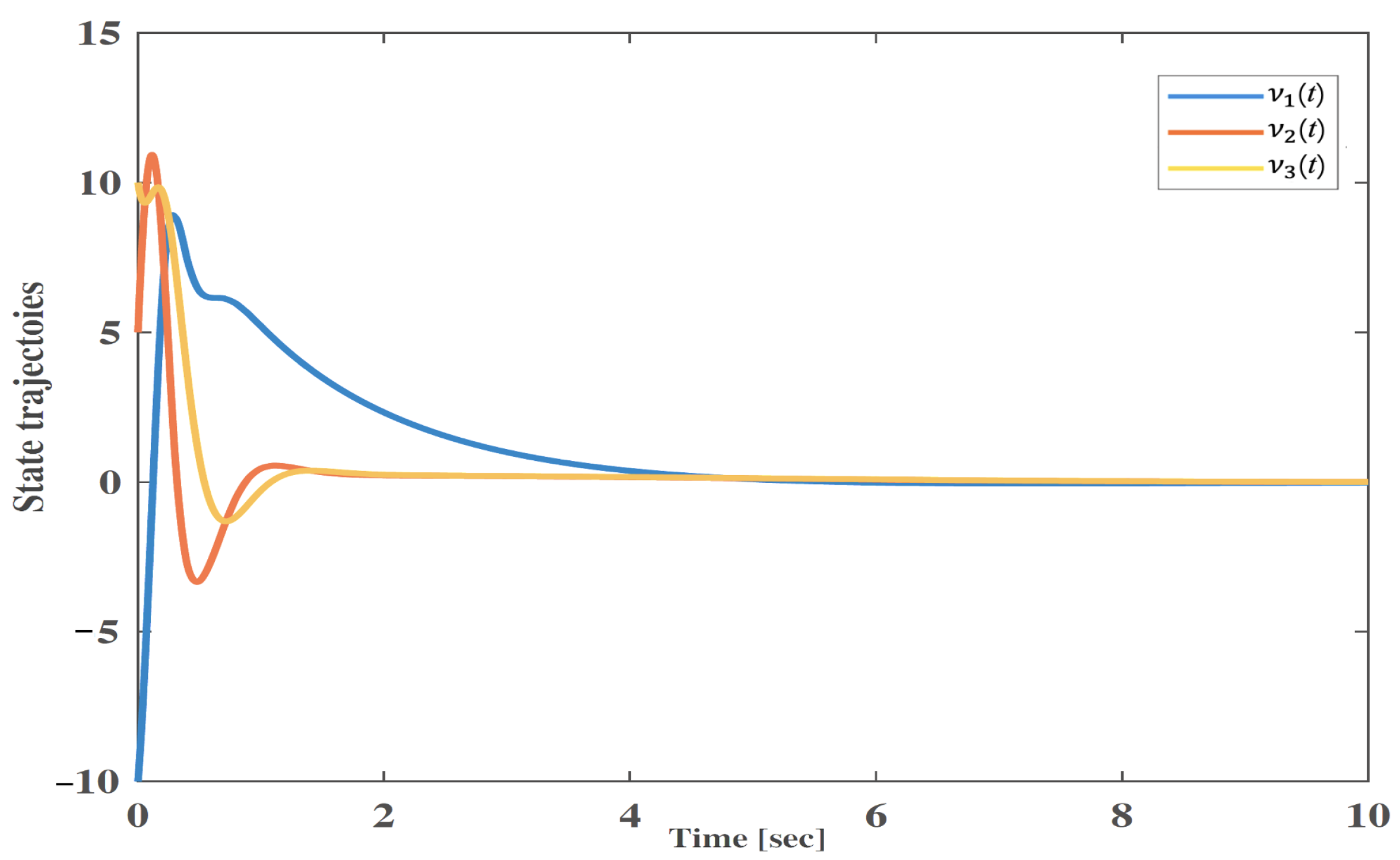
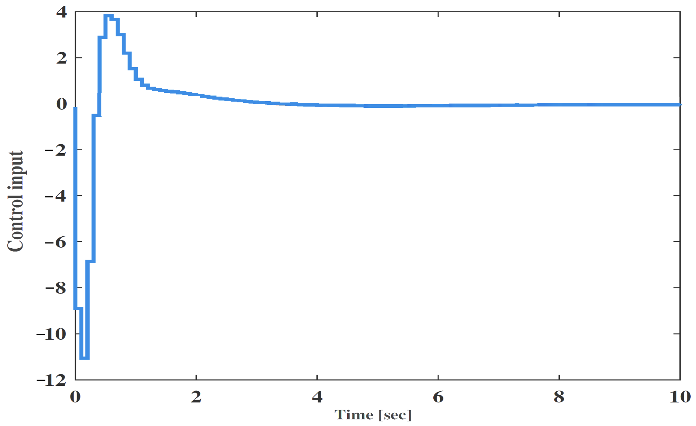
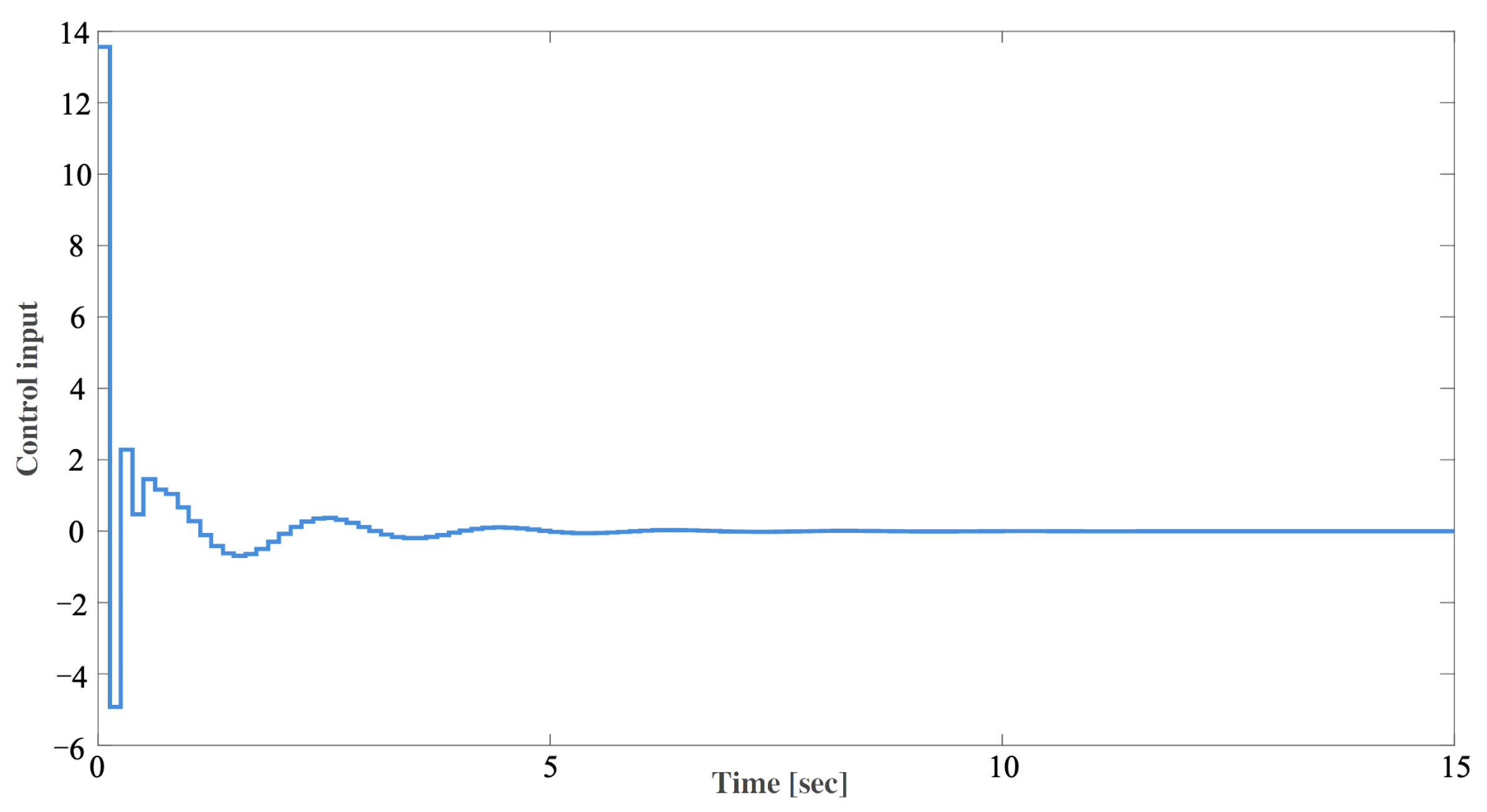
4. Numerical Validation

This section examines the model of the permanent magnet synchronous motor and the Lorenz system to highlight the merits of the proposed method.

Example 1. 

Consider the following permanent magnet synchronous motor model [28]:

$$\begin{array}{c}\hfill \left\{\begin{array}{cc}{L}_d{\displaystyle \frac{d{i}_d}{dt}}\hfill & =\left(u_d-R_1{i}_d+\overline{\omega }{L}_q{i}_q\right),\hfill \\ L_q{\displaystyle \frac{d{i}_q}{dt}}\hfill & =\left(u_q-R_1{i}_q-\overline{\omega }{L}_d{i}_d-\overline{\omega }{\psi }_r\right),\hfill \\ J{\displaystyle \frac{d\overline{\omega }}{dt}}\hfill & =\left[n_p{\psi }_r{i}_q+n_p\left(L_d-L_q\right)i_d{i}_q-T_L-\beta \overline{\omega }\right],\hfill \end{array}\right.\end{array}$$

(33)

where $i_d$ and $i_q$ represent the d-axis and q-axis currents, respectively, and $\overline{\omega }$ denotes the motor’s angular frequency. $R_1$, $T_L$, J, β, $L_d$, and $L_q$ are the stator winding resistance, the external load torque, the polar moment of inertia, the viscous damping coefficient, the d-axis, and the q-axis stator inductances, respectively. $n_p$, ${\psi }_r$, $u_d$, and $u_q$ represent the number of pole pairs, the permanent magnet flux, the stator voltage components for the d-axis, and the stator voltage components for the q-axis, respectively. Let $R_1=0.9$, $L_d=L_q=14.25$, ${\psi }_r=0.031$, $n_p=3$, $J=4.7\times {10}^{-2}$, $\beta =0.0162$. The model (33) is equivalent to the model

$$\begin{array}{c}\hfill \left\{\begin{array}{cc}{\dot{\nu }}_1\left(t\right)\hfill & =-{\displaystyle \frac{L_q}{L_d}}{\nu }_1\left(t\right)+{\nu }_2\left(t\right){\nu }_3\left(t\right)+{\overline{u}}_d,\hfill \\ {\dot{\nu }}_2\left(t\right)\hfill & =-{\nu }_2\left(t\right)-{\nu }_1\left(t\right){\nu }_3\left(t\right)+\eta {\nu }_3\left(t\right)+{\overline{u}}_q,\hfill \\ {\dot{\nu }}_3\left(t\right)\hfill & =\sigma \left({\nu }_2\left(t\right)-{\nu }_3\left(t\right)\right)+ϵ{\nu }_1\left(t\right){\nu }_2\left(t\right)-{\overline{T}}_L,\hfill \end{array}\right.\end{array}$$

(34)

where $\eta ={\displaystyle \frac{n_p{\psi }_r^2}{R_1\beta }}$, $\sigma ={\displaystyle \frac{L_q\beta }{R_{1}J}}$, ${\overline{u}}_q={\displaystyle \frac{n_p{L}_q{\psi }_r{u}_q}{R_1^2\beta }}$, ${\overline{u}}_d={\displaystyle \frac{n_p{L}_q{\psi }_r{u}_d}{R_1^2\beta }}$, $ϵ={\displaystyle \frac{L_q{\beta }^2\left(L_d-L_d\right)}{L_{d}J{n}_p{\psi }_r^2}}$, ${\overline{T}}_L={\displaystyle \frac{L_q^2{T}_L}{R_1^{2}J}}$.

Let $L_q=L_d$ and ${\nu }_3\left(t\right)\in \left[-{𝘍}_1,{𝘍}_1\right]$; using T-S fuzzy method yields

$$\dot{\nu }\left(t\right)=\sum _{i=1}^2{\Theta }_i\left(\mu \left(t\right)\right)\left(A_i\nu \left(t\right)+B_{i}u\left(t\right)+F_i\omega \left(t\right)\right),$$

(35)

where

$$\begin{array}{cc}& A_1=\left[\begin{array}{ccc}-1& {𝘍}_1& 0\\ -{𝘍}_1& -1& \eta \\ 0& \sigma & -\sigma \end{array}\right],A_2=\left[\begin{array}{ccc}-1& -{𝘍}_1& 0\\ {𝘍}_1& -1& \eta \\ 0& \sigma & -\sigma \end{array}\right],\hfill \\ & B_1=B_2=\left[\begin{array}{c}1\hfill \\ 1\hfill \\ 0\hfill \end{array}\right],F_1=F_2=\left[\begin{array}{c}0\\ 0\\ -1\end{array}\right],\hfill \\ & C_1=C_2=\left[\begin{array}{ccc}1\hfill & 0\hfill & 0\hfill \end{array}\right].\hfill \end{array}$$

Moreover, the membership functions is given as

$${\Gamma }_1(\wp \left(t\right))={\displaystyle \frac{1}{2}}\left(1+{\displaystyle \frac{{\nu }_3\left(t\right)}{{𝘍}_1}}\right),{\Gamma }_2(\wp \left(t\right))=1-{\Gamma }_1(\wp \left(t\right)).$$

Setting ${𝘍}_1=15,\widehat{\alpha }=0.5,\kappa =0.25$, $\gamma =0.01$, $\hslash =0.02$, control gains are calculated by Theorem 2 as follows.

$$K_1=[-2.7753,-0.3312,-0.0429],K_2=[-2.5583,-0.12673,-0.02195].$$

For the given $\nu \left(0\right)={\left[-10,5,10\right]}^T$, the state responses and the control input of the T-S fuzzy system are illustrated in Figure 1 and Figure 2, respectively. Figure 1 demonstrates the stability of the permanent magnet synchronous motor model, validating the effectiveness of the designed controller and the proposed methods.

Example 2. 

Consider the following nonlinear Lorenz system [29,30,31]:

$$\begin{array}{c}\hfill \left\{\begin{array}{cc}{\dot{\nu }}_1\left(t\right)\hfill & =-\alpha {\nu }_1\left(t\right)+\alpha {\nu }_2\left(t\right)+u_1\left(t\right),\hfill \\ {\dot{\nu }}_2\left(t\right)\hfill & =\phi {\nu }_1\left(t\right)-{\nu }_2\left(t\right)-{\nu }_1\left(t\right){\nu }_3\left(t\right),\hfill \\ {\dot{\nu }}_3\left(t\right)\hfill & ={\nu }_1\left(t\right){\nu }_2\left(t\right)-\beta {\nu }_3\left(t\right).\hfill \end{array}\right.\end{array}$$

(36)

The fuzzy membership functions with ${\nu }_1\left(t\right)\in [-r,r]$ are given as ${\Gamma }_1(\wp \left(t\right))={\displaystyle \frac{1}{2}}\left(1+{\displaystyle \frac{{\nu }_1\left(t\right)}{r}}\right)$ and ${\Gamma }_2(\wp \left(t\right))=1-{\Gamma }_1(\wp \left(t\right))$.

Then, the system matrices are as follows

$$A_1=\left[\begin{array}{ccc}-\alpha & \alpha & 0\\ \phi & -1& -r\\ 0& r& -\beta \end{array}\right],A_2=\left[\begin{array}{ccc}-\alpha & \alpha & 0\\ \phi & -1& r\\ 0& -r& -\beta \end{array}\right]$$

Let $\alpha =10$, $\beta ={\displaystyle \frac{8}{3}}$, $\phi =28$, $\chi =0.5$, $\rho =0.65$, and $B_1=B_2={[1,0,0]}^T$. The large sampling interval ℏ obtined by [29,30,31,32] and Corollary 1 are listed in

Table 1. The maximum sampling interval h for different methods in Example 1.

Theorem 2 [29]	Theorem 2 [30]	Theorem 2 [31]	Corollary 1 [32]	Corollary 1
0.0299	0.0347	0.0412	0.0495	0.0617

. Table 1 shows that the intervals obtained by Corollary 1 are larger than those obtained by [29,30,31,32], demonstrating the advantage of the proposed refined LLF.

Furthermore, we consider that $\chi =0.5$, $\rho =0.65$, $\hslash =0.06$, and control gain matrices by Corollary 1 are given as follows.

$$K_1=[-6.1322,-23.4452,-0.0002],K_2=[-6.1121,-24.9757,-0.0004].$$

For the given $x\left(0\right)={\left[-1,2,3\right]}^T$, the state responses and the control input of the T-S fuzzy system are given in Figure 3 and Figure 4, respectively. As shown in Figure 3, the system is achieving stability, which affirms the effectiveness of the presented controller and methodology.

5. Conclusions

This paper has addressed the sampled-data control problem for Takagi-Sugeno fuzzy systems. The refined LLF developed has included information on split sampling intervals and delayed states. Furthermore, sampling-dependent matrix functions have been presented to relax the conservativeness of the developed LLF. By employing the refined LLF, new stability and stabilization criteria for Takagi-Sugeno fuzzy systems with an $H_{\infty }$ attenuation level have been established. The derived conditions have been examined using a nonlinear permanent magnet synchronous motor and the Lorenz system, demonstrating the reduced conservatism and the effectiveness of the proposed methods.

References

1. Baillieul, J.; Antsaklis, P.J. Control and communication challenges in networked real-time systems. Proc. IEEE 2007, 95, 9–28. [Google Scholar] [CrossRef]
2. Qiu, J.; Gao, H.; Ding, S.X. Recent advances on fuzzy-model-based nonlinear networked control systems: A survey. IEEE Trans. Ind. Electr. 2015, 63, 1207–1217. [Google Scholar] [CrossRef]
3. Sun, H.; Han, H.G.; Qiao, J.F. Observer-based control for networked Takagi-Sugeno fuzzy systems with stochastic packet losses. Inf. Sci. 2023, 644, 119275. [Google Scholar] [CrossRef]
4. Xue, W.; Jin, Z.; Tian, Y. Finite-time fault-tolerant control of nonlinear spacecrafts with randomized actuator fault: Fuzzy model approach. Symmetry 2024, 16, 873. [Google Scholar] [CrossRef]
5. Niu, Y.; Xu, X.; Liu, M. Fixed time synchronization of stochastic Takagi-Sugeno fuzzy recurrent neural net-works with distributed delay under feedback and adaptive controls. Axioms 2024, 13, 391. [Google Scholar] [CrossRef]
6. Castorena, G.A.H.; Mendez, G.M.; Lopez-Juarez, I.; Garcia, M.A.A.; Artinez-Peon, D.C.; Mon-tes-Dorantes, P.N. Parameter prediction with novel enhanced wagner hagras interval type-3 Takagi-Sugeno-Kang fuzzy system with type-1 non-singleton inputs. Mathematics 2024, 12, 1976. [Google Scholar] [CrossRef]
7. Lee, D.H.; Kim, Y.J.; Lee, S.H.; Kwon, O.M. Enhancing stability criteria for linear systems with interval time-Varying delays via augmented Lyapunov-Krasovskii functional. Mathematics 2024, 12, 2241. [Google Scholar] [CrossRef]
8. Wang, X.; Park, J.H.; She, K.; Zhong, S.M.; Shi, L. Stabilization of chaotic systems with T-S fuzzy model and nonuniform sampling: A switched fuzzy control approach. IEEE Trans. Fuzzy Syst. 2018, 27, 1263–1271. [Google Scholar] [CrossRef]
9. Tseng, C.S.; Chen, B.S.; Uang, H.J. Fuzzy tracking control design for nonlinear dynamic systems via TS fuzzy model. IEEE Trans. Fuzzy Syst. 2001, 9, 381–392. [Google Scholar] [CrossRef]
10. Zhao, X.Y.; Chang, X.H. H filtering for nonlinear discrete-time singular systems in encrypted state. Neur. Proc. Lett. 2023, 55, 2843–2866. [Google Scholar] [CrossRef]
11. Rhee, B.J.; Won, S. A new fuzzy Lyapunov function approach for a Takagi-Sugeno fuzzy control system design. Fuzzy Sets Syst. 2006, 157, 1211–1228. [Google Scholar] [CrossRef]
12. Wang, X.Y.; Chang, X.H. Nonlinear continuous-time system H control based on dynamic quantization and event-triggered mechanism. Neur. Proc. Lett. 2023, 55, 12223–12238. [Google Scholar] [CrossRef]
13. Zhao, N.; Zhao, X.; Zong, G.; Xu, N. Resilient event-triggered filtering for networked switched T-S fuzzy systems under denial-of-service attacks. IEEE Trans. Fuzzy Syst. 2024, 32, 2140–2152. [Google Scholar] [CrossRef]
14. Tan, Y.; Yuan, Y.; Xie, X.; Niu, B. Dynamic event-triggered security control for networked T-S fuzzy system with non-uniform sampling. Fuzzy Sets Syst. 2023, 452, 91–109. [Google Scholar] [CrossRef]
15. Yang, T.; Zou, R.; Liu, F.; Liu, C.; Sidorov, D. Improved stabilization condition of delayed T-S fuzzy systems via an extended quadratic function negative-determination lemma. Chaos Solitons Fractals 2023, 175, 114055. [Google Scholar] [CrossRef]
16. An, J.H.; Kim, H.S. Interval type-2 duzzy-model-based sampled-data control of an AUV depth system with input saturation. Actuators 2024, 13, 71. [Google Scholar] [CrossRef]
17. Zheng, M.; Su, Y.; Yan, C. Further stability criteria for sampled-data-based dynamic positioning ships using Takagi-Sugeno fuzzy models. Symmetry 2024, 16, 108. [Google Scholar] [CrossRef]
18. Dhanya, V.; Arunkumar, A.; Chaisena, K. Sampled-data based fault-tolerant control design for uncertain CE151 helicopter system with random delays: Takagi-Sugeno fuzzy approach. Fractal Fract. 2022, 6, 498. [Google Scholar] [CrossRef]
19. Chen, T.; Francis, B.A. Optimal Sampled-Data Control Systems; Springer Science & Business Media: New York, NY, USA, 2012. [Google Scholar]
20. Arthanari, S.; Joo, Y.H. Memory sampled-data control for T-S fuzzy-based permanent magnet synchronous generator via an improved looped functional. IEEE Trans. Syst. Man Cybern Syst. 2023, 53, 4417–4428. [Google Scholar] [CrossRef]
21. Xu, X.; Wang, L.; Du, Z.; Kao, Y. H sampled-data control for uncertain fuzzy systems under Markovian jump and FBm. Appl. Math. Comput. 2023, 451, 128014. [Google Scholar] [CrossRef]
22. Wang, X.; Park, J.H.; Yang, H.; Zhao, G.; Zhong, S. An improved fuzzy sampled-data control to stabilization of T-S fuzzy systems with state delays. IEEE Trans. Cybern. 2020, 50, 3125–3135. [Google Scholar] [CrossRef] [PubMed]
23. Qiu, Y.; Hua, C.; Wang, Y. Nonfragile sampled-data control of T-S fuzzy systems with time delay. IEEE Trans. Fuzzy Syst. 2021, 30, 3202–3210. [Google Scholar] [CrossRef]
24. Ge, C.; Shi, Y.; Park, J.H.; Hua, C. Robust H stabilization for T-S fuzzy systems with time-varying delays and memory sampled-data control. Appl. Math. Comput. 2019, 346, 500–512. [Google Scholar] [CrossRef]
25. Liu, Y.; Park, J.H.; Guo, B.; Shu, Y. Further results on stabilization of chaotic systems based on fuzzy memory sampled-data control. IEEE Trans. Fuzzy Syst. 2018, 26, 1040–1045. [Google Scholar] [CrossRef]
26. Zeng, H.B.; Teo, K.L.; He, Y.; Wang, W. Sampled-data stabilization of chaotic systems based on a T-S fuzzy model. Inf. Sci. 2019, 483, 262–272. [Google Scholar] [CrossRef]
27. Zhang, R.; Zeng, D.; Park, J.H.; Lam, H.K.; Xie, X. Fuzzy sampled-data control for synchronization of T-S fuzzy reaction-diffusion neural networks with additive time-varying delays. IEEE Trans. Cybern. 2020, 251, 2384–2397. [Google Scholar] [CrossRef]
28. Shanmugam, L.; Joo, Y.H. Design of interval type-2 fuzzy-based sampled-data controller for nonlinear sys-tems using novel fuzzy Lyapunov functional and its application to PMSM. IEEE Trans. Syst. Man Cybern. 2021, 51, 542–551. [Google Scholar] [CrossRef]
29. Zhu, X.L.; Chen, B.; Yue, D.; Wang, Y. An improved input delay approach to stabilization of fuzzy systems under variable sampling. IEEE Trans. Fuzzy Syst. 2012, 20, 330–341. [Google Scholar] [CrossRef]
30. Wu, Z.G.; Shi, P.; Su, H.; Chu, J. Sampled-data fuzzy control of chaotic systems based on a T-S fuzzy model. IEEE Trans. Fuzzy Syst. 2013, 22, 153–163. [Google Scholar] [CrossRef]
31. Wang, Z.P.; Wu, H.N. On fuzzy sampled-data control of chaotic systems via a time-dependent Lyapunov functional approach. IEEE Trans. Cybern. 2014, 45, 819–829. [Google Scholar] [CrossRef]
32. Shanmugam, L.; Joo, Y.H. Stability criteria for fuzzy-based sampled-data control systems via a fractional parameter-based refined looped Lyapunov functional. IEEE Trans. Fuzzy Syst. 2022, 30, 2538–2549. [Google Scholar] [CrossRef]
33. Sheng, Z.; Xu, S. A sampled-data control method related to time for Takagi-Sugeno fuzzy systems via novel sampling-dependent functional approach. IEEE Trans. Fuzzy Syst. 2024, 31, 460–469. [Google Scholar] [CrossRef]
34. Essiambre, R.J.; Tkach, R.W. Capacity trends and limits of optical communication networks. Proc. IEEE 2012, 100, 1035–1055. [Google Scholar] [CrossRef]
35. Seuret, A. A novel stability analysis of linear systems under asynchronous samplings. Automatica 2012, 48, 177–182. [Google Scholar] [CrossRef]
36. Oncoy, D.J.; Cardim, R.; Teixeira, M.C.; Faria, F.A.; Assuncao, E.; Lazarini, A.Z. New stabilization conditions for fuzzy-based sampled-data control systems using a fuzzy Lyapunov functional. IEEE Access 2023, 11, 15390–15403. [Google Scholar] [CrossRef]
37. Zeng, H.B.; Teo, K.L.; He, Y. A new looped-functional for stability analysis of sampled-data systems. Automatica 2017, 82, 328–331. [Google Scholar] [CrossRef]
38. Park, J.; Park, P. An extended looped-functional for stability analysis of sampled-data systems. Int. J. Robust Nonlinear Control 2020, 30, 7962–7969. [Google Scholar] [CrossRef]
39. Guan, C.; Fei, Z.; Park, P. Modified looped functional for sampled-data control of T-S fuzzy Markovian jump systems. IEEE Trans. Fuzzy Syst. 2021, 29, 2543–2552. [Google Scholar] [CrossRef]
40. Park, J.; Park, P. A less conservative stability criterion for sampled-data system via a fractional-delayed state and its state-space model. Int. J. Robust Nonlinear Control 2021, 29, 2561–2572. [Google Scholar] [CrossRef]
41. Zhang, X.M.; Han, Q.L.; Ge, X.; Ning, B.; Zhang, B.L. Sampled-data control systems with non-uniform sampling: A survey of methods and trends. Annu. Rev. Control 2023, 55, 70–91. [Google Scholar] [CrossRef]
42. Liu, K.; Fridman, E. Networked-based stabilization via discontinuous Lyapunov functionals. Int. J. Robust Nonlinear Control 2012, 22, 420–436. [Google Scholar] [CrossRef]
43. Lee, T.H.; Park, J.H. Stability analysis of sampled-data systems via free-matrix-based time-dependent dis-continuous Lyapunov approach. IEEE Trans. Autom. Control 2017, 62, 3653–3657. [Google Scholar] [CrossRef]
44. Wang, J.; Zhang, H.; Wang, Z. Sampled-data synchronization for complex networks based on discontinuous LKF and mixed convex combination. J. Franklin Inst. 2015, 352, 4741–4757. [Google Scholar] [CrossRef]
45. Seuret, A.; Gouaisbaut, F. Wirtinger-based integral inequality: Application to time-delay systems. Automatica 2013, 30, 2860–2866. [Google Scholar] [CrossRef]
46. Zeng, H.B.; He, Y.; Wu, M.; She, J. Free-matrix-based integral inequality for stability analysis of systems with time-varying delay. IEEE Trans. Autom. Control 2015, 60, 2768–2772. [Google Scholar] [CrossRef]
47. Seuret, A.; Gouaisbaut, F. Stability of linear systems with time-varying delays using Bessel-Legendre ine-qualities. IEEE Trans. Autom. Control 2018, 63, 225–232. [Google Scholar] [CrossRef]
48. Wang, L.; Lam, H. New stability criterion for continuous-time Takagi-Sugeno fuzzy systems with time-varying delay. IEEE Trans. Cybern. 2019, 49, 1551–1556. [Google Scholar] [CrossRef]
Figure 1. State trajectoies of Example 1.
Symmetry 16 01119 g001
Figure 2. Control input of Example 1.
Symmetry 16 01119 g002
Figure 3. State trajectoies of Example 2.
Symmetry 16 01119 g003
Figure 4. Control input of Example 2.
Symmetry 16 01119 g004