Comparative Analysis of Influenza Modeling Using Novel Fractional Operators with Real Data

Abstract

In this work, the efficacy of fractional models under Atangana–Baleanu–Caputo, Caputo–Fabrizio, and Caputo is compared to the performance of integer-order models in the forecasting of weekly influenza cases using data from the Kingdom of Saudi Arabia. The suggested fractional influenza model was effectively verified using fractional calculus. Our investigation uncovered the topic’s essential properties and deepened our understanding of disease progression. Furthermore, we analyzed the numerical scheme’s positivity, limitations, and symmetry. The fractional-order models demonstrated superior accuracy, producing smaller root mean square error (RMSE) and mean absolute error (MAE) than the classical model. The novelty of this work lies in introducing the Atangana–Baleanu–Caputo fractional model to influenza forecasting to incorporate memory of an epidemic, which leads to higher accuracy than traditional models. These models effectively captured the peak and drop of influenza cases. Based on these findings, it can be concluded that fractional-order models perform better than typical integer-order models when predicting influenza dynamics. These insights should illuminate the importance of fractional calculus in addressing epidemic threats.

1. Introduction

Different types of influenza viruses cause respiratory infections, commonly known as influenza [1,2]. The most common method of transmitting these viruses is through respiratory droplets. They are very infectious. The three primary types of influenza viruses are A, B, and C. Type A is more prevalent among mammalian animals, type B mainly affects humans, and type C typically causes moderate respiratory problems. Type A is the most common form [3,4]. Researchers need help formulating models since these models play a significant and crucial role in describing phenomena occurring worldwide in various sectors, including science, engineering, and technology [5].

It has been demonstrated that the study of fractional models is an adaptable topic that has been successful in various scientific fields [6,7]. Because diseases, particularly infectious diseases, significantly impact people’s lives, it is essential to study and identify ways to combat them, whether by pharmaceutical means or non-pharmaceutical practices, to manage and forecast them in the future [8,9].

Mathematicians and academics are considering several different mathematical models to understand the dynamics of the infectious disease influenza. Researchers conduct this analysis to understand the disease better. An example of this would be the mathematical model [10], which investigates the influenza model. The authors of [11] consider a model of an avian influenza epidemic and provide control measures for the virus’s elimination. The writers briefly outlined the dynamics of the human and bird populations. For model fitting, the authors of [12] considered both the human influenza model and the actual cases. In [13], the researchers investigate a mathematical model that describes the vaccine resistance mechanism for the dynamics of an influenza virus. Article [14] takes into consideration a model of influenza that has a nonlinear incidence rate. The authors covered various discussions and methods regarding how to control the infection. All of the models presented earlier for influenza and their controls are restricted to integer orders only, and only one method can be used to perform their numerical calculations. Because they generalize the integer situation, fractional models are more valuable than classical models. Additionally, one can have a significant amount of information regarding the model’s heredity and memory.

The fractional influenza illness is presented in [15], and a fractional influenza epidemiological model is provided in [16]. This fractional HPAI model is provided in reference [17]. In [18], a fractional model of visceral leishmaniasist uses the ABC and Cf operators. In addition, the ABC operator has been successfully applied to epidemiological models and other fields, as evidenced by the references [19,20,21,22]. In addition, some recent significant results published regarding fractional calculus and its application to situations that occur in the real world can be found in [23,24]. The writers of these recently released works discussed various issues associated with science and engineering and produced helpful results regarding these issues [25,26,27].

Recent studies on influenza have investigated the influenza spread and specified the necessity of using a fractional-order approach to modeling [28,29,30,31,32,33,34]. Models with fractional derivatives provide the ability to remember and inherit the processes of virus transmission and provide better fits to the data. This is particularly important in enhancing the level of forecasting accuracy and predicting future trends of the flu epidemic, which is vital in policy-making in the management of epidemics.

This work’s main contribution is its assessment of the efficacy of the fractal models, specifically the Caputo, CF, ABC operator, and classical models, in the context of influenza dynamics. This research is distinguished by its rigorous assessment of the fractal models, particularly the ABC model, and its demonstration of its superiority over the other two models in epidemiological modeling.

The novelty of this work lies in using the ABC operator, which performed better than the models using the classical, Caputo, and CF operators. Furthermore, the ABC operator has shown greater accuracy in reflecting accurate data, with a lower relative error.

The structure of this work is summarized as follows: Section 2 begins with an introduction to the preliminary concepts utilized in our research. Section 3 and Section 4 present the development of the model in terms of the classical and fractional meanings, respectively. Section 5 discusses the model’s analysis. Section 6 presents the numerical findings and explanations. Section 7 presents the study’s results and conclusions.

2. Preliminaries

Definition 1

([35]). The (RL) integral $u:{\mathbb{R}}^{+}\to \mathbb{R}$ with order $\alpha >0$ is given by

$$I_{0^{+}}^{\alpha }\left(u\left(t\right)\right)={\displaystyle \frac{1}{\Gamma \left(\alpha \right)}}{\int }_0^t{(t-s)}^{\alpha -1}u\left(s\right)ds,t>0,$$

(1)

Definition 2

([35]). The RL differential operator for $u\left(t\right)$, $\alpha >0$ is given by

$${\mathbb{D}}_{0^{+}}^{\alpha }\left(u\left(t\right)\right)={\displaystyle \frac{1}{\Gamma (m-\alpha )}}{\displaystyle \frac{d^m}{d{t}^m}}\left({\int }_0^t{(t-s)}^{m-\alpha -1}u\left(s\right)ds\right),t>0,$$

(2)

where $m-1<\alpha <m$, $m\in \mathbb{N}$.

Definition 3

([35]). The Caputo definition with $\alpha >0$ is given by

$${}^C\mathbb{D}_{0^{+}}^{\alpha }\left(u\left(t\right)\right)={\displaystyle \frac{1}{\Gamma (m-\alpha )}}{\int }_0^t{(t-s)}^{m-\alpha -1}{u}^{\left(m\right)}\left(s\right)ds,t>0,$$

(3)

where $m-1<\alpha <m$, $m\in \mathbb{N}$.

Definition 4

([36]). The CF operator of order α, where $\alpha \in [0, 1]$, is defined as follows:

$${}^{CF}\mathbb{D}_{0^{+}}^{\alpha }\left(u\left(t\right)\right)={\displaystyle \frac{M\left(\alpha \right)}{1-\alpha }}{\int }_0^{t}exp\left[-{\displaystyle \frac{\alpha }{1-\alpha }}(t-s)\right]u^{\prime }\left(s\right)ds,t>0,$$

(4)

where $M\left(\alpha \right)$ is a normalization function, $M\left(0\right)=M\left(1\right)=1$, and $\alpha \in [0, 1]$.

Definition 5

([37]). Let $u\left(t\right)\in H^1(0, T)$, $T>0$, and $\alpha \in (0, 1]$, then the ABC operator under Caputo sense given by

$${}^{ABC}\mathbb{D}_{0^{+}}^{\alpha }\left(u\left(t\right)\right)={\displaystyle \frac{B\left(\alpha \right)}{1-\alpha }}{\int }_0^t{E}_{\alpha }\left[-{\displaystyle \frac{\alpha }{1-\alpha }}(t-s)\right]u^{\prime }\left(s\right)ds,$$

(5)

where $B\left(\alpha \right)={\displaystyle \frac{M\left(\alpha \right)}{M\left(1\right)}}=1$ and $E_{\alpha }(·)$ is the Mittag–Leffler function.

Definition 6

([38]). The CF operator under Caputo sense, then the integral equation is given by

$$I_{0^{+}}^{\alpha }\left(u\left(t\right)\right)={\displaystyle \frac{2}{M\left(\alpha \right)}}{\int }_0^{t}u\left(s\right)ds.$$

(6)

Definition 7

([37]). The ABC operator under Caputo sense, then the integral equation is given by

$${}^{ABC}I_{0^{+}}^{\alpha }\left(u\left(t\right)\right)={\displaystyle \frac{B\left(\alpha \right)}{1-\alpha }}{\int }_0^t{E}_{\alpha }\left[-{\displaystyle \frac{\alpha }{1-\alpha }}(t-s)\right]u\left(s\right)ds.$$

(7)

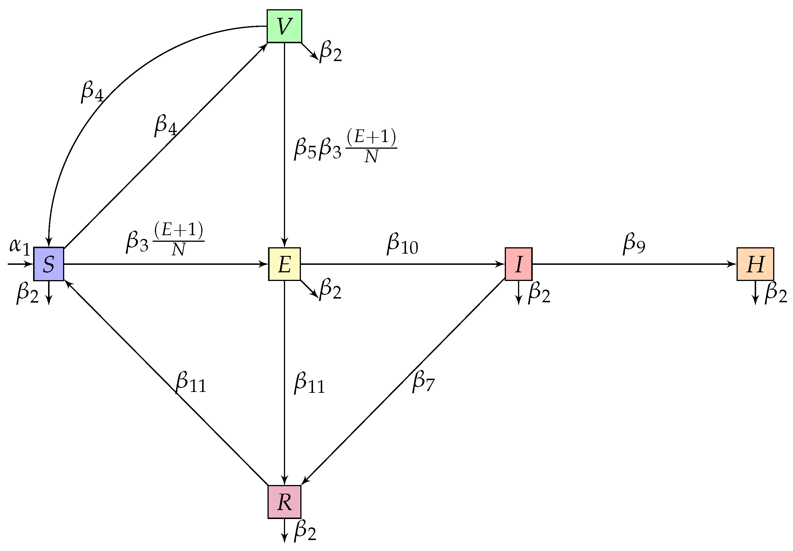
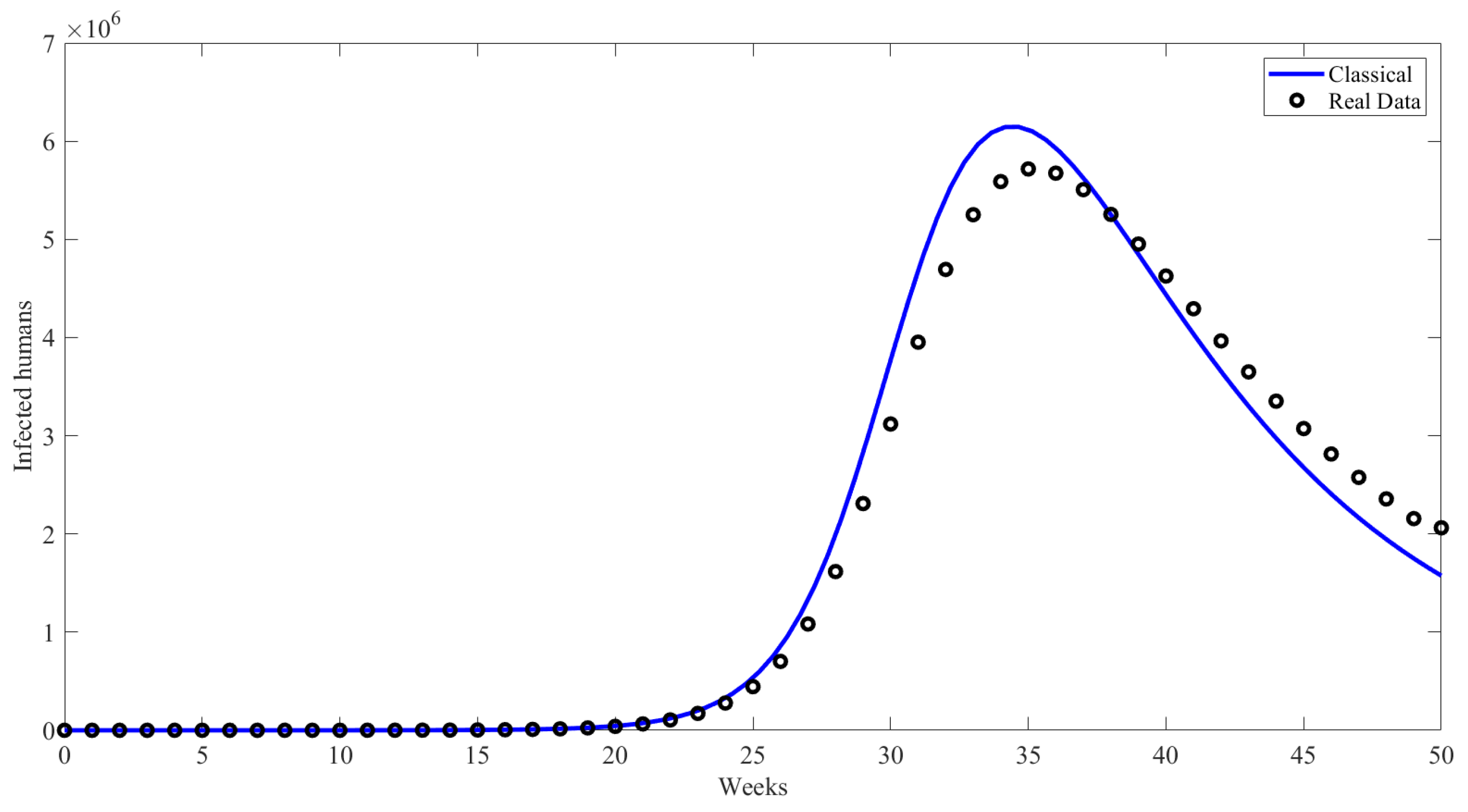
3. The Development of the Model in the Classical Meaning

The transmission dynamics of influenza are represented using the SEIHR-V model. This model consists of compartments for individuals who are (S), (E), (I), (H), (R), and (V): susceptible, exposed, infectious, hospitalized, recovered, and vaccinated (referred to as the $SEIHR-V$ model). At each given moment, t, then,

$$N\left(t\right)=V\left(t\right)+E\left(t\right)+I\left(t\right)+H\left(t\right)+R\left(t\right)+S\left(t\right).$$

Every class experiences a constant natural mortality rate of ${\beta }_2$. The S is supposed to expand through recruiting mechanisms at a rate of ${\beta }_1$ and through declining immunity of persons in R and V at ${\beta }_{11}$. It is reduced through vaccination at a rate of ${\beta }_4$.

$$f_1={\beta }_3{\displaystyle \frac{(E+I)S}{N}},$$

The variable ${\beta }_5$ represents the ineffectiveness of vaccination, which may be expressed as the difference between ${\beta }_3$ and ${\beta }_5$. On the other hand, ${\beta }_3$ represents the likelihood of an individual belonging to class V or S.

At the rate of ${\beta }_4$, individuals from class S are recruited to become members of class V. It is impossible to obtain long-lasting immunity by vaccination nor to ensure complete protection. Therefore, persons vaccinated become vulnerable once more at a rate of ${\beta }_{11}$ owing to the fact that their immunity is diminishing and they are exposed to the virus due to the force of infection.

$$f_2={\beta }_5{\beta }_3{\displaystyle \frac{(E+I)V}{N}}.$$

Class E individuals are recruited by illnesses $f_1$ and $f_2$, progress to class I at w, and reach class R at ${\beta }_8$. Infected people from class E are recruited at rate ${\beta }_{10}$, recover at ${\beta }_7$, and spend a percentage of time in the hospital, $ϵ$. The R increases from classes $E,I,$ and H at rates ${\beta }_8,{\beta }_7$, and ${\beta }_9$, respectively, and becomes vulnerable again at ${\beta }_{11}$. Based on the given description, we formulate a system (8) of ordinary differential equations to represent the model formally.

$$\begin{array}{ccc}\hfill {\displaystyle \frac{dS}{dt}}& =& {\beta }_1+{\beta }_{11}(V+R)-{\beta }_3{\displaystyle \frac{(E+I)S}{N}}-({\beta }_4+{\beta }_2)S\hfill \\ \hfill {\displaystyle \frac{dV}{dt}}& =& {\beta }_{4}S-{\beta }_5{\beta }_3{\displaystyle \frac{(E+I)V}{N}}-({\beta }_{11}+{\beta }_2)V\hfill \\ \hfill {\displaystyle \frac{dE}{dt}}& =& {\beta }_3{\displaystyle \frac{(E+I)(S+{\beta }_{5}V)}{N}}-({\beta }_{10}+{\beta }_8+{\beta }_2)E\hfill \\ \hfill {\displaystyle \frac{dI}{dt}}& =& {\beta }_{10}E-({\beta }_7+ϵ+{\beta }_2)I\hfill \\ \hfill {\displaystyle \frac{dH}{dt}}& =& ϵI-({\beta }_9+{\beta }_2)H\hfill \\ \hfill {\displaystyle \frac{dR}{dt}}& =& {\beta }_{8}E+{\beta }_{7}I+{\beta }_{9}H-({\beta }_{11}+{\beta }_2)R,\hfill \end{array}$$

(8)

with initial conditions $R_0\ge 0, H_0\ge 0, I_0\ge 0, E_0\ge 0, V_0\ge 0,$ and $S_0\ge 0.$ 

Table 1. Description of compartments in model (8).

Compartment	Description
S	Susceptible class
V	Vaccinated class
E	Exposed class
I	Infected class
H	Hospitalized class
R	Recovered class

and

Table 2. Explanation of the model’s parameters (8).

Parameter	Description	Value	Source
${\beta }_1$	Population recruitment rate	${10}^4$	[39]
${\beta }_2$	Natural death rate	0.000254 weeks−1	[39]
${\beta }_3$	Average effective contact rate	0.858	Fitted
${\beta }_4$	Vaccination rate	0.114	Fitted
${\beta }_5$	Vaccine inefficacy	1	Fitted
${\beta }_6$	Average hospitalization rate	0.0015	Fitted
${\beta }_7$	Recovery rate for infected class	0.385 day−1	[40]
${\beta }_8$	Recovery rate for exposed class	0.34	Fitted
${\beta }_9$	Recovery rate for hospitalized individuals	0.68	Fitted
${\beta }_{10}$	Average latent or incubation period	0.625 day−1	[41]
${\beta }_{11}$	Rate at which individuals lose immunity	0.0067 day−1	[39]

provides a full description of the model parameters, and Figure 1 shows the transfer diagram of the model.

Table 1 and Table 2 display detailed explanations, precise values, and comprehensive information regarding all model parameters. Influenza statistics were for 2021 from Saudi Arabia [39] and used the MCMC method to fit Model (8), which is described in Table 1; the parameters are displayed in Table 2.

4. The Development of the Model in the Fractional Meaning

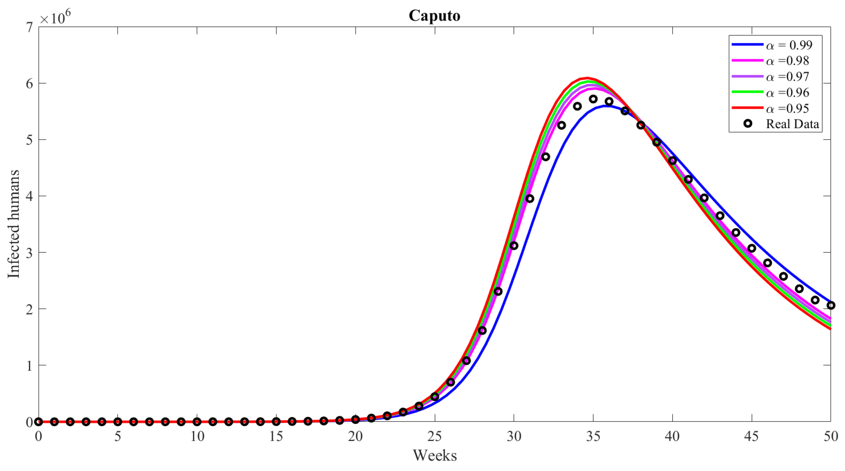
This section presents the fractional influenza model, which utilizes six differential equations. The description of fractional models, which are memory-based systems, necessitates using numerous methods. Scientists in biology, physics, and engineering have noted that fractional-order models can make more precise predictions of experimental outcomes compared to their integer-order counterparts [38,42,43,44].

$$\begin{array}{ccc}\hfill {}^{*}\mathcal{D}_{0,t}^{\alpha }S\left(t\right)& =& {\beta }_1+{\beta }_{11}(V+R)-{\beta }_3{\displaystyle \frac{(E+I)S}{N}}-({\beta }_4+{\beta }_2)S\hfill \\ \hfill {}^{*}\mathcal{D}_{0,t}^{\alpha }V\left(t\right)& =& {\beta }_{4}S-{\beta }_5{\beta }_3{\displaystyle \frac{(E+I)V}{N}}-({\beta }_{11}+{\beta }_2)V\hfill \\ \hfill {}^{*}\mathcal{D}_{0,t}^{\alpha }E\left(t\right)& =& {\beta }_3{\displaystyle \frac{(E+I)(S+{\beta }_{5}V)}{N}}-({\beta }_{10}+{\beta }_8+{\beta }_2)E\hfill \\ \hfill {}^{*}\mathcal{D}_{0,t}^{\alpha }I\left(t\right)& =& {\beta }_{10}E-({\beta }_7+ϵ+{\beta }_2)I\hfill \\ \hfill {}^{*}\mathcal{D}_{0,t}^{\alpha }H\left(t\right)& =& {\beta }_{6}I-({\beta }_9+{\beta }_2)H\hfill \\ \hfill {}^{*}\mathcal{D}_{0,t}^{\alpha }R\left(t\right)& =& {\beta }_{8}E+{\beta }_{7}I+{\beta }_{9}H-({\beta }_{11}+{\beta }_2)R,\hfill \end{array}$$

(9)

where * is a fractional-order operator. Table 2 provides full description parameters and Figure 1 shows the transfer diagram.

4.1. Caputo Meaning

Here, we present the fractional influenza model under the Caputo operator.

$$\begin{array}{ccc}\hfill {}^C\mathcal{D}_{0,t}^{\alpha }S\left(t\right)& =& {\beta }_1+{\beta }_{11}(V+R)-{\beta }_3{\displaystyle \frac{(E+I)S}{N}}-({\beta }_4+{\beta }_2)S\hfill \\ \hfill {}^C\mathcal{D}_{0,t}^{\alpha }V\left(t\right)& =& {\beta }_{4}S-{\beta }_5{\beta }_3{\displaystyle \frac{(E+I)V}{N}}-({\beta }_{11}+{\beta }_2)V\hfill \\ \hfill {}^C\mathcal{D}_{0,t}^{\alpha }E\left(t\right)& =& {\beta }_3{\displaystyle \frac{(E+I)(S+{\beta }_{5}V)}{N}}-({\beta }_{1}0+{\beta }_8+{\beta }_2)E\hfill \\ \hfill {}^C\mathcal{D}_{0,t}^{\alpha }I\left(t\right)& =& {\beta }_{1}0E-({\beta }_7+ϵ+{\beta }_2)I\hfill \\ \hfill {}^C\mathcal{D}_{0,t}^{\alpha }H\left(t\right)& =& ϵI-({\beta }_9+{\beta }_2)H\hfill \\ \hfill {}^C\mathcal{D}_{0,t}^{\alpha }R\left(t\right)& =& {\beta }_{8}E+{\beta }_{7}I+{\beta }_{9}H-({\beta }_{11}+{\beta }_2)R,\hfill \end{array}$$

(10)

4.2. Caputo–Fabrizio Meaning

Here, we present the fractional model under the CF operator.

$$\begin{array}{ccc}\hfill {}^{CF}\mathcal{D}_{0,t}^{\alpha }S\left(t\right)& =& {\beta }_1+{\beta }_{11}(V+R)-{\beta }_3{\displaystyle \frac{(E+I)S}{N}}-({\beta }_4+{\beta }_2)S\hfill \\ \hfill {}^{CF}\mathcal{D}_{0,t}^{\alpha }V\left(t\right)& =& {\beta }_{4}S-{\beta }_5{\beta }_3{\displaystyle \frac{(E+I)V}{N}}-({\beta }_{11}+{\beta }_2)V\hfill \\ \hfill {}^{CF}\mathcal{D}_{0,t}^{\alpha }E\left(t\right)& =& {\beta }_3{\displaystyle \frac{(E+I)(S+{\beta }_{5}V)}{N}}-({\beta }_{1}0+{\beta }_8+{\beta }_2)E\hfill \\ \hfill {}^{CF}\mathcal{D}_{0,t}^{\alpha }I\left(t\right)& =& {\beta }_{1}0E-({\beta }_7+ϵ+{\beta }_2)I\hfill \\ \hfill {}^{CF}\mathcal{D}_{0,t}^{\alpha }H\left(t\right)& =& ϵI-({\beta }_9+{\beta }_2)H\hfill \\ \hfill {}^{CF}\mathcal{D}_{0,t}^{\alpha }R\left(t\right)& =& {\beta }_{8}E+{\beta }_{7}I+{\beta }_{9}H-({\beta }_{11}+{\beta }_2)R,\hfill \end{array}$$

(11)

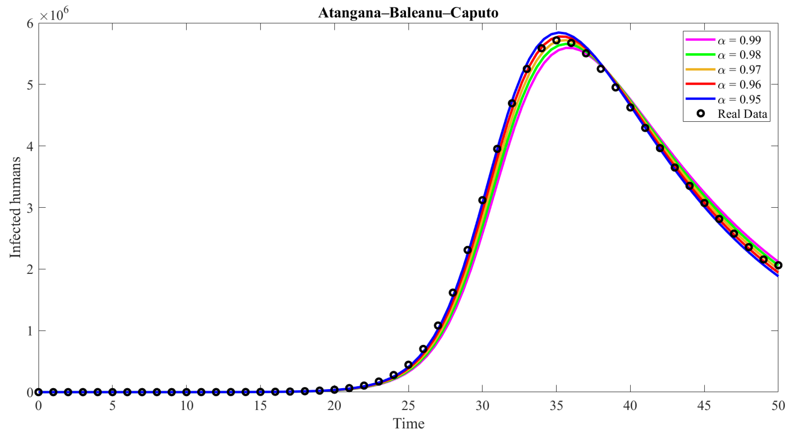
4.3. Atangana–Baleanu–Caputo Meaning

Here, we present the fractional model under the ABC operator.

$$\begin{array}{ccc}\hfill {}^{ABC}\mathcal{D}_{0,t}^{\alpha }S\left(t\right)& =& {\beta }_1+{\beta }_{11}(V+R)-{\beta }_3{\displaystyle \frac{(E+I)S}{N}}-({\beta }_4+{\beta }_2)S\hfill \\ \hfill {}^{ABC}\mathcal{D}_{0,t}^{\alpha }V\left(t\right)& =& {\beta }_{4}S-{\beta }_5{\beta }_3{\displaystyle \frac{(E+I)V}{N}}-({\beta }_{11}+{\beta }_2)V\hfill \\ \hfill {}^{ABC}\mathcal{D}_{0,t}^{\alpha }E\left(t\right)& =& {\beta }_3{\displaystyle \frac{(E+I)(S+{\beta }_{5}V)}{N}}-({\beta }_{1}0+{\beta }_8+{\beta }_2)E\hfill \\ \hfill {}^{ABC}\mathcal{D}_{0,t}^{\alpha }I\left(t\right)& =& {\beta }_{1}0E-({\beta }_7+ϵ+{\beta }_2)I\hfill \\ \hfill {}^{ABC}\mathcal{D}_{0,t}^{\alpha }H\left(t\right)& =& ϵI-({\beta }_9+{\beta }_2)H\hfill \\ \hfill {}^{ABC}\mathcal{D}_{0,t}^{\alpha }R\left(t\right)& =& {\beta }_{8}E+{\beta }_{7}I+{\beta }_{9}H-({\beta }_{11}+{\beta }_2)R,\hfill \end{array}$$

(12)

5. Analysis of the Model

This section explores the dynamical elements of model (8) to determine the conditions for disease persistence or extinction in a population.

5.1. Disease-Free Equilibrium Point $\left(E_{dfe}\right)$

If there is no influenza, all the infected model compartments remain unaffected, meaning that the values of E, I, H, and R are all equal to zero. The $\left(E_{dfe}\right)$ coordinates of system (8) are determined by setting Equation (8) to zero, as shown below:

$$E_{dfe}=\left(S_0^{*}, V_0^{*}, E_0^{*}, I_0^{*}, H_0^{*}, R_0^{*}\right),$$

(13)

where $S_0^{*}={\displaystyle \frac{{\beta }_1({\beta }_{11}+{\beta }_2)}{{\beta }_2({\beta }_4+{\beta }_{11}+{\beta }_2)}}, V_0^{*}={\displaystyle \frac{{\beta }_4{\beta }_1}{{\beta }_2({\beta }_4+{\beta }_{11}+{\beta }_2)}}$, and $E_0^{*}=I_0^{*}=H_0^{*}=R_0^{*}=0.$

5.2. Positivity and Boundedness

Theorem 1.

If the initial values $\left(S_0, V_0, E_0, I_0, H_0, R_0\right)$ are non-negative, then the solutions $\left(S, V, E, I, H, R\right)$ of the model (8) are positive for all $t>0$.

Proof. 

By substituting

$$S=0, V=0, E=0, I=0, H=0, R=0$$

into the equations of system (8), respectively in order, we have

$$\begin{array}{ccc}\hfill {\left.{\displaystyle \frac{dS}{dt}}\right|}_{S\to 0}& =\hfill & \hfill {\beta }_1+{\beta }_{11}(V+R)\ge 0\\ \hfill {\left.{\displaystyle \frac{dV}{dt}}\right|}_{V\to 0}& =\hfill & \hfill {\beta }_{4}S\ge 0\\ \hfill {\left.{\displaystyle \frac{dE}{dt}}\right|}_{E\to 0}& =\hfill & \hfill {\beta }_3{\displaystyle \frac{I(S+{\beta }_{5}V)}{N}}\ge 0\\ \hfill {\left.{\displaystyle \frac{dI}{dt}}\right|}_{I\to 0}& =\hfill & \hfill {\beta }_{10}E\ge 0\\ \hfill {\left.{\displaystyle \frac{dH}{dt}}\right|}_{H\to 0}& =\hfill & \hfill {\beta }_{6}I\ge 0\\ \hfill {\left.{\displaystyle \frac{dR}{dt}}\right|}_{R\to 0}& =\hfill & \hfill {\beta }_{8}E+{\beta }_{7}I+{\beta }_{9}H\ge 0.\end{array}$$

Thus, the positive invariant region of system (8) is shown by

$$\Omega =\left\{(S\left(t\right), V\left(t\right), E\left(t\right), I\left(t\right), H\left(t\right), R\left(t\right))\in R_{+}^6:N\left(t\right)\le {\displaystyle \frac{{\beta }_1}{{\beta }_2}}, \forall t\ge 0\right\},$$

which is epidemiologically meaningful. □

5.3. Reproduction Numbers

The reproduction number is a crucial parameter in epidemiology that objectively measures how a disease spreads.

In this part, we use the approach in [45] to calculate basic reproduction numbers for system (8).

$$\begin{array}{ccc}\hfill {\displaystyle \frac{dE}{dt}}& =& {\beta }_3\left(t\right){\displaystyle \frac{(E+I)(S+{\beta }_{5}V)}{N}}-({\beta }_{10}+{\beta }_8+{\beta }_2)E\hfill \\ \hfill {\displaystyle \frac{dI}{dt}}& =& {\beta }_{10}E-({\beta }_7+{\beta }_6+{\beta }_2)I\hfill \\ \hfill {\displaystyle \frac{dH}{dt}}& =& {\beta }_{6}I-({\beta }_9+{\beta }_2)H.\hfill \end{array}$$

(14)

Let $x=(E, I, H)$ and rewrite system (14) in compact form as

$$\begin{array}{ccc}\hfill {\displaystyle \frac{dx}{dt}}& =& f\left(x\right)-v\left(x\right),\hfill \end{array}$$

with

$$f\left(x\right)=\left[\begin{array}{c}{\beta }_3{\displaystyle \frac{(E+I)(S+{\beta }_{5}V)}{N}}\\ 0\\ 0\end{array}\right]\mathrm{and}v\left(x\right)=\left[\begin{array}{c}({\beta }_{10}+{\beta }_8+{\beta }_2)E\\ -{\beta }_{10}E+({\beta }_7+{\beta }_6+{\beta }_2)I\\ -{\beta }_{6}I+({\beta }_9+{\beta }_2)H\end{array}\right].$$

Then,

$$F=\left[\begin{array}{ccc}{\displaystyle \frac{{\beta }_3(S_0^{*}+{\beta }_5{V}_0^{*})}{N_0^{*}}}& {\displaystyle \frac{{\beta }_3(S_0^{*}+{\beta }_5{V}_0^{*})}{N_0^{*}}}& 0\\ 0& 0& 0\\ 0& 0& 0\end{array}\right],$$

and

$$V=\left[\begin{array}{ccc}({\beta }_{10}+{\beta }_8+{\beta }_2)& 0& 0\\ -{\beta }_{10}& ({\beta }_7+{\beta }_6+{\beta }_2)& 0\\ 0& -{\beta }_6& ({\beta }_9+{\beta }_2)\end{array}\right].$$

(15)

The inverse of V is

$$V^{-1}=\left[\begin{array}{ccc}{\displaystyle \frac{1}{({\beta }_{10}+{\beta }_8+{\beta }_2)}}& 0& 0\\ {\displaystyle \frac{{\beta }_{10}}{({\beta }_{10}+{\beta }_8+{\beta }_2)({\beta }_7+{\beta }_6+{\beta }_2)}}& {\displaystyle \frac{1}{({\beta }_7+{\beta }_6+{\beta }_2)}}& 0\\ {\displaystyle \frac{{\beta }_{10}{\beta }_6}{({\beta }_{10}+{\beta }_8+{\beta }_2)({\beta }_7+{\beta }_6+{\beta }_2)({\beta }_9+{\beta }_2)}}& {\displaystyle \frac{{\beta }_6}{({\beta }_7+{\beta }_6+{\beta }_2)({\beta }_9+{\beta }_2)}}& {\displaystyle \frac{1}{({\beta }_9+{\beta }_2)}}\end{array}\right],$$

and

$$F{V}^{-1}=\left[\begin{array}{ccc}{\displaystyle \frac{{\beta }_3(S_0^{*}+{\beta }_5{V}_0^{*})}{N_0^{*}({\beta }_{10}+{\beta }_8+{\beta }_2)}}+{\displaystyle \frac{{\beta }_3{\beta }_{10}(S_0^{*}+{\beta }_5{V}_0^{*})}{N_0^{*}({\beta }_{10}+{\beta }_8+{\beta }_2)({\beta }_7+{\beta }_6+{\beta }_2)}}& {\displaystyle \frac{{\beta }_3(S_0^{*}+{\beta }_5{V}_0^{*})}{N_0^{*}({\beta }_7+{\beta }_6+{\beta }_2)}}& 0\\ 0& 0& 0\\ 0& 0& 0\end{array}\right].$$

Eigenvalues of $F{V}^{-1}$ given by $\left\{{\displaystyle \frac{{\beta }_3(S_0^{*}+{\beta }_5{V}_0^{*})}{N_0^{*}({\beta }_{10}+{\beta }_8+{\beta }_2)}}+{\displaystyle \frac{{\beta }_3{\beta }_{10}(S_0^{*}+{\beta }_5{V}_0^{*})}{N_0^{*}({\beta }_{10}+{\beta }_8+{\beta }_2)({\beta }_7+{\beta }_6+{\beta }_2)}}, 0, 0, 0, 0, 0\right\}$.

Then,

$$\begin{array}{ccc}\hfill {\mathcal{R}}_v& =& {\displaystyle \frac{{\beta }_3(S_0^{*}+{\beta }_5{V}_0^{*})}{N_0^{*}({\beta }_{10}+{\beta }_8+{\beta }_2)}}+{\displaystyle \frac{{\beta }_3{\beta }_{10}(S_0^{*}+{\beta }_5{V}_0^{*})}{N_0^{*}({\beta }_{10}+{\beta }_8+{\beta }_2)({\beta }_7+{\beta }_6+{\beta }_2)}}\hfill \\ & =& {\displaystyle \frac{{\beta }_3({\beta }_4{\beta }_5+{\beta }_2+{\beta }_{11})({\beta }_6+{\beta }_7+{\beta }_2+{\beta }_{10})}{({\beta }_4+{\beta }_2+{\beta }_{11})({\beta }_6+{\beta }_7+{\beta }_2)({\beta }_8+{\beta }_2+{\beta }_{10})}}.\hfill \end{array}$$

(16)

When ${\beta }_{11}={\beta }_5={\beta }_4=0$, then $R_0$ is given by

$$\begin{array}{ccc}\hfill R_0& =& {\displaystyle \frac{{\beta }_3({\beta }_6+{\beta }_7+{\beta }_2+{\beta }_{10})}{({\beta }_6+{\beta }_7+{\beta }_2)({\beta }_8+{\beta }_2+{\beta }_{10})}}.\hfill \end{array}$$

(17)

5.4. Stability Analysis

Theorem 2.

At $E_{dfe}$, system (8) is locally asymptotically stable if ${\mathcal{R}}_v<1$ and unstable if ${\mathcal{R}}_v>1$.

Proof. 

The Jacobian matrix (J) for model (8) considering state variables is:

$$\begin{array}{c}\hfill \left[\begin{array}{cccccc}-{\beta }_4-{\beta }_2-{\displaystyle \frac{{\beta }_3(E+I)}{N}}& {\beta }_{11}& -{\displaystyle \frac{S{\beta }_3}{N}}& -{\displaystyle \frac{S{\beta }_3}{N}}& 0& {\beta }_{11}\\ {\beta }_4& -{\beta }_2-{\beta }_{11}-{\displaystyle \frac{{\beta }_3{\beta }_5(E+I)}{N}}& -{\displaystyle \frac{V{\beta }_3{\beta }_5}{N}}& -{\displaystyle \frac{V{\beta }_3{\beta }_5}{N}}& 0& 0\\ {\displaystyle \frac{{\beta }_3(E+I)}{N}}& {\displaystyle \frac{{\beta }_3{\beta }_5(E+I)}{N}}& -{\beta }_8-{\beta }_2-{\beta }_{10}+{\displaystyle \frac{{\beta }_3(S+{\beta }_{5}V)}{N}}& {\displaystyle \frac{{\beta }_3(S+{\beta }_{5}V)}{N}}& 0& 0\\ 0& 0& {\beta }_{10}& -{\beta }_6-{\beta }_7-{\beta }_2& 0& 0\\ 0& 0& 0& {\beta }_6& -{\beta }_9-{\beta }_2& 0\\ 0& 0& {\beta }_8& {\beta }_7& {\beta }_9& -{\beta }_2-{\beta }_{11}\end{array}\right]\end{array}$$

At $E_{dfe}$, the J becomes

$$\begin{array}{ccc}\hfill {J|}_{E_{dfe}}& =& \left[\begin{array}{cccccc}-{\beta }_4-{\beta }_2& {\beta }_{11}& -{\displaystyle \frac{S_0^{*}{\beta }_3}{N_0^{*}}}& -{\displaystyle \frac{S_0^{*}{\beta }_3}{N_0^{*}}}& 0& {\beta }_{11}\\ {\beta }_4& -{\beta }_2-{\beta }_{11}& -{\displaystyle \frac{V_0^{*}{\beta }_3{\beta }_5}{N_0^{*}}}& -{\displaystyle \frac{V_0^{*}{\beta }_3{\beta }_5}{N_0^{*}}}& 0& 0\\ 0& 0& -{\beta }_8-{\beta }_2-{\beta }_{10}+{\displaystyle \frac{{\beta }_3(S_0^{*}+{\beta }_5{V}_0^{*})}{N_0^{*}}}& {\displaystyle \frac{{\beta }_3(S_0^{*}+{\beta }_5{V}_0^{*})}{N_0^{*}}}& 0& 0\\ 0& 0& {\beta }_{10}& -{\beta }_6-{\beta }_7-{\beta }_2& 0& 0\\ 0& 0& 0& {\beta }_6& -{\beta }_9-{\beta }_2& 0\\ 0& 0& {\beta }_8& {\beta }_7& {\beta }_9& -{\beta }_2-{\beta }_{11}\end{array}\right].\hfill \end{array}$$

The eigenvalues of ${J|}_{E_{dfe}}$ is the set $\{{\lambda }_1, {\lambda }_2, {\lambda }_3, {\lambda }_4, {\lambda }_5, {\lambda }_6\}$, where

$$\begin{array}{cc}\hfill & {\lambda }_1=-({\beta }_4+{\beta }_2), {\lambda }_2=-({\beta }_9+{\beta }_2), {\lambda }_3=-({\beta }_{11}+{\beta }_2),\hfill \\ \hfill & {\lambda }_4^2+{\lambda }_4({\beta }_4+2{\beta }_2+{\beta }_{11})+({\beta }_4+{\beta }_2)({\beta }_{11}+{\beta }_2)-{\beta }_4{\beta }_{11}=0,\hfill \\ \hfill & {\lambda }_5=-({\beta }_8+{\beta }_2+{\beta }_{10})+{\displaystyle \frac{{\beta }_3({\beta }_2+{\beta }_{11}+{\beta }_4{\beta }_5)}{{\beta }_4+{\beta }_2+{\beta }_{11}}}, \mathrm{and}\hfill \\ \hfill & {\lambda }_6^2+{\lambda }_6\left[({\beta }_8+{\beta }_2+{\beta }_{10})-{\displaystyle \frac{{\beta }_3({\beta }_2+{\beta }_{11}+{\beta }_4{\beta }_5)}{({\beta }_4+{\beta }_2+{\beta }_{11})}}\right]+{\displaystyle \frac{{\beta }_3{\beta }_{10}({\beta }_2+{\beta }_{11}+{\beta }_4{\beta }_5)}{{\beta }_4+{\beta }_2+{\beta }_{11}}}=0.\hfill \end{array}$$

By utilizing the Routh–Hurwitz criteria, it becomes apparent that ${\lambda }_5$ and ${\lambda }_6$ would have negative real parts when ${\displaystyle \frac{{\beta }_3{\beta }_{10}({\beta }_2+{\beta }_{11}+{\beta }_4{\beta }_5)}{{\beta }_4+{\beta }_2+{\beta }_{11}}}<({\beta }_8+{\beta }_2+{\beta }_{10})$ or, equivalently, when ${\mathcal{R}}_v<1$. Consequently, they are unstable for ${\mathcal{R}}_v>1$. □

5.5. Global Stability of the Disease-Free Equilibrium

Theorem 3.

The disease-free equilibrium point $E_{dfe}$ of system (8) is globally asymptotically stable if ${\mathcal{R}}_v<1$.

Proof. 

Consider the sub-system of disease-free state variables $(S, V, R)$, and rearrange system (8) as in (18)

$$\begin{array}{ccc}\hfill {\displaystyle \frac{dX}{dt}}& =& P(X, Z)\hfill \\ \hfill {\displaystyle \frac{dZ}{dt}}& =& G(X, Z),\mathrm{with}G(X, 0)=0,\hfill \end{array}$$

(18)

where

$$X=(S, V, R)\in R_{+}^3,Z=[E, I, H]\in R_{+}^3$$

Using the technique introduced by Castillo-Chavez [7], we derive a global stability of $E_{dfe}$ as follows. Let

$$\widehat{G}(X, Z)=AZ-G(X, Z),$$

where

$$G(X, Z)=\left[\begin{array}{c}{\beta }_3{\displaystyle \frac{(E+I)(S+{\beta }_{5}V)}{N}}-({\beta }_{10}+{\beta }_8+{\beta }_2)E\\ {\beta }_{10}E-({\beta }_9+{\beta }_6+{\beta }_2)I\\ {\beta }_{6}I-({\beta }_9+{\beta }_2)H\end{array}\right],$$

and

$$A=\left[\begin{array}{ccc}{\beta }_3{\displaystyle \frac{(S+{\beta }_{5}V)}{N}}-({\beta }_{10}+{\beta }_8+{\beta }_2)& {\beta }_3{\displaystyle \frac{(S+{\beta }_{5}V)}{N}}& 0\\ {\beta }_{10}& -({\beta }_7+{\beta }_6+{\beta }_2)& 0& \\ 0& {\beta }_6& -({\beta }_9+{\beta }_2)\end{array}\right].$$

A at $E_{dfe}$ is

$${A|}_{E_{dfe}}=\left[\begin{array}{ccc}{\displaystyle \frac{{\beta }_3(S_0^{*}+{\beta }_5{V}_0^{*})}{N_0^{*}}}-({\beta }_{10}+{\beta }_8+{\beta }_2)& {\displaystyle \frac{{\beta }_3(S_0^{*}+{\beta }_5{V}_0^{*})}{N_0^{*}}}& 0\\ {\beta }_{10}& -({\beta }_7+{\beta }_6+{\beta }_2)& 0& \\ 0& {\beta }_6& -({\beta }_9+{\beta }_2)\end{array}\right]$$

Plugging these terms into (18) gives

$$\begin{array}{ccc}\hfill \widehat{G}(X, Z)& =& \left[\begin{array}{c}{\displaystyle \frac{{\beta }_3(S_0^{*}+{\beta }_5{V}_0^{*})}{N_0^{*}}}E-{\beta }_3{\displaystyle \frac{(E+I)(S+{\beta }_{5}V)}{N}}+{\displaystyle \frac{{\beta }_3(S_0^{*}+{\beta }_5{V}_0^{*})}{N_0^{*}}}I\\ 0\\ 0\end{array}\right]\hfill \\ & =& \left[\begin{array}{c}{\beta }_3(E+I)\left[({\displaystyle \frac{S_0^{*}}{N_0^{*}}}-{\displaystyle \frac{S}{N}})+{\beta }_5({\displaystyle \frac{V_0^{*}}{N_0^{*}}}-{\displaystyle \frac{V}{N}})\right]\\ 0\\ 0\end{array}\right].\hfill \end{array}$$

Since ${\displaystyle \frac{(S_0^{*}+{\beta }_5{V}_0^{*})}{N_0^{*}}}\ge {\displaystyle \frac{(S+{\beta }_{5}V)}{N}}$ at all t, then $\widehat{G}(X, Z)\ge 0, (X, Z)\in \Omega$. Therefore, $E_{dfe}$ is a global asymptotically stable for ${\mathcal{R}}_v<1$. □

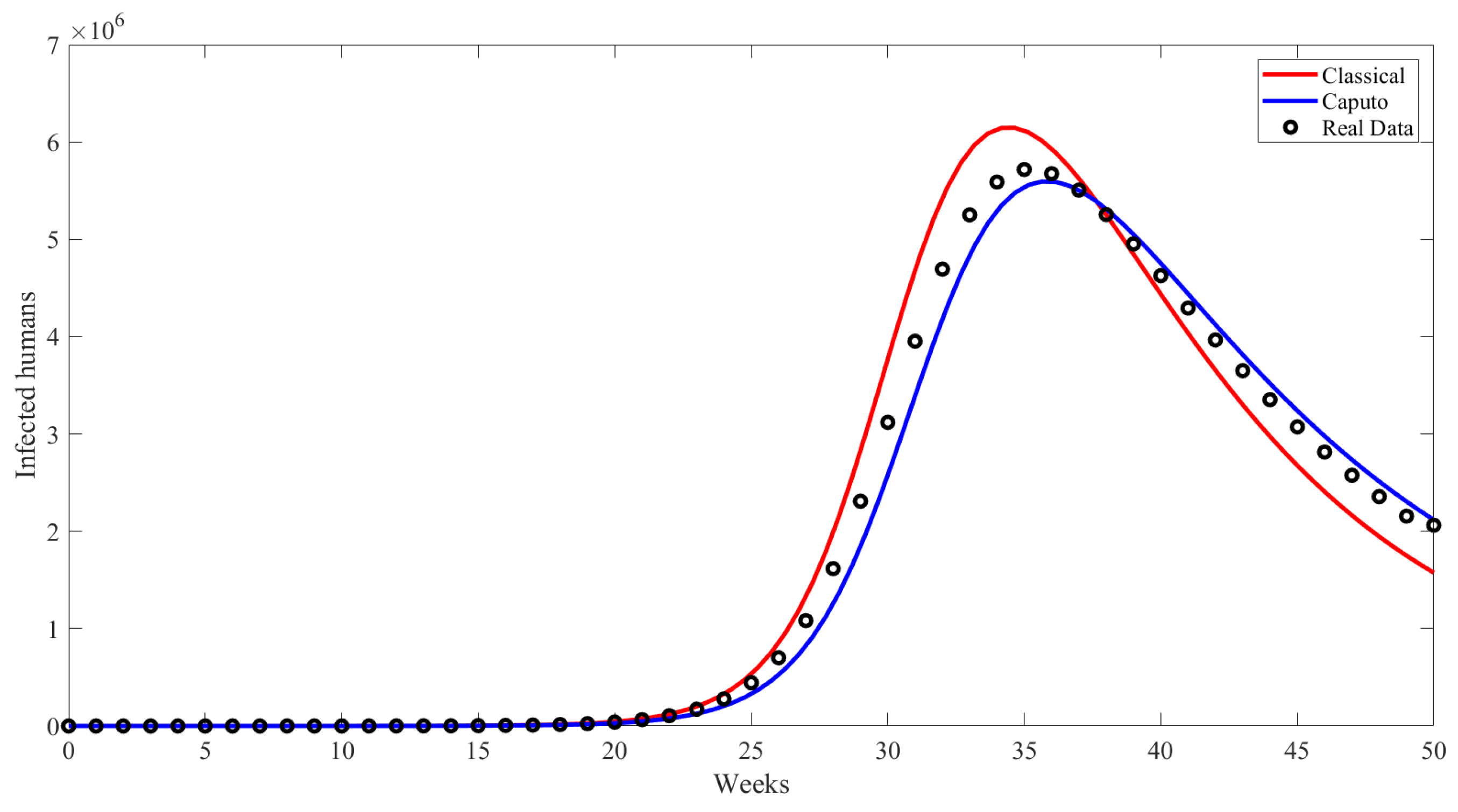
6. Numerical Results and Discussion

In this part, we present solutions for model (18) using Caputo, CF, and ABC.

$${}^{*}\mathcal{D}_{0,t}^{\alpha }u\left(t\right)=W\left(u\left(t\right)\right),t\in [0, a],u\left(0\right)=x_0,$$

(19)

where the symbol * represents a fractional operator. If we use (19), we get

$$u\left(t\right)=x_0+{}^{J_0^t}I^{\alpha }W\left(u\left(t\right)\right),t\in [0, a],$$

(20)

Let $u_r$ approximate $u\left(t\right)$ at $t=t_r$ for $r=0, 1, \dots , n$. $\Delta t(=0.05)={\displaystyle \frac{a}{n}},n\in \mathbb{N}$, over $[0, a]$; see [46].

$$C_{u_{r+1}}=u_0+{\displaystyle \frac{{(\Delta t)}^{\alpha }}{\Gamma (\omega +1)}}\sum _{T=0}^r{[r-T+1]}^{\omega }-{[r-T]}^{\omega }]W\left(u_T\right)+\mathcal{O}(\Delta t^2),$$

(21)

$$C{F}_{u_{r+1}}=u_0+(1-\delta )W\left(u_r\right)+\delta \Delta t\sum _{T=0}^{r}W\left(u_T\right)+\mathcal{O}(\Delta t^2),$$

(22)

$$AB{C}_{u_{r+1}}=u_0+{\displaystyle \frac{1-\alpha }{AB\left(\alpha \right)}}W\left(u_r\right)+{\displaystyle \frac{{(\Delta t)}^{\alpha }}{AB\left(\alpha \right)}}\sum _{T=0}^r{[r-T+1]}^{\alpha }-{[r-T]}^{\alpha }]W\left(u_T\right)+\mathcal{O}(\Delta t^2),$$

(23)

The visual comparisons display the weekly seasonal influenza cases collected from the Ministry of Health’s KSA [47]. In Figure 2, the accuracy of the classical model in forecasting the number of weekly seasonal influenza cases is demonstrated. The x-axis displays the number of weeks, while the y-axis depicts the number of infected people. The solid blue line represents the projections of the classical model, and the black circles indicate the actual data. The classical model satisfactorily approximates the data, accurately capturing seasonal influenza’s overall pattern and essential characteristics.

Figure 3 compares different values of the fractional order with accurate data in the Caputo model to determine the best fractional order for predicting weekly seasonal influenza cases. Figure 4 presents a detailed examination of fractional order values in the Caputo model, indicating that $0.99$ is the most effective fractional order for precise weekly seasonal influenza incidence prediction. This highlights the Caputo model’s superior performance in accurately matching the actual data, particularly in identifying infected individuals’ peaks and subsequent decreases.

Figure 5 compares different values of the fractional order in the Caputo–Fabrizio model to determine the best fractional order for predicting weekly seasonal influenza cases. The fractional orders of $0.96$ in the Caputo–Fabrizio model demonstrate the best performance in predicting weekly seasonal influenza cases, providing the closest fit to the real data.

Furthermore, in Figure 6, the performance of the Caputo–Fabrizio model in predicting weekly seasonal influenza cases is compared to the classical model and real data. The Caputo–Fabrizio model outperforms the classical model in predicting weekly seasonal influenza cases, bearing a closer resemblance to real data, particularly in capturing the peak and subsequent decline of infected individuals.

Figure 7 compares various fractional order values in the Atangana–Baleanu–Caputo (ABC) model to identify the most optimal fractional order for accurately forecasting weekly seasonal influenza cases. The study found that a fractional order of $0.95$ in the Atangana–Baleanu–Caputo model demonstrates superior predictive ability for weekly seasonal influenza cases. This value closely matches the actual data, particularly in accurately capturing infected persons’ peak and subsequent decline.

Additionally, in Figure 8, the performance of the Atangana–Baleanu–Caputo model in predicting weekly seasonal influenza cases is compared to the classical model and real data. The Atangana–Baleanu–Caputo model predicts weekly seasonal influenza cases better than the classical model, fitting the real data better, especially in capturing infected individuals’ peak and subsequent decline. A thorough evaluation of various fractional order values was performed by comparing them against actual data from weekly influenza cases to establish the most appropriate fractional order for each model. Afterward, the mean absolute value was computed for each fractional order value to choose the model with the lowest mean absolute value and was thus regarded as the most efficient. Figure 9, Figure 10, Figure 11, Figure 12 and Figure 13 shows simulation results for the susceptible, vaccinated, exposed, hospitalised, and recovered behaviors. Reapectively under the Caputo ($\alpha =0.99$), CF ($\alpha =0.96$), and ABC ($\alpha =0.95$),

Fractional models have been shown to reduce relative errors compared to classical models see Figure 14. These relative errors are found numerically to be $6.6e$, $5.8e$, and $1.2e$ for the Caputo ($\alpha =0.99$), the CF ($\alpha =0.96$), and the ABC ($\alpha =0.95$), respectively. Therefore, the classical approach is less effective compared to the fractional approach. The fractional model accounts for memory effects using non-local operators, such as fractional derivatives and integrals.

The root mean square error (RMSE) and mean absolute error (MAE) are two basic measures that can be employed to assess the performance of predictive models. An advantage of the RMSE is the fact that it is sensitive to significant errors because of the squared term used in its computation, making it suitable for problem domains where specific significant errors are not acceptable:

$$\mathrm{RMSE}=\sqrt{{\displaystyle \frac{1}{n}}\sum _{i=1}^n{(y_i-{\widehat{y}}_i)}^2}$$

(24)

where ${\widehat{y}}_i$ is the model-generated value and n is the number of observations. In contrast, MAE tells the average absolute value of errors for a set of predictions without regard to their direction and thus is one of the most straightforward measures of accuracy. It is defined as:

$$\mathrm{MAE}={\displaystyle \frac{1}{n}}\sum _{i=1}^n|y_i-{\widehat{y}}_i|$$

(25)

Both are useful in model assessment, but RMSE is more influenced by outliers, while MAE gives an overall average model assessment.

Table 3. MAE and RMSE for the Caputo operator for different fractional orders.

Fractional Order	MAE	RMSE
0.99	$1.004\times {10}^6$	$3.867\times {10}^6$
0.98	$1.103\times {10}^6$	$3.887\times {10}^6$
0.97	$1.690\times {10}^6$	$3.908\times {10}^6$
0.96	$1.102\times {10}^6$	$3.929\times {10}^6$
0.95	$1.136\times {10}^6$	$3.952\times {10}^6$

shows the calculated values of root mean square error (RMSE) and mean absolute error (MAE) for the Caputo operator at various fractional orders. The result of a more effective fractional order value was $\alpha$ = 0.95.

Table 4. MAE and RMSE for the Caputo–Fabrizio operator for different fractional orders.

Fractional Order	MAE	RMSE
0.99	$7.271\times {10}^5$	$3.753\times {10}^6$
0.98	$7.010\times {10}^5$	$3.756\times {10}^6$
0.97	$6.755\times {10}^5$	$3.760\times {10}^6$
0.96	$6.499\times {10}^5$	$3.725\times {10}^6$
0.95	$6.563\times {10}^5$	$3.771\times {10}^6$

shows the calculated values of root mean square error (RMSE) and mean absolute error (MAE) for the Caputo Fabrizio operator at various fractional orders. The result of a more effective fractional order value was $\alpha$ = 0.95.

Table 5. MAE and RMSE for the Atangana–Baleanu–Caputo operator for different fractional orders.

Fractional Order	MAE	RMSE
0.99	$6.068\times {10}^5$	$3.608\times {10}^6$
0.98	$5.912\times {10}^5$	$3.615\times {10}^6$
0.97	$5.796\times {10}^5$	$3.624\times {10}^6$
0.96	$5.787\times {10}^5$	$3.633\times {10}^6$
0.95	$5.531\times {10}^5$	$3.604\times {10}^6$
Classical	$6.475\times {10}^6$	$3.933\times {10}^6$

shows the calculated values of root mean square error (RMSE) and mean absolute error (MAE) for the Atangana–Baleanu–Caputo operator at various fractional orders. The result of a more effective fractional order value was $\alpha$ = 0.95. Further, the study’s findings show that ABC has been deemed the most superior of the three fractional order operators based on the lower error values.

7. Conclusions

This study compares the performance of fractional-order models ABC, CF, and Caputo with integer-order models. We used data from weekly influenza cases in KSA for 2022 to simulate integer-order and fractional-order models under the ABC, CF, and Caputo operators. Fractional-order models produced lower RMSE and MAE values than the integer-order model. The findings revealed that mathematical models with fractional orders outperform the integer-order model in forecasting influenza cases. In the Caputo–Fabrizio model, we found that 0.96 is the best fractional order for representing the dynamics of weekly seasonal influenza cases. The Caputo–Fabrizio model is better than the classical model at predicting weekly influenza cases, especially when showing infected individuals’ peaks and declines. Additionally, we found that 0.99 is the best fractional order for the Caputo model, and the Caputo model accurately predicts the number of people who will get influenza. Furthermore, we found that the best fractional order for Atangana–Baleanu–Caputo is 0.95, and the ABC model demonstrates superior predictive ability for weekly seasonal influenza cases. This value closely matches the data, particularly in accurately capturing infected persons’ peak and subsequent decline. Future work should explore fractional stochastic models’ effectiveness by integrating stochastic models and machine-learning algorithms for better prediction [40,48]. It will enhance the appreciation of the characteristics of diseases so that control measures can be enhanced.

References

1. Hutchinson, E.C. Influenza virus. Trends Microbiol. 2018, 26, 809–810. [Google Scholar] [CrossRef] [PubMed]
2. Al-Khuwaitir, T.S.; Al-Abdulkarim, A.S.; Abba, A.A.; Yousef, A.M.; El-Din, M.A.; Rahman, K.T.; Ali, M.A.; Mohamed, M.E.; Arnous, N.E. H1N1 influenza A. Preliminary evaluation in hospitalized patients in a secondary care facility in Saudi Arabia. Saudi Med. J. 2009, 30, 1532–1536. [Google Scholar]
3. Clark, N.M.; Lynch, J.P. Influenza: Epidemiology, clinical features, therapy, and prevention. Semin. Respir. Crit. Care Med. 2011, 32, 373–392. [Google Scholar] [CrossRef]
4. Javanian, M.; Barary, M.; Ghebrehewet, S.; Koppolu, V.; Vasigala, V.; Ebrahimpour, S. A brief review of influenza virus infection. J. Med. Virol. 2021, 93, 4638–4646. [Google Scholar] [CrossRef] [PubMed]
5. Sinha, R.; Paredis, C.J.; Liang, V.C.; Khosla, P.K. Modeling and simulation methods for design of engineering systems. J. Comput. Inf. Sci. Eng. 2001, 1, 84–91. [Google Scholar] [CrossRef]
6. Chinviriyasit, W. Numerical modeling of the transmission dynamics of influenza. In Proceedings of the First International Symposium on Optimization and Systems Biology, Beijing, China, 8–10 August 2007; pp. 52–59. [Google Scholar]
7. Casagrandi, R.; Bolzoni, L.; Levin, S.A.; Andreasen, V. The SIRC model and influenza A. Math. Biosci. 2006, 200, 152–169. [Google Scholar] [CrossRef]
8. Anderson, R.M.; May, R.M. Infectious Diseases of Humans: Dynamics and Control; Oxford University Press: Oxford, UK, 1991. [Google Scholar]
9. Elbasha, E.H.; Podder, C.N.; Gumel, A.B. Analyzing the dynamics of an SIRS vaccination model with waning natural and vaccine-induced immunity. Nonlinear Anal. Real World Appl. 2011, 12, 2692–2705. [Google Scholar] [CrossRef]
10. Iwami, S.; Takeuchi, Y.; Liu, X. Avian–human influenza epidemic model. Math. Biosci. 2007, 207, 1–25. [Google Scholar] [CrossRef]
11. Jung, E.; Iwami, S.; Takeuchi, Y.; Jo, T.C. Optimal control strategy for prevention of avian influenza pandemic. J. Theor. Biol. 2009, 260, 220–229. [Google Scholar] [CrossRef]
12. Lucchetti, J.; Roy, M.; Martcheva, M. An avian influenza model and its fit to human avian influenza cases. Adv. Dis. Epidemiol. 2009, 1, 1–30. [Google Scholar]
13. Iwami, S.; Takeuchi, Y.; Liu, X.; Nakaoka, S. A geographical spread of vaccine-resistance in avian influenza epidemics. J. Theor. Biol. 2009, 259, 219–228. [Google Scholar] [CrossRef] [PubMed]
14. Ruan, S.; Wang, W. Dynamical behavior of an epidemic model with a nonlinear incidence rate. J. Differ. Equations 2003, 188, 135–163. [Google Scholar] [CrossRef]
15. Khader, M.M.; Sweilam, N.H.; Mahdy, A.M.S.; Moniem, N.K. Numerical simulation for the fractional SIRC model and influenza A. Appl. Math. Inf. Sci. 2014, 8, 1029. [Google Scholar] [CrossRef]
16. Alsubaie, N.E.; EL Guma, F.; Boulehmi, K.; Al-kuleab, N.; Abdoon, M.A. Improving Influenza Epidemiological Models under Caputo Fractional-Order Calculus. Symmetry 2024, 16, 929. [Google Scholar] [CrossRef]
17. Al-Qureshi, M.; Rashid, S.; Jarad, F.; Alharthi, M.S. Dynamical behavior of a stochastic highly pathogenic avian influenza A (HPAI) epidemic model via piecewise fractional differential technique. AIMS Math. 2023, 8, 1737–1756. [Google Scholar] [CrossRef]
18. Alharbi, S.A.; Abdoon, M.A.; Saadeh, R.; Alsemiry, R.D.; Allogmany, R.; Berir, M.; EL Guma, F. Modeling and analysis of visceral leishmaniasis dynamics using fractional-order operators: A comparative study. Math. Methods Appl. Sci. 2024, 47, 9918–9937. [Google Scholar] [CrossRef]
19. Algahtani, O.J.J. Comparing the Atangana–Baleanu and Caputo–Fabrizio derivative with fractional order: Allen Cahn model. Chaos Solitons Fractals 2016, 89, 552–559. [Google Scholar] [CrossRef]
20. Atangana, A.; Owolabi, K.M. New numerical approach for fractional differential equations. Math. Model. Nat. Phenom. 2018, 13, 3. [Google Scholar] [CrossRef]
21. Alkahtani, B.S.T. Chua’s circuit model with Atangana–Baleanu derivative with fractional order. Chaos Solitons Fractals 2016, 89, 547–551. [Google Scholar] [CrossRef]
22. Yavuz, M.; Özdemir, N. European vanilla option pricing model of fractional order without singular kernel. Fractal Fract. 2018, 2, 3. [Google Scholar] [CrossRef]
23. Abdoon, M.A.; Saadeh, R.; Berir, M.; Guma, F.E. Analysis, modeling and simulation of a fractional-order influenza model. Alex. Eng. J. 2023, 74, 231–240. [Google Scholar] [CrossRef]
24. Alzahrani, S.M.; Saadeh, R.; Abdoon, M.A.; Qazza, A.; Guma, F.E.; Berir, M. Numerical Simulation of an Influenza Epidemic: Prediction with Fractional SEIR and the ARIMA Model. Appl. Math. 2024, 18, 1–12. [Google Scholar]
25. Saadeh, R.; Abdoon, M.A.; Qazza, A.; Berir, M. A numerical solution of generalized Caputo fractional initial value problems. Fractal Fract. 2023, 7, 332. [Google Scholar] [CrossRef]
26. Elbadri, M.; Abdoon, M.A.; Berir, M.; Almutairi, D.K. A symmetry chaotic model with fractional derivative order via two different methods. Symmetry 2023, 15, 1151. [Google Scholar] [CrossRef]
27. Alzahrani, A.B.; Abdoon, M.A.; Elbadri, M.; Berir, M.; Elgezouli, D.E. A comparative numerical study of the symmetry chaotic jerk system with a hyperbolic sine function via two different methods. Symmetry 2023, 15, 1991. [Google Scholar] [CrossRef]
28. Khan, H.; Rajpar, A.H.; Alzabut, J.; Aslam, M.; Etemad, S.; Rezapour, S. On a Fractal–Fractional-Based Modeling for Influenza and Its Analytical Results. Qual. Theory Dyn. Syst. 2024, 23, 70. [Google Scholar] [CrossRef]
29. Huang, J.; Cen, Z.; Xu, A.; He, T.; Liu, Q. A Fractional SIR Model for the Simulation of the Spread of Influenza A during the Post COVID-19 Period. Available online: https://papers.ssrn.com/sol3/papers.cfm?abstract_id=4786433 (accessed on 8 April 2024).
30. Andreu-Vilarroig, C.; Villanueva, R.J.; González-Parra, G. Mathematical modeling for estimating influenza vaccine efficacy: A case study of the Valencian Community, Spain. Infect. Dis. Model. 2024, 9, 744–762. [Google Scholar] [CrossRef]
31. Zhang, L.; Ma, C.; Duan, W.; Yuan, J.; Wu, S.; Sun, Y.; Zhang, J.; Liu, J.; Wang, Q.; Liu, M. The role of absolute humidity in influenza transmission in Beijing, China: Risk assessment and attributable fraction identification. Int. J. Environ. Health Res. 2024, 34, 767–778. [Google Scholar] [CrossRef]
32. Zhang, X.; Zhang, X. Dynamical Behavior and Numerical Simulation of an Influenza A Epidemic Model with Log-Normal Ornstein–Uhlenbeck Process. Qual. Theory Dyn. Syst. 2024, 23, 190. [Google Scholar] [CrossRef]
33. Alshareef, A. Quantitative analysis of a fractional order of the SEIcIηVR epidemic model with vaccination strategy. AIMS Math. 2024, 9, 6878–6903. [Google Scholar] [CrossRef]
34. Yavuz, M.; Arfan, M.; Sami, A. Theoretical and numerical investigation of a modified ABC fractional operator for the spread of polio under the effect of vaccination. AIMS Biophys. 2024, 11, 97–120. [Google Scholar]
35. Podlubny, I. Fractional Differential Equations: An Introduction to Fractional Derivatives, Fractional Differential Equations, to Methods of Their Solution and Some of Their Applications; Elsevier: Amsterdam, The Netherlands, 1998. [Google Scholar]
36. Caputo, M.; Fabrizio, M. A new definition of fractional derivative without singular kernel. Prog. Fract. Differ. Appl. 2015, 1, 73–85. [Google Scholar]
37. Atangana, A.; Baleanu, D. New fractional derivatives with nonlocal and non-singular kernel: Theory and application to heat transfer model. arXiv 2016, arXiv:1602.03408. [Google Scholar] [CrossRef]
38. Malomed, B.A. Fractional wave models and their experimental applications. In Fractional Dispersive Models and Applications: Recent Developments and Future Perspectives; Springer: Berlin/Heidelberg, Germany, 2024; pp. 1–30. [Google Scholar]
39. Macrotrends: Saudi Arabia Population 1950–2023. 2021–2022. Available online: https://www.macrotrends.net/countries/SAU/saudi-arabia/population (accessed on 3 August 2024).
40. Cori, A.; Valleron, A.J.; Carrat, F.; Tomba, G.S.; Thomas, G.; Boëlle, P.Y. Estimating influenza latency and infectious period durations using viral excretion data. Epidemics 2012, 4, 132–138. [Google Scholar] [CrossRef]
41. Takele, R. Stochastic modelling for predicting COVID-19 prevalence in East Africa Countries. Infect. Dis. Model. 2020, 5, 598–607. [Google Scholar] [CrossRef]
42. Ahmad, J.; Ali, F.; Murtaza, S.; Khan, I. Caputo time fractional model based on generalized Fourier’s and Fick’s laws for Jeffrey nanofluid: Applications in automobiles. Math. Probl. Eng. 2021, 2021, 4611656. [Google Scholar] [CrossRef]
43. Kumar, S.; Shaw, P.K.; Abdel-Aty, A.H.; Mahmoud, E.E. A numerical study on fractional differential equation with population growth model. Numer. Methods Partial. Differ. Equations 2024, 40, e22684. [Google Scholar] [CrossRef]
44. Khan, F.M.; Khan, Z.U. Numerical analysis of fractional order drinking mathematical model. J. Math. Tech. Model. 2024, 1, 11–24. [Google Scholar]
45. Van den Driessche, P.; Watmough, J. Reproduction numbers and sub-threshold endemic equilibria for compartmental models of disease transmission. Math. Biosci. 2002, 180, 29–48. [Google Scholar] [CrossRef]
46. Qureshi, S.; Atangana, A. Mathematical analysis of dengue fever outbreak by novel fractional operators with field data. Phys. A Stat. Mech. Its Appl. 2019, 526, 121127. [Google Scholar] [CrossRef]
47. Statista. Saudi Arabia: Life Expectancy at Birth from 2011 to 2021. Available online: https://www.statista.com/statistics/262477/life-expectancy-at-birth-in-saudi-arabia/ (accessed on 27 May 2024).
48. Mao, Y.; Yu, X. A hybrid forecasting approach for China’s national carbon emission allowance prices with balanced accuracy and interpretability. J. Environ. Manag. 2024, 351, 119873. [Google Scholar] [CrossRef]
Figure 1. Influenza transmission dynamics.
Symmetry 16 01126 g001
Figure 2. Comparing the classical model for infected people with real data.
Symmetry 16 01126 g002
Figure 3. Comparing the Caputo model for infected people with real data.
Symmetry 16 01126 g003
Figure 4. Comparing classical model and Caputo model for infected people with real data.
Symmetry 16 01126 g004
Figure 5. Comparing the CF model for infected people with real data.
Symmetry 16 01126 g005
Figure 6. Comparing classical model and CF model for infected people with real data.
Symmetry 16 01126 g006
Figure 7. Comparing the ABC model for infected people with real data.
Symmetry 16 01126 g007
Figure 8. Comparing classical model and ABC model for infected people with real data.
Symmetry 16 01126 g008
Figure 9. Simulation results for susceptible behavior under different operators.
Symmetry 16 01126 g009
Figure 10. Simulation results for vaccinated behavior under different operators.
Symmetry 16 01126 g010
Figure 11. Simulation results for exposed behavior under different operators.
Symmetry 16 01126 g011
Figure 12. Simulation results for hospitalized behavior under different operators.
Symmetry 16 01126 g012
Figure 13. Simulation results for recovered behavior under different operators.
Symmetry 16 01126 g013
Figure 14. Comparing classical model and Caputo, CF, and ABC models for infected people with real data.
Symmetry 16 01126 g014