Abstract
In many manufacturing industries, the lifetime performance index is utilized to assess the manufacturing process performance for products following some lifetime distributions and subjecting them to progressive type I interval censoring. This paper aims to explore the sampling design required to achieve a specified level of significance and test power for products with lifetimes following the Exponentiated Frech’et distribution. Since lifetime distribution is an asymmetrical probability distribution, this investigation is related to the topic of asymmetrical probability distributions and applications in various fields. When the termination time is fixed but the number of intervals is variable, the optimal number of inspection intervals and sample sizes yielding the minimized total experimental costs are determined and tabulated. When the termination time is varying, the optimal number of inspection intervals, sample sizes, and equal interval lengths achieving the minimum total experimental costs are determined and tabulated. Optimal parameter values are displayed in tabular form for feasible applications for users. Additionally, a practical example is provided to illustrate how this sampling design can be used to collect data by using the optimal setup of parameters, followed by a testing procedure to assess the capability of the production process.
1. Introduction
To assess ‘the-larger-the-better’ quality characteristics, such as lifespan, fuel efficiency in vehicles, and heat resistance, the lifetime performance index Montgomery [1] is frequently employed. This index is defined as where μ is regarded as the process mean, σ is regarded as the process standard deviation and L is the specified lower specification limit. Tong et al. [2] developed a hypothesis testing procedure for when products have lifetimes following an exponential distribution using the uniformly minimum variance unbiased estimator as the test statistic based on the complete sample. However, there are numerous cases where experimenters cannot observe the lifetimes of all items due to budget restrictions, time limitations and other factors. This leads to censoring. For progressive censoring, some detailed insights into the analysis and application of progressive censored data can be seen by referring to Cohen [3], Balakrishnan [4], Balakrishnan and Aggarwala [5], Gupta [6], Chen and Zhang [7] and Wang and Liu [8]. For progressive type I interval censored data, Wu and Lin [9] proposed a testing procedure for the lifetime performance index for exponential products using the maximum likelihood estimator as the test statistic. Wu et al. [10] developed a hypothesis testing procedure for the evaluation of this index for products with Burr XII distribution. Wu [11] proposed a testing procedure for products with lifetimes following the Exponentiated Frech’et distribution based on a progressive type I interval censored sample. The testing procedure for this index is synopsized in Section 2. To our best knowledge, there is no research related to finding the optimal experimental design for this testing procedure for products’ lifetimes following the Exponentiated Frech’et distribution. To fill in this research gap, the contribution and novelty of this investigation is that it finds the optimal experimental design for the level test related to the lifetime performance index when the termination time for an experiment on progressive type I interval censoring is fixed or varying.
The paper is structured as follows: We determine the minimum sample size required to reach the pre-specified significance level and test power in Section 2. When the termination time for the experiment is fixed, we investigate the sampling design, aiming to minimize the total experimental costs under a specific cost structure in Section 3.1. When the termination time for the experiment is varying, we find an optimal sampling design yielding minimized total experimental costs in Section 3.2. With the aim of illustrating how to apply our optimal experimental design, one practical example is provided in Section 3.3. Finally, the findings and conclusion are summarized in Section 4.
2. Introduction to the Testing Procedure for the Lifetime Performance Index and Minimum Sample Size
We assume that the lifetime U of products follows an Exponentiated Frech’et distribution with the probability density function (pdf), the cumulative distribution function (cdf) and the hazard function as follows:
The Exponentiated Frech’et distribution has a hazard function with a mono peak shape, and it is an asymmetrical probability distribution. This study is related to the topic of asymmetrical probability distributions and applications across disciplines. This distribution is commonly employed to characterize human mortality. Through the variable transformation , we yield a new random variable Y with a one-parameter exponential distribution, and its pdf, cdf and hazard function are given in Equations (4)–(6) as follows:
If the users specify the lower specification limit for U to be LU, then we can find the corresponding lower specification limit for Y to be .
The mean and standard deviation of Y are = 1/ and = 1/. By substituting = 1/ and = 1/ into , the lifetime performance index .
The yield rate is obtained as
Evidently, the yield rate increases with .
The progressive type I interval censoring scheme is depicted as follows: We begin the lifetime test of n products at time 0. Let (t1, …, tm) be the predetermined inspection time points and (p1, …, pm) be the removal probabilities for the progressive censoring at times (t1, …, tm), where pm = 1 and tm = T is the termination time of the experiment. At the ith inspection time point ti, the number of failure units Xi is observed, which is following a binomial distribution bin(,qi), where and FU(x) denotes the cdf for the lifetime variable U, and it is defined in Equation (2). At this time point, we remove Ri units randomly from the remaining survival units and Ri follows a binomial distribution bin(,pi), i = 1, …, m. At the end of the experiment, we collect the progressive type I interval censored sample (X1, …, Xm) under the progressive censoring scheme of (R1, …, Rm) with removal probabilities p1, …, pm. Based on this censored sample, Wu [11] derived the maximum likelihood estimator of denoted as by solving the log-likelihood equation, given as follows:
Fisher’s information number is found to be
By the property of maximum likelihood estimator (MLE), we can find the approximate normal distribution of , i.e., .
Consider the case of equal interval lengths, i.e., Replacing = it, in Equations (7) and (8), we can find the simpler form of MLE and Fisher’s information number.
Based on the invariance property of MLE, the MLE of can be found as
Likewise, we can find the approximate normal distribution of .
If the analysts set to be the desired target level for the lifetime performance index to make the process capable, we want to test (the process is not capable) vs. (the process is capable). Under the level of significance , we use the MLE of as the test statistic. The rejection region is determined as R = {, where , and denotes the percentile of standard normal distribution.
In the alternative hypothesis, we consider the point of and define as the deviation of the true parameter value from the target level . The power h() is obtained as
where is the cdf of a standard normal distribution, and
Let = =, which is not a function of the sample size n. For a level test with the given type II error probability at , we set the test power to be as . Solving this equation, we obtain the required minimum sample size as
where ceil (.) is the smallest integer greater than or equal to a given number.
3. Reliability Sampling Design
The reliability sampling design is crucial for analysts planning a progressive type I interval censoring experiment. In Section 3.1, with a fixed total experimental time T, we determine the required sample size and minimal number of inspection intervals to reach the given test power of the level test and minimize the total experimental costs. In Section 3.2, with a varying total experimental time T, we determine the minimal number of inspection intervals, the corresponding equal length of interval and the required sample size to minimize the total experimental costs. In Section 3.3, we give an example for the aim of illustration.
3.1. The Determination of the Optimal m and n When the Termination Time T Is Fixed
Analysts typically prefer to not to have a large number of inspection intervals, denoted as m, which needs to be determined in this section. Users can assign the value of m0 as the upper limit of m such that (the defaulted number of m0 is 20). Once the optimal number of m is determined, we can determine the related sample size n by using Equation (11). The cost structure we consider is similar to that used by Huang and Wu [12], and it is composed of the following four costs:
- Inspection cost CI: the cost of using the inspection equipment for each inspection;
- Sample cost Cs: the cost for one test unit in the sample;
- Operation cost Co: the cost per unit of time, encompassing expenses like personnel costs and the depreciation of test equipment;
- Installation cost Ca: the fixed cost for installing all test units.
Incorporating all costs, we yield the total cost of
We employ a enumerative method to find the optimal (m,n) denoted by (m*,n*). The optimal (m*,n*) yielding the minimized total experimental cost is determined and tabulated.
The determination of the optimal (m*,n*) is outlined in the following seven steps:
- Step 1: Provide the predetermined values of c0, c1, , , , T, L, and the costs of CI = a Ca, Cs = b Ca, Co = c Ca.
- Step 2: Compute and
- Step 3: Set m = 1.
- Step 4: Calculate the sample size n using Equation (11), followed by determining the associated total cost TC(m,n) by the use of Equation (12).
- Step 5: If , then m = m + 1 and go to Step 4; otherwise, go to Step 6.
- Step 6: The optimal value of m denoted by m* is found to be the minimum value of m such that TC* = TC(m,n) is attained and the related sample size n* can be obtained by using Equation (11).
- Step 7: The critical value in the critical region can be calculated as .
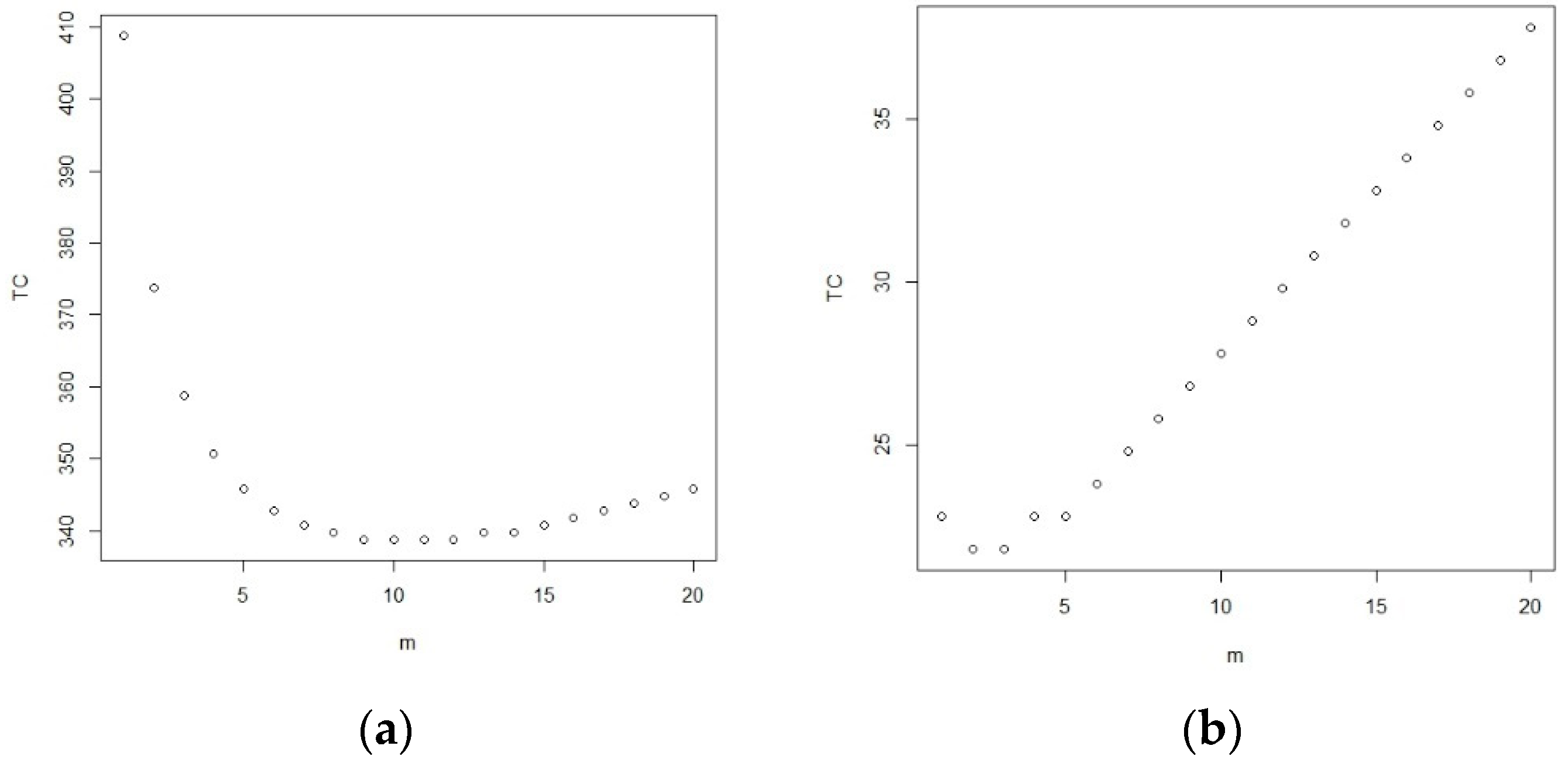
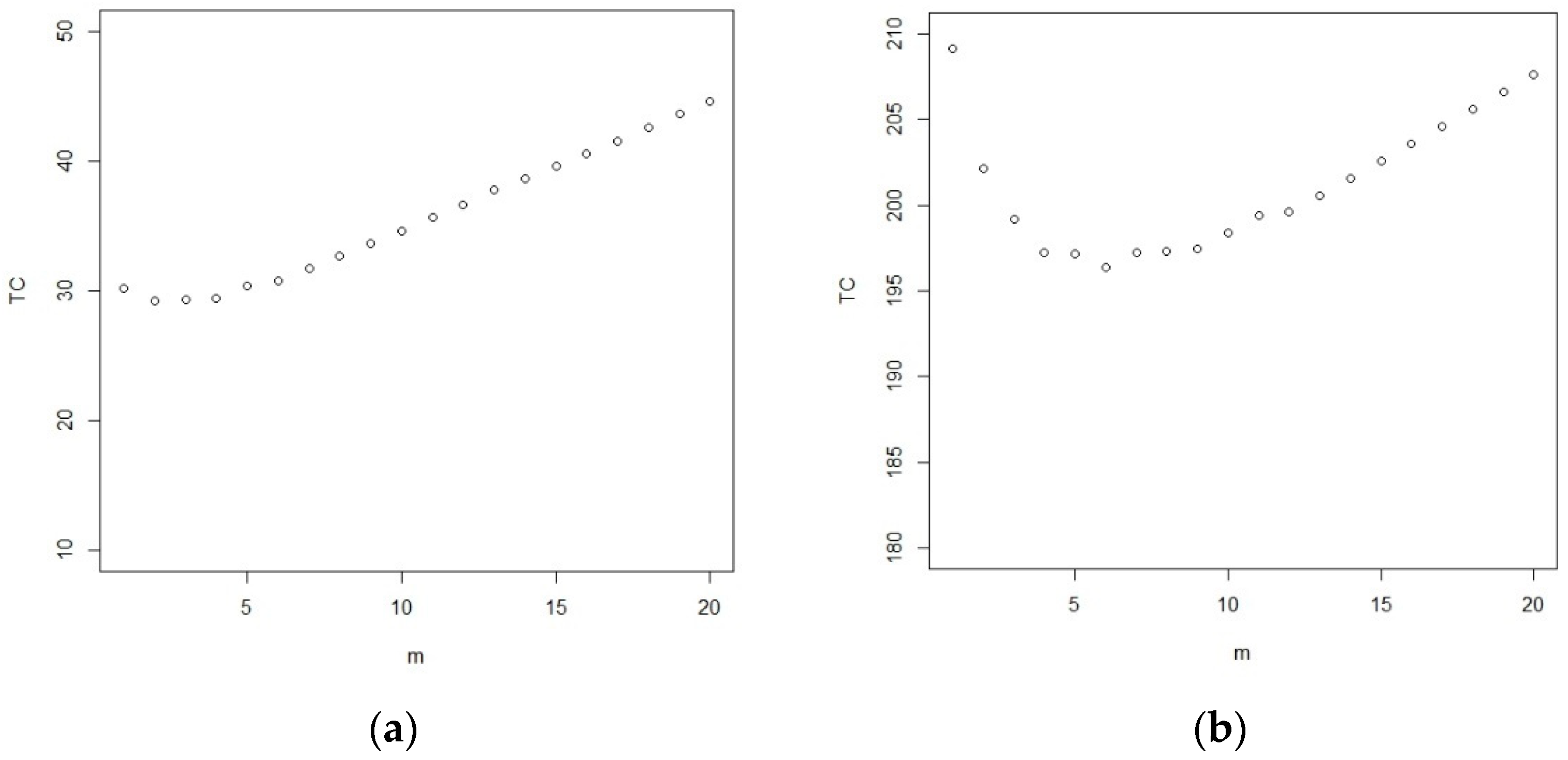
We consider the cost structure of Ca = 1 and a = b = c = 1. To test when = 0.15, , p = 0.05, c1 = 0.80, L = 0.05, T = 0.8, we graph the total cost against m = 1, …, m0 in Figure 1a. The minimum total cost of 338.8 is observed from this figure when m = 9. For the other setup of parameters = 0.1, = 0.1, p = 0.05, c1 = 0.875, L = 0.05, T = 0.8, we graph the total cost against m = 1, …, m0 in Figure 1b. The curve exhibits a concave upward shape with intermittent flat sections, and we can find that the minimum total cost of 21.8 is observed from this figure when m = 2.
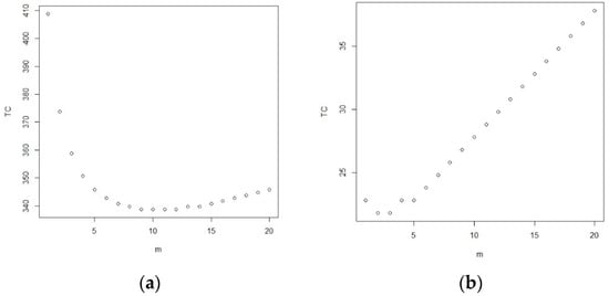
Figure 1.
(a): The curve of total cost at = 0.15, , p = 0.05, c1 = 0.80. (b) The curve of total cost at = 0.1, = 0.1, p = 0.05, c1 = 0.875.
The optimal inspection intervals m* and the related sample size n* are determined to yield the minimum total cost TC(m*,n*) for testing , and the optimal m* and n* are tabulated in Table A1 and Table A2 of the Appendix A section at , , and L = 0.05, for and , respectively. The corresponding critical values are also tabulated.
For instance, if the analyst seeks to perform a hypothesis test at a significance level of 0.01, with a power of 0.8, under the conditions = 0.80, p = 0.05 and m0 = 20, we can find the required minimum sample size to be 188 with six inspection intervals from Table A1. This table also shows that the minimum total cost is TC = 195.8 with the critical value of 0.7778.
From Table A1 and Table A2, we observe that (1) as increases across various combinations of , and p, the required minimum sample size is decreasing; (2) the required minimum sample size increases as the significance level decreases, across all combinations of and p; (3) the required minimum sample size is an increasing function of the probability of type II error ; (4) the minimum number of inspection intervals decreases as increases across all combinations of , and p; (5) the minimum number of inspection intervals is non-increasing as the type II error increases or the power 1 − ; (6) the minimum total cost decreases as increases across all combinations of , and p; (7) the minimum total cost is an increasing function of the removal probability p when , and are fixed; (8) the minimum total cost is a decreasing function of the test power 1 − .
3.2. The Determination of the Optimal m, t and n When the Termination Time T Is Varying
In this section, we examine scenarios where the inspection time t for each interval is varying. The goal is to identify the optimal (m,t,n) configuration that minimizes the total cost incurred during the type I interval censoring procedure. Using the same cost structure, the total cost can be written as
We employ a enumerative method to find the optimal (m,t,n) denoted by (m*,t*,n*).
The determination of the optimal (m*,t*,n*) is outlined in the following seven steps:
- Step 1: Provide the predetermined values of c0, c1, , , , L, and the costs of CI = a Ca, Cs = b Ca, Co = c Ca.
- Step 2: Compute and
- Step 3: Set m = 1.
- Step 4: The optimal value of t* is determined to minimize the total cost TC(m,t,n) given in Equation (13). Calculate the sample size n using Equation (11) and then compute the related total cost TC(m,t*,n) by using Equation (13).
- Step 5: If , then m = m + 1 and go to Step 4; otherwise, go to Step 6.
- Step 6: We determine the optimal choice of m denoted by m* as the minimum value of m such that TC** = TC(m,t*,n) is reached and then the corresponding sample size n* is determined by using Equation (11).
- Step 7: The critical value can be calculated as .
We consider the cost structure of Ca = 1 and a = b = c = 1. For testing , = 0.20, , p = 0.05, c1 = 0.875 and L = 0.05. In Figure 2a, we depict the plot of m = 1, …, m0 against its respective total cost. From this figure, it is shown that the total cost reaches its minimum of 29.248 when m = 2. Figure 2b displays an alternative total cost curve for different parameter settings: = 0.10, = 0.1, p = 0.1, c1 = 0.8 and L = 0.05 for m = 1, …, 20. The curve is concave upwards, and the minimum total cost of 196.331 is achieved at m = 6. We observe similar patterns with other combinations of setups.
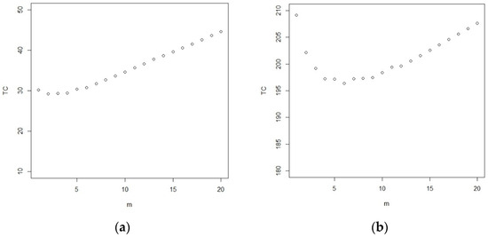
Figure 2.
(a): The curve of total cost at = 0.20, , p = 0.05, c1 = 0.875. (b) The curve of total cost at = 0.10, = 0.1, p = 0.1, c1 = 0.8.
For testing , we determine the optimal inspection intervals m*, inspection interval duration t* and sample size n* to yield the minimum total cost, and they are tabulated in Table A3 and Table A4 of the Appendix A section at , and L = 0.05, for and , respectively. We also tabulate the corresponding critical values .
For instance, consider if an analyst seeks to perform a hypothesis test at a significance level of 0.05, with a power of 0.8, under the conditions = 0.80, p = 0.05 and m0 = 20. According to Table A3, the required minimum sample size is determined as 249 with seven inspection intervals and an inspection interval time of 0.04. Under this setup, we yield the minimum total cost of TC = 257.3 with the critical value of 0.7809.
From Table A3 and Table A4, we observe that (1) the required minimum sample size increases as decreases across various combinations of , and p; (2) the required minimum sample size increases as the significance level decreases across all combinations of and p; (3) the required minimum sample size is a decreasing function of the power 1−; (4) the minimum number of inspection intervals decreases when increases across all combinations of , and p; (5) the minimum number of inspection intervals is non-increasing as the type II error increases or the power ; (6) the minimum total cost decreases when is increasing with , and p held constant; (7) the minimum total cost decreases or remains constant as the removal probability p increases, with , and held constant; (8) the minimum total cost is non-increasing as the test power 1 − .
3.3. Example
To assist users in applying our proposed hypothesis testing procedure to practical scenarios, we illustrate it with a specific numerical example. We analyze the relief times (in hours) U(1) … U(50) for 50 arthritic patients from Wingo [13] as follows: 0.29, 0.29, 0.34, 0.34, 0.35, 0.36, 0.36, 0.36, 0.44, 0.44, 0.46, 0.46, 0.49, 0.49, 0.50, 0.50, 0.52, 0.54, 0.55, 0.55, 0.55, 0.56, 0.57, 0.58, 0.59, 0.59, 0.60, 0.60, 0.61, 0.61, 0.62, 0.64, 0.68, 0.70, 0.70, 0.71, 0.71, 0.71, 0.72, 0.73, 0.75, 0.75, 0.80, 0.80, 0.81, 0.82, 0.84, 0.84, 0.84 and 0.87.
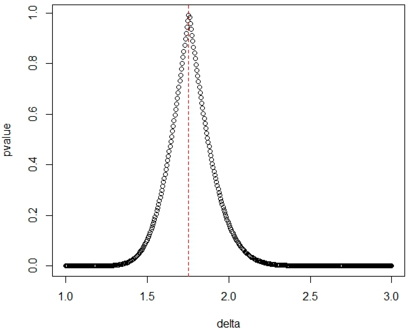
The Gini-test described by Gail and Gastwirth [14] is used to test the good fit of the Exponentiated Frechét distribution. The Gini-test value is defined as where , j = 1, …, 50. The Gini-test value is a function of , and the p-values versus values are displayed in Figure 3. The value of is determined with the the maximum p-value. From Figure 3, it is observed that the maximum p-value of 0.9926 occurs at .
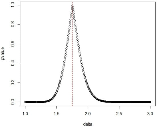
Figure 3.
The p-values versus the values of .
Regarding Section 3.1, we find the optimal number of inspection intervals to be m* = 2 and the required sample size to be n* = 36 from Table A2 under the consideration of = 0.01, the power 1 − = 0.80, p = 0.05 and the target lifetime performance index = 0.75 at the point of = 0.9 in the alternative hypothesis. With this setup, we yield the minimum total cost of 39.8 units under the cost setup of Co = 1 and a = b = c= 1.
Based on this optimal setup, we can proceed to perform the testing procedure for as follows:
- Step 1: Take a random sample 36 in size with m* = 2 from the data set. Collect the progressive type I interval censored sample (7, 24) at the pre-set times (0.4, 0.8) with censoring schemes of 0, 5).
- Step 2: Calculate the maximum likelihood estimator for as = 8.9934. We can find the maximum likelihood estimator for c as = 1 − 8.9934 (0.00255) = 0.9907.
- Step 3: For the level of = 0.01 test, the critical value is found to be = 0.8707.
- Step 4: Since 0.9907 > = 0.8707, we can infer that the null hypothesis should be rejected and conclude that the lifetime performance index attains the required target level c0, and we claim that the production process is capable.
Regarding Section 3.2, we find the optimal number of inspection intervals m* = 3, the optimal time length of each interval t* = 0.15, the required minimum sample size n* = 43 from Table A4 under the consideration of = 0.01, the power 1 − = 0.90, the removal probability p = 0.10 and the target lifetime performance index = 0.75 at = 0.875 in the alternative hypothesis. With this setup, we yield the minimum total cost of 47.5 units under the cost setup of Co = 1 and a = b = c = 1.
Based on this optimal setup, we can proceed to perform the testing procedure for as follows:
- Step 1: Take a random sample 43 in size from the data set. Observe the progressive type I interval censored sample = (0, 2, 4) at the pre-set times = (0.15, 0.30, 0.45) with censoring schemes of = (5, 4, 28).
- Step 2: Calculate the maximum likelihood estimator for as = 13.3962. Then, we can find the maximum likelihood estimator for as = 1 − 13.3962 (0.00255) = 0.9658.
- Step 3: For the level of the = 0.01 test, the critical value is found to be 0.8541.
- Step 4: Since 0.9658 > 0.8541, we arrive at the same conclusion to substantiate the alternative hypothesis.
4. Conclusions
In many practical scenarios, obtaining a complete sample can be prohibitively expensive. This necessitates the use of progressive type I interval censoring. Under this censoring scheme, we obtain the required sample size for a level α test related to the lifetime performance index for products following the Exponentiated Frechét distribution in order to achieve a specified test power. Additionally, we determine the minimum required sample size and number of inspection intervals when the experiment’s termination time is fixed, aiming to achieve the desired power and minimize the total experimental costs for a level α test. When the experiment’s termination time is varying, we establish the minimum required sample size, number of inspection intervals, and inspection interval length to achieve the specified test power and minimize the total experimental costs for a level α test under progressive type I interval censoring. To guide users, we provide a numerical example to illustrate how to determine the optimal setup for the experiment, followed by a testing procedure to evaluate whether the production process meets capability requirements. In the future, we will work on a new lifetime performance index by replacing the mean in CL by the median to better address the asymmetric distributions. A different censoring scheme like hybrid censoring can also be considered for the future research.
Funding
This research and the APC were funded by the National Science and Technology Council, Taiwan, NSTC 113-2118-M-032-002.
Data Availability Statement
Data are available in a publicly accessible repository. The data presented in this study are openly available in Wingo [13].
Conflicts of Interest
The author declares no conflicts of interest.
Appendix A

Table A1.
The optimal (m*,n*), total cost TC and critical value for and under , L = 0.05, T = 0.8 and .
Table A1.
The optimal (m*,n*), total cost TC and critical value for and under , L = 0.05, T = 0.8 and .
| 0.025 | 0.05 | |||||||||
|---|---|---|---|---|---|---|---|---|---|---|
| p | ||||||||||
| 0.01 | 0.20 | 0.050 | 20 | 1629 | 1650.8 | 0.7667 | 11 | 386 | 398.8 | 0.7847 |
| 0.075 | 18 | 1654 | 1673.8 | 0.7667 | 10 | 391 | 402.8 | 0.7847 | ||
| 0.100 | 17 | 1673 | 1691.8 | 0.7667 | 9 | 395 | 405.8 | 0.7847 | ||
| 0.15 | 0.050 | 15 | 1371 | 1387.8 | 0.7678 | 9 | 328 | 338.8 | 0.7867 | |
| 0.075 | 12 | 1398 | 1411.8 | 0.7678 | 8 | 333 | 342.8 | 0.7867 | ||
| 0.100 | 10 | 1419 | 1430.8 | 0.7678 | 8 | 336 | 345.8 | 0.7867 | ||
| 0.10 | 0.050 | 10 | 1202 | 1213.8 | 0.7688 | 8 | 288 | 297.8 | 0.7886 | |
| 0.075 | 9 | 1224 | 1234.8 | 0.7688 | 7 | 293 | 301.8 | 0.7886 | ||
| 0.100 | 8 | 1243 | 1252.8 | 0.7688 | 6 | 298 | 305.8 | 0.7886 | ||
| 0.05 | 0.20 | 0.050 | 18 | 1056 | 1075.8 | 0.7647 | 9 | 247 | 257.8 | 0.7808 |
| 0.075 | 16 | 1072 | 1089.8 | 0.7647 | 8 | 250 | 259.8 | 0.7808 | ||
| 0.100 | 15 | 1084 | 1100.8 | 0.7647 | 7 | 253 | 261.8 | 0.7808 | ||
| 0.15 | 0.050 | 13 | 861 | 875.8 | 0.7659 | 8 | 203 | 212.8 | 0.7831 | |
| 0.075 | 11 | 877 | 889.8 | 0.7659 | 7 | 206 | 214.8 | 0.7831 | ||
| 0.100 | 9 | 890 | 900.8 | 0.7659 | 6 | 209 | 216.8 | 0.7831 | ||
| 0.10 | 0.050 | 9 | 732 | 742.8 | 0.7671 | 6 | 175 | 182.8 | 0.7852 | |
| 0.075 | 8 | 745 | 754.8 | 0.7671 | 5 | 178 | 184.8 | 0.7853 | ||
| 0.100 | 7 | 756 | 764.8 | 0.7671 | 6 | 178 | 185.8 | 0.7853 | ||
| 0.10 | 0.20 | 0.050 | 16 | 802 | 819.8 | 0.7632 | 6 | 188 | 195.8 | 0.7778 |
| 0.075 | 14 | 814 | 829.8 | 0.7632 | 6 | 189 | 196.8 | 0.7778 | ||
| 0.100 | 13 | 823 | 837.8 | 0.7632 | 6 | 190 | 197.8 | 0.7778 | ||
| 0.15 | 0.050 | 12 | 637 | 650.8 | 0.7644 | 6 | 150 | 157.8 | 0.7803 | |
| 0.075 | 10 | 649 | 660.8 | 0.7644 | 5 | 153 | 159.8 | 0.7803 | ||
| 0.100 | 9 | 658 | 668.8 | 0.7644 | 5 | 154 | 160.8 | 0.7802 | ||
| 0.10 | 0.050 | 9 | 528 | 538.8 | 0.7657 | 5 | 126 | 132.8 | 0.7826 | |
| 0.075 | 7 | 539 | 547.8 | 0.7657 | 5 | 127 | 133.8 | 0.7826 | ||
| 0.100 | 7 | 546 | 554.8 | 0.7657 | 5 | 128 | 134.8 | 0.7826 |
Table A2.
The optimal (m*,n*), total cost TC and critical value for and under , L = 0.05, T = 0.8 and .
Table A2.
The optimal (m*,n*), total cost TC and critical value for and under , L = 0.05, T = 0.8 and .
| 0.125 | 0.15 | |||||||||
|---|---|---|---|---|---|---|---|---|---|---|
| p | ||||||||||
| 0.01 | 0.20 | 0.050 | 3 | 54 | 58.8 | 0.8468 | 2 | 36 | 39.8 | 0.8707 |
| 0.075 | 3 | 54 | 58.8 | 0.8469 | 2 | 36 | 39.8 | 0.8708 | ||
| 0.100 | 3 | 54 | 58.8 | 0.8470 | 2 | 36 | 39.8 | 0.8708 | ||
| 0.15 | 0.050 | 4 | 46 | 51.8 | 0.8509 | 3 | 31 | 35.8 | 0.8747 | |
| 0.075 | 3 | 48 | 52.8 | 0.8503 | 3 | 31 | 35.8 | 0.8748 | ||
| 0.100 | 3 | 48 | 52.8 | 0.8505 | 2 | 33 | 36.8 | 0.8739 | ||
| 0.10 | 0.050 | 3 | 43 | 47.8 | 0.8537 | 3 | 28 | 32.8 | 0.8785 | |
| 0.075 | 3 | 43 | 47.8 | 0.8539 | 2 | 30 | 33.8 | 0.8778 | ||
| 0.100 | 3 | 43 | 47.8 | 0.8541 | 2 | 30 | 33.8 | 0.8779 | ||
| 0.05 | 0.20 | 0.050 | 2 | 33 | 36.8 | 0.8392 | 2 | 21 | 24.8 | 0.8618 |
| 0.075 | 2 | 33 | 36.8 | 0.8392 | 2 | 21 | 24.8 | 0.8618 | ||
| 0.100 | 2 | 33 | 36.8 | 0.8392 | 2 | 21 | 24.8 | 0.8619 | ||
| 0.15 | 0.050 | 2 | 29 | 32.8 | 0.8434 | 1 | 20 | 22.8 | 0.8684 | |
| 0.075 | 2 | 29 | 32.8 | 0.8434 | 1 | 20 | 22.8 | 0.8684 | ||
| 0.100 | 2 | 29 | 32.8 | 0.8435 | 1 | 20 | 22.8 | 0.8684 | ||
| 0.10 | 0.050 | 2 | 26 | 29.8 | 0.8470 | 2 | 17 | 20.8 | 0.8700 | |
| 0.075 | 2 | 26 | 29.8 | 0.8471 | 2 | 17 | 20.8 | 0.8701 | ||
| 0.100 | 2 | 26 | 29.8 | 0.8472 | 2 | 17 | 20.8 | 0.8702 | ||
| 0.10 | 0.20 | 0.050 | 1 | 25 | 27.8 | 0.8328 | 1 | 16 | 18.8 | 0.8535 |
| 0.075 | 1 | 25 | 27.8 | 0.8328 | 1 | 16 | 18.8 | 0.8535 | ||
| 0.100 | 1 | 25 | 27.8 | 0.8328 | 1 | 16 | 18.8 | 0.8535 | ||
| 0.15 | 0.050 | 2 | 20 | 23.8 | 0.8376 | 1 | 14 | 16.8 | 0.8602 | |
| 0.075 | 2 | 20 | 23.8 | 0.8376 | 1 | 14 | 16.8 | 0.8602 | ||
| 0.100 | 2 | 20 | 23.8 | 0.8377 | 1 | 14 | 16.8 | 0.8602 | ||
| 0.10 | 0.050 | 2 | 18 | 21.8 | 0.8408 | 1 | 13 | 15.8 | 0.8640 | |
| 0.075 | 2 | 18 | 21.8 | 0.8409 | 1 | 13 | 15.8 | 0.8640 | ||
| 0.100 | 2 | 18 | 21.8 | 0.8410 | 1 | 13 | 15.8 | 0.8640 |
Table A3.
The optimal (m*,t*,n*), total cost TC and critical value for and under , L = 0.05 and .
Table A3.
The optimal (m*,t*,n*), total cost TC and critical value for and under , L = 0.05 and .
| 0.025 | 0.05 | |||||||||||
|---|---|---|---|---|---|---|---|---|---|---|---|---|
| p | ||||||||||||
| 0.01 | 0.20 | 0.050 | 20 | 0.03 | 1628 | 1649.6 | 0.7667 | 11 | 0.04 | 385 | 397.4 | 0.7847 |
| 0.075 | 18 | 0.04 | 1653 | 1672.6 | 0.7667 | 9 | 0.04 | 391 | 401.3 | 0.7847 | ||
| 0.100 | 14 | 0.04 | 1676 | 1691.5 | 0.7667 | 8 | 0.04 | 395 | 404.3 | 0.7848 | ||
| 0.15 | 0.050 | 20 | 0.07 | 1358 | 1380.3 | 0.7679 | 10 | 0.07 | 327 | 338.7 | 0.7867 | |
| 0.075 | 17 | 0.08 | 1386 | 1405.3 | 0.7679 | 9 | 0.08 | 332 | 342.7 | 0.7867 | ||
| 0.100 | 13 | 0.09 | 1411 | 1426.1 | 0.7678 | 8 | 0.10 | 336 | 345.8 | 0.7867 | ||
| 0.10 | 0.050 | 19 | 0.11 | 1169 | 1191.0 | 0.7691 | 9 | 0.11 | 285 | 296.0 | 0.7887 | |
| 0.075 | 15 | 0.12 | 1198 | 1215.8 | 0.7691 | 8 | 0.13 | 290 | 300.1 | 0.7887 | ||
| 0.100 | 13 | 0.13 | 1220 | 1235.7 | 0.7690 | 7 | 0.14 | 295 | 304.0 | 0.7887 | ||
| 0.05 | 0.20 | 0.050 | 17 | 0.03 | 1057 | 1075.5 | 0.7647 | 7 | 0.04 | 249 | 257.3 | 0.7809 |
| 0.075 | 14 | 0.03 | 1074 | 1089.5 | 0.7647 | 7 | 0.03 | 251 | 259.2 | 0.7809 | ||
| 0.100 | 12 | 0.04 | 1087 | 1100.4 | 0.7647 | 6 | 0.05 | 253 | 260.3 | 0.7809 | ||
| 0.15 | 0.050 | 17 | 0.07 | 853 | 872.2 | 0.7659 | 8 | 0.09 | 203 | 212.7 | 0.7831 | |
| 0.075 | 13 | 0.08 | 872 | 887.0 | 0.7659 | 6 | 0.08 | 208 | 215.5 | 0.7831 | ||
| 0.100 | 13 | 0.09 | 883 | 898.2 | 0.7659 | 7 | 0.10 | 208 | 216.7 | 0.7831 | ||
| 0.10 | 0.050 | 15 | 0.11 | 714 | 731.6 | 0.7672 | 7 | 0.12 | 173 | 181.8 | 0.7853 | |
| 0.075 | 12 | 0.12 | 731 | 745.5 | 0.7672 | 6 | 0.14 | 176 | 183.8 | 0.7853 | ||
| 0.100 | 11 | 0.14 | 743 | 756.6 | 0.7672 | 6 | 0.13 | 178 | 185.8 | 0.7853 | ||
| 0.10 | 0.20 | 0.050 | 15 | 0.03 | 803 | 819.4 | 0.7632 | 6 | 0.05 | 187 | 194.3 | 0.7779 |
| 0.075 | 14 | 0.04 | 813 | 828.6 | 0.7632 | 6 | 0.05 | 188 | 195.3 | 0.7779 | ||
| 0.100 | 12 | 0.04 | 823 | 836.5 | 0.7632 | 6 | 0.06 | 189 | 196.3 | 0.7779 | ||
| 0.15 | 0.050 | 14 | 0.07 | 633 | 649.0 | 0.7644 | 7 | 0.09 | 149 | 157.6 | 0.7802 | |
| 0.075 | 12 | 0.08 | 645 | 659.0 | 0.7644 | 5 | 0.09 | 153 | 159.5 | 0.7803 | ||
| 0.100 | 11 | 0.09 | 654 | 667.0 | 0.7644 | 5 | 0.09 | 154 | 160.5 | 0.7802 | ||
| 0.10 | 0.050 | 13 | 0.11 | 517 | 532.4 | 0.7658 | 6 | 0.15 | 124 | 131.9 | 0.7826 | |
| 0.075 | 12 | 0.12 | 527 | 541.5 | 0.7658 | 5 | 0.13 | 127 | 133.7 | 0.7826 | ||
| 0.100 | 10 | 0.13 | 537 | 549.3 | 0.7658 | 5 | 0.14 | 128 | 134.7 | 0.7826 | ||
Table A4.
The optimal (m*,t*,n*), total cost TC and critical value for and under , L = 0.05 and .
Table A4.
The optimal (m*,t*,n*), total cost TC and critical value for and under , L = 0.05 and .
| 0.125 | 0.15 | |||||||||||
|---|---|---|---|---|---|---|---|---|---|---|---|---|
| p | ||||||||||||
| 0.01 | 0.20 | 0.050 | 3 | 0.06 | 53 | 57.2 | 0.8477 | 2 | 0.03 | 36 | 39.1 | 0.8707 |
| 0.075 | 2 | 0.04 | 55 | 58.1 | 0.8477 | 2 | 0.03 | 36 | 39.1 | 0.8708 | ||
| 0.100 | 2 | 0.04 | 55 | 58.1 | 0.8478 | 2 | 0.03 | 36 | 39.1 | 0.8708 | ||
| 0.15 | 0.050 | 3 | 0.12 | 47 | 51.4 | 0.8512 | 2 | 0.11 | 32 | 35.2 | 0.8757 | |
| 0.075 | 3 | 0.07 | 48 | 52.2 | 0.8503 | 2 | 0.12 | 32 | 35.2 | 0.8758 | ||
| 0.100 | 3 | 0.08 | 48 | 52.2 | 0.8505 | 2 | 0.13 | 32 | 35.3 | 0.8759 | ||
| 0.10 | 0.050 | 3 | 0.12 | 43 | 47.4 | 0.8537 | 3 | 0.18 | 28 | 32.5 | 0.8785 | |
| 0.075 | 3 | 0.13 | 43 | 47.4 | 0.8539 | 2 | 0.13 | 30 | 33.3 | 0.8778 | ||
| 0.100 | 3 | 0.15 | 43 | 47.5 | 0.8541 | 2 | 0.13 | 30 | 33.3 | 0.8779 | ||
| 0.05 | 0.20 | 0.050 | 2 | 0.04 | 33 | 36.1 | 0.8392 | 1 | 0.06 | 22 | 24.1 | 0.8632 |
| 0.075 | 2 | 0.05 | 33 | 36.1 | 0.8392 | 1 | 0.06 | 22 | 24.1 | 0.8632 | ||
| 0.100 | 2 | 0.05 | 33 | 36.1 | 0.8392 | 1 | 0.06 | 22 | 24.1 | 0.8632 | ||
| 0.15 | 0.050 | 2 | 0.09 | 29 | 32.2 | 0.8434 | 1 | 0.12 | 20 | 22.1 | 0.8684 | |
| 0.075 | 2 | 0.09 | 29 | 32.2 | 0.8434 | 1 | 0.12 | 20 | 22.1 | 0.8684 | ||
| 0.100 | 2 | 0.10 | 29 | 32.2 | 0.8435 | 1 | 0.12 | 20 | 22.1 | 0.8684 | ||
| 0.10 | 0.050 | 2 | 0.12 | 26 | 29.2 | 0.8470 | 2 | 0.12 | 17 | 20.2 | 0.8700 | |
| 0.075 | 2 | 0.13 | 26 | 29.3 | 0.8471 | 2 | 0.12 | 17 | 20.2 | 0.8701 | ||
| 0.100 | 2 | 0.13 | 26 | 29.3 | 0.8472 | 2 | 0.13 | 17 | 20.3 | 0.8702 | ||
| 0.10 | 0.20 | 0.050 | 1 | 0.05 | 25 | 27.0 | 0.8328 | 1 | 0.03 | 16 | 18.0 | 0.8535 |
| 0.075 | 1 | 0.05 | 25 | 27.0 | 0.8328 | 1 | 0.03 | 16 | 18.0 | 0.8535 | ||
| 0.100 | 1 | 0.05 | 25 | 27.0 | 0.8328 | 1 | 0.03 | 16 | 18.0 | 0.8535 | ||
| 0.15 | 0.050 | 2 | 0.12 | 20 | 23.2 | 0.8376 | 1 | 0.10 | 14 | 16.1 | 0.8602 | |
| 0.075 | 2 | 0.13 | 20 | 23.3 | 0.8376 | 1 | 0.10 | 14 | 16.1 | 0.8602 | ||
| 0.100 | 2 | 0.14 | 20 | 23.3 | 0.8377 | 1 | 0.10 | 14 | 16.1 | 0.8602 | ||
| 0.10 | 0.050 | 2 | 0.12 | 18 | 21.2 | 0.8408 | 1 | 0.13 | 13 | 15.1 | 0.8640 | |
| 0.075 | 2 | 0.12 | 18 | 21.2 | 0.8409 | 1 | 0.13 | 13 | 15.1 | 0.8640 | ||
| 0.100 | 2 | 0.12 | 18 | 21.2 | 0.8410 | 1 | 0.13 | 13 | 15.1 | 0.8640 | ||
References
- Montgomery, D.C. Introduction to Statistical Quality Control; John Wiley and Sons Inc.: New York, NY, USA, 1985. [Google Scholar]
- Tong, L.I.; Chen, K.S.; Chen, H.T. Statistical testing for assessing the performance of lifetime index of electronic components with exponential distribution. Int. J. Qual. Reliab. Manag. 2002, 19, 812–824. [Google Scholar] [CrossRef]
- Cohen, A.C.; Sackrowitz, H. Progressively Censored Data with Unbalanced Groups. Technometrics 1997, 39, 425–432. [Google Scholar]
- Balakrishnan, N.; Zhang, D. Progressively Censored Data Analysis with Applications. J. Stat. Plan. Inference 2003, 113, 37–52. [Google Scholar]
- Balakrishnan, N.; Aggarwala, R. Progressive Censoring: Theory, Methods and Applications; Birkhäuser: Boston, MA, USA, 2000. [Google Scholar]
- Gupta, A.K.; Sinha, A. Inference for Progressive Censoring in Exponential Distributions with Applications to Lifetime Data. Commun. Stat.—Theory Methods 2022, 51, 4151–4168. [Google Scholar]
- Chen, M.; Zhang, X. Bayesian Methods for Progressive Censoring in Reliability Testing. J. Stat. Comput. Simul. 2023, 93, 1234–1251. [Google Scholar]
- Wang, Y.; Liu, J. Advanced Methods for Progressive Censoring in Survival Analysis. Stat. Med. 2023, 42, 1802–1820. [Google Scholar]
- Wu, S.F.; Lin, Y.P. Computational testing algorithmic procedure of assessment for lifetime performance index of products with one-parameter exponential distribution under progressive type I interval censoring. Math. Comput. Simul. 2016, 120, 79–90. [Google Scholar] [CrossRef]
- Wu, S.F.; Chen, Z.C.; Chang, W.J.; Chang, C.W.; Lin, C. A hypothesis testing procedure for the evaluation on the lifetime performance index of products with Burr XII distribution under progressive type I interval censoring. Commun. Stat.—Simul. Comput. 2018, 47, 2670–2683. [Google Scholar] [CrossRef]
- Wu, S.F.; Chang, W.T. The evaluation on the process capability index CL for exponentiated Frech’et lifetime product under progressive type I interval censoring. Symmetry 2021, 13, 1032. [Google Scholar] [CrossRef]
- Huang, S.R.; Wu, S.J. Reliability sampling plans under progressive type-I interval censoring using cost functions. IEEE Trans. Reliab. 2008, 57, 445–451. [Google Scholar] [CrossRef]
- Wingo, D.R. Maximum likelihood methods for fitting the Burr type XII distribution to life test data. Biom. J. 1983, 25, 77–84. [Google Scholar] [CrossRef]
- Gail, M.H.; Gastwirth, J.L. A scale-free goodness of fit test for the exponential distribution based on the Gini Statistic. J. R. Stat. Soc. B 1978, 40, 350–357. [Google Scholar] [CrossRef]
Disclaimer/Publisher’s Note: The statements, opinions and data contained in all publications are solely those of the individual author(s) and contributor(s) and not of MDPI and/or the editor(s). MDPI and/or the editor(s) disclaim responsibility for any injury to people or property resulting from any ideas, methods, instructions or products referred to in the content. |
© 2024 by the author. Licensee MDPI, Basel, Switzerland. This article is an open access article distributed under the terms and conditions of the Creative Commons Attribution (CC BY) license (https://creativecommons.org/licenses/by/4.0/).