The BiCG Algorithm for Solving the Minimal Frobenius Norm Solution of Generalized Sylvester Tensor Equation over the Quaternions

Abstract

In this paper, we develop an effective iterative algorithm to solve a generalized Sylvester tensor equation over quaternions which includes several well-studied matrix/tensor equations as special cases. We discuss the convergence of this algorithm within a finite number of iterations, assuming negligible round-off errors for any initial tensor. Moreover, we demonstrate the unique minimal Frobenius norm solution achievable by selecting specific types of initial tensors. Additionally, numerical examples are presented to illustrate the practicality and validity of our proposed algorithm. These examples include demonstrating the algorithm’s effectiveness in addressing three-dimensional microscopic heat transport and color video restoration problems.

1. Introduction

An order N tensor $\mathcal{A}={\left(a_{i_1\dots i_N}\right)}_{1⩽i_j⩽I_j}(j=1,\dots ,N)$ over a field $\mathbb{F}$ is a multidimensional array with $I_1{I}_2\cdots I_N$ entries in $\mathbb{F}$, where N is a positive integer [1,2]. The set of all such N tensors is denoted by ${\mathbb{F}}^{I_1\times \cdots \times I_N}$. Over the past few decades, there has been extensive research on tensors, which has been driven by their diverse applications in fields such as physics, computer vision, data mining, and more (see, e.g., [1,3,4,5,6,7,8,9,10,11,12,13,14,15,16,17,18,19,20,21,22,23]).

In this paper, we examine the conditions under which certain tensor equations over quaternions have solutions. This is motivated by the recent research on tensor equations as well as a long research history of solving matrix equations, which are briefly outlined as follows. It is well known that the following Sylvester matrix equation

$$AX+YB=C$$

(1)

and its generalized forms have been widely investigated and found numerous applications in many areas.

During the past few decades, many methods have been developed for solving Sylvester-type matrix equations over the quaternion algebra. For example, Kyrchei [24] provided explicit determinantal representation formulas for the solutions to Equation (1). Heyouni et al. [25] presented the SGl-CMRH method and preconditioned framework of this method to solve matrix Equation (1) when $X=Y$. Zhang [26] investigated the general system of generalized Sylvester quaternion matrix equations. Ahmadi-Asl and Beik [27,28,29] developed efficient iterative algorithms for solving various quaternion matrix equations. Song [30] investigated the general solution to a system of quaternion matrix equation by Cramer’s rule. Wang et al. [31] investigated the solvability of a system of constrained two-sided coupled generalized Sylvester quaternion matrix equations. Zhang et al. [32] derived specific least-squares solutions of the quaternion matrix equation $AXB+CXD=E$. Meanwhile, Huang et al. [33] applied the modified conjugate gradient method to address the generalized coupled Sylvester conjugate matrix equations.

Quaternions provide more versatility and flexibility than real and complex numbers, especially when dealing with multidimensional problems. This unique property has attracted growing interest among scholars, leading to numerous valuable achievements in quaternion-related research (see, e.g., [34,35,36,37,38,39,40]). The tensor equation is a natural extension of the matrix equation.

In this paper, we examine the following generalized Sylvester tensor equation over $\mathbb{H}$:

$$\mathcal{X}\times {}_{1}A^{\left(1\right)}+\mathcal{X}\times {}_{2}A^{\left(2\right)}+\cdots +\mathcal{X}{\times }_N{A}^{\left(N\right)}+\mathcal{Y}\times {}_{1}B^{\left(1\right)}+\mathcal{Y}\times {}_{2}B^{\left(2\right)}+\cdots +\mathcal{Y}{\times }_N{B}^{\left(N\right)}=\mathcal{C},$$

(2)

where the tensors $A^{\left(n\right)}$, $B^{\left(n\right)}\in {\mathbb{H}}^{I_n\times I_n}(n=1,2,\dots ,N)$, and $\mathcal{C}\in {\mathbb{H}}^{I_1\times \cdots \times I_N}$ are given, and the tensors $\mathcal{X}$, $\mathcal{Y}\in {\mathbb{H}}^{I_1\times \cdots \times I_N}$ are unknown. The n-mode product of a tensor $\mathcal{X}\in {\mathbb{H}}^{I_1\times \cdots \times I_N}$ with a matrix $A\in {\mathbb{H}}^{I_n\times I_n}$ is defined as

$${\left(\mathcal{X}\times {}_{n}A\right)}_{i_1\cdots i_{n-1}j{i}_{n+1}\cdots i_N}=\sum _{i_n=1}^{I_n}{a}_{j{i}_n}{x}_{i_1\cdots i_{n-1}{i}_n{i}_{n+1}\cdots i_N}.$$

Observe that the n-mode product can also be represented using unfolded quaternion tensors:

$$\mathcal{Y}=\mathcal{X}{\times }_{n}A⟺{\mathcal{Y}}_{\left[n\right]}=A{\mathcal{X}}_{\left[n\right]},$$

where ${\mathcal{X}}_{\left[n\right]}$ is the mode-n unfolding of $\mathcal{X}$ [1]. We address the following problems related to (2):

Problem 1.1: Given the tensor $\mathcal{C}\in {\mathbb{H}}^{I_1\times I_2\times \cdots \times I_N}$, and the matrices $A^{\left(n\right)},B^{\left(n\right)}\in {\mathbb{H}}^{I_n\times I_n}(n=$$1,2,\dots ,N)$, find the tensors $\tilde{\mathcal{X}},\tilde{\mathcal{Y}}\in {\mathbb{H}}^{I_1\times I_2\times \cdots \times I_N}$ such that

$$∥\sum _{k=1}^N\tilde{\mathcal{X}}\times {}_{k}A^{\left(k\right)}+\tilde{\mathcal{Y}}\times {}_{k}B^{\left(k\right)}-\mathcal{C}∥=\underset{\mathcal{X}}{min}∥\sum _{k=1}^N\mathcal{X}{\times }_k{A}^{\left(k\right)}+\mathcal{Y}{\times }_k{B}^{\left(k\right)}-\mathcal{C}∥.$$

Problem 1.2: Let $S_{XY}$ denote the solution set of Problem 1.1. For given tensors ${\mathcal{X}}_0,{\mathcal{Y}}_0\in {\mathbb{H}}^{I_1\times I_2\times \cdots \times I_N}$, find the tensors $\check{\mathcal{X}}$ and $\check{\mathcal{Y}}\in {\mathbb{H}}^{I_1\times I_2\times \cdots \times I_N}$ such that

$$∥\check{\mathcal{X}}-{\mathcal{X}}_0∥+∥\check{\mathcal{Y}}-{\mathcal{Y}}_0∥=\underset{\mathcal{X}\in S_L}{min}∥\mathcal{X}-{\mathcal{X}}_0∥+∥\mathcal{Y}-{\mathcal{Y}}_0∥.$$

It is worth emphasizing that the tensor Equation (2) includes several well-studied matrix/tensor equations as special cases. For example, if $\mathcal{X}$ and $\mathcal{Y}$ in (2) are order 2 tensors, i.e., matrices, then Equation (2) can be reduced to the following extended Sylvester matrix equation

$$A^{\left(1\right)}\mathcal{X}+\mathcal{X}{\left(A^{\left(2\right)}\right)}^{\mathrm{T}}+B^{\left(1\right)}\mathcal{Y}+\mathcal{Y}{\left(B^{\left(2\right)}\right)}^{\mathrm{T}}=\mathcal{C}.$$

In the case of $B^{\left(n\right)}=0(n=1,2\cdots ,N)$, Equation (2) becomes the following equation

$$\mathcal{X}{\times }_1{A}^{\left(1\right)}+\mathcal{X}\times {}_{2}A^{\left(2\right)}+\cdots +\mathcal{X}{\times }_N{A}^{\left(N\right)}=\mathcal{C},$$

(3)

which has been the subject of extensive research in recent years. For instance, Saberi et al. [41,42] investigated the SGMRES-BTF method and SGCRO-BTF method to solve Equation (3) over $\mathbb{R}$. Wang et al. [43] proposed the conjugate gradient least-squares method to solve Equation (3) over $\mathbb{H}$. Zhang and Wang [44] introduced the tensor formulations of the bi-conjugate gradient (BiCG-BTF) and bi-conjugate residual (BiCR-BTF) methods for solving tensor Equation (3) in the real number field $\mathbb{R}$. Chen and Lu [45] explored a projection method using a Kronecker product preconditioner to solve Equation (3) over $\mathbb{R}$. Karimi and Dehghan [46] introduced the tensor formulation of the global least-squares method for approximating solutions to (3). Additionally, Najafi-Kalyani et al. [47] developed several iterative algorithms based on the global Hessenberg process in their tensor forms to address Equation (3). Considering Equation (3) over $\mathbb{R}$ and $N=3$, that is,

$$\mathcal{X}{\times }_1{A}^{\left(1\right)}+\mathcal{X}\times {}_{2}A^{\left(2\right)}+\mathcal{X}{\times }_3{A}^{\left(3\right)}=\mathcal{C}.$$

(4)

It has been shown that Equation (4) plays an important role in finite difference [48], thermal radiation [11], information retrieval [15], finite elements [49], and microscopic heat transport problem [18]. Therefore, our study of Equation (2) will provide a unified treatment for these matrix/tensor equations.

The remainder of this paper is structured as follows. In Section 2, we review key definitions and notations and prove several lemmas related to transforming Equation (2). In Section 3, we develop the BiCG iterative algorithm for solving the quaternion tensor Equation (2) and prove that our algorithm is correct. We also demonstrate that the minimal Frobenius norm solution can be achieved by selecting specific types of initial tensors. Section 4 provides numerical examples to illustrate the effectiveness and applications of the proposed algorithm. Finally, we summarize our contributions in Section 5.

2. Preliminaries

First, we review some notations and definitions. For two complex matrices $U=\left(u_{ij}\right)\in {\mathbb{C}}^{m\times n}$ and $V=\left(v_{ij}\right)\in {\mathbb{C}}^{p\times q}$, the notation $U\otimes V=\left(u_{ij}V\right)\in {\mathbb{C}}^{mp\times nq}$ represents the Kronecker product of U and V.

The operator $\mathrm{vec}(·)$ is defined as: for a matrix A and a tensor $\mathcal{X}$,

$$\mathrm{vec}\left(A\right)={\left(a_1^{\mathrm{T}},a_2^{\mathrm{T}},\dots ,a_n^{\mathrm{T}}\right)}^{\mathrm{T}},\mathrm{and}\mathrm{vec}\left(\mathcal{X}\right)=\mathrm{vec}\left({\mathcal{X}}_{\left[1\right]}\right),$$

respectively, where $a_k$ is the kth column of A and ${\mathcal{X}}_{\left[1\right]}$ is the mode-1 unfolding of the tensor $\mathcal{X}$. The inner product of two tensors $\mathcal{X},\mathcal{Y}\in {\mathbb{H}}^{I_1\times \cdots \times I_N}$ is defined as follows:

$$\langle \mathcal{X},\mathcal{Y}\rangle =\sum _{i_1=1}^{I_1}\sum _{i_2=1}^{I_2}\cdots \sum _{i_N=1}^{I_N}{x}_{i_1{i}_2\cdots i_N}{\overline{y}}_{i_1{i}_2\cdots i_N},$$

where ${\overline{y}}_{i_1{i}_2\cdots i_N}$ represents the quaternion conjugate of $y_{i_1{i}_2\cdots i_N}$. If $\langle \mathcal{X},\mathcal{Y}\rangle =0$, then we say that tensors $\mathcal{X}$ and $\mathcal{Y}$ are orthogonal. The Frobenius norm of tensor $\mathcal{X}$ is of the form: $\parallel \mathcal{X}\parallel =\sqrt{\langle \mathcal{X},\mathcal{X}\rangle }.$

For any $\mathcal{X}\in {\mathbb{H}}^{I_1\times \cdots \times I_N}$, it is well known that $\mathcal{X}$ can be uniquely represented as $\mathcal{X}={\mathcal{X}}_1+{\mathcal{X}}_2\mathbf{i}+{\mathcal{X}}_3\mathbf{j}+{\mathcal{X}}_4\mathbf{k}$, where ${\mathcal{X}}_i\in {\mathbb{R}}^{I_1\times \cdots \times I_N},i=1,2,3,4$. Next, we define n-mode operators for ${\mathcal{X}}_i$.

Let $A^{\left(n\right)}=A_1^{\left(n\right)}+A_2^{\left(n\right)}\mathbf{i}+A_3^{\left(n\right)}\mathbf{j}+A_4^{\left(n\right)}\mathbf{k}, B^{\left(n\right)}=B_1^{\left(n\right)}+B_2^{\left(n\right)}\mathbf{i}+B_3^{\left(n\right)}\mathbf{j}+B_4^{\left(n\right)}\mathbf{k}\in {\mathbb{H}}^{I_n\times I_n}$, where $A_i^{\left(n\right)}, B_i^{\left(n\right)}\in {\mathbb{R}}^{I_n\times I_n},i=1,2,3,4$. For $\mathcal{W}\in {\mathbb{R}}^{I_1\times \cdots \times I_N}$, we define

$$\begin{array}{cc}\hfill & {\mathcal{L}}_{A_i^{\left(n\right)}}\left(\mathcal{W}\right)=\mathcal{W}\times {}_{1}A_i^{\left(1\right)}+\mathcal{W}{\times }_2{A}_i^{\left(2\right)}+\cdots +\mathcal{W}{\times }_N{A}_i^{\left(N\right)},i=1,2,3,4,\hfill \\ \hfill & {\mathcal{L}}_{B_i^{\left(n\right)}}\left(\mathcal{W}\right)=\mathcal{W}\times {}_{1}B_i^{\left(1\right)}+\mathcal{W}{\times }_2{B}_i^{\left(2\right)}+\cdots +\mathcal{W}{\times }_N{B}_i^{\left(N\right)},i=1,2,3,4.\hfill \end{array}$$

Next, replacing $\mathcal{W}$ in the above equations by ${\mathcal{X}}_i$’s, we define the following notations:

$$\begin{array}{cc}\hfill & {\Gamma }_1[{\mathcal{X}}_1,{\mathcal{X}}_2,{\mathcal{X}}_3,{\mathcal{X}}_4]={\mathcal{L}}_{A_1^{\left(n\right)}}\left({\mathcal{X}}_1\right)-{\mathcal{L}}_{A_2^{\left(n\right)}}\left({\mathcal{X}}_2\right)-{\mathcal{L}}_{A_3^{\left(n\right)}}\left({\mathcal{X}}_3\right)-{\mathcal{L}}_{A_4^{\left(n\right)}}\left({\mathcal{X}}_4\right),\hfill \\ \hfill & {\Gamma }_2[{\mathcal{X}}_1,{\mathcal{X}}_2,{\mathcal{X}}_3,{\mathcal{X}}_4]={\mathcal{L}}_{A_2^{\left(n\right)}}\left({\mathcal{X}}_1\right)+{\mathcal{L}}_{A_1^{\left(n\right)}}\left({\mathcal{X}}_2\right)+{\mathcal{L}}_{A_4^{\left(n\right)}}\left({\mathcal{X}}_3\right)-{\mathcal{L}}_{A_3^{\left(n\right)}}\left({\mathcal{X}}_4\right),\hfill \\ \hfill & {\Gamma }_3[{\mathcal{X}}_1,{\mathcal{X}}_2,{\mathcal{X}}_3,{\mathcal{X}}_4]={\mathcal{L}}_{A_3^{\left(n\right)}}\left({\mathcal{X}}_1\right)-{\mathcal{L}}_{A_4^{\left(n\right)}}\left({\mathcal{X}}_2\right)+{\mathcal{L}}_{A_1^{\left(n\right)}}\left({\mathcal{X}}_3\right)+{\mathcal{L}}_{A_2^{\left(n\right)}}\left({\mathcal{X}}_4\right),\hfill \\ \hfill & {\Gamma }_4[{\mathcal{X}}_1,{\mathcal{X}}_2,{\mathcal{X}}_3,{\mathcal{X}}_4]={\mathcal{L}}_{A_4^{\left(n\right)}}\left({\mathcal{X}}_1\right)+{\mathcal{L}}_{A_3^{\left(n\right)}}\left({\mathcal{X}}_2\right)-{\mathcal{L}}_{A_2^{\left(n\right)}}\left({\mathcal{X}}_3\right)+{\mathcal{L}}_{A_1^{\left(n\right)}}\left({\mathcal{X}}_4\right),\hfill \end{array}$$

(5)

$$\begin{array}{cc}\hfill & {\Phi }_1[{\mathcal{X}}_1,{\mathcal{X}}_2,{\mathcal{X}}_3,{\mathcal{X}}_4]={\mathcal{L}}_{B_1^{\left(n\right)}}\left({\mathcal{X}}_1\right)-{\mathcal{L}}_{B_2^{\left(n\right)}}\left({\mathcal{X}}_2\right)-{\mathcal{L}}_{B_3^{\left(n\right)}}\left({\mathcal{X}}_3\right)-{\mathcal{L}}_{B_4^{\left(n\right)}}\left({\mathcal{X}}_4\right),\hfill \\ \hfill & {\Phi }_2[{\mathcal{X}}_1,{\mathcal{X}}_2,{\mathcal{X}}_3,{\mathcal{X}}_4]={\mathcal{L}}_{B_2^{\left(n\right)}}\left({\mathcal{X}}_1\right)+{\mathcal{L}}_{B_1^{\left(n\right)}}\left({\mathcal{X}}_2\right)+{\mathcal{L}}_{B_4^{\left(n\right)}}\left({\mathcal{X}}_3\right)-{\mathcal{L}}_{B_3^{\left(n\right)}}\left({\mathcal{X}}_4\right),\hfill \\ \hfill & {\Phi }_3[{\mathcal{X}}_1,{\mathcal{X}}_2,{\mathcal{X}}_3,{\mathcal{X}}_4]={\mathcal{L}}_{B_3^{\left(n\right)}}\left({\mathcal{X}}_1\right)-{\mathcal{L}}_{B_4^{\left(n\right)}}\left({\mathcal{X}}_2\right)+{\mathcal{L}}_{B_1^{\left(n\right)}}\left({\mathcal{X}}_3\right)+{\mathcal{L}}_{B_2^{\left(n\right)}}\left({\mathcal{X}}_4\right),\hfill \\ \hfill & {\Phi }_4[{\mathcal{X}}_1,{\mathcal{X}}_2,{\mathcal{X}}_3,{\mathcal{X}}_4]={\mathcal{L}}_{B_4^{\left(n\right)}}\left({\mathcal{X}}_1\right)+{\mathcal{L}}_{B_3^{\left(n\right)}}\left({\mathcal{X}}_2\right)-{\mathcal{L}}_{B_2^{\left(n\right)}}\left({\mathcal{X}}_3\right)+{\mathcal{L}}_{B_1^{\left(n\right)}}\left({\mathcal{X}}_4\right),\hfill \end{array}$$

(6)

The following lemma establishes that the quaternion tensor Equation (2) can be reduced to a system of four real tensor equations.

Lemma 1.

In Equation (2), we assume that $A^{\left(n\right)}=A_1^{\left(n\right)}+A_2^{\left(n\right)}\mathbf{i}+A_3^{\left(n\right)}\mathbf{j}+A_4^{\left(n\right)}\mathbf{k},B^{\left(n\right)}=B_1^{\left(n\right)}+B_2^{\left(n\right)}\mathbf{i}+B_3^{\left(n\right)}\mathbf{j}+B_4^{\left(n\right)}\mathbf{k}\in {\mathbb{H}}^{I_n\times I_n},n=1,2,\dots ,N$, and $\mathcal{C}=$ ${\mathcal{C}}_1+{\mathcal{C}}_2\mathbf{i}+{\mathcal{C}}_3\mathbf{j}+{\mathcal{C}}_4\mathbf{k},\mathcal{X}={\mathcal{X}}_1+{\mathcal{X}}_2\mathbf{i}+{\mathcal{X}}_3\mathbf{j}+{\mathcal{X}}_4\mathbf{k},\mathcal{Y}={\mathcal{Y}}_1+{\mathcal{Y}}_2\mathbf{i}+{\mathcal{Y}}_3\mathbf{j}+{\mathcal{Y}}_4\mathbf{k}\in {\mathbb{H}}^{I_1\times \cdots \times I_N}$. Thus, the quaternion Sylvester tensor Equation (2) can be expressed as the following system of real tensor equations

$$\begin{array}{cc}\hfill {\Gamma }_1[{\mathcal{X}}_1,{\mathcal{X}}_2,{\mathcal{X}}_3,{\mathcal{X}}_4]+{\Phi }_1[{\mathcal{Y}}_1,{\mathcal{Y}}_2,{\mathcal{Y}}_3,{\mathcal{Y}}_4]& ={\mathcal{C}}_1,\hfill \\ \hfill {\Gamma }_2[{\mathcal{X}}_1,{\mathcal{X}}_2,{\mathcal{X}}_3,{\mathcal{X}}_4]+{\Phi }_2[{\mathcal{Y}}_1,{\mathcal{Y}}_2,{\mathcal{Y}}_3,{\mathcal{Y}}_4]& ={\mathcal{C}}_2,\hfill \\ \hfill {\Gamma }_3[{\mathcal{X}}_1,{\mathcal{X}}_2,{\mathcal{X}}_3,{\mathcal{X}}_4]+{\Phi }_3[{\mathcal{Y}}_1,{\mathcal{Y}}_2,{\mathcal{Y}}_3,{\mathcal{Y}}_4]& ={\mathcal{C}}_3,\hfill \\ \hfill {\Gamma }_4[{\mathcal{X}}_1,{\mathcal{X}}_2,{\mathcal{X}}_3,{\mathcal{X}}_4]+{\Phi }_4[{\mathcal{Y}}_1,{\mathcal{Y}}_2,{\mathcal{Y}}_3,{\mathcal{Y}}_4]& ={\mathcal{C}}_4,\hfill \end{array}$$

(7)

where ${\Gamma }_i[{\mathcal{X}}_1,{\mathcal{X}}_2,{\mathcal{X}}_3,{\mathcal{X}}_4]$, ${\Phi }_i[{\mathcal{Y}}_1,{\mathcal{Y}}_2,{\mathcal{Y}}_3,{\mathcal{Y}}_4](i=1,2,3,4)$ are defined by (5) and (6). Furthermore, the system of real tensor Equation (7) is equivalent to the following linear system

$$[{\mathcal{M}}_A,{\mathcal{M}}_B]z=c,$$

(8)

where

$$\begin{array}{c}\hfill {\mathcal{M}}_A=\left(\begin{array}{cccc}Kro\left({\mathcal{L}}_{A_1^{\left(n\right)}}\right)\hfill & -Kro\left({\mathcal{L}}_{A_2^{\left(n\right)}}\right)\hfill & -Kro\left({\mathcal{L}}_{A_3^{\left(n\right)}}\right)\hfill & -Kro\left({\mathcal{L}}_{A_4^{\left(n\right)}}\right)\hfill \\ Kro\left({\mathcal{L}}_{A_2^{\left(n\right)}}\right)\hfill & +Kro\left({\mathcal{L}}_{A_1^{\left(n\right)}}\right)\hfill & +Kro\left({\mathcal{L}}_{A_4^{\left(n\right)}}\right)\hfill & -Kro\left({\mathcal{L}}_{A_3^{\left(n\right)}}\right)\hfill \\ Kro\left({\mathcal{L}}_{A_3^{\left(n\right)}}\right)\hfill & -Kro\left({\mathcal{L}}_{A_4^{\left(n\right)}}\right)\hfill & +Kro\left({\mathcal{L}}_{A_1^{\left(n\right)}}\right)\hfill & +Kro\left({\mathcal{L}}_{A_2^{\left(n\right)}}\right)\hfill \\ Kro\left({\mathcal{L}}_{A_4^{\left(n\right)}}\right)\hfill & +Kro\left({\mathcal{L}}_{A_3^{\left(n\right)}}\right)\hfill & -Kro\left({\mathcal{L}}_{A_2^{\left(n\right)}}\right)\hfill & +Kro\left({\mathcal{L}}_{A_1^{\left(n\right)}}\right)\hfill \end{array}\right),\end{array}$$

$$\begin{array}{c}\hfill {\mathcal{M}}_B=\left(\begin{array}{cccc}Kro\left({\mathcal{L}}_{B_1^{\left(n\right)}}\right)\hfill & -Kro\left({\mathcal{L}}_{B_2^{\left(n\right)}}\right)\hfill & -Kro\left({\mathcal{L}}_{B_3^{\left(n\right)}}\right)\hfill & -Kro\left({\mathcal{L}}_{B_4^{\left(n\right)}}\right)\hfill \\ Kro\left({\mathcal{L}}_{B_2^{\left(n\right)}}\right)\hfill & +Kro\left({\mathcal{L}}_{B_1^{\left(n\right)}}\right)\hfill & +Kro\left({\mathcal{L}}_{B_4^{\left(n\right)}}\right)\hfill & -Kro\left({\mathcal{L}}_{B_3^{\left(n\right)}}\right)\hfill \\ Kro\left({\mathcal{L}}_{B_3^{\left(n\right)}}\right)\hfill & -Kro\left({\mathcal{L}}_{B_4^{\left(n\right)}}\right)\hfill & +Kro\left({\mathcal{L}}_{B_1^{\left(n\right)}}\right)\hfill & +Kro\left({\mathcal{L}}_{B_2^{\left(n\right)}}\right)\hfill \\ Kro\left({\mathcal{L}}_{B_4^{\left(n\right)}}\right)\hfill & +Kro\left({\mathcal{L}}_{B_3^{\left(n\right)}}\right)\hfill & -Kro\left({\mathcal{L}}_{B_2^{\left(n\right)}}\right)\hfill & +Kro\left({\mathcal{L}}_{B_1^{\left(n\right)}}\right)\hfill \end{array}\right),\end{array}$$

$$z=\left(\begin{array}{c}\mathrm{vec}\left({\mathcal{X}}_1\right)\\ \mathrm{vec}\left({\mathcal{X}}_2\right)\\ \mathrm{vec}\left({\mathcal{X}}_3\right)\\ \mathrm{vec}\left({\mathcal{X}}_4\right)\\ \mathrm{vec}\left({\mathcal{Y}}_1\right)\\ \mathrm{vec}\left({\mathcal{Y}}_2\right)\\ \mathrm{vec}\left({\mathcal{Y}}_3\right)\\ \mathrm{vec}\left({\mathcal{Y}}_4\right)\end{array}\right),c=\left(\begin{array}{c}\mathrm{vec}\left({\mathcal{C}}_1\right)\\ \mathrm{vec}\left({\mathcal{C}}_2\right)\\ \mathrm{vec}\left({\mathcal{C}}_3\right)\\ \mathrm{vec}\left({\mathcal{C}}_4\right)\end{array}\right),$$

$$\begin{array}{c}\hfill Kro\left({\mathcal{L}}_{A_i^{\left(n\right)}}\right)=\sum _{n=1}^N{I}^{\left(I_N\right)}\otimes \cdots \otimes I^{\left(I_{n+1}\right)}\otimes A_i^{\left(n\right)}\otimes I^{\left(I_{n-1}\right)}\otimes \cdots \otimes I^{\left(I_1\right)},i=1,2,3,4,\\ \hfill Kro\left({\mathcal{L}}_{B_i^{\left(n\right)}}\right)=\sum _{n=1}^N{I}^{\left(I_N\right)}\otimes \cdots \otimes I^{\left(I_{n+1}\right)}\otimes B_i^{\left(n\right)}\otimes I^{\left(I_{n-1}\right)}\otimes \cdots \otimes I^{\left(I_1\right)},i=1,2,3,4,\end{array}$$

(9)

and $I^{\left(n\right)}$ denotes the identity matrix of size n.

Proof of Lemma 1. 

We apply the definition of n-mode product of the quaternion tensor for (2).

$$\begin{array}{cc}\hfill & \sum _{n=1}^N\left(\mathcal{X}{\times }_n{A}^{\left(n\right)}+\mathcal{Y}{\times }_n{B}^{\left(n\right)}\right)\hfill \\ \hfill =& \sum _{n=1}^N\left(\left({\mathcal{X}}_1+{\mathcal{X}}_2\mathbf{i}+{\mathcal{X}}_3\mathbf{j}+{\mathcal{X}}_4\mathbf{k}\right){\times }_n\left(A_1^{\left(n\right)}+A_2^{\left(n\right)}\mathbf{i}+A_3^{\left(n\right)}\mathbf{j}+A_4^{\left(n\right)}\mathbf{k}\right)\right.\hfill \\ \hfill & \left.+\left({\mathcal{Y}}_1+{\mathcal{Y}}_2\mathbf{i}+{\mathcal{Y}}_3\mathbf{j}+{\mathcal{Y}}_4\mathbf{k}\right){\times }_n\left(B_1^{\left(n\right)}+B_2^{\left(n\right)}\mathbf{i}+B_3^{\left(n\right)}\mathbf{j}+B_4^{\left(n\right)}\mathbf{k}\right)\right)\hfill \\ \hfill =& \sum _{n=1}^N\left({\mathcal{X}}_1{\times }_n{A}_1^{\left(n\right)}-{\mathcal{X}}_2{\times }_n{A}_2^{\left(n\right)}-{\mathcal{X}}_3{\times }_n{A}_3^{\left(n\right)}-{\mathcal{X}}_4{\times }_n{A}_4^{\left(n\right)}\right.\hfill \\ \hfill & \left.+{\mathcal{Y}}_1{\times }_n{B}_1^{\left(n\right)}-{\mathcal{Y}}_2{\times }_n{B}_2^{\left(n\right)}-{\mathcal{Y}}_3{\times }_n{B}_3^{\left(n\right)}-{\mathcal{Y}}_4{\times }_n{B}_4^{\left(n\right)}\right)\hfill \\ \hfill & +\sum _{n=1}^N\left({\mathcal{X}}_1{\times }_n{A}_2^{\left(n\right)}+{\mathcal{X}}_2{\times }_n{A}_1^{\left(n\right)}+{\mathcal{X}}_3{\times }_n{A}_4^{\left(n\right)}-{\mathcal{X}}_4{\times }_n{A}_3^{\left(n\right)}\right.\hfill \\ \hfill & \left.+{\mathcal{Y}}_1{\times }_n{B}_2^{\left(n\right)}+{\mathcal{Y}}_2{\times }_n{B}_1^{\left(n\right)}+{\mathcal{Y}}_3{\times }_n{B}_4^{\left(n\right)}-{\mathcal{Y}}_4{\times }_n{B}_3^{\left(n\right)}\right)\mathbf{i}\hfill \\ \hfill & +\sum _{n=1}^N\left({\mathcal{X}}_1{\times }_n{A}_3^{\left(n\right)}-{\mathcal{X}}_2{\times }_n{A}_4^{\left(n\right)}+{\mathcal{X}}_3{\times }_n{A}_1^{\left(n\right)}+{\mathcal{X}}_4{\times }_n{A}_2^{\left(n\right)}\right.\hfill \\ \hfill & \left.+{\mathcal{Y}}_1{\times }_n{B}_3^{\left(n\right)}-{\mathcal{Y}}_2{\times }_n{B}_4^{\left(n\right)}+{\mathcal{Y}}_3{\times }_n{B}_1^{\left(n\right)}+{\mathcal{Y}}_4{\times }_n{B}_2^{\left(n\right)}\right)\mathbf{j}\hfill \\ \hfill & +\sum _{n=1}^N\left({\mathcal{X}}_1{\times }_n{A}_4^{\left(n\right)}+{\mathcal{X}}_2{\times }_n{A}_3^{\left(n\right)}-{\mathcal{X}}_3{\times }_n{A}_2^{\left(n\right)}+{\mathcal{X}}_4{\times }_n{A}_1^{\left(n\right)}\right.\hfill \\ \hfill & \left.+{\mathcal{Y}}_1{\times }_n{B}_4^{\left(n\right)}+{\mathcal{Y}}_2{\times }_n{B}_3^{\left(n\right)}-{\mathcal{Y}}_3{\times }_n{B}_2^{\left(n\right)}+{\mathcal{Y}}_4{\times }_n{B}_1^{\left(n\right)}\right)\mathbf{k}\hfill \\ \hfill =& {\mathcal{C}}_1+{\mathcal{C}}_2\mathbf{i}+{\mathcal{C}}_3\mathbf{j}+{\mathcal{C}}_4\mathbf{k}.\hfill \end{array}$$

By the definitions of ${\Gamma }_i$ and ${\Phi }_i$, Equation (7) holds. To show (8), we make use of operator “vec” to ${\Gamma }_1[{\mathcal{X}}_1,{\mathcal{X}}_2,{\mathcal{X}}_3,{\mathcal{X}}_4]$ and ${\Phi }_1[{\mathcal{Y}}_1,{\mathcal{Y}}_2,{\mathcal{Y}}_3,{\mathcal{Y}}_4]$, that is,

$$\begin{array}{cc}\hfill & vec\left({\Gamma }_1[{\mathcal{X}}_1,{\mathcal{X}}_2,{\mathcal{X}}_3,{\mathcal{X}}_4]\right)\hfill \\ \hfill =& vec\left({\mathcal{L}}_{A_1^{\left(n\right)}}\left({\mathcal{X}}_1\right)-{\mathcal{L}}_{A_2^{\left(n\right)}}\left({\mathcal{X}}_2\right)-{\mathcal{L}}_{A_3^{\left(n\right)}}\left({\mathcal{X}}_3\right)-{\mathcal{L}}_{A_4^{\left(n\right)}}\left({\mathcal{X}}_4\right)\right)\hfill \\ \hfill =& vec\left({\mathcal{L}}_{A_1^{\left(n\right)}}\left({\mathcal{X}}_1\right)\right)-vec\left({\mathcal{L}}_{A_2^{\left(n\right)}}\left({\mathcal{X}}_2\right)\right)-vec\left({\mathcal{L}}_{A_3^{\left(n\right)}}\left({\mathcal{X}}_3\right)\right)-vec\left({\mathcal{L}}_{A_4^{\left(n\right)}}\left({\mathcal{X}}_4\right)\right)\hfill \\ \hfill =& Kro\left({\mathcal{L}}_{A_1^{\left(n\right)}}\right)vec\left({\mathcal{X}}_1\right)-Kro\left({\mathcal{L}}_{A_2^{\left(n\right)}}\right)vec\left({\mathcal{X}}_2\right)-Kro\left({\mathcal{L}}_{A_3^{\left(n\right)}}\right)vec\left({\mathcal{X}}_3\right)-Kro\left({\mathcal{L}}_{A_4^{\left(n\right)}}\right)vec\left({\mathcal{X}}_4\right),\hfill \end{array}$$

$$\begin{array}{cc}\hfill & vec\left({\Phi }_1[{\mathcal{Y}}_1,{\mathcal{Y}}_2,{\mathcal{Y}}_3,{\mathcal{Y}}_4]\right)\hfill \\ \hfill =& vec\left({\mathcal{L}}_{B_1^{\left(n\right)}}\left({\mathcal{Y}}_1\right)-{\mathcal{L}}_{B_2^{\left(n\right)}}\left({\mathcal{Y}}_2\right)-{\mathcal{L}}_{B_3^{\left(n\right)}}\left({\mathcal{Y}}_3\right)-{\mathcal{L}}_{B_4^{\left(n\right)}}\left({\mathcal{Y}}_4\right)\right)\hfill \\ \hfill =& vec\left({\mathcal{L}}_{B_1^{\left(n\right)}}\left({\mathcal{Y}}_1\right)\right)-vec\left({\mathcal{L}}_{B_2^{\left(n\right)}}\left({\mathcal{Y}}_2\right)\right)-vec\left({\mathcal{L}}_{B_3^{\left(n\right)}}\left({\mathcal{Y}}_3\right)\right)-vec\left({\mathcal{L}}_{B_4^{\left(n\right)}}\left({\mathcal{Y}}_4\right)\right)\hfill \\ \hfill =& Kro\left({\mathcal{L}}_{B_1^{\left(n\right)}}\right)vec\left({\mathcal{Y}}_1\right)-Kro\left({\mathcal{L}}_{B_2^{\left(n\right)}}\right)vec\left({\mathcal{Y}}_2\right)-Kro\left({\mathcal{L}}_{B_3^{\left(n\right)}}\right)vec\left({\mathcal{Y}}_3\right)-Kro\left({\mathcal{L}}_{B_4^{\left(n\right)}}\right)vec\left({\mathcal{Y}}_4\right).\hfill \end{array}$$

Similarly, we have the following results for the rest of ${\Gamma }_i$’s and ${\Phi }_i$’s:

$$\begin{array}{cc}\hfill & vec\left({\Gamma }_2[{\mathcal{X}}_1,{\mathcal{X}}_2,{\mathcal{X}}_3,{\mathcal{X}}_4]\right)\hfill \\ \hfill =& Kro\left({\mathcal{L}}_{A_2^{\left(n\right)}}\right)vec\left({\mathcal{X}}_1\right)+Kro\left({\mathcal{L}}_{A_1^{\left(n\right)}}\right)vec\left({\mathcal{X}}_2\right)+Kro\left({\mathcal{L}}_{A_4^{\left(n\right)}}\right)vec\left({\mathcal{X}}_3\right)-Kro\left({\mathcal{L}}_{A_3^{\left(n\right)}}\right)vec\left({\mathcal{X}}_4\right),\hfill \end{array}$$

$$\begin{array}{cc}\hfill & vec\left({\Phi }_2[{\mathcal{Y}}_1,{\mathcal{Y}}_2,{\mathcal{Y}}_3,{\mathcal{Y}}_4]\right)\hfill \\ \hfill =& Kro\left({\mathcal{L}}_{B_2^{\left(n\right)}}\right)vec\left({\mathcal{Y}}_1\right)+Kro\left({\mathcal{L}}_{B_1^{\left(n\right)}}\right)vec\left({\mathcal{Y}}_2\right)+Kro\left({\mathcal{L}}_{B_4^{\left(n\right)}}\right)vec\left({\mathcal{Y}}_3\right)-Kro\left({\mathcal{L}}_{B_3^{\left(n\right)}}\right)vec\left({\mathcal{Y}}_4\right),\hfill \end{array}$$

$$\begin{array}{cc}\hfill & vec\left({\Gamma }_3[{\mathcal{X}}_1,{\mathcal{X}}_2,{\mathcal{X}}_3,{\mathcal{X}}_4]\right)\hfill \\ \hfill =& Kro\left({\mathcal{L}}_{A_3^{\left(n\right)}}\right)vec\left({\mathcal{X}}_1\right)-Kro\left({\mathcal{L}}_{A_4^{\left(n\right)}}\right)vec\left({\mathcal{X}}_2\right)+Kro\left({\mathcal{L}}_{A_1^{\left(n\right)}}\right)vec\left({\mathcal{X}}_3\right)+Kro\left({\mathcal{L}}_{A_2^{\left(n\right)}}\right)vec\left({\mathcal{X}}_4\right),\hfill \end{array}$$

$$\begin{array}{cc}\hfill & vec\left({\Phi }_3[{\mathcal{Y}}_1,{\mathcal{Y}}_2,{\mathcal{Y}}_3,{\mathcal{Y}}_4]\right)\hfill \\ \hfill =& Kro\left({\mathcal{L}}_{B_3^{\left(n\right)}}\right)vec\left({\mathcal{Y}}_1\right)-Kro\left({\mathcal{L}}_{B_4^{\left(n\right)}}\right)vec\left({\mathcal{Y}}_2\right)+Kro\left({\mathcal{L}}_{B_1^{\left(n\right)}}\right)vec\left({\mathcal{Y}}_3\right)+Kro\left({\mathcal{L}}_{B_2^{\left(n\right)}}\right)vec\left({\mathcal{Y}}_4\right),\hfill \end{array}$$

$$\begin{array}{cc}\hfill & vec\left({\Gamma }_4[{\mathcal{X}}_1,{\mathcal{X}}_2,{\mathcal{X}}_3,{\mathcal{X}}_4]\right)\hfill \\ \hfill =& Kro\left({\mathcal{L}}_{A_4^{\left(n\right)}}\right)vec\left({\mathcal{X}}_1\right)+Kro\left({\mathcal{L}}_{A_3^{\left(n\right)}}\right)vec\left({\mathcal{X}}_2\right)-Kro\left({\mathcal{L}}_{A_2^{\left(n\right)}}\right)vec\left({\mathcal{X}}_3\right)+Kro\left({\mathcal{L}}_{A_1^{\left(n\right)}}\right)vec\left({\mathcal{X}}_4\right),\hfill \end{array}$$

$$\begin{array}{cc}\hfill & vec\left({\Phi }_4[{\mathcal{Y}}_1,{\mathcal{Y}}_2,{\mathcal{Y}}_3,{\mathcal{Y}}_4]\right)\hfill \\ \hfill =& Kro\left({\mathcal{L}}_{B_4^{\left(n\right)}}\right)vec\left({\mathcal{Y}}_1\right)+Kro\left({\mathcal{L}}_{B_3^{\left(n\right)}}\right)vec\left({\mathcal{Y}}_2\right)-Kro\left({\mathcal{L}}_{B_2^{\left(n\right)}}\right)vec\left({\mathcal{Y}}_3\right)+Kro\left({\mathcal{L}}_{B_1^{\left(n\right)}}\right)vec\left({\mathcal{Y}}_4\right).\hfill \end{array}$$

By writing up above equations, we obtain the system (8).    □

Lemma 2

([8,50]). Assume that $A\in {\mathbb{R}}^{m\times n}$, $b\in {\mathbb{R}}^m$, and the linear matrix equation $Ax=b$ has a solution $\tilde{x}\in \mathcal{R}\left(A^{\top }\right)$. Then, $\tilde{x}$ is the unique solution with the minimum norm for the equation $Ax=b$.

From Lemmas 1 and 2, it is straightforward to observe that the uniqueness of the solution to Equation (2) can be characterized as follows:

Theorem 1. 

The tensor Equation (2) has the unique solution with a minimal Frobenius norm if and only if the matrix Equation (8) has a solution $\tilde{z}\in \mathcal{R}\left({[{\mathcal{M}}_A,{\mathcal{M}}_B]}^{\top }\right)$. In this case, $\tilde{z}$ is the unique solution with a minimum norm of matrix Equation (8).

Given fixed matrices $A^{\left(n\right)}\in {\mathbb{R}}^{I_n\times I_n},n=1,2,\dots ,N$, we define the following linear operators

$${\mathcal{L}}_{A^{\left(n\right)}}\left(\mathcal{X}\right)=\mathcal{X}\times {}_{1}A^{\left(1\right)}+\mathcal{X}\times {}_{2}A^{\left(2\right)}+\cdots +\mathcal{X}{\times }_N{A}^{\left(N\right)},\mathrm{for}\mathrm{any}\mathcal{X}\in {\mathbb{R}}^{I_1\times I_2\times \cdots \times I_N}.$$

Using the property $〈\mathcal{X},\mathcal{Y}{\times }_n{A}^{\left(n\right)}〉=〈\mathcal{X}{\times }_n{\left(A^{\left(n\right)}\right)}^{\mathrm{T}},\mathcal{Y}〉$ in [10], the following lemma can be easily proven.

Lemma 3.

Let $A^{\left(n\right)}\in {\mathbb{R}}^{I_n\times I_n},n=1,2,\dots ,N,\mathcal{X},\mathcal{Y}\in {\mathbb{R}}^{I_1\times I_2\times \cdots \times I_N}$. Then

$$\langle {\mathcal{L}}_{A^{\left(n\right)}}\left(\mathcal{X}\right),\mathcal{Y}\rangle =〈\mathcal{X},{\mathcal{L}}_{A^{\left(n\right)}}^{*}\left(\mathcal{Y}\right)〉,$$

where

$${\mathcal{L}}_{A^{\left(n\right)}}^{*}\left(\mathcal{Y}\right)=\mathcal{Y}{\times }_1{\left(A^{\left(1\right)}\right)}^{\mathrm{T}}+\mathcal{Y}\times {}_2{\left(A^{\left(2\right)}\right)}^{\mathrm{T}}+\cdots +\mathcal{Y}\times {}_N{\left(A^{\left(N\right)}\right)}^{\mathrm{T}}.$$

Clearly, ${\mathcal{L}}_{A^{\left(n\right)}}$ defined above is a linear mapping. The following lemma provides the uniqueness of the dual mapping for these kinds of linear mappings.

Lemma 4

([43]). Let $\mathcal{N}$ be a linear mapping from tensor space ${\mathbb{R}}^{I_1\times \cdots \times I_N}$ to tensor space ${\mathbb{R}}^{J_1\times \cdots \times J_N}.$ For any tensors $\mathcal{X}\in {\mathbb{R}}^{I_1\times \cdots \times I_N}$ and $\mathcal{Y}\in {\mathbb{R}}^{J_1\times \cdots \times J_N}$, there exists a unique linear mapping $\mathcal{M}$ from tensor space ${\mathbb{R}}^{J_1\times \cdots \times J_N}$ to tensor space ${\mathbb{R}}^{I_1\times \cdots \times I_N}$ such that

$$\langle \mathcal{N}\left(\mathcal{X}\right),\mathcal{Y}\rangle =\langle \mathcal{X},\mathcal{M}\left(\mathcal{Y}\right)\rangle .$$

Finally, we use linear operators $\mathcal{L}$ and ${\mathcal{L}}^{*}$ to describe the inner products involving ${\Gamma }_i$ and ${\Phi }_i$, which we will use in the next sections.

Lemma 5.

Let ${\Gamma }_i[{\mathcal{Z}}_1,{\mathcal{Z}}_2,{\mathcal{Z}}_3,{\mathcal{Z}}_4]$, ${\Phi }_i[{\mathcal{Z}}_1,{\mathcal{Z}}_2,{\mathcal{Z}}_3,{\mathcal{Z}}_4](i=1,2,3,4)$ be defined by (5) and (6), ${\mathcal{W}}_i\in {\mathbb{R}}^{I_1\times \cdots \times I_N}(i=1,2,3,4)$. Then

$$\begin{array}{cc}\hfill & \sum _{i=1}^4〈{\Gamma }_i[{\mathcal{Z}}_1,{\mathcal{Z}}_2,{\mathcal{Z}}_3,{\mathcal{Z}}_4],{\mathcal{W}}_i〉=\sum _{i=1}^4\langle {\mathcal{Z}}_i,{\Gamma }_i^{*}[{\mathcal{W}}_1,{\mathcal{W}}_2,{\mathcal{W}}_3,{\mathcal{W}}_4]\rangle ,\hfill \\ \hfill & \sum _{i=1}^4〈{\Phi }_i[{\mathcal{Z}}_1,{\mathcal{Z}}_2,{\mathcal{Z}}_3,{\mathcal{Z}}_4],{\mathcal{W}}_i〉=\sum _{i=1}^4\langle {\mathcal{Z}}_i,{\Phi }_i^{*}[{\mathcal{W}}_1,{\mathcal{W}}_2,{\mathcal{W}}_3,{\mathcal{W}}_4]\rangle ,\hfill \end{array}$$

(10)

where

$$\begin{array}{cc}& {\Gamma }_1^{*}[{\mathcal{Z}}_1,{\mathcal{Z}}_2,{\mathcal{Z}}_3,{\mathcal{Z}}_4]={\mathcal{L}}_{A_1^{\left(n\right)}}^{*}\left({\mathcal{Z}}_1\right)+{\mathcal{L}}_{A_2^{\left(n\right)}}^{*}\left({\mathcal{Z}}_2\right)+{\mathcal{L}}_{A_3^{\left(n\right)}}^{*}\left({\mathcal{Z}}_3\right)+{\mathcal{L}}_{A_4^{\left(n\right)}}^{*}\left({\mathcal{Z}}_4\right),\hfill \\ \hfill & {\Gamma }_2^{*}[{\mathcal{Z}}_1,{\mathcal{Z}}_2,{\mathcal{Z}}_3,{\mathcal{Z}}_4]=-{\mathcal{L}}_{A_2^{\left(n\right)}}^{*}\left({\mathcal{Z}}_1\right)+{\mathcal{L}}_{A_1^{\left(n\right)}}^{*}\left({\mathcal{Z}}_2\right)-{\mathcal{L}}_{A_4^{\left(n\right)}}^{*}\left({\mathcal{Z}}_3\right)+{\mathcal{L}}_{A_3^{\left(n\right)}}^{*}\left({\mathcal{Z}}_4\right),\hfill \\ \hfill & {\Gamma }_3^{*}[{\mathcal{Z}}_1,{\mathcal{Z}}_2,{\mathcal{Z}}_3,{\mathcal{Z}}_4]=-{\mathcal{L}}_{A_3^{\left(n\right)}}^{*}\left({\mathcal{Z}}_1\right)+{\mathcal{L}}_{A_4^{\left(n\right)}}^{*}\left({\mathcal{Z}}_2\right)+{\mathcal{L}}_{A_1^{\left(n\right)}}^{*}\left({\mathcal{Z}}_3\right)-{\mathcal{L}}_{A_2^{\left(n\right)}}^{*}\left({\mathcal{Z}}_4\right),\hfill \\ \hfill & {\Gamma }_4^{*}[{\mathcal{Z}}_1,{\mathcal{Z}}_2,{\mathcal{Z}}_3,{\mathcal{Z}}_4]=-{\mathcal{L}}_{A_4^{\left(n\right)}}^{*}\left({\mathcal{Z}}_1\right)-{\mathcal{L}}_{A_3^{\left(n\right)}}^{*}\left({\mathcal{Z}}_2\right)+{\mathcal{L}}_{A_2^{\left(n\right)}}^{*}\left({\mathcal{Z}}_3\right)+{\mathcal{L}}_{A_1^{\left(n\right)}}^{*}\left({\mathcal{Z}}_4\right),\hfill \end{array}$$

(11)

$$\begin{array}{cc}\hfill & {\Phi }_1^{*}[{\mathcal{Z}}_1,{\mathcal{Z}}_2,{\mathcal{Z}}_3,{\mathcal{Z}}_4]={\mathcal{L}}_{B_1^{\left(n\right)}}^{*}\left({\mathcal{Z}}_1\right)+{\mathcal{L}}_{B_2^{\left(n\right)}}^{*}\left({\mathcal{Z}}_2\right)+{\mathcal{L}}_{B_3^{\left(n\right)}}^{*}\left({\mathcal{Z}}_3\right)+{\mathcal{L}}_{B_4^{\left(n\right)}}^{*}\left({\mathcal{Z}}_4\right),\hfill \\ \hfill & {\Phi }_2^{*}[{\mathcal{Z}}_1,{\mathcal{Z}}_2,{\mathcal{Z}}_3,{\mathcal{Z}}_4]=-{\mathcal{L}}_{B_2^{\left(n\right)}}^{*}\left({\mathcal{Z}}_1\right)+{\mathcal{L}}_{B_1^{\left(n\right)}}^{*}\left({\mathcal{Z}}_2\right)-{\mathcal{L}}_{B_4^{\left(n\right)}}^{*}\left({\mathcal{Z}}_3\right)+{\mathcal{L}}_{B_3^{\left(n\right)}}^{*}\left({\mathcal{Z}}_4\right),\hfill \\ \hfill & {\Phi }_3^{*}[{\mathcal{Z}}_1,{\mathcal{Z}}_2,{\mathcal{Z}}_3,{\mathcal{Z}}_4]=-{\mathcal{L}}_{B_3^{\left(n\right)}}^{*}\left({\mathcal{Z}}_1\right)+{\mathcal{L}}_{B_4^{\left(n\right)}}^{*}\left({\mathcal{Z}}_2\right)+{\mathcal{L}}_{B_1^{\left(n\right)}}^{*}\left({\mathcal{Z}}_3\right)-{\mathcal{L}}_{B_2^{\left(n\right)}}^{*}\left({\mathcal{Z}}_4\right),\hfill \\ \hfill & {\Phi }_4^{*}[{\mathcal{Z}}_1,{\mathcal{Z}}_2,{\mathcal{Z}}_3,{\mathcal{Z}}_4]=-{\mathcal{L}}_{B_4^{\left(n\right)}}^{*}\left({\mathcal{Z}}_1\right)-{\mathcal{L}}_{B_3^{\left(n\right)}}^{*}\left({\mathcal{Z}}_2\right)+{\mathcal{L}}_{B_2^{\left(n\right)}}^{*}\left({\mathcal{Z}}_3\right)+{\mathcal{L}}_{B_1^{\left(n\right)}}^{*}\left({\mathcal{Z}}_4\right),\hfill \end{array}$$

(12)

$$\begin{array}{cc}\hfill & {\mathcal{L}}_{A_i^{\left(n\right)}}^{*}\left(\mathcal{X}\right)=\mathcal{X}\times {}_1{\left(A_i^{\left(1\right)}\right)}^{\mathrm{T}}+\mathcal{X}{\times }_2{\left(A_i^{\left(2\right)}\right)}^{\mathrm{T}}+\cdots +\mathcal{X}{\times }_N{\left(A_i^{\left(N\right)}\right)}^{\mathrm{T}},i=1,2,3,4,\hfill \\ \hfill & {\mathcal{L}}_{B_i^{\left(n\right)}}^{*}\left(\mathcal{X}\right)=\mathcal{X}\times {}_1{\left(B_i^{\left(1\right)}\right)}^{\mathrm{T}}+\mathcal{X}{\times }_2{\left(B_i^{\left(2\right)}\right)}^{\mathrm{T}}+\cdots +\mathcal{X}{\times }_N{\left(B_i^{\left(N\right)}\right)}^{\mathrm{T}},i=1,2,3,4.\hfill \end{array}$$

Proof of Lemma 5. 

For the first part of the equalities, we divide ${\sum }_{i=1}^4〈{\Gamma }_i[{\mathcal{Z}}_1,{\mathcal{Z}}_2,{\mathcal{Z}}_3,{\mathcal{Z}}_4],{\mathcal{W}}_i〉$ into 4 parts by i and then apply Lemma 3 to each part, that is,

$$\begin{array}{cc}& 〈{\Gamma }_1[{\mathcal{Z}}_1,{\mathcal{Z}}_2,{\mathcal{Z}}_3,{\mathcal{Z}}_4],{\mathcal{W}}_1〉\hfill \\ & =\langle {\mathcal{L}}_{A_1^{\left(n\right)}}\left({\mathcal{Z}}_1\right),{\mathcal{W}}_1\rangle -\langle {\mathcal{L}}_{A_2^{\left(n\right)}}\left({\mathcal{Z}}_2\right),{\mathcal{W}}_1\rangle -\langle {\mathcal{L}}_{A_3^{\left(n\right)}}\left({\mathcal{Z}}_3\right),{\mathcal{W}}_1\rangle -\langle {\mathcal{L}}_{A_4^{\left(n\right)}}\left({\mathcal{Z}}_4\right),{\mathcal{W}}_1\rangle \hfill \\ & =\langle {\mathcal{Z}}_1,{\mathcal{L}}_{A_1^{\left(n\right)}}^{*}\left({\mathcal{W}}_1\right)\rangle -\langle {\mathcal{Z}}_2,{\mathcal{L}}_{A_2^{\left(n\right)}}^{*}\left({\mathcal{W}}_1\right)\rangle -\langle {\mathcal{Z}}_3,{\mathcal{L}}_{A_3^{\left(n\right)}}^{*}\left({\mathcal{W}}_1\right)\rangle -\langle {\mathcal{Z}}_4,{\mathcal{L}}_{A_4^{\left(n\right)}}^{*}\left({\mathcal{W}}_1\right)\rangle ,\hfill \end{array}$$

$$\begin{array}{cc}& 〈{\Gamma }_2[{\mathcal{Z}}_1,{\mathcal{Z}}_2,{\mathcal{Z}}_3,{\mathcal{Z}}_4],{\mathcal{W}}_2〉\hfill \\ & =\langle {\mathcal{L}}_{A_2^{\left(n\right)}}\left({\mathcal{Z}}_1\right),{\mathcal{W}}_2\rangle +\langle {\mathcal{L}}_{A_1^{\left(n\right)}}\left({\mathcal{Z}}_2\right),{\mathcal{W}}_2\rangle +\langle {\mathcal{L}}_{A_4^{\left(n\right)}}\left({\mathcal{Z}}_3\right),{\mathcal{W}}_2\rangle -\langle {\mathcal{L}}_{A_3^{\left(n\right)}}\left({\mathcal{Z}}_4\right),{\mathcal{W}}_2\rangle \hfill \\ & =\langle {\mathcal{Z}}_1,{\mathcal{L}}_{A_2^{\left(n\right)}}^{*}\left({\mathcal{W}}_2\right)\rangle +\langle {\mathcal{Z}}_2,{\mathcal{L}}_{A_1^{\left(n\right)}}^{*}\left({\mathcal{W}}_1\right)\rangle +\langle {\mathcal{Z}}_3,{\mathcal{L}}_{A_3^{\left(n\right)}}^{*}\left({\mathcal{W}}_2\right)\rangle -\langle {\mathcal{Z}}_4,{\mathcal{L}}_{A_4^{\left(n\right)}}^{*}\left({\mathcal{W}}_2\right)\rangle ,\hfill \end{array}$$

$$\begin{array}{cc}& 〈{\Gamma }_3[{\mathcal{Z}}_1,{\mathcal{Z}}_2,{\mathcal{Z}}_3,{\mathcal{Z}}_4],{\mathcal{W}}_3〉\hfill \\ & =\langle {\mathcal{L}}_{A_3^{\left(n\right)}}\left({\mathcal{Z}}_1\right),{\mathcal{W}}_3\rangle -\langle {\mathcal{L}}_{A_4^{\left(n\right)}}\left({\mathcal{Z}}_2\right),{\mathcal{W}}_3\rangle +\langle {\mathcal{L}}_{A_1^{\left(n\right)}}\left({\mathcal{Z}}_3\right),{\mathcal{W}}_3\rangle +\langle {\mathcal{L}}_{A_2^{\left(n\right)}}\left({\mathcal{Z}}_4\right),{\mathcal{W}}_3\rangle \hfill \\ & =\langle {\mathcal{Z}}_1,{\mathcal{L}}_{A_3^{\left(n\right)}}^{*}\left({\mathcal{W}}_3\right)\rangle -\langle {\mathcal{Z}}_2,{\mathcal{L}}_{A_4^{\left(n\right)}}^{*}\left({\mathcal{W}}_3\right)\rangle +\langle {\mathcal{Z}}_3,{\mathcal{L}}_{A_1^{\left(n\right)}}^{*}\left({\mathcal{W}}_2\right)\rangle +\langle {\mathcal{Z}}_4,{\mathcal{L}}_{A_2^{\left(n\right)}}^{*}\left({\mathcal{W}}_3\right)\rangle ,\hfill \end{array}$$

$$\begin{array}{cc}& 〈{\Gamma }_4[{\mathcal{Z}}_1,{\mathcal{Z}}_2,{\mathcal{Z}}_3,{\mathcal{Z}}_4],{\mathcal{W}}_4〉\hfill \\ & =\langle {\mathcal{L}}_{A_4^{\left(n\right)}}\left({\mathcal{Z}}_1\right),{\mathcal{W}}_4\rangle +\langle {\mathcal{L}}_{A_3^{\left(n\right)}}\left({\mathcal{Z}}_2\right),{\mathcal{W}}_4\rangle -\langle {\mathcal{L}}_{A_2^{\left(n\right)}}\left({\mathcal{Z}}_3\right),{\mathcal{W}}_4\rangle +\langle {\mathcal{L}}_{A_1^{\left(n\right)}}\left({\mathcal{Z}}_4\right),{\mathcal{W}}_4\rangle \hfill \\ & =\langle {\mathcal{Z}}_1,{\mathcal{L}}_{A_4^{\left(n\right)}}^{*}\left({\mathcal{W}}_4\right)\rangle +\langle {\mathcal{Z}}_2,{\mathcal{L}}_{A_3^{\left(n\right)}}^{*}\left({\mathcal{W}}_4\right)\rangle -\langle {\mathcal{Z}}_3,{\mathcal{L}}_{A_2^{\left(n\right)}}^{*}\left({\mathcal{W}}_4\right)\rangle +\langle {\mathcal{Z}}_4,{\mathcal{L}}_{A_1^{\left(n\right)}}^{*}\left({\mathcal{W}}_4\right)\rangle .\hfill \end{array}$$

By adding up the above four parts, we have

$$\sum _{i=1}^4〈{\Gamma }_i[{\mathcal{Z}}_1,{\mathcal{Z}}_2,{\mathcal{Z}}_3,{\mathcal{Z}}_4],{\mathcal{W}}_i〉=\sum _{i=1}^4\langle {\mathcal{Z}}_i,{\Gamma }_i^{*}[{\mathcal{W}}_1,{\mathcal{W}}_2,{\mathcal{W}}_3,{\mathcal{W}}_4]\rangle ,$$

where ${\Gamma }_i^{*}[{\mathcal{W}}_1,{\mathcal{W}}_2,{\mathcal{W}}_3,{\mathcal{W}}_4]$’s are defined by (11). Using a similar process, we can obtain the second equality

$$\sum _{i=1}^4〈{\Phi }_i[{\mathcal{Z}}_1,{\mathcal{Z}}_2,{\mathcal{Z}}_3,{\mathcal{Z}}_4],{\mathcal{W}}_i〉=\sum _{i=1}^4\langle {\mathcal{Z}}_i,{\Phi }_i^{*}[{\mathcal{W}}_1,{\mathcal{W}}_2,{\mathcal{W}}_3,{\mathcal{W}}_4]\rangle ,$$

where ${\Phi }_i^{*}[{\mathcal{W}}_1,{\mathcal{W}}_2,{\mathcal{W}}_3,{\mathcal{W}}_4]$’s are defined by (12).    □

3. An Iterative Algorithm for Solving the Problems 1.1 and 1.2

The purpose of this section is to propose an iterative algorithm for obtaining the solution of Sylvester tensor Equation (2). As it is well known that the classical bi-conjugate gradient (BiCG) methods for solving nonsymmetric linear systems of equations are feasible and efficient, one may refer to [44,51,52,53,54]. We extend the BiCG method using the tensor format (BTF) for solving Equation (2) and discuss its convergence. Clearly, the tensor Equations (2) and (8) have the same solution from Lemma 1. However, the size of $[{\mathcal{M}}_A,{\mathcal{M}}_B]$ in Equation (8) is usually too large to save computation time and memory space. Beik et al. [55] demonstrated that algorithms using tensor formats generally outperform their classical counterparts in terms of efficiency. Inspired by these issues, we propose the following least-squares algorithm, formulated in tensor format, for solving tensor Equation (2):

Note that ${\Gamma }_i,{\Phi }_i$ and ${\Gamma }_i^{*},{\Phi }_i^{*}$ are defined by (5), (6) and (11), (12), respectively. Next, we discuss some bi-orthogonality properties of Algorithm 1.

Algorithm 1 BiCG-BTF method for solving Equation (2).

Input:  $A_i^{\left(n\right)},B_i^{\left(n\right)}\in {\mathbb{R}}^{I_n\times I_n}$, ${\mathcal{C}}_i\in {\mathbb{R}}^{I_1\times \cdots \times I_N},n=1,2,\dots ,N;i=1,2,3,4$. Output: The norm ${\sum }_{i=1}^4\parallel {\mathcal{R}}_i(·)\parallel$ and the solutions ${\mathcal{X}}_i(·)$, ${\mathcal{Y}}_i(·),$$i=1,2,3,4$. Initialization: ${\mathcal{X}}_i\left(1\right),{\mathcal{Y}}_i\left(1\right)\in {\mathbb{R}}^{I_1\times \cdots \times I_N},i=1,2,3,4$;   (i) Compute ${\mathcal{R}}_i\left(1\right):={\mathcal{C}}_i-{\Gamma }_i[{\mathcal{X}}_1\left(1\right),{\mathcal{X}}_2\left(1\right),{\mathcal{X}}_3\left(1\right),{\mathcal{X}}_4\left(1\right)]-{\Phi }_i[{\mathcal{Y}}_1\left(1\right),{\mathcal{Y}}_2\left(1\right),{\mathcal{Y}}_3\left(1\right),{\mathcal{Y}}_4\left(1\right)],i=1,2,3,4$; Set ${\mathcal{R}}_i^{*}\left(1\right):={\mathcal{R}}_i\left(1\right)$; ${\mathcal{P}}_i\left(1\right):={\mathcal{R}}_i^{*}\left(1\right)$; ${\mathcal{P}}_i^{*}\left(1\right):={\mathcal{P}}_i\left(1\right)$; Compute the norm: $Rnorm:={\sum }_{i=1}^4\parallel {\mathcal{R}}_i\left(1\right)\parallel$, $i=1,2,3,4$; Set $k:=1$; (ii) If $Rnorm=0$, then stop; (iii) Otherwise, compute ${\mathcal{Q}}_{ix}\left(k\right):={\Gamma }_i[{\mathcal{P}}_1\left(k\right),{\mathcal{P}}_2\left(k\right),{\mathcal{P}}_3\left(k\right),{\mathcal{P}}_4\left(k\right)],i=1,2,3,4$; ${\mathcal{Q}}_{iy}\left(k\right):={\Phi }_i[{\mathcal{P}}_1\left(k\right),{\mathcal{P}}_2\left(k\right),{\mathcal{P}}_3\left(k\right),{\mathcal{P}}_4\left(k\right)],i=1,2,3,4$; $\alpha \left(k\right):=\left({\sum }_{i=1}^4\langle {\mathcal{R}}_i\left(k\right),{\mathcal{R}}_i^{*}\left(k\right)\rangle \right)/\left({\sum }_{i=1}^4\langle {\mathcal{P}}_i^{*}\left(k\right),{\mathcal{Q}}_{ix}\left(k\right)+{\mathcal{Q}}_{iy}\left(k\right)\rangle \right)$; ${\mathcal{X}}_i(k+1):={\mathcal{X}}_i\left(k\right)+\alpha \left(k\right){\mathcal{P}}_i\left(k\right),i=1,2,3,4$; ${\mathcal{Y}}_i(k+1):={\mathcal{Y}}_i\left(k\right)+\alpha \left(k\right){\mathcal{P}}_i\left(k\right),i=1,2,3,4$; ${\mathcal{R}}_i(k+1):={\mathcal{R}}_i\left(k\right)-\alpha \left(k\right)({\mathcal{Q}}_{ix}\left(k\right)+{\mathcal{Q}}_{iy}\left(k\right)),i=1,2,3,4$; ${\mathcal{Q}}_{ix}^{*}\left(k\right):={\Gamma }_i^{*}[{\mathcal{P}}_1^{*}\left(k\right),{\mathcal{P}}_2^{*}\left(k\right),{\mathcal{P}}_3^{*}\left(k\right),{\mathcal{P}}_4^{*}\left(k\right)],i=1,2,3,4$; ${\mathcal{Q}}_{iy}^{*}\left(k\right):={\Phi }_i^{*}[{\mathcal{P}}_1^{*}\left(k\right),{\mathcal{P}}_2^{*}\left(k\right),{\mathcal{P}}_3^{*}\left(k\right),{\mathcal{P}}_4^{*}\left(k\right)],i=1,2,3,4$; ${\mathcal{R}}_i^{*}(k+1):={\mathcal{R}}_i^{*}\left(k\right)-\alpha \left(k\right)({\mathcal{Q}}_{ix}^{*}\left(k\right)+{\mathcal{Q}}_{iy}^{*}\left(k\right)),i=1,2,3,4$; $\beta \left(k\right)=\left({\sum }_{i=1}^4\langle {\mathcal{R}}_i(k+1),{\mathcal{R}}_i^{*}(k+1)\rangle \right)/\left({\sum }_{i=1}^4\langle {\mathcal{R}}_i\left(k\right),{\mathcal{R}}_i^{*}\left(k\right)\rangle \right)$; ${\mathcal{P}}_i(k+1):={\mathcal{R}}_i(k+1)+\beta \left(k\right){\mathcal{P}}_i\left(k\right),i=1,2,3,4$; ${\mathcal{P}}_i^{*}(k+1):={\mathcal{R}}_i^{*}(k+1)+\beta \left(k\right){\mathcal{P}}_i^{*}\left(k\right),i=1,2,3,4$; $Rnorm={\sum }_{i=1}^4\parallel {\mathcal{R}}_i\left(k\right)\parallel$, $i=1,2,3,4$; (iv) Set $k:=k+1$, go to (ii);

Theorem 2. 

Assume that iterative sequences $\left\{{\mathcal{R}}_i\left(k\right)\right\}$, $\left\{{\mathcal{R}}_i^{*}\left(k\right)\right\}$, $\left\{{\mathcal{P}}_i\left(k\right)\right\}$, $\left\{{\mathcal{P}}_i^{*}\left(k\right)\right\}$$\left\{{\mathcal{Q}}_{ix}\left(k\right)\right\}$ and $\left\{{\mathcal{Q}}_{iy}\left(k\right)\right\}(i=1,2,3,4)$ are generated by Algorithm 1. Thus, we obtain

$$\sum _{i=1}^4\langle {\mathcal{R}}_i\left(l\right),{\mathcal{R}}_i^{*}\left(m\right)\rangle =0,l\ne m,$$

(13)

$$\sum _{i=1}^4\langle {\mathcal{Q}}_{ix}\left(l\right)+{\mathcal{Q}}_{iy}\left(l\right),{\mathcal{P}}_i^{*}\left(m\right)\rangle =0,l\ne m,$$

(14)

$$\sum _{i=1}^4\langle {\mathcal{R}}_i\left(l\right),{\mathcal{P}}_i^{*}\left(m\right)\rangle =0,l>m.$$

(15)

Proof of Theorem 2. 

We apply mathematics induction on k. Let us consider $1\le m<l\le k$ first.

When $k=2$, the conclusion holds, as the following calculations show:

$$\begin{array}{cc}\hfill & \sum _{i=1}^4〈{\mathcal{R}}_i\left(2\right),{\mathcal{R}}_i^{*}\left(1\right)〉\hfill \\ \hfill =& \sum _{i=1}^4〈{\mathcal{R}}_i\left(1\right)-{\alpha }_1\left({\mathcal{Q}}_{ix}\left(1\right)+{\mathcal{Q}}_{iy}\left(1\right)\right),{\mathcal{R}}_i^{*}\left(1\right)〉\hfill \\ \hfill =& \sum _{i=1}^4〈{\mathcal{R}}_i\left(1\right),{\mathcal{R}}_i^{*}\left(1\right)〉-{\displaystyle \frac{{\sum }_{i=1}^4〈{\mathcal{R}}_i\left(1\right),{\mathcal{R}}_i^{*}\left(1\right)〉}{{\sum }_{i=1}^4\langle {\mathcal{P}}_i^{*}\left(1\right),{\mathcal{Q}}_{ix}\left(1\right)+{\mathcal{Q}}_{iy}\left(1\right)\rangle }}\sum _{i=1}^4\langle {\mathcal{P}}_i^{*}\left(1\right),{\mathcal{Q}}_{ix}\left(1\right)+{\mathcal{Q}}_{iy}\left(1\right)\rangle \hfill \\ \hfill =& 0,\hfill \end{array}$$

and

$$\begin{array}{cc}\hfill & \sum _{i=1}^4\langle {\mathcal{Q}}_{ix}\left(2\right)+{\mathcal{Q}}_{iy}\left(2\right),{\mathcal{P}}_i^{*}\left(1\right)\rangle \hfill \\ \hfill =& \sum _{i=1}^4〈{\Gamma }_i[{\mathcal{P}}_1\left(2\right),{\mathcal{P}}_2\left(2\right),{\mathcal{P}}_3\left(2\right),{\mathcal{P}}_4\left(2\right)],{\mathcal{P}}_i^{*}\left(1\right)〉+\sum _{i=1}^4〈{\Phi }_i[{\mathcal{P}}_1\left(2\right),{\mathcal{P}}_2\left(2\right),{\mathcal{P}}_3\left(2\right),{\mathcal{P}}_4\left(2\right)],{\mathcal{P}}_i^{*}\left(1\right)〉\hfill \\ \hfill =& \sum _{i=1}^4〈{\mathcal{P}}_i\left(2\right),{\Gamma }_i^{*}[{\mathcal{P}}_1^{*}\left(1\right),{\mathcal{P}}_2^{*}\left(1\right),{\mathcal{P}}_3^{*}\left(1\right),{\mathcal{P}}_4^{*}\left(1\right)]〉+\sum _{i=1}^4〈{\mathcal{P}}_i\left(2\right),{\Phi }_i^{*}[{\mathcal{P}}_1^{*}\left(1\right),{\mathcal{P}}_2^{*}\left(1\right),{\mathcal{P}}_3^{*}\left(1\right),{\mathcal{P}}_4^{*}\left(1\right)]〉\hfill \\ \hfill =& \sum _{i=1}^4\left[\langle {\mathcal{R}}_i\left(2\right),{\mathcal{Q}}_{ix}^{*}\left(1\right)\rangle +\beta \left(1\right)\langle {\mathcal{P}}_i\left(1\right),{\mathcal{Q}}_{ix}^{*}\left(1\right)\rangle \right]+\sum _{i=1}^4\left[\langle {\mathcal{R}}_i\left(2\right),{\mathcal{Q}}_{iy}^{*}\left(1\right)\rangle +\beta \left(1\right)\langle {\mathcal{P}}_i\left(1\right),{\mathcal{Q}}_{iy}^{*}\left(1\right)\rangle \right]\hfill \\ \hfill =& \sum _{i=1}^4\left[\langle {\mathcal{R}}_i\left(2\right),{\mathcal{Q}}_{ix}^{*}\left(1\right)\rangle +{\displaystyle \frac{{\sum }_{i=1}^4\langle {\mathcal{R}}_i\left(2\right),{\mathcal{R}}_i^{*}\left(1\right)-\alpha \left(1\right)({\mathcal{Q}}_{ix}^{*}\left(1\right)+{\mathcal{Q}}_{iy}^{*}\left(1\right))\rangle }{{\sum }_{i=1}^4\langle {\mathcal{R}}_i\left(1\right),{\mathcal{R}}_i^{*}\left(1\right)\rangle }}\langle {\mathcal{P}}_i\left(1\right),{\mathcal{Q}}_{ix}^{*}\left(1\right)\rangle \right]\hfill \end{array}$$

$$\begin{array}{cc}\hfill & +\sum _{i=1}^4\left[\langle {\mathcal{R}}_i\left(2\right),{\mathcal{Q}}_{iy}^{*}\left(1\right)\rangle +{\displaystyle \frac{{\sum }_{i=1}^4\langle {\mathcal{R}}_i\left(2\right),{\mathcal{R}}_i^{*}\left(1\right)-\alpha \left(1\right)({\mathcal{Q}}_{ix}^{*}\left(1\right)+{\mathcal{Q}}_{iy}^{*}\left(1\right))\rangle }{{\sum }_{i=1}^4\langle {\mathcal{R}}_i\left(1\right),{\mathcal{R}}_i^{*}\left(1\right)\rangle }}\langle {\mathcal{P}}_i\left(1\right),{\mathcal{Q}}_{iy}^{*}\left(1\right)\rangle \right]\hfill \\ \hfill =& \sum _{i=1}^4\left[\langle {\mathcal{R}}_i\left(2\right),{\mathcal{Q}}_{ix}^{*}\left(1\right)\rangle -{\displaystyle \frac{{\sum }_{i=1}^4\langle {\mathcal{R}}_i\left(2\right),{\mathcal{Q}}_{ix}^{*}\left(1\right)+{\mathcal{Q}}_{iy}^{*}\left(1\right)\rangle }{{\sum }_{i=1}^4\langle {\mathcal{P}}_i^{*}\left(1\right),{\mathcal{Q}}_{ix}\left(1\right)+{\mathcal{Q}}_{iy}\left(1\right)\rangle }}\langle {\mathcal{P}}_i\left(1\right),{\mathcal{Q}}_{ix}^{*}\left(1\right)\rangle \right]\hfill \\ \hfill & +\sum _{i=1}^4\left[\langle {\mathcal{R}}_i\left(2\right),{\mathcal{Q}}_{iy}^{*}\left(1\right)\rangle -{\displaystyle \frac{{\sum }_{i=1}^4\langle {\mathcal{R}}_i\left(2\right),{\mathcal{Q}}_{ix}^{*}\left(1\right)+{\mathcal{Q}}_{iy}^{*}\left(1\right)\rangle }{{\sum }_{i=1}^4\langle {\mathcal{P}}_i^{*}\left(1\right),{\mathcal{Q}}_{ix}\left(1\right)+{\mathcal{Q}}_{iy}\left(1\right)\rangle }}\langle {\mathcal{P}}_i\left(1\right),{\mathcal{Q}}_{iy}^{*}\left(1\right)\rangle \right]\hfill \\ \hfill =& \sum _{i=1}^4\langle {\mathcal{R}}_i\left(2\right),{\mathcal{Q}}_{ix}^{*}\left(1\right)+{\mathcal{Q}}_{iy}^{*}\left(1\right)\rangle -{\displaystyle \frac{{\sum }_{i=1}^4\langle {\mathcal{R}}_i\left(2\right),{\mathcal{Q}}_{ix}^{*}\left(1\right)+{\mathcal{Q}}_{iy}^{*}\left(1\right)\rangle }{{\sum }_{i=1}^4\langle {\mathcal{P}}_i^{*}\left(1\right),{\mathcal{Q}}_{ix}\left(1\right)+{\mathcal{Q}}_{iy}\left(1\right)\rangle }}\sum _{i=1}^4\langle {\mathcal{P}}_i^{*}\left(1\right),{\mathcal{Q}}_{ix}\left(1\right)+{\mathcal{Q}}_{iy}\left(1\right)\rangle \hfill \\ \hfill =& 0.\hfill \end{array}$$

It has been found ${\sum }_{i=1}^4\langle {\mathcal{R}}_i\left(2\right),{\mathcal{P}}_i^{*}\left(1\right)\rangle =0$ clearly. Now, assume that (13) and (14) hold for $1\le m<l\le k$ ($k>2$). Then,

$$\begin{array}{cc}\hfill \sum _{i=1}^4\langle {\mathcal{R}}_i(k+1),{\mathcal{P}}_i^{*}\left(m\right)\rangle =& \sum _{i=1}^4\langle {\mathcal{R}}_i\left(k\right)-\alpha \left(k\right)\left({\mathcal{Q}}_{ix}\left(k\right)+{\mathcal{Q}}_{iy}\left(k\right)\right),{\mathcal{P}}_i^{*}\left(m\right)\rangle \hfill \\ \hfill =& \sum _{i=1}^4\left[\langle {\mathcal{R}}_i\left(k\right),{\mathcal{P}}_i^{*}\left(m\right)\rangle -\alpha \left(k\right)\langle {\mathcal{Q}}_{ix}\left(k\right)+{\mathcal{Q}}_{iy}\left(k\right),{\mathcal{P}}_i^{*}\left(m\right)\rangle \right]\hfill \\ \hfill =& 0,\hfill \end{array}$$

and

$$\begin{array}{cc}\hfill \sum _{i=1}^4\langle {\mathcal{R}}_i(k+1),{\mathcal{P}}_i^{*}\left(k\right)\rangle =& \sum _{i=1}^4\langle {\mathcal{R}}_i\left(k\right)-\alpha \left(k\right)\left({\mathcal{Q}}_{ix}\left(k\right)+{\mathcal{Q}}_{iy}\left(k\right)\right),{\mathcal{P}}_i^{*}\left(k\right)\rangle \hfill \\ \hfill =& \sum _{i=1}^4\left[\langle {\mathcal{R}}_i\left(k\right),{\mathcal{P}}_i^{*}\left(k\right)\rangle -\alpha \left(k\right)\langle {\mathcal{Q}}_{ix}\left(k\right)+{\mathcal{Q}}_{iy}\left(k\right),{\mathcal{P}}_i^{*}\left(k\right)\rangle \right]\hfill \\ \hfill =& \sum _{i=1}^4\left[{\mathcal{R}}_i\left(k\right),{\mathcal{R}}_i^{*}\left(k\right)+\beta (k-1)\langle {\mathcal{R}}_i\left(k\right),{\mathcal{P}}_i^{*}(k-1)\rangle \right]\hfill \\ \hfill & -{\displaystyle \frac{{\sum }_{i=1}^4\langle {\mathcal{R}}_i\left(k\right),{\mathcal{R}}_i^{*}\left(k\right)\rangle }{{\sum }_{i=1}^4\langle {\mathcal{P}}_i^{*}\left(k\right),{\mathcal{Q}}_{ix}\left(k\right)+{\mathcal{Q}}_{iy}\left(k\right)\rangle }}\sum _{i=1}^4\langle {\mathcal{P}}_i^{*}\left(k\right),{\mathcal{Q}}_{ix}\left(k\right)+{\mathcal{Q}}_{iy}\left(k\right)\rangle \hfill \\ \hfill =& 0.\hfill \end{array}$$

The equality (15) holds for all $l>m$. Next, we will prove that Equations (13) and (14) hold for all $l>m$.

$$\begin{array}{cc}\hfill \sum _{i=1}^4\langle {\mathcal{R}}_i(k+1),{\mathcal{R}}_i^{*}\left(m\right)\rangle =& \sum _{i=1}^4\langle {\mathcal{R}}_i(k+1),{\mathcal{P}}_i^{*}\left(m\right)-\beta (m-1){\mathcal{P}}_i^{*}(m-1)\rangle \hfill \\ \hfill =& \sum _{i=1}^4\left[\langle {\mathcal{R}}_i(k+1),{\mathcal{P}}_i^{*}\left(m\right)\rangle -\beta (m-1)\langle {\mathcal{R}}_i(k+1),{\mathcal{P}}_i^{*}(m-1)\rangle \right]\hfill \\ \hfill =& 0,\hfill \end{array}$$

$$\begin{array}{cc}\hfill \sum _{i=1}^4\langle {\mathcal{R}}_i(k+1),{\mathcal{R}}_i^{*}\left(k\right)\rangle =& \sum _{i=1}^4\langle {\mathcal{R}}_i(k+1),{\mathcal{P}}_i^{*}\left(m\right)-\beta (m-1){\mathcal{P}}_i^{*}(m-1)\rangle \hfill \\ \hfill =& \sum _{i=1}^4\left[\langle {\mathcal{R}}_i(k+1),{\mathcal{P}}_i^{*}\left(m\right)\rangle -\beta (m-1)\langle {\mathcal{R}}_i(k+1),{\mathcal{P}}_i^{*}(m-1)\rangle \right]\hfill \\ \hfill =& 0,\hfill \end{array}$$

and

$$\begin{array}{cc}\hfill & \sum _{i=1}^4\langle {\mathcal{Q}}_{ix}(k+1)+{\mathcal{Q}}_{iy}(k+1),{\mathcal{P}}_i^{*}\left(m\right)\rangle \hfill \\ \hfill =& \sum _{i=1}^4\langle {\mathcal{Q}}_{ix}(k+1),{\mathcal{P}}_i^{*}\left(m\right)\rangle +\sum _{i=1}^4\langle {\mathcal{Q}}_{iy}(k+1),{\mathcal{P}}_i^{*}\left(m\right)\rangle \hfill \\ \hfill =& \sum _{i=1}^4\left[\langle {\mathcal{R}}_i(k+1),{\Gamma }_i^{*}[{\mathcal{P}}_1^{*}\left(m\right),{\mathcal{P}}_2^{*}\left(m\right),{\mathcal{P}}_3^{*}\left(m\right),{\mathcal{P}}_4^{*}\left(m\right)]\rangle \right.\hfill \\ \hfill & \left.+\beta \left(k\right)\langle {\mathcal{P}}_i\left(k\right),{\Gamma }_i^{*}[{\mathcal{P}}_1^{*}\left(m\right),{\mathcal{P}}_2^{*}\left(m\right),{\mathcal{P}}_3^{*}\left(m\right),{\mathcal{P}}_4^{*}\left(m\right)]\rangle \right]\hfill \\ \hfill & +\sum _{i=1}^4\left[\langle {\mathcal{R}}_i(k+1),{\Phi }_i^{*}[{\mathcal{P}}_1^{*}\left(m\right),{\mathcal{P}}_2^{*}\left(m\right),{\mathcal{P}}_3^{*}\left(m\right),{\mathcal{P}}_4^{*}\left(m\right)]\rangle \right.\hfill \\ \hfill & \left.+\beta \left(k\right)\langle {\mathcal{P}}_i\left(k\right),{\Phi }_i^{*}[{\mathcal{P}}_1^{*}\left(m\right),{\mathcal{P}}_2^{*}\left(m\right),{\mathcal{P}}_3^{*}\left(m\right),{\mathcal{P}}_4^{*}\left(m\right)]\rangle \right]\hfill \\ \hfill =& \sum _{i=1}^4\left[〈{\mathcal{R}}_i(k+1),{\mathcal{Q}}_{ix}^{*}\left(m\right)〉+\beta \left(k\right)\langle {\mathcal{P}}_i\left(k\right),{\mathcal{Q}}_{ix}^{*}\left(m\right)\rangle \right.\hfill \\ \hfill & \left.+\langle {\mathcal{R}}_i(k+1),{\mathcal{Q}}_{iy}^{*}\left(m\right)\rangle +\beta \left(k\right)\langle {\mathcal{P}}_i\left(k\right),{\mathcal{Q}}_{iy}^{*}\left(m\right)\rangle \right]\hfill \\ \hfill =& \sum _{i=1}^4\left[〈{\mathcal{R}}_i(k+1),-{\displaystyle \frac{1}{\alpha \left(m\right)}}({\mathcal{R}}_i^{*}(m+1)-{\mathcal{R}}_i\left(m\right))〉\right.\hfill \\ \hfill & \left.+\beta \left(k\right)〈{\mathcal{P}}_i\left(k\right),-{\displaystyle \frac{1}{\alpha \left(m\right)}}({\mathcal{R}}_i^{*}(m+1)-{\mathcal{R}}_i\left(m\right))〉\right]\hfill \\ \hfill =& 0,\hfill \end{array}$$

$$\begin{array}{cc}\hfill & \sum _{i=1}^4\langle {\mathcal{Q}}_{ix}(k+1)+{\mathcal{Q}}_{iy}(k+1),{\mathcal{P}}_i^{*}\left(k\right)\rangle \hfill \\ \hfill =& \sum _{i=1}^4\langle {\mathcal{Q}}_{ix}(k+1),{\mathcal{P}}_i^{*}\left(k\right)\rangle +\sum _{i=1}^4\langle {\mathcal{Q}}_{iy}(k+1),{\mathcal{P}}_i^{*}\left(k\right)\rangle \hfill \\ \hfill =& \sum _{i=1}^4\left[\langle {\mathcal{R}}_i(k+1),{\Gamma }_i^{*}[{\mathcal{P}}_1^{*}\left(k\right),{\mathcal{P}}_2^{*}\left(k\right),{\mathcal{P}}_3^{*}\left(k\right),{\mathcal{P}}_4^{*}\left(k\right)]\rangle \right.\hfill \\ \hfill & \left.+\beta \left(k\right)\langle {\mathcal{P}}_i\left(k\right),{\Gamma }_i^{*}[{\mathcal{P}}_1^{*}\left(k\right),{\mathcal{P}}_2^{*}\left(k\right),{\mathcal{P}}_3^{*}\left(k\right),{\mathcal{P}}_4^{*}\left(k\right)]\rangle \right]\hfill \\ \hfill & +\sum _{i=1}^4\left[\langle {\mathcal{R}}_i(k+1),{\Phi }_i^{*}[{\mathcal{P}}_1^{*}\left(k\right),{\mathcal{P}}_2^{*}\left(k\right),{\mathcal{P}}_3^{*}\left(k\right),{\mathcal{P}}_4^{*}\left(k\right)]\rangle \right.\hfill \end{array}$$

$$\begin{array}{cc}\hfill & \left.+\beta \left(k\right)\langle {\mathcal{P}}_i\left(k\right),{\Phi }_i^{*}[{\mathcal{P}}_1^{*}\left(k\right),{\mathcal{P}}_2^{*}\left(k\right),{\mathcal{P}}_3^{*}\left(k\right),{\mathcal{P}}_4^{*}\left(k\right)]\rangle \right]\hfill \\ \hfill =& \sum _{i=1}^4\left[〈{\mathcal{R}}_i(k+1),{\mathcal{Q}}_{ix}^{*}\left(k\right)〉+\beta \left(k\right)\langle {\mathcal{P}}_i\left(k\right),{\mathcal{Q}}_{ix}^{*}\left(k\right)\rangle +\langle {\mathcal{R}}_i(k+1),{\mathcal{Q}}_{iy}^{*}\left(k\right)\rangle +\beta \left(k\right)\langle {\mathcal{P}}_i\left(k\right),{\mathcal{Q}}_{iy}^{*}\left(k\right)\rangle \right]\hfill \\ \hfill =& \sum _{i=1}^4\left[〈{\mathcal{R}}_i(k+1),{\mathcal{Q}}_{ix}^{*}\left(k\right)+{\mathcal{Q}}_{iy}^{*}\left(k\right)〉\right.\hfill \\ \hfill & \left.-{\displaystyle \frac{{\sum }_{i=1}^4〈{\mathcal{R}}_i(k+1),{\mathcal{Q}}_{ix}^{*}\left(k\right)+{\mathcal{Q}}_{iy}^{*}\left(k\right)〉}{{\sum }_{i=1}^4〈{\mathcal{P}}_i\left(k\right),{\mathcal{Q}}_{ix}^{*}\left(k\right)+{\mathcal{Q}}_{iy}^{*}\left(k\right)〉}}+〈{\mathcal{P}}_i\left(k\right),{\mathcal{Q}}_{ix}^{*}\left(k\right)+{\mathcal{Q}}_{iy}^{*}\left(k\right)〉\right]\hfill \\ \hfill =& 0.\hfill \end{array}$$

Similarly, Equations (13) and (14) also hold for the case $1\le m<l\le k.$ Therefore, the facts illustrate that (13) and (14) are satisfied for $l\ne m$. □

Corollary 1. 

Assume the conditions in Theorem 2 are satisfied. Then,

$$\begin{array}{c}\hfill \sum _{i=1}^4\langle {\mathcal{R}}_i\left(k\right),{\mathcal{P}}_i^{*}\left(k\right)\rangle =\sum _{i=1}^4\langle {\mathcal{R}}_i\left(k\right),{\mathcal{R}}_i^{*}\left(k\right)\rangle ,\end{array}$$

(16)

$$\sum _{i=1}^4\langle {\mathcal{Q}}_{ix}\left(k\right)+{\mathcal{Q}}_{iy}\left(k\right),{\mathcal{R}}_i^{*}\left(k\right)\rangle =\sum _{i=1}^4\langle {\mathcal{Q}}_{ix}\left(k\right)+{\mathcal{Q}}_{iy}\left(k\right),{\mathcal{P}}_i^{*}\left(k\right)\rangle .$$

(17)

Proof of Corollary 1. 

From Algorithm 1 and Theorem 2, we have

$$\begin{array}{cc}\hfill \sum _{i=1}^4\langle {\mathcal{R}}_i\left(k\right),{\mathcal{P}}_i^{*}\left(k\right)\rangle =& \sum _{i=1}^4\langle {\mathcal{R}}_i\left(k\right),{\mathcal{R}}_i^{*}\left(k\right)+\beta (k-1){\mathcal{P}}_i^{*}(k-1)\rangle \hfill \\ \hfill =& \sum _{i=1}^4\langle {\mathcal{R}}_i\left(k\right),{\mathcal{R}}_i^{*}\left(k\right)\rangle ,\hfill \end{array}$$

and

$$\begin{array}{cc}\hfill \sum _{i=1}^4\langle {\mathcal{Q}}_{ix}\left(k\right)+{\mathcal{Q}}_{iy}\left(k\right),{\mathcal{R}}_i^{*}\left(k\right)\rangle =& \sum _{i=1}^4〈{\mathcal{Q}}_{ix}\left(k\right)+{\mathcal{Q}}_{iy}\left(k\right),{\mathcal{P}}_i^{*}\left(k\right)-\beta (k-1){\mathcal{P}}_i^{*}(k-1)〉\hfill \\ \hfill =& \sum _{i=1}^4\langle {\mathcal{Q}}_{ix}\left(k\right)+{\mathcal{Q}}_{iy}\left(k\right),{\mathcal{P}}_i^{*}\left(k\right)\rangle .\hfill \end{array}$$

□

Theorem 3. 

Let tensor sequences $\left\{{\mathcal{X}}_i\left(k\right)\right\}$, $\left\{{\mathcal{Y}}_i\left(k\right)\right\}(i=1,2,3,4)$ be generated by Algorithm 1. If Algorithm 1 does not break down, then the tensor sequences

$$\begin{array}{cc}\hfill \left\{\right[\mathcal{X}\left(k\right),\mathcal{Y}\left(k\right)]\mid \mathcal{X}(k)& ={\mathcal{X}}_1\left(k\right)+{\mathcal{X}}_2\left(k\right)\mathbf{i}+{\mathcal{X}}_3\left(k\right)\mathbf{j}+{\mathcal{X}}_4\left(k\right)\mathbf{k},\hfill \\ \hfill \mathcal{Y}\left(k\right)& ={\mathcal{Y}}_1\left(k\right)+{\mathcal{Y}}_2\left(k\right)\mathbf{i}+{\mathcal{Y}}_3\left(k\right)\mathbf{j}+{\mathcal{Y}}_4\left(k\right)\mathbf{k},k=1,2,\dots \}\hfill \end{array}$$

converge to the solution of Equation (2) within a finite iteration steps in the absence of round-off errors.

Proof of Theorem 3. 

We will prove that there exists a $k\le 4S_N$ such that ${\mathcal{R}}_i\left(k\right)=0$. By contradiction, assume that ${\mathcal{R}}_i\left(k\right)\ne 0,i=1,2,3,4,$ for all $k\le 4S_N$, and thus we can compute ${\mathcal{R}}_i(4S_N+1)$. Suppose that ${\mathcal{R}}_i\left(1\right),{\mathcal{R}}_i\left(2\right),\dots ,{\mathcal{R}}_i\left(4S_N\right)$ is a dependent sequence, then there exist real numbers ${\lambda }_{i,1},\dots ,{\lambda }_{i,4S_N}$, not all zero, such that

$${\lambda }_{i,1}{\mathcal{R}}_i\left(1\right)+\cdots +{\lambda }_{i,4S_N}{\mathcal{R}}_i\left(4S_N\right)=0,$$

for $i=1,2,3,4.$ Then

$$\begin{array}{cc}\hfill \sum _{i=1}^4\langle {\mathcal{R}}_i\left(l\right),0\rangle =& \sum _{i=1}^4\langle {\mathcal{R}}_i\left(l\right),{\lambda }_{i,1}{\mathcal{R}}_i\left(1\right)+\cdots +{\lambda }_{i,4S_N}{\mathcal{R}}_i\left(4S_N\right)\rangle \hfill \\ \hfill =& \sum _{i=1}^4{\lambda }_{i,l}\langle \langle {\mathcal{R}}_i\left(l\right),\langle {\mathcal{R}}_i\left(l\right)\rangle \hfill \\ \hfill =& 0,\hfill \end{array}$$

which implies ${\sum }_{i=1}^4\langle \langle {\mathcal{R}}_i\left(l\right),\langle {\mathcal{R}}_i\left(l\right)\rangle =0$. This is a contradiction, since we cannot calculate ${\mathcal{R}}_i(4S_N+1)$ in this case. Therefore, there must exist a $k\le 4S_N$ such that ${\mathcal{R}}_i\left(k\right)=0$, that is, the exact solution to the tensor Equation (2) can be determined by Algorithm 1 within a finite number of iterations, assuming no round-off errors. □

In the following theorem, we show that if we choose special kinds of initial tensor, then Algorithm 1 can yield the unique minimal Frobenius norm solution of the tensor Equation (2).

Theorem 4. 

By selecting the initial tensors as

$$\begin{array}{c}\hfill {\mathcal{X}}_j\left(1\right)={\Gamma }_j^{*}[{\mathcal{H}}_1\left(1\right),{\mathcal{H}}_2\left(1\right),{\mathcal{H}}_3\left(1\right),{\mathcal{H}}_4\left(1\right)],{\mathcal{Y}}_j\left(1\right)={\Phi }_j^{*}[{\mathcal{H}}_1\left(1\right),{\mathcal{H}}_2\left(1\right),{\mathcal{H}}_3\left(1\right),{\mathcal{H}}_4\left(1\right)],\end{array}$$

(18)

where ${\Gamma }_j^{*},{\Phi }_j^{*}(j=1,2,3,4)$ are defined by (11) and (12), ${\mathcal{H}}_i\left(1\right)\in {\mathbb{R}}^{I_1\times I_2\times \cdots \times I_N},(i=1,2,3,4)$ are arbitrary tensors (for instance, we set $\left.{\mathcal{X}}_j\left(1\right)=\mathcal{O},{\mathcal{Y}}_j\left(1\right)=\mathcal{O},j=1,2,3,4\right)$, then the solution group $\widetilde{{\mathcal{X}}_j},\widetilde{{\mathcal{Y}}_j}(j=1,2,3,4)$ obtained from Algorithm 1 represents the unique minimal Frobenius norm solution of the tensor Equations (2).

Proof of Theorem 4. 

By selecting the initial tensors as specified in (18), it can be easily verified that the tensors $\widetilde{{\mathcal{X}}_j}$ and $\widetilde{{\mathcal{Y}}_j}$$(j=1,2,3,4)$ obtained from Algorithm 1 will have the following form:

$$\begin{array}{c}\hfill \widetilde{{\mathcal{X}}_j}={\Gamma }_j^{*}[{\mathcal{H}}_1,{\mathcal{H}}_2,{\mathcal{H}}_3,{\mathcal{H}}_4],\widetilde{{\mathcal{Y}}_j}={\Phi }_j^{*}[{\mathcal{H}}_1,{\mathcal{H}}_2,{\mathcal{H}}_3,{\mathcal{H}}_4],\end{array}$$

where tensors ${\mathcal{H}}_i\in {\mathbb{R}}^{I_1\times I_2\times \cdots \times I_N}(i=1,2,3,4)$. Now, we show that $\tilde{\mathcal{X}}=\widetilde{{\mathcal{X}}_1}+\widetilde{{\mathcal{X}}_2}\mathbf{i}+\widetilde{{\mathcal{X}}_3}\mathbf{j}+\widetilde{{\mathcal{X}}_4}\mathbf{k}$, $\tilde{\mathcal{Y}}=\widetilde{{\mathcal{Y}}_1}+\widetilde{{\mathcal{Y}}_2}\mathbf{i}+\widetilde{{\mathcal{Y}}_3}\mathbf{j}+\widetilde{{\mathcal{Y}}_4}\mathbf{k}$ is the unique solution of the tensor equation with the minimal Frobenius norm (2). Let

$$\begin{array}{cc}\hfill \tilde{z}& =\left(\begin{array}{c}\mathrm{vec}\left(\widetilde{{\mathcal{X}}_1}\right)\\ \mathrm{vec}\left(\widetilde{{\mathcal{X}}_2}\right)\\ \mathrm{vec}\left(\widetilde{{\mathcal{X}}_3}\right)\\ \mathrm{vec}\left(\widetilde{{\mathcal{X}}_4}\right)\\ \mathrm{vec}\left(\widetilde{{\mathcal{Y}}_1}\right)\\ \mathrm{vec}\left(\widetilde{{\mathcal{Y}}_2}\right)\\ \mathrm{vec}\left(\widetilde{{\mathcal{Y}}_3}\right)\\ \mathrm{vec}\left(\widetilde{{\mathcal{Y}}_4}\right)\end{array}\right)=\left(\begin{array}{cccc}Kro\left({\mathcal{L}}_{A_1^{\left(n\right)}}^T\right)\hfill & +Kro\left({\mathcal{L}}_{A_2^{\left(n\right)}}^T\right)\hfill & +Kro\left({\mathcal{L}}_{A_3^{\left(n\right)}}^T\right)\hfill & +Kro\left({\mathcal{L}}_{A_4^{\left(n\right)}}^T\right)\hfill \\ -Kro\left({\mathcal{L}}_{A_2^{\left(n\right)}}^T\right)\hfill & +Kro\left({\mathcal{L}}_{A_1^{\left(n\right)}}^T\right)\hfill & -Kro\left({\mathcal{L}}_{A_4^{\left(n\right)}}^T\right)\hfill & +Kro\left({\mathcal{L}}_{A_3^{\left(n\right)}}^T\right)\hfill \\ -Kro\left({\mathcal{L}}_{A_3^{\left(n\right)}}^T\right)\hfill & +Kro\left({\mathcal{L}}_{A_4^{\left(n\right)}}^T\right)\hfill & +Kro\left({\mathcal{L}}_{A_1^{\left(n\right)}}^T\right)\hfill & -Kro\left({\mathcal{L}}_{A_2^{\left(n\right)}}^T\right)\hfill \\ -Kro\left({\mathcal{L}}_{A_4^{\left(n\right)}}^T\right)\hfill & -Kro\left({\mathcal{L}}_{A_3^{\left(n\right)}}^T\right)\hfill & +Kro\left({\mathcal{L}}_{A_2^{\left(n\right)}}^T\right)\hfill & +Kro\left({\mathcal{L}}_{A_1^{\left(n\right)}}^T\right)\hfill \\ Kro\left({\mathcal{L}}_{B_1^{\left(n\right)}}^T\right)\hfill & +Kro\left({\mathcal{L}}_{B_2^{\left(n\right)}}^T\right)\hfill & +Kro\left({\mathcal{L}}_{B_3^{\left(n\right)}}^T\right)\hfill & +Kro\left({\mathcal{L}}_{B_4^{\left(n\right)}}^T\right)\hfill \\ -Kro\left({\mathcal{L}}_{B_2^{\left(n\right)}}^T\right)\hfill & +Kro\left({\mathcal{L}}_{B_1^{\left(n\right)}}^T\right)\hfill & -Kro\left({\mathcal{L}}_{B_4^{\left(n\right)}}^T\right)\hfill & +Kro\left({\mathcal{L}}_{B_3^{\left(n\right)}}^T\right)\hfill \\ -Kro\left({\mathcal{L}}_{B_3^{\left(n\right)}}^T\right)\hfill & +Kro\left({\mathcal{L}}_{B_4^{\left(n\right)}}^T\right)\hfill & +Kro\left({\mathcal{L}}_{B_1^{\left(n\right)}}^T\right)\hfill & -Kro\left({\mathcal{L}}_{B_2^{\left(n\right)}}^T\right)\hfill \\ -Kro\left({\mathcal{L}}_{B_4^{\left(n\right)}}^T\right)\hfill & -Kro\left({\mathcal{L}}_{B_3^{\left(n\right)}}^T\right)\hfill & +Kro\left({\mathcal{L}}_{B_2^{\left(n\right)}}^T\right)\hfill & +Kro\left({\mathcal{L}}_{B_1^{\left(n\right)}}^T\right)\hfill \end{array}\right)\hfill \end{array}$$

$$\begin{array}{cc}\hfill & \times \left(\begin{array}{c}\mathrm{vec}\left(\widetilde{{\mathcal{H}}_1}\right)\\ \mathrm{vec}\left(\widetilde{{\mathcal{H}}_2}\right)\\ \mathrm{vec}\left(\widetilde{{\mathcal{H}}_3}\right)\\ \mathrm{vec}\left(\widetilde{{\mathcal{H}}_4}\right)\end{array}\right),\hfill \\ \hfill & =\left(\begin{array}{cccc}Kro\left({\mathcal{L}}_{A_1^{\left(n\right)}}\right)\hfill & -Kro\left({\mathcal{L}}_{A_2^{\left(n\right)}}\right)\hfill & -Kro\left({\mathcal{L}}_{A_3^{\left(n\right)}}\right)\hfill & -Kro\left({\mathcal{L}}_{A_4^{\left(n\right)}}\right)\hfill \\ Kro\left({\mathcal{L}}_{A_2^{\left(n\right)}}\right)\hfill & Kro\left({\mathcal{L}}_{A_1^{\left(n\right)}}\right)\hfill & Kro\left({\mathcal{L}}_{A_4^{\left(n\right)}}\right)\hfill & -Kro\left({\mathcal{L}}_{A_3^{\left(n\right)}}\right)\hfill \\ Kro\left({\mathcal{L}}_{A_3^{\left(n\right)}}\right)\hfill & -Kro\left({\mathcal{L}}_{A_4^{\left(n\right)}}\right)\hfill & Kro\left({\mathcal{L}}_{A_1^{\left(n\right)}}\right)\hfill & Kro\left({\mathcal{L}}_{A_2^{\left(n\right)}}\right)\hfill \\ Kro\left({\mathcal{L}}_{A_4^{\left(n\right)}}\right)\hfill & Kro\left({\mathcal{L}}_{A_3^{\left(n\right)}}\right)\hfill & -Kro\left({\mathcal{L}}_{A_2^{\left(n\right)}}\right)\hfill & Kro\left({\mathcal{L}}_{A_1^{\left(n\right)}}\right)\hfill \end{array}\right.\hfill \\ \hfill & {\left.\begin{array}{cccc}Kro\left({\mathcal{L}}_{B_1^{\left(n\right)}}\right)\hfill & -Kro\left({\mathcal{L}}_{B_2^{\left(n\right)}}\right)\hfill & -Kro\left({\mathcal{L}}_{B_3^{\left(n\right)}}\right)\hfill & -Kro\left({\mathcal{L}}_{B_4^{\left(n\right)}}\right)\hfill \\ Kro\left({\mathcal{L}}_{B_2^{\left(n\right)}}\right)\hfill & Kro\left({\mathcal{L}}_{B_1^{\left(n\right)}}\right)\hfill & Kro\left({\mathcal{L}}_{B_4^{\left(n\right)}}\right)\hfill & -Kro\left({\mathcal{L}}_{B_3^{\left(n\right)}}\right)\hfill \\ Kro\left({\mathcal{L}}_{B_3^{\left(n\right)}}\right)\hfill & -Kro\left({\mathcal{L}}_{B_4^{\left(n\right)}}\right)\hfill & Kro\left({\mathcal{L}}_{B_1^{\left(n\right)}}\right)\hfill & Kro\left({\mathcal{L}}_{B_2^{\left(n\right)}}\right)\hfill \\ Kro\left({\mathcal{L}}_{B_4^{\left(n\right)}}\right)\hfill & Kro\left({\mathcal{L}}_{B_3^{\left(n\right)}}\right)\hfill & -Kro\left({\mathcal{L}}_{B_2^{\left(n\right)}}\right)\hfill & Kro\left({\mathcal{L}}_{B_1^{\left(n\right)}}\right)\hfill \end{array}\right)}^T\times \left(\begin{array}{c}\mathrm{vec}\left(\widetilde{{\mathcal{H}}_1}\right)\\ \mathrm{vec}\left(\widetilde{{\mathcal{H}}_2}\right)\\ \mathrm{vec}\left(\widetilde{{\mathcal{H}}_3}\right)\\ \mathrm{vec}\left(\widetilde{{\mathcal{H}}_4}\right)\end{array}\right),\hfill \\ \hfill & ={[{\mathcal{M}}_A,{\mathcal{M}}_B]}^T\times \left(\begin{array}{c}\mathrm{vec}\left(\widetilde{{\mathcal{H}}_1}\right)\\ \mathrm{vec}\left(\widetilde{{\mathcal{H}}_2}\right)\\ \mathrm{vec}\left(\widetilde{{\mathcal{H}}_3}\right)\\ \mathrm{vec}\left(\widetilde{{\mathcal{H}}_4}\right)\end{array}\right)\in \mathcal{R}\left({[{\mathcal{M}}_A,{\mathcal{M}}_B]}^T\right),\hfill \end{array}$$

where $Kro\left({\mathcal{L}}_{A_i^{\left(n\right)}}\right)$ and $Kro\left({\mathcal{L}}_{B_i^{\left(n\right)}}\right)$ are defined by (9). According to Theorem 1, we can conclude that $\tilde{\mathcal{X}}=\widetilde{{\mathcal{X}}_1}+\widetilde{{\mathcal{X}}_2}\mathbf{i}+\widetilde{{\mathcal{X}}_3}\mathbf{j}+\widetilde{{\mathcal{X}}_4}\mathbf{k}$, $\tilde{\mathcal{Y}}=\widetilde{{\mathcal{Y}}_1}+\widetilde{{\mathcal{Y}}_2}\mathbf{i}+\widetilde{{\mathcal{Y}}_3}\mathbf{j}+\widetilde{{\mathcal{Y}}_4}\mathbf{k}$ produced by Algorithm 1; this solution is the unique minimal Frobenius norm solution for the tensor Equation (2). □

Now, we solve Problem 1.2. If the tensor Equation (2) is consistent, the solution pair set $S_{XY}$ for Problem 1.1 is non-empty, for given tensors $\overline{\mathcal{X}},\overline{\mathcal{Y}}\in {\mathbb{H}}^{I_1\times I_2\times \cdots \times I_N}$, we have

$$\begin{array}{cc}& \underset{\mathcal{X},\mathcal{Y}\in {\mathbb{H}}_1\times I_2\times \cdots \times I_N}{min}∥\sum _{k=1}^N\mathcal{X}{\times }_k{A}^{\left(k\right)}+\mathcal{Y}{\times }_k{B}^{\left(k\right)}-\mathcal{C}∥\hfill \\ & =\underset{\mathcal{X},\mathcal{Y}\in {\mathbb{H}}^{I_1\times I_2\times \cdots \times I_N}}{min}∥\sum _{k=1}^N\left(\mathcal{X}-\overline{\mathcal{X}}\right){\times }_k{A}^{\left(k\right)}+\left(\mathcal{Y}-\overline{\mathcal{Y}}\right){\times }_k{B}^{\left(k\right)}\hfill \\ & -\left(\mathcal{C}-\sum _{k=1}^N\overline{\mathcal{X}}{\times }_k{A}^{\left(k\right)}-\overline{\mathcal{Y}}{\times }_k{B}^{\left(k\right)}\right)∥.\hfill \end{array}$$

Let $\tilde{\mathcal{X}}=\mathcal{X}-\overline{\mathcal{X}},\tilde{\mathcal{Y}}=\mathcal{Y}-\overline{\mathcal{Y}}$, and $\tilde{\mathcal{C}}=\mathcal{C}-{\sum }_{k=1}^N\overline{\mathcal{X}}{\times }_k{A}^{\left(k\right)}-\overline{\mathcal{Y}}{\times }_k{B}^{\left(k\right)}$, then solving the tensor nearness Problem 1.2 is equivalent to first finding the solution with the minimal Frobenius norm for the tensor equation

$$\sum _{k=1}^N\tilde{\mathcal{X}}{\times }_k{A}^{\left(k\right)}+\tilde{\mathcal{Y}}{\times }_k{B}^{\left(k\right)}=\mathcal{C}.$$

(19)

By applying Algorithm 1 and setting the initial tensors as $\tilde{\mathcal{X}}=\widetilde{{\mathcal{X}}_1}+\widetilde{{\mathcal{X}}_2}\mathbf{i}+\widetilde{{\mathcal{X}}_3}\mathbf{j}+\widetilde{{\mathcal{X}}_4}\mathbf{k}$, $\tilde{\mathcal{Y}}=\widetilde{{\mathcal{Y}}_1}+\widetilde{{\mathcal{Y}}_2}\mathbf{i}+\widetilde{{\mathcal{Y}}_3}\mathbf{j}+\widetilde{{\mathcal{Y}}_4}\mathbf{k}$, where ${\mathcal{X}}_j\left(1\right)={\Gamma }_j^{*}[{\mathcal{H}}_1\left(1\right),{\mathcal{H}}_2\left(1\right),{\mathcal{H}}_3\left(1\right),{\mathcal{H}}_4\left(1\right)],$ ${\mathcal{Y}}_j\left(1\right)={\Phi }_j^{*}[{\mathcal{H}}_1\left(1\right),{\mathcal{H}}_2\left(1\right),{\mathcal{H}}_3\left(1\right),$${\mathcal{H}}_4\left(1\right)](j=1,2,3,4)$, where ${\mathcal{H}}_i\left(1\right)\in {\mathbb{R}}^{I_1\times I_2\times \cdots \times I_N}(i=1,2,3,4)$ are arbitrary tensors (in particular, we take $\left.{\mathcal{X}}_j\left(1\right)=\mathcal{O},{\mathcal{Y}}_j\left(1\right)=\mathcal{O},j=1,2,3,4\right)$, we can derive the unique solution with the minimal Frobenius norm ${\tilde{\mathcal{X}}}^{*},{\tilde{\mathcal{Y}}}^{*}$ of Equation (19). Once the above tensors ${\tilde{\mathcal{X}}}^{*},{\tilde{\mathcal{Y}}}^{*}$ are obtained, the unique solution $\check{\mathcal{X}},\check{\mathcal{Y}}$ of Problem 1.2 can be determined. In this situation, $\check{\mathcal{X}}$ and $\check{\mathcal{Y}}$ can be represented as $\check{\mathcal{X}}={\tilde{\mathcal{X}}}^{*}+\overline{\mathcal{X}}$, $\check{\mathcal{Y}}={\tilde{\mathcal{Y}}}^{*}+\overline{\mathcal{Y}}$.

4. Numerical Examples

In this section, we will give some numerical examples to support the efficiency and applications of Algorithm 1. The codes in our computation are written in Matlab R2018a with 2.3 GHz central processing unit (Intel(R) Core(TM) i5), 8 GB memory. Moreover, we implemented all the operations based on tensor toolbox (version 3.2.1) proposed by Bader and Kolda [1]. For all of the examples, the iterations begin with the initial values ${\mathcal{X}}_i={\mathcal{Y}}_i=0,i=1,2,3,4$ in Algorithm 1 with a stopping criterion of Res $\le {10}^{-5}$ and the number of iteration steps exceeding 2000. We describe some notations that appear in the following examples in

Table 1. Some denotations in numerical examples.

IT	The Number of Iterations
CPU time	The CPU time elapsed, measured in seconds
Res	${\sum }_{i=1}^4∥{\mathcal{R}}_i\left(k\right)∥,$${\mathcal{R}}_i\left(k\right)$ is the residual at kth iteration
$tenrand(n,n,n)$	The third-order $n\times n\times n$ tensor with pseudo-random values
	sampled from a uniform distribution over the unit interval
$triu\left(hilb\right(n\left)\right)$	The upper triangular part of $n\times n$ Hilbert matrix
$triu\left(ones\right(n,n\left)\right)$	The upper triangular part of $n\times n$ matrix with all 1
$eye\left(n\right)$	Identity matrix with size $n\times n$
$zeros\left(n\right)$	Zero matrix with size $n\times n$
$tridiag(a,b,c,n)$	The $n\times n$ tridiagonal matrix with $a,b,c$

.

Example 1. 

We consider the tensor Equation (2) under the following conditions:

$$\begin{array}{cc}\hfill A^{\left(1\right)}& =\left(\begin{array}{ccc}2+4\mathbf{i}+4\mathbf{j}+5\mathbf{k}& 1-\mathbf{i}+\mathbf{j}+2\mathbf{k}& -2\mathbf{i}-2\mathbf{j}+\mathbf{k}\\ -2+\mathbf{j}& 3+2\mathbf{i}+5\mathbf{j}+\mathbf{k}& 1-2\mathbf{j}+\mathbf{k}\\ 2+2\mathbf{i}+\mathbf{j}& 1-2\mathbf{i}+2\mathbf{j}-\mathbf{k}& 3+4\mathbf{i}+4\mathbf{j}+\mathbf{k}\end{array}\right),\hfill \\ \hfill A^{\left(2\right)}& =\left(\begin{array}{ccc}3+4\mathbf{j}& -1+\mathbf{j}& -1-2\mathbf{j}\\ -2+\mathbf{j}& 4+3\mathbf{j}& -\mathbf{j}\\ -\mathbf{j}& 1& 2+\mathbf{j}\end{array}\right),A^{\left(3\right)}=\left(\begin{array}{ccc}2\mathbf{i}+3\mathbf{j}& \mathbf{i}& 1+\mathbf{j}\\ -2\mathbf{i}-\mathbf{j}& 5\mathbf{i}+3\mathbf{j}& -\mathbf{i}\\ 2\mathbf{i}-\mathbf{j}& -\mathbf{i}-\mathbf{j}& 5\mathbf{i}+4\mathbf{j}\end{array}\right),\hfill \\ \hfill B^{\left(1\right)}& =\left(\begin{array}{ccc}3+3\mathbf{i}& 2+\mathbf{i}& -2\mathbf{i}\\ -2+\mathbf{i}& 4+4\mathbf{i}& -2-2\mathbf{i}\\ 2+2\mathbf{i}& 2& 6+4\mathbf{i}\end{array}\right),B^{\left(2\right)}=\left(\begin{array}{ccc}3\mathbf{i}+5\mathbf{j}& 2\mathbf{i}& 2\mathbf{i}+2\mathbf{j}\\ 0& 2\mathbf{i}+3\mathbf{j}& \mathbf{j}\\ -2\mathbf{i}+2\mathbf{j}& -2\mathbf{i}-2\mathbf{j}& 6\mathbf{i}+6\mathbf{j}\end{array}\right),\hfill \\ \hfill B^{\left(3\right)}& =\left(\begin{array}{ccc}1+3\mathbf{i}+3\mathbf{k}& -1-2\mathbf{i}& \mathbf{i}+2\mathbf{k}\\ -\mathbf{i}& 2+4\mathbf{i}+2\mathbf{k}& 2+2\mathbf{i}\\ 2+\mathbf{i}+2\mathbf{k}& 2+\mathbf{i}-2\mathbf{k}& 5+4\mathbf{i}+6\mathbf{k}\end{array}\right),\hfill \\ \hfill \mathcal{C}(:,:,1)& =\left(\begin{array}{ccc}3-11\mathbf{i}+31\mathbf{j}+19\mathbf{k}& 6-8\mathbf{i}+\mathbf{j}+28\mathbf{k}& 2-6\mathbf{i}+20\mathbf{j}+24\mathbf{k}\\ 4+36\mathbf{j}+8\mathbf{k}& 7+3\mathbf{i}+27\mathbf{j}+17\mathbf{k}& 3+5\mathbf{i}+25\mathbf{j}+13\mathbf{k}\\ 24-2\mathbf{i}+52\mathbf{j}+22\mathbf{k}& 27+\mathbf{i}+43\mathbf{j}+31\mathbf{k}& 23+3\mathbf{i}+41\mathbf{j}+27\mathbf{k}\end{array}\right),\hfill \\ \hfill \mathcal{C}(:,:,2)& =\left(\begin{array}{ccc}11-13\mathbf{i}+31\mathbf{j}+13\mathbf{k}& 14-10\mathbf{i}+22\mathbf{j}+22\mathbf{k}& 10-8\mathbf{i}+20\mathbf{j}+18\mathbf{k}\\ 12-2\mathbf{i}+36\mathbf{j}+2\mathbf{k}& 15+\mathbf{i}+27\mathbf{j}+11\mathbf{k}& 11+3\mathbf{i}+25\mathbf{j}+7\mathbf{k}\\ 32-4\mathbf{i}+52\mathbf{j}+16\mathbf{k}& 35-\mathbf{i}+43\mathbf{j}+25\mathbf{k}& 31+\mathbf{i}+41\mathbf{j}+21\mathbf{k}\end{array}\right),\hfill \end{array}$$

$$\begin{array}{cc}\hfill \mathcal{C}(:,:,3)& =\left(\begin{array}{ccc}9-9\mathbf{i}+45\mathbf{j}+25\mathbf{k}& 12-6\mathbf{i}+36\mathbf{j}+34\mathbf{k}& 8-4\mathbf{i}+34\mathbf{j}+30\mathbf{k}\\ 10+2\mathbf{i}+50\mathbf{j}+14\mathbf{k}& 13+5\mathbf{i}+41\mathbf{j}+23\mathbf{k}& 9+7\mathbf{i}+39\mathbf{j}+19\mathbf{k}\\ 30+66\mathbf{j}+28\mathbf{k}& 33+3\mathbf{i}+57\mathbf{j}+3\mathbf{k}& 29+5\mathbf{i}+55\mathbf{j}+33\mathbf{k}\end{array}\right).\hfill \end{array}$$

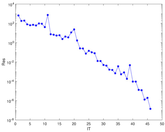
Applying for Algorithm 1, the IT is 46, the CPU time is 3.9496 s and the Res is $1.2885\times {10}^{-6}$. Figure 1 illustrates that Algorithm 1 is feasible.

Example 2 

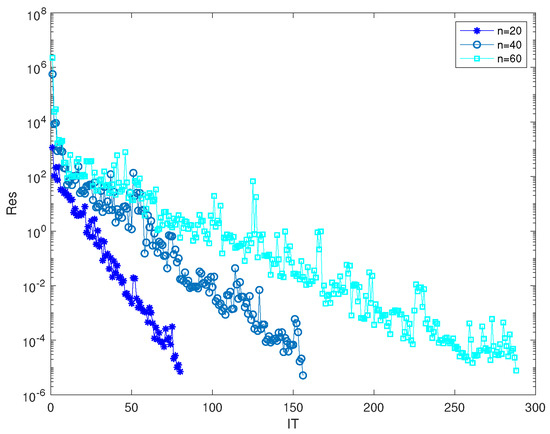
(Test matrices from [28]). We examine the quaternion tensor Equation (2) under the condition that

$$A^{\left(m\right)}=A_{m1}+A_{m2}\mathbf{i}+A_{m3}\mathbf{j}+A_{m4}\mathbf{k},B^{\left(m\right)}=B_{m1}+B_{m2}\mathbf{i}+B_{m3}\mathbf{j}+B_{m4}\mathbf{k},m=1,2,3,$$

where

$$\begin{array}{cc}& A_{11}=triu\left(hilb\left(n\right)\right),A_{12}=triu\left(ones(n,n)\right),A_{13}=eye\left(n\right),A_{14}=ones\left(n\right),\hfill \\ & A_{21}=zeros\left(n\right),A_{22}=zeros\left(n\right),A_{23}=tridiag(-1,2,-1,n),A_{24}=zeros\left(n\right),\hfill \\ & A_{31}=zeros\left(n\right),A_{32}=tridiag(0.5,6,-0.5,n),A_{33}=eye\left(n\right),A_{34}=zeros\left(n\right),\hfill \end{array}$$

$$\begin{array}{cc}& B_{11}=eye\left(n\right),B_{12}=ones\left(n\right),B_{13}=zeros\left(n\right),B_{14}=zeros\left(n\right),\hfill \\ & B_{21}=zeros\left(n\right),B_{22}=tridiag(0.5,6,-0.5,n),B_{23}=eye\left(n\right),B_{24}=zeros\left(n\right),\hfill \\ & B_{31}=tridiag(0.5,6,-0.5,n),B_{32}=eye\left(n\right),B_{33}=zeros\left(n\right),B_{34}=ones\left(n\right).\hfill \end{array}$$

$$\mathcal{C}=tenrand(n,n,n)+tenrand(n,n,n)\mathbf{i}+tenrand(n,n,n)\mathbf{j}+tenrand(n,n,n)\mathbf{k}.$$

Choosingthe initial tensor $\mathcal{X}=\mathcal{Y}=0$, we illustrate the convergence curves of Algorithm 1 for various values of n in Figure 2. In

Table 2. Numerical results for Example 2.

n	IT	CPU Time	Res
20	82	8.3272	$7.7182\times {10}^{-6}$
40	156	24.8187	$5.1233\times {10}^{-6}$
60	288	91.4387	$7.6898\times {10}^{-6}$

, for $n=20,$ $n=40$ and $n=60$, we provide the CPU time incurred, residual norms after a finite number of steps, and the relative errors of the approximate solutions obtained using Algorithm 1.

Example 3. 

We consider the solution of the following convection–diffusion equation over the quaternion algebra [56]

$$\begin{array}{cc}\hfill -v\Delta u+c^T\nabla u& =f\mathit{in}\Gamma =[0,1]\times [0,1]\times [0,1]\hfill \\ \hfill u& =0\mathit{on}\partial \Gamma .\hfill \end{array}$$

Based on a standard finite difference discretization on a uniform grid for the diffusion term and a second-order convergent scheme (Fromm’s scheme) for the convection term with the mesh-size $h={\displaystyle \frac{1}{l+1}}$, we solve the quaternion tensor Equation (3) with

$$A^{\left(n\right)}=A_1^{\left(n\right)}+A_2^{\left(n\right)}\mathbf{i}+A_3^{\left(n\right)}\mathbf{j}+A_4^{\left(n\right)}\mathbf{k},n=1,2,3,$$

where

$$\begin{array}{c}\hfill A_i^{\left(n\right)}={\displaystyle \frac{v_i^{\left(n\right)}}{h^2}}{\left[\begin{array}{ccccc}2& -1& & & \\ -1& 2& -1& & \\ & \ddots & \ddots & \ddots & \\ & & -1& 2& -1\\ & & & -1& 2\end{array}\right]}_{l\times l}+{\displaystyle \frac{c_i^{\left(n\right)}}{4h}}{\left[\begin{array}{ccccc}3& -5& 1& & \\ 1& 3& -5& & \\ & \ddots & \ddots & \ddots & 1\\ & & 1& 3& -5\\ & & & 1& 3\end{array}\right]}_{l\times l},\end{array}$$

and $i=1,2,3,4.$ The right-hand side tensor $\mathcal{C}$ is constructed so that the exact solution to Equation (3) is ${\mathcal{X}}^{*}={\mathcal{X}}_1^{*}+{\mathcal{X}}_2^{*}\mathbf{i}+{\mathcal{X}}_3^{*}\mathbf{j}+{\mathcal{X}}_4^{*}\mathbf{k}=tenones(l,l,l)+tenones(l,l,l)\mathbf{i}+tenones(l,l,l)\mathbf{j}+tenones(l,l,l)\mathbf{k}$.

We consider two cases in order to compare Algorithm 1 with the CGLS algorithm in [43]. In case I, we choose different $v_i^{\left(n\right)}$ and $c_i^{\left(n\right)}$ to obtain the results. In

Table 3. CPU time (IT) for Example 3 with parameter setup in (20).

	l = 10	l = 25	l = 30
Algorithm 1	25.6884(320)	140.8233(1270)	202.7709(1580)
CGLS [43]	15.5685(219)	144.3166(1266)	230.7340(1832)

, we set

$$\begin{array}{c}\hfill v_i^{\left(1\right)}=1,c_i^{\left(1\right)}=1;v_i^{\left(2\right)}=1,c_i^{\left(2\right)}=2;v_i^{\left(3\right)}=1,c_i^{\left(2\right)}=3,i=1,2,3,4\end{array}$$

(20)

to obtain ${\mathcal{A}}^{\left(n\right)}(n=1,2,3)$ with the same real part and imaginary part. In

Table 4. CPU time (IT) for Example 3 with parameter setup in (21).

	l = 10	l = 15	l = 20
Algorithm 1	45.4157(576)	104.4370(1095)	163.6110(1700)
CGLS [43]	44.0701(579)	118.2419(1296)	230.7978(2298)

, we set

$$\begin{array}{cc}\hfill & v_i^{\left(1\right)}=1,c_1^{\left(1\right)}=1,c_2^{\left(1\right)}=-1,c_3^{\left(1\right)}=0,c_4^{\left(1\right)}=1;\hfill \\ \hfill & v_i^{\left(2\right)}=0.1,c_1^{\left(2\right)}=-1,c_2^{\left(2\right)}=-1,c_3^{\left(2\right)}=1,c_4^{\left(2\right)}=0;\hfill \\ \hfill & v_i^{\left(3\right)}=0.01,c_1^{\left(3\right)}=1,c_2^{\left(3\right)}=1,c_3^{\left(3\right)}=0,c_4^{\left(3\right)}=0,i=1,2,3,4\hfill \end{array}$$

(21)

to obtain ${\mathcal{A}}^{\left(n\right)}(n=1,2,3)$ with different real parts and imaginary parts.

In case II, we set $c_i^{\left(1\right)}=1;c_i^{\left(2\right)}=2;c_i^{\left(2\right)}=3,i=1,2,3,4$, we apply Algorithm 1 and the CGLS algorithm in [43] with $v_i^{\left(j\right)}={10}^{-3},1,100,i=1,2,3,4,j=1,2,3$ for grid $10\times 10\times 10$. The relative errors of approximate solution ${\sum }_{i=1}^{i=4}\parallel {\mathcal{X}}_i\left(k\right)-{\mathcal{X}}_i^{*}\parallel /\parallel {\mathcal{X}}_i^{*}\parallel$ computed by these methods are shown in

Table 5. The relative errors of the solution (IT) for Example 3.

	${\mathit{v}}_{\mathit{i}}^{\left(1\right)}={10}^{-3}$	${\mathit{v}}_{\mathit{i}}^{\left(2\right)}=1$	${\mathit{v}}_{\mathit{i}}^{\left(3\right)}=100$
Algorithm 1	$5.6210\times {10}^{-9}$(248)	$6.0527\times {10}^{-9}$(188)	$4.1925\times {10}^{-9}$(248)
CGLS [43]	$9.9300\times {10}^{-9}$(106)	$9.7035\times {10}^{-9}$(178)	$8.9552\times {10}^{-9}$(167)

.

The previous results show that Algorithm 1 has faster convergent rates than the CGLS algorithm in [43] as p increases.

Example 4. 

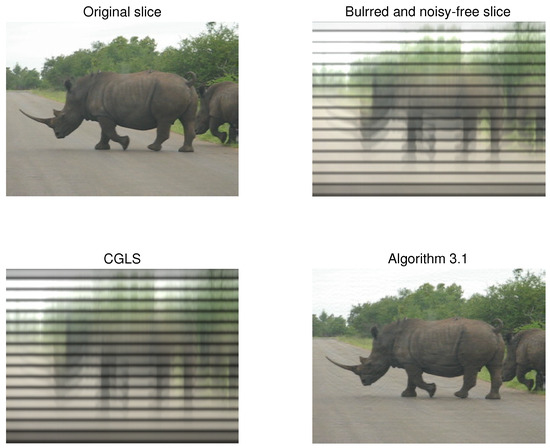
We employ Algorithm 1 to compare its performance with the CGLS algorithm in restoring a color video comprising a sequence of RGB images (slices). The video, titled ‘Rhinos,’ originates from Matlab and is saved in AVI format. Each frontal slice of this color video is represented by a pure quaternion matrix with dimensions of $240\times 320$ pixels. For $\mathcal{C}=\widehat{\mathcal{C}}+\mathcal{N}=\mathcal{X}{\times }_{1}A$, we consider $\mathcal{X}$ to represent the orginal colour video, A as the blurred matrix, and $\mathcal{N}$ as a noise tensor. When $\mathcal{N}=0$, $\mathcal{C}$ is referred to as the blurred and noise-free color video. In this scenario, we select a blurred matrix $A=A_1\otimes A_2\in {\mathbb{R}}^{240\times 320}$, where $A_1={\left(a_{ij}^{\left(1\right)}\right)}_{1\le i,j\le 16}$ and $A_2={\left(a_{ij}^{\left(2\right)}\right)}_{1\le i\le 15,1\le j\le 20}$ are Toeplitz matrices with entries defined as follows:

$$a_{ij}^{\left(1\right)}=\left\{\begin{array}{cc}{\displaystyle \frac{1}{\sigma \sqrt{2\pi }}}exp\left({\displaystyle \frac{{(i-j)}^2}{2{\sigma }^2}}\right),\hfill & |i-j|\le r,\hfill \\ 1,\hfill & \mathit{otherwise}.\hfill \end{array};a_{ij}^{\left(2\right)}=\left\{\begin{array}{cc}{\displaystyle \frac{1}{2s-1}},\hfill & |i-j|\le s,\hfill \\ 0,\hfill & \mathit{otherwise}.\hfill \end{array}\right.\right.$$

We denote ${\mathcal{X}}_{\mathit{restored}}$ as the resulting restored color video. The performance of the algorithm is evaluated using the peak signal-to-noise ratio (PSNR), which is measured in decibels (dB):

$$PSNR\left(\mathcal{X}\right)=10{log}_{10}\left({\displaystyle \frac{I_1{I}_2{d}^2}{{∥\mathcal{X}-{\mathcal{X}}_{\mathit{restored}}∥}^2}}\right),$$

where d denotes the maximum possible pixel value of the image. $RE\left(\mathcal{X}\right)$ represents the relative error, which is defined as

$$RE\left(\mathcal{X}\right)={\displaystyle \frac{∥\mathcal{X}-{\mathcal{X}}_{\mathit{restored}}∥}{\parallel \mathcal{X}\parallel }}.$$

In this case, we use $d=255$ and set the variance $\sigma =1$.

Table 6. The numerical results for Example 4.

Algorithm([r,s])	Algorithm 1(PSNR/RE)	CGLS(PSNR/RE)
[3,3]	38.6181(0.0235)	13.8404(0.3769)
[6,6]	37.3721(0.0300)	14.0529(0.3694)
[8,8]	33.8073(0.0338)	14.7958(0.3551)

shows the peak signal-to-noise ratio (PSNR) and the relative error (RE) for Algorithm 1 and the CGLS algorithm with various parameters. As indicated, the PSNR and the relative error of our algorithms are significantly superior to those of CGLS. For the case where $r=6$ and $s=6$ with slice No. 7 of the color video, we illustrate the original image, blurred image, and the restored image by CGLS and Algorithm 1 in Figure 3. This figure demonstrates that our algorithm can effectively restore blurred and noise-free color video with high quality.

5. Conclusions

The main goal of this paper is to solve the generalized quaternion tensor Equation (2). We hereby develop a BiCG iterative algorithm in tensor format to efficiently solve Equation (2), and we also prove the convergence of our proposed method. Moreover, we demonstrate that the solution with a minimal Frobenius norm can be achieved by initializing specific types of tensors. We provide several examples to effectively illustrate the effectiveness of our algorithm. Furthermore, our algorithm is successfully applied to the restoration of color videos. This contribution significantly advances the current understanding of quaternion tensor equations by introducing a practical iterative approach.

References

- Kolda, T.G.; Bader, B.W. Tensor decompositions and applications. SIAM Rev. 2009, 51, 455–500. [Google Scholar] [CrossRef]
- Qi, L.; Luo, Z. Tensor Analysis: Spectral Theory and Special Tensors; SIAM: Philadelphia, PA, USA, 2017. [Google Scholar]
- Beik, F.P.; Jbilou, K.; Najafi-Kalyani, M.; Reichel, L. Golub–Kahan bidiagonalization for ill-conditioned tensor equations with applications. Numer. Algorithms 2020, 84, 1535–1563. [Google Scholar] [CrossRef]
- Duan, X.F.; Zhang, Y.S.; Wang, Q.W. An efficient iterative method for solving a class of constrained tensor least squares problem. Appl. Numer. Math. 2024, 196, 104–117. [Google Scholar] [CrossRef]
- Guan, Y.; Chu, D. Numerical computation for orthogonal low-rank approximation of tensors. SIAM J. Matrix Anal. Appl. 2019, 40, 1047–1065. [Google Scholar] [CrossRef]
- Guan, Y.; Chu, M.T.; Chu, D. Convergence analysis of an SVD-based algorithm for the best rank-1 tensor approximation. Linear Algebra Appl. 2018, 555, 53–69. [Google Scholar] [CrossRef]
- Guan, Y.; Chu, M.T.; Chu, D. SVD-based algorithms for the best rank-1 approximation of a symmetric tensor. SIAM J. Matrix Anal. 2018, 39, 1095–1115. [Google Scholar] [CrossRef]
- Hu, J.; Ke, Y.; Ma, C. Efficient iterative method for generalized Sylvester quaternion tensor equation. Comput. Appl. Math. 2023, 42, 237. [Google Scholar] [CrossRef]
- Ke, Y. Finite iterative algorithm for the complex generalized Sylvester tensor equations. J. Appl. Anal. Comput. 2020, 10, 972–985. [Google Scholar] [CrossRef]
- Kolda, T.G. Multilinear Operators for Higher-Order Decompositions; Sandia National Laboratory (SNL): Albuquerque, NM, USA; Livermore, CA, USA, 2006. [Google Scholar]
- Li, B.W.; Tian, S.; Sun, Y.S.; Hu, Z.M. Schur-decomposition for 3D matrix equations and its application in solving radiative discrete ordinates equations discretized by Chebyshev collocation spectral method. J. Comput. Phys. 2010, 229, 1198–1212. [Google Scholar] [CrossRef]
- Li, T.; Wang, Q.-W.; Duan, X.-F. Numerical algorithms for solving discrete Lyapunov tensor equation. J. Comput. Appl. Math. 2020, 370, 112676. [Google Scholar] [CrossRef]
- Li, T.; Wang, Q.-W.; Zhang, X.-F. Gradient based iterative methods for solving symmetric tensor equations. Numer. Linear Algebra Appl. 2022, 29, e2414. [Google Scholar] [CrossRef]
- Li, T.; Wang, Q.-W.; Zhang, X.-F. A Modified conjugate residual method and nearest kronecker product preconditioner for the generalized coupled Sylvester tensor equations. Mathematics 2022, 10, 1730. [Google Scholar] [CrossRef]
- Li, X.; Ng, M.K. Solving sparse non-negative tensor equations: Algorithms and applications. Front. Math. China 2015, 10, 649–680. [Google Scholar] [CrossRef]
- Liang, Y.; Silva, S.D.; Zhang, Y. The tensor rank problem over the quaternions. Linear Algebra Appl. 2021, 620, 37–60. [Google Scholar] [CrossRef]
- Lv, C.; Ma, C. A modified CG algorithm for solving generalized coupled Sylvester tensor equations. Appl. Math. Comput. 2020, 365, 124699. [Google Scholar] [CrossRef]
- Malek, A.; Momeni-Masuleh, S.H. A mixed collocation–finite difference method for 3D microscopic heat transport problems. J. Comput. Appl. Math. 2008, 217, 137–147. [Google Scholar] [CrossRef][Green Version]
- Qi, L. Eigenvalues of a real supersymmetric tensor. J. Symb. Comput. 2005, 40, 1302–1324. [Google Scholar] [CrossRef]
- Qi, L. Symmetric nonnegative tensors and copositive tensors. Linear Algebra Appl. 2013, 439, 228–238. [Google Scholar] [CrossRef]
- Qi, L.; Chen, H.; Chen, Y. Tensor Eigenvalues and Their Applications; Springer: Berlin/Heidelberg, Germany, 2018. [Google Scholar]
- Zhang, X.-F.; Li, T.; Ou, Y.-G. Iterative solutions of generalized Sylvester quaternion tensor equations. Linear Multilinear Algebra 2024, 72, 1259–1278. [Google Scholar] [CrossRef]
- Zhang, X.-F.; Wang, Q.-W. On RGI Algorithms for Solving Sylvester Tensor Equations. Taiwan. J. Math. 2022, 26, 501–519. [Google Scholar] [CrossRef]
- Kyrchei, I. Cramer’s rules for Sylvester quaternion matrix equation and its special cases. Adv. Appl. Clifford Algebras 2018, 28, 1–26. [Google Scholar] [CrossRef]
- Heyouni, M.; Saberi-Movahed, F.; Tajaddini, A. On global Hessenberg based methods for solving Sylvester matrix equations. Comput. Math. Appl. 2019, 77, 77–92. [Google Scholar] [CrossRef]
- Zhang, X. A system of generalized Sylvester quaternion matrix equations and its applications. Appl. Math. Comput. 2016, 273, 74–81. [Google Scholar] [CrossRef]
- Beik, F.; Ahmadi-Asl, S. An iterative algorithmfor η-(anti)-Hermitian least-squares solutions of quaternion matrix equations. Electron. J. Linear Algebra 2015, 30, 372–401. [Google Scholar] [CrossRef]
- Ahmadi-Asl, S.; Beik, F.P.A. An efficient iterative algorithm for quaternionic least-squares problems over the generalized η-(anti-)bi-Hermitian matrices. Linear Multilinear Algebra 2017, 65, 1743–1769. [Google Scholar] [CrossRef]
- Ahmadi-Asl, S.; Beik, F.P.A. Iterative algorithms for least-squares solutions of a quaternion matrix equation. J. Appl. Math. Comput. 2017, 53, 95–127. [Google Scholar] [CrossRef]
- Song, G.; Wang, Q.-W.; Yu, S. Cramer’s rule for a system of quaternion matrix equations with applications. Appl. Math. Comput. 2018, 336, 490–499. [Google Scholar] [CrossRef]
- Wang, Q.-W.; He, Z.-H.; Zhang, Y. Constrained two-sided coupled Sylvester-type quaternion matrix equations. Automatica 2019, 101, 207–213. [Google Scholar] [CrossRef]
- Zhang, F.; Mu, W.; Li, Y.; Zhao, J. Special least squares solutions of the quaternion matrix equation AXB + CXD = E. Comput. Math. Appl. 2016, 72, 1426–1435. [Google Scholar] [CrossRef]
- Huang, N.; Ma, C.-F. Modified conjugate gradient method for obtaining the minimum-norm solution of the generalized coupled Sylvester-conjugate matrix equations. Appl. Math. Model. 2016, 40, 1260–1275. [Google Scholar] [CrossRef]
- Gao, Z.-H.; Wang, Q.-W.; Xie, L. The (anti-)η-Hermitian solution to a novel system of matrix equations over the split quaternion algebra. Math. Meth. Appl. Sci. 2024, 1–18. [Google Scholar] [CrossRef]
- He, Z.-H.; Wang, X.-X.; Zhao, Y.-F. Eigenvalues of quaternion tensors with applications to color video processing. J. Sci. Comput. 2023, 94, 1. [Google Scholar] [CrossRef]
- Jia, Z.; Wei, M.; Zhao, M.X.; Chen, Y. A new real structure-preserving quaternion QR algorithm. J. Comput. Appl. Math. 2018, 343, 26–48. [Google Scholar] [CrossRef]
- Li, Y.; Wei, M.; Zhang, F.; Zhao, J. Real structure-preserving algorithms of Householder based transformations for quaternion matrices. J. Comput. Appl. Math. 2016, 305, 82–91. [Google Scholar] [CrossRef]
- Mehany, M.S.; Wang, Q.-W.; Liu, L. A System of Sylvester-like quaternion tensor equations with an application. Front. Math. 2024, 19, 749–768. [Google Scholar] [CrossRef]
- Xie, M.; Wang, Q.-W. Reducible solution to a quaternion tensor equation. Front. Math. China 2020, 15, 1047–1070. [Google Scholar] [CrossRef]
- Xie, M.Y.; Wang, Q.W.; He, Z.H.; Saad, M.M. A system of Sylvester-type quaternion matrix equations with ten variables. Acta Math. Sin. (Engl. Ser.) 2022, 38, 1399–1420. [Google Scholar] [CrossRef]
- Saberi-Movahed, F.; Tajaddini, A.; Heyouni, M.; Elbouyahyaoui, L. Some iterative approaches for Sylvester tensor equations, Part I: A tensor format of truncated Loose Simpler GMRES. Appl. Numer. Math. 2022, 172, 428–445. [Google Scholar] [CrossRef]
- Saberi-Movahed, F.; Tajaddini, A.; Heyouni, M.; Elbouyahyaoui, L. Some iterative approaches for Sylvester tensor equations, Part II: A tensor format of Simpler variant of GCRO-based methods. Appl. Numer. Math. 2022, 172, 413–427. [Google Scholar] [CrossRef]
- Wang, Q.-W.; Xu, X.; Duan, X. Least squares solution of the quaternion Sylvester tensor equation. Linear Multilinear Algebra 2021, 69, 104–130. [Google Scholar] [CrossRef]
- Zhang, X.-F.; Wang, Q.-W. Developing iterative algorithms to solve Sylvester tensor equations. Appl. Math. Comput. 2021, 409, 126403. [Google Scholar] [CrossRef]
- Chen, Z.; Lu, L. A projection method and Kronecker product preconditioner for solving Sylvester tensor equations. Sci. China Math. 2012, 55, 1281–1292. [Google Scholar] [CrossRef]
- Karimi, S.; Dehghan, M. Global least squares method based on tensor form to solve linear systems in Kronecker format. Trans. Inst. Measure. Control 2018, 40, 2378–2386. [Google Scholar] [CrossRef]
- Najafi-Kalyani, M.; Beik, F.P.A.; Jbilou, K. On global iterative schemes based on Hessenberg process for (ill-posed) Sylvester tensor equations. J. Comput. Appl. Math. 2020, 373, 112216. [Google Scholar] [CrossRef]
- Bai, Z.-Z.; Golub, G.H.; Ng, M.K. Hermitian and skew-Hermitian splitting methods for non-Hermitian positive definite linear systems. SIAM J. Matrix Anal. Appl. 2003, 24, 603–626. [Google Scholar] [CrossRef]
- Grasedyck, L. Existence and computation of low Kronecker-rank approximations for large linear systems of tensor product structure. Computing 2004, 72, 247–265. [Google Scholar] [CrossRef]
- Peng, Y.; Hu, X.; Zhang, L. An iteration method for the symmetric solutions and the optimal approximation solution of the matrix equation AXB = C. Appl. Math. Comput. 2005, 160, 763–777. [Google Scholar] [CrossRef]
- Bank, R.E.; Chan, T.-F. An analysis of the composite step biconjugate gradient method. Numer. Math. 1993, 66, 295–319. [Google Scholar] [CrossRef]
- Bank, R.E.; Chan, T.-F. A composite step bi-conjugate gradient algorithm for nonsymmetric linear systems. Numer. Algorithms 1994, 7, 1–16. [Google Scholar] [CrossRef]
- Freund, R.W.; Golub, G.H.; Nachtigal, N.M. Iterative solution of linear systems. Acta Numer. 1992, 1, 44. [Google Scholar] [CrossRef]
- Hajarian, M. Developing Bi-CG and Bi-CR methods to solve generalized Sylvester-transpose matrix equations. Int. J. Auto. Comput. 2014, 11, 25–29. [Google Scholar] [CrossRef]
- Beik, F.; Panjeh, F.; Movahed, F.; Ahmadi-Asl, S. On the Krylov subspace methods based on tensor format for positive definite Sylvester tensor equations. Numer. Linear Algebra Appl. 2016, 23, 444–466. [Google Scholar] [CrossRef]
- Ballani, J.; Grasedyck, L. A projection method to solve linear systems in tensor format. Numer. Linear Algebra Appl. 2013, 20, 27–43. [Google Scholar] [CrossRef]
Disclaimer/Publisher’s Note: The statements, opinions and data contained in all publications are solely those of the individual author(s) and contributor(s) and not of MDPI and/or the editor(s). MDPI and/or the editor(s) disclaim responsibility for any injury to people or property resulting from any ideas, methods, instructions or products referred to in the content. |
© 2024 by the authors. Licensee MDPI, Basel, Switzerland. This article is an open access article distributed under the terms and conditions of the Creative Commons Attribution (CC BY) license (https://creativecommons.org/licenses/by/4.0/).