Research on Small Sample Rolling Bearing Fault Diagnosis Method Based on Mixed Signal Processing Technology

Abstract

The diagnosis of bearing faults is a crucial aspect of ensuring the optimal functioning of mechanical equipment. However, in practice, the use of small samples and variable operating conditions may result in suboptimal generalization performance, reduced accuracy, and overfitting for these methods. To address this challenge, this study proposes a bearing fault diagnosis method based on a symmetric two-stream convolutional neural network (CNN). The method employs hybrid signal processing techniques to address the issue of limited data. The method employs a symmetric parallel convolutional neural network (CNN) for the analysis of bearing data. Initially, the data are transformed into time–frequency maps through the utilization of the short-time Fourier transform (STFT) and the simultaneous compressed wavelet transform (SCWT). Subsequently, two sets of one-dimensional vectors are generated by reconstructing the high-resolution features of the faulty samples using a symmetric parallel convolutional neural network (CNN). Feature splicing and fusion are then performed to generate bearing fault diagnosis information and assist fault classification. The experimental results demonstrate that the proposed mixed-signal processing method is effective on small-sample datasets, and verify the feasibility and generality of the symmetric parallel CNN-support vector machine (SVM) model for bearing fault diagnosis under small-sample conditions.

1. Introduction

Considering the ever-evolving and intricate environments where large machinery and equipment function, maintaining their daily functionality is crucial for the equipment’s stability [1]. Bearing failure, as an essential element of the mechanical transmission system, frequently contributes significantly to the overall breakdown of mechanical equipment [2]. The vibration and vibration suppression of bearings has been an important research area in recent decades [3]. Due to its critical role, bearing failure often becomes a primary factor in the complete failure of such systems [4]. Therefore, identifying bearing malfunctions is crucial for sustaining the peak performance of mechanical equipment [5]. Traditional approaches for identifying faults, including support vector machines (SVMs), extreme learning machines (ELMs), and other diagnostic techniques, are employed to detect bearing issues [6]. Extreme learning machine (ELM), empirical modal decomposition (EMD) [7], empirical mode decomposition (EMD) [8], etc., have achieved good results in bearing fault diagnosis. Compared to traditional methods, deep learning offers advanced abilities in extracting features from complex sensor data and handling large, high-dimensional datasets. As a result, it shows significant potential in bearing fault diagnosis. In this field [9], the techniques based on deep learning have proven to be highly effective for diagnostic purposes. At present, a number of deep learning networks have been employed in the domain of fault diagnosis [10]. Ni et al. [11] proposed a novel approach for rolling bearing fault diagnosis, which involves an adaptive deep confidence network. This network integrates principal component analysis and utilizes a linear unit activation layer with parameter adjustment. This approach effectively extracts fault information and enables accurate diagnosis. In a previous study, Li et al. [12] proposed a model that combined a recurrent neural network with double-order attention and a convolutional attention module. This model demonstrated promising results when tested on the rolling bearing dataset. Wanyu Liu and colleagues [13] proposed a model that combines a deep convolutional neural network with a broad convolutional kernel and a deep long- and short-term memory network. This approach is designed to address the challenge of temporal data in fault diagnosis. In the study [14], a one-dimensional convolutional neural network (CNN) was employed to process one-dimensional signals. This approach enabled the real-time detection of motor faults by utilizing both feature extraction and classification techniques.

In recent years, the field of small sample learning has garnered significant interest from a diverse array of researchers, with a multitude of novel approaches emerging, including data augmentation, self-supervised learning, transfer learning, and meta-learning [15]. In the context of limited data, the aforementioned methods offer novel solutions to the challenge of small sample sizes. Huang et al. [16] employed a multi-source domain adaptive approach with dense convolutions and fused convolutional blocks for deep feature extraction and fusion. This approach demonstrated robust diagnostic capabilities and yielded promising results. Hu et al. [17] put forth a task-ordering meta-learning approach which clusters tasks in order from simple to complex and classifies new categories in data-scarce scenarios. Wang et al. [18] integrated a wavelet network with a prototype network to facilitate the diagnosis of bearing faults. This approach enabled the accurate identification of previously unused categories during the training phase.

Typically, before determining the exact type of fault, the aforementioned methods use signal processing techniques to derive relevant features from the raw vibration data [19]. However, in actual working conditions, the probability of bearing faults occurring is extremely low, so collecting sufficient fault samples becomes difficult. In the event that a deep learning model is not sufficiently trained with a sufficient number of samples, the phenomenon of overfitting can occur with ease, which subsequently results in a notable reduction in the model’s performance [20]. In the event that the data samples are insufficient or unbalanced, it becomes challenging to accurately discern the various faults. This is due to the fact that the categories with a paucity of data samples are prone to being overlooked and overshadowed by those with a plethora of data samples [21]. In their study, the authors of [22] put forth a novel data augmentation approach based on raw data. This technique involves splitting a sample into multiple monomers, which are then reorganized to increase the number of data samples. By using this method, the sample size can be greatly increased, leading to significant improvements in feature learning and classification results. In this study [23], we introduce a fault diagnosis method designed for unbalanced data using a Conditional Deep Convolutional Generative Adversarial Network (C-DCGAN) model. This model exploits the feature extraction strengths of convolutional networks while incorporating conditional support [24]. By using generative samples as augmented data, our approach optimizes structural elements for improved machine fault diagnosis [25]. This method aims to increase fault diagnosis accuracy, especially when sample sizes are limited, and to improve the generalizability of the classifier [26].

In [27], a WGAN-based approach is proposed as a means of artificially synthesizing new samples of labeled fault types. Specifically, the method uses WGAN to identify defect sample distributions and generate new samples for deep network training. This technique facilitates both the growth and improvement of the training dataset. To efficiently extract classification features and train the model, a one-dimensional convolutional neural network (1D-CNN) is applied to both the original and generated samples [28]. The results obtained in fault diagnosis are both remarkable and satisfactory. To address the problem of insufficient data in bearing fault diagnosis, the described methods have shown promising results [29]. However, they also exhibit certain limitations: ① The aforementioned methodologies are founded upon one-dimensional signals for the purpose of diagnosing faults [30]. However, this approach is unable to fully leverage the capabilities of two-dimensional convolutional neural networks (2D-CNNs) for image generation. Additionally, the generated samples exhibit a lack of quality and diversity. ② The analysis does not fully leverage the information embedded in the vibration signals across both the time and frequency domains [31].

Coping strategies for current small sample problems:

• Migration learning: The method employs models that have been pre-trained on large-scale datasets and subsequently fine-tuned to accommodate small sample datasets. This approach fully exploits the existing knowledge and mitigates the reliance on limited sample datasets [32].
• Generative Adversarial Networks (GANs): It is possible to enhance the diversity of the sample set by developing models that can generalize more effectively when dealing with smaller sample sizes. Generative Adversarial Networks (GANs) can create virtual samples that resemble real ones, allowing the training dataset to be expanded [33].
• Feature selection and dimensionality reduction: In a limited number of samples, feature selection and transformed dimensionality techniques remove redundant information and retain the most useful features for fault diagnosis, improving model performance [34].

The objective of this study is to integrate two key techniques, namely the short-time Fourier transform and the synchronized compressed wavelet transform. The primary objective of the integration is to eliminate redundant information through the application of feature selection and dimensionality reduction techniques, thereby enhancing the accuracy of fault diagnosis in the context of limited sample sizes by focusing on the most pertinent features. Subsequently, the processed bearing data are evaluated using a two-stream convolutional neural network (CNN) model with symmetry in both branches, in conjunction with a support vector machine (SVM) model. This paper presents a novel mixed-signal processing method to address the challenges posed by limited fault sample data and uncertain fault classification. The method converts a one-dimensional time series into a two-dimensional image, thereby preserving the essential characteristics of the original signal, thus enhancing the accuracy of the fault diagnosis through the combined CNN-SVM model.

This paper is structured as follows: Section 2 introduces the related theories of the signal processing methods short-time Fourier transform (STFT) and synchronous compressed wavelet transform (SWT), explains the basic principles of parallel convolutional neural networks (CNNs), and describes the structure of the STFT-SWT-PCNN-SVM model in detail. Section 3 provides a detailed account of the algorithmic flow of the STFT-SWT-PCNN-SVM model. Section 4 presents the time–frequency plots processed by the two data processing methods employing the proposed method to identify different sample size cases and to compare the diagnostic results. Additionally, experiments are conducted with different datasets. Section 5 presents the conclusions of this study and offers suggestions for future research.

2. Relevant Methodologies

Complementarity of STFT and SCWT: The selective missing problem in SCWT arises when the choice of wavelet basis functions leads to the omission or distortion of certain frequency components in the signal. This results in the potential loss or alteration of frequency information. In contrast, the short-time Fourier transform (STFT) mitigates this problem to some extent by using a fixed window function whose frequency characteristics match those of the signal. The STFT decomposes the signal into narrow-band components over time and frequency, more effectively preserving the frequency information at each time point. Meanwhile, SCWT excels at multi-scale analysis, providing a more detailed frequency profile by evaluating the signal at different scales compared to STFT. The accuracy and efficiency of signal analysis can be further improved by combining these two methods.

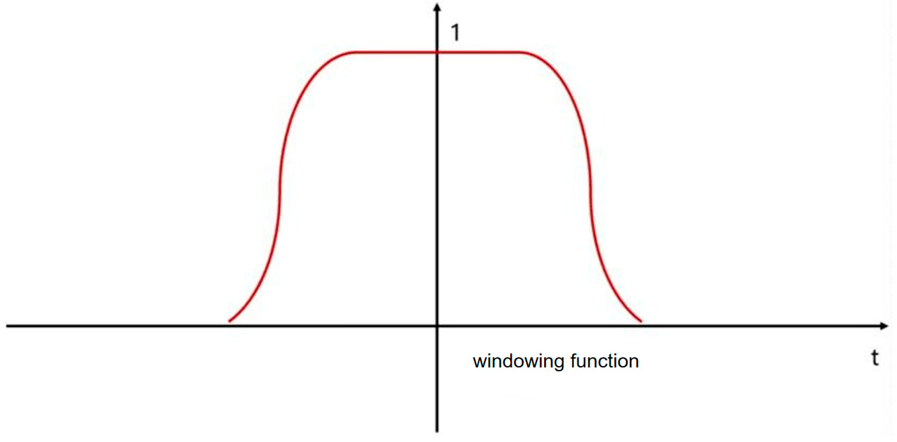
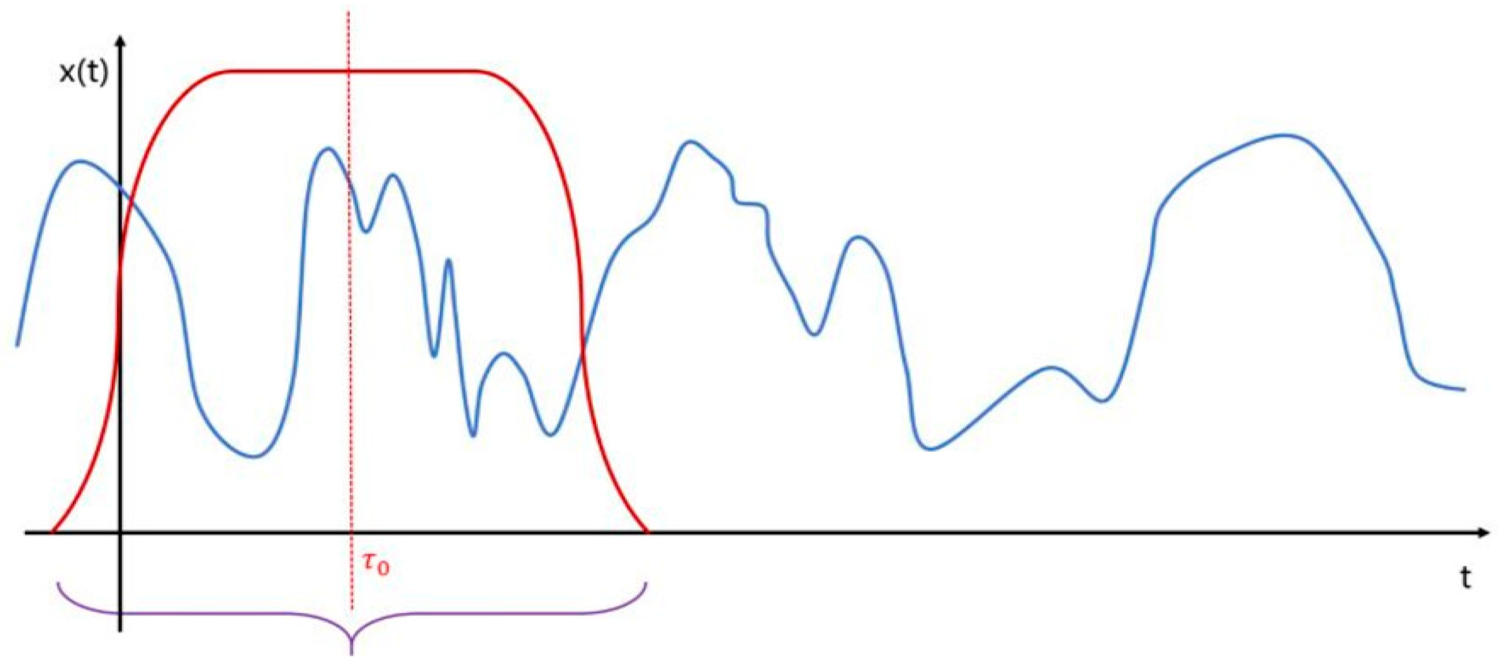
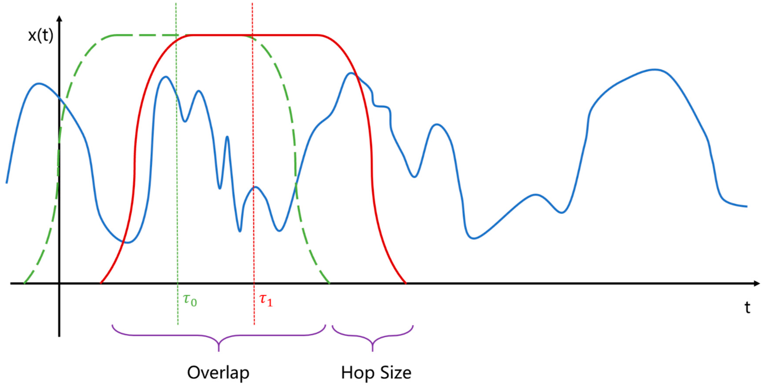
2.1. Short-Time Fourier Transforms

The short-time Fourier transform (STFT) is a time–frequency analysis technique designed to evaluate non-stationary, time-varying signals. It converts a one-dimensional vibration signal into a two-dimensional matrix suitable for processing by convolutional neural networks (CNNs), representing a feature spectrum with time–frequency domain information. This method is an extension of the Fourier transform, which only provides information about signal characteristics in the frequency domain and lacks temporal analysis capabilities [35]. To bridge the gap between the time and frequency domains, Gabor introduced the STFT in 1946, which is essentially a windowed version of the Fourier transform [36]. The STFT process involves applying a finite windowing function, h(t), to the signal before performing the Fourier transform. This approach assumes that the signal is smooth over a short time interval. By analyzing segments of the signal within these smooth intervals using the windowing function, a sequence of local spectra is produced that are then combined to form a two-dimensional time–frequency representation. The short-time Fourier transform of the signal is defined as follows:

First, define a window function $\mathrm{w}\left(\mathrm{t}\right)$.The Define Window function is shown in Figure 1.

The window is then moved to the open position of the signal when the window function is centered at $\left(\mathrm{t}-{\mathsf{\tau }}_0\right)$, and the signal is windowed

$$y\left(t\right)=x\left(t\right)\cdot w\left(t-{\tau }_0\right),$$

(1)

Then, the Fourier transform

$$STFT\left(t,\hspace{0.25em}f\right)={\int }_{-\mathrm{\infty }}^{\mathrm{\infty }}x\left(\tau \right)h\left(\tau -t\right){\mathrm{e}}^{-j2\pi f\tau }\mathrm{d}\tau ,$$

(2)

This gives us the spectral distribution $\mathrm{X}\left(\mathsf{\omega }\right)$ of the first segmented sequence, and in real applications, since the signal is a discrete sequence of points, we obtain the spectral sequence $\mathrm{X}\left(\mathrm{N}\right)$, and for the ease of representation, we define here the function $\mathrm{S}\left(\mathsf{\omega },\mathsf{\tau }\right)$, which denotes, after transforming the original function at the center of the window function, the spectral result $\mathrm{X}\left(\mathsf{\omega }\right)$. The result is as follows:

$$S\left(\omega ,\tau \right)=\mathcal{F}\left(x\left(t\right)\cdot w\left(t-\tau \right)\right)={\int }_{\infty }^{+\infty }x\left(t\right)\cdot w\left(t-\tau \right)e^{-j\omega t}dt,$$

(3)

Corresponding to the discrete scenario, $\mathrm{S}\left(\mathsf{\omega },\mathsf{\tau }\right)$ is a two-dimensional matrix where each column represents the resulting sequence after windowing the signal at different locations and performing a Fourier transform on the resulting segments.

Adding a window for the signal is shown in Figure 2.

After completing the Fourier transform operation on the first segment, move the window function to τ₁. The distance the window is moved is called the Hop size, and the distance is generally less than the width of the window, ensuring that there is some overlap between the front and back of the two windows, which we call the overlap.

The hop size and overlap of the jumps are shown in Figure 3.

We end up with S, which is the result of the STFT transformation.

$$\mathrm{S}\mathrm{T}\mathrm{F}\mathrm{T}\left(\mathsf{\omega },\mathsf{\tau }\right)=\mathcal{F}\left(\mathrm{x}\left(\mathrm{t}\right)\cdot \mathrm{w}\left(\mathrm{t}-\mathsf{\tau }\right)\right)={\int }_{\mathrm{\infty }}^{+\mathrm{\infty }}\mathrm{x}\left(\mathrm{t}\right)\cdot \mathrm{w}\left(\mathrm{t}-\mathsf{\tau }\right){\mathrm{e}}^{{\mathrm{e}}^{-j2\pi f\tau }}\mathrm{d}\mathrm{t},$$

(4)

Eq: $w\left(t-\tau \right)$ is the analysis window function.

Based on the equation provided, the short-time Fourier transform (STFT) of a signal $\mathrm{x}\left(\mathrm{t}\right)$ at a particular time t involves applying a Fourier transform to the signal that has been multiplied by an analysis window $w\left(t-\tau \right)$ centered at t. Essentially, this means that multiplying $\mathrm{x}\left(\mathrm{t}\right)$ by the window function $w\left(t-\tau \right)$ extracts a segment of the signal around the specified time t. At any given time t, the $\mathrm{S}\mathrm{T}\mathrm{F}\mathrm{T}\left(\mathrm{t},\mathrm{f}\right)$ can be interpreted as representing the signal’s spectrum at that precise moment. Specifically, when the window function $\mathrm{w}\left(\mathrm{t}\right)\equiv 1$, the STFT simplifies to a standard Fourier transform. To achieve the best localization in time–frequency analysis, the window function’s width should be adjusted according to the characteristics of the signal—larger windows are suited for sinusoidal signals, while smaller windows are preferable for impulse signals. The STFT has certain advantages and drawbacks: its main benefit lies in the fact that it builds upon the well-understood Fourier transform, making its physical interpretation straightforward; however, its limitation is that the window width remains fixed and cannot be adjusted dynamically.

2.2. Synchronized Compressed Wavelet Transform

The Simultaneous Compressive Wavelet Transform (SCWT) is a method created to enhance the precision of time–frequency representations. It redistributes values across the plane to different time–frequency points, focusing energy within the spectrogram and achieving sparsity. This method corrects the blurring effect typically seen in wavelet transform results, resulting in a more accurate time–frequency distribution and superior video resolution compared to standard wavelet transforms. Essentially, SCWT reorganizes the wavelet coefficients in the time–frequency plane, concentrating the energy near the actual instantaneous frequency. This makes it particularly effective for analyzing signals that change over time and are non-stationary [37]. The wavelet coefficients of the wavelet coefficients are

$$W_f(\alpha ,\beta )={\alpha }^{-1/2}\int {\Psi }^{*}\left({\displaystyle \frac{t-\beta }{\alpha }}\right)f\left(t\right)dt,$$

(5)

In this context, α and β represent the constants that indicate the scale factor and translation factor, respectively. The term refers to the complex conjugate of the wavelet basis. Essentially, it functions as the complex conjugate of the wavelet basis.

For any (α,β), if W(α,β) ≠ 0, then the corresponding instantaneous frequency is as follows:

$${\omega }_f(\begin{array}{c}\alpha ,\beta )\end{array}={\displaystyle \frac{-i\partial W_f(\begin{array}{c}\alpha ,\beta )\end{array}}{\partial \beta W_f(\begin{array}{c}\alpha ,\beta )\end{array}}},$$

(6)

Projecting the wavelet coefficients W(α,β) from the scale plane (α,β) to the time–frequency plane [o(α,β),β], i.e., compressing them to the center frequency w. Around it, one obtains the continuum expression of the SCWT

$$T_j(\begin{array}{c}{\omega }_n,\beta )\end{array}=\hspace{0.25em}{\alpha }^{-3/2}{\int }_{A\left(\beta \right)}{W}_f(\begin{array}{c}\alpha ,\beta )\end{array}\mathrm{d}\alpha ,$$

(7)

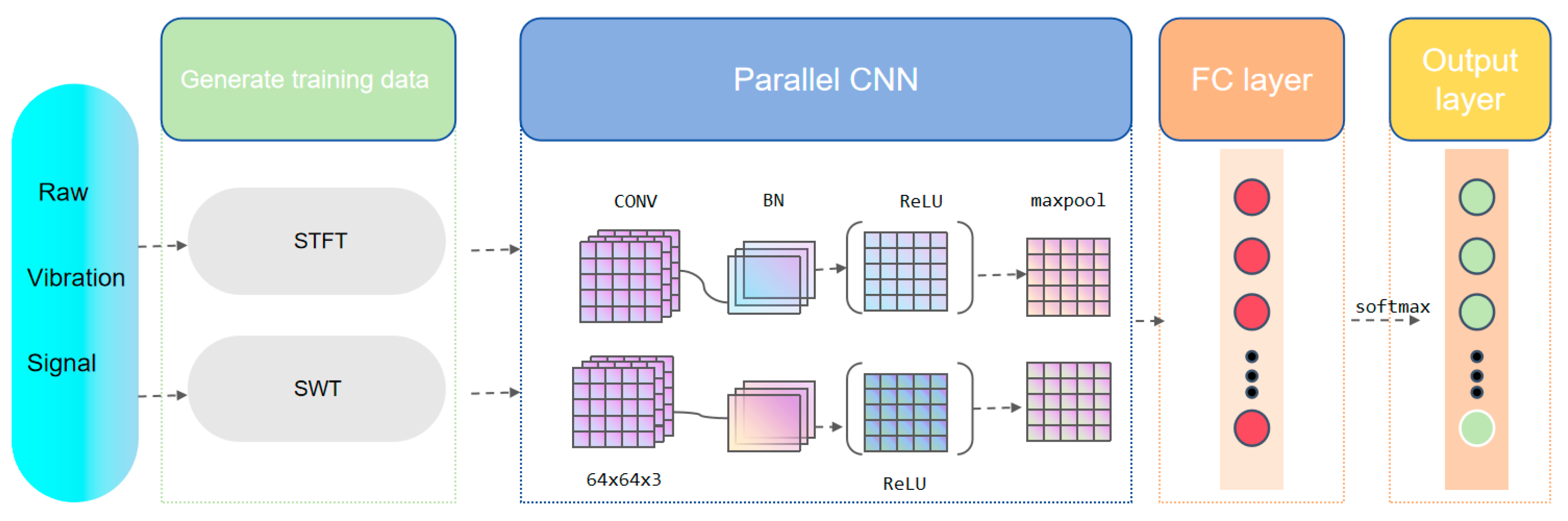
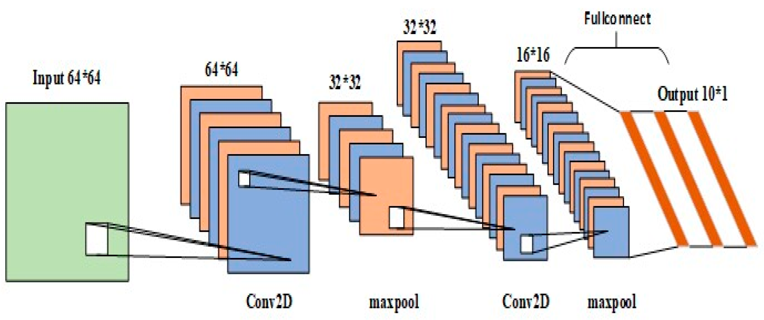
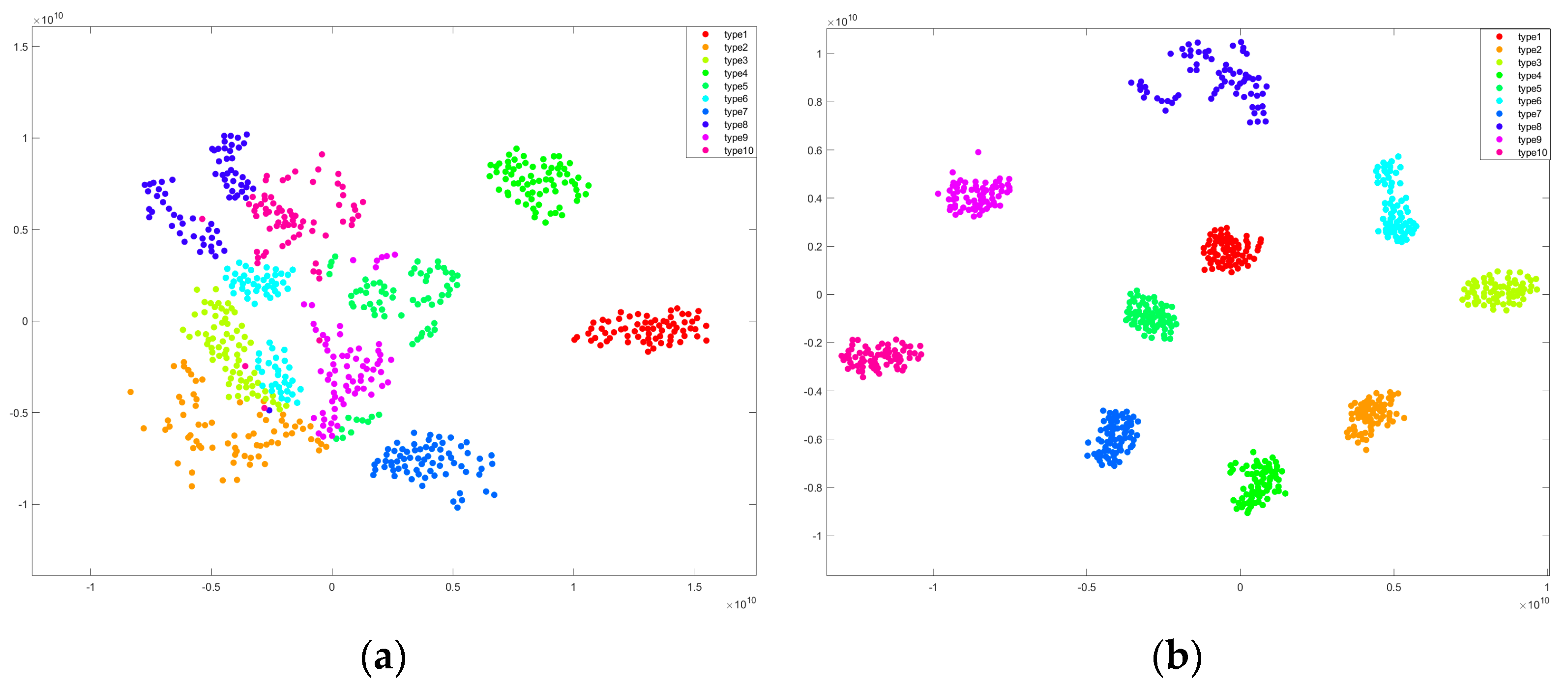
2.3. Dual-Channel Parallel CNN Model with Symmetry

Convolutional neural networks (CNNs) [38] are a type of feed-forward neural network characterized by local connectivity and weight distribution. A CNN is composed of an input layer, convolutional layers, pooling layers, fully connected layers, and an output layer. Traditional fault diagnosis involves feature extraction followed by pattern recognition and classification, often leading to inconsistencies and failing to fully utilize time series fault data [39]. In contrast, CNNs enhance feature differentiation, providing improved accuracy and efficiency, and are increasingly utilized in fault diagnosis. Nevertheless, basic CNN architectures may struggle to capture timing changes in bearing signal faults [40].

The overall structure of the CNN is shown in Figure 4.

In this paper, two symmetric two-channel parallel CNN models are used for training, and the parameters of the two CNNs are all set to be symmetric and consistent.

First, the SFTF image and the SWT image are simultaneously fed into the two parallel CNNs, and after two-layer convolution-pooling and then convolution-pooling (after each convolution operation, batch normalization is performed, and then 2 × 2 max-pooling is performed to remove unnecessary features). Each of the two CNNs outputs a set of one-dimensional vectors; then, the two sets of the output one-dimensional vectors are connected and fused; after passing through the fully connected layer, the fused features are finally fed into the SVM classifier, which outputs the bearing fault diagnosis results.

The structure of the two-channel parallel CNN is shown in Figure 5 below:

3. Diagnostic Methods and Processes

The troubleshooting process in this paper is shown in Figure 6 below.

The intelligent fault diagnosis method model based on SFTF plus SCWT and parallel CNN is trained as follows:

(1)

Data processing: The overlapping intercepts of signals, adding labels, and obtaining sample sets.

(2)

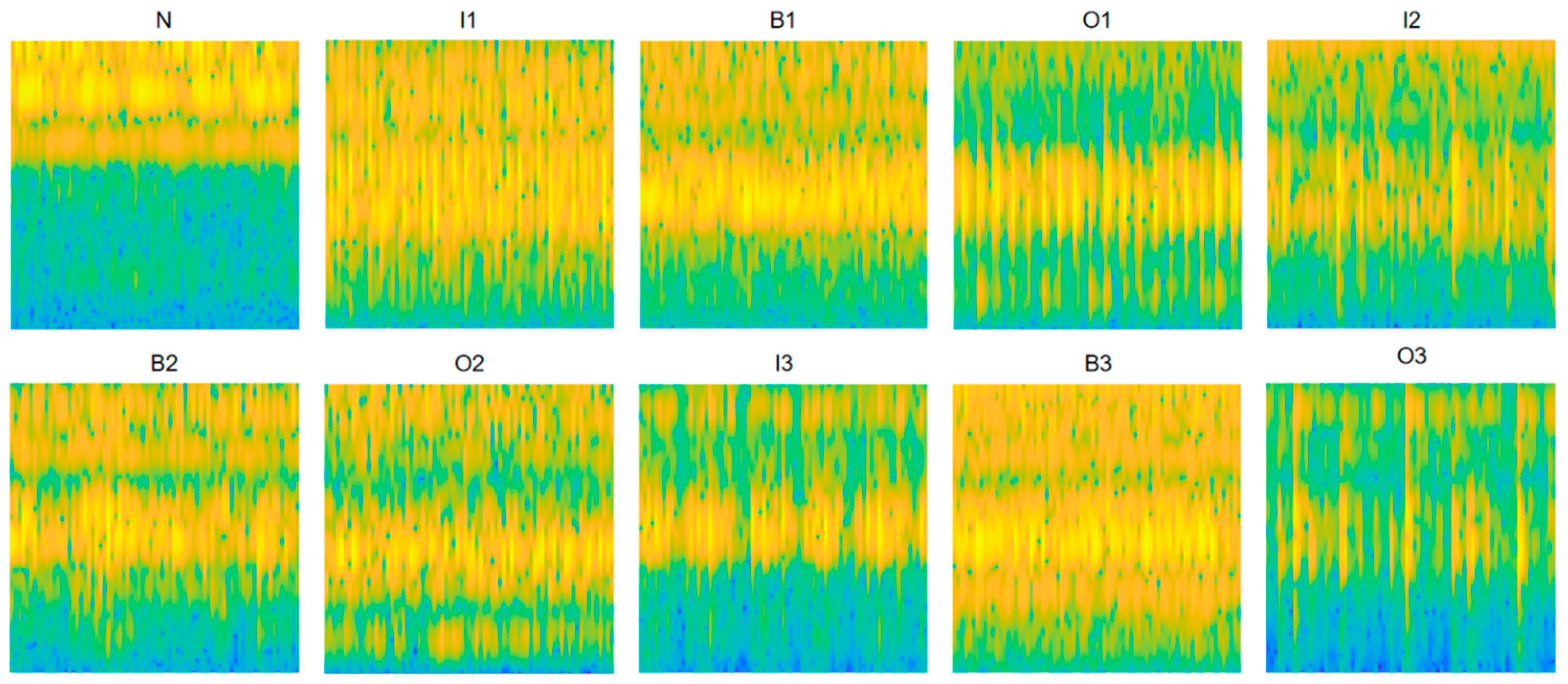
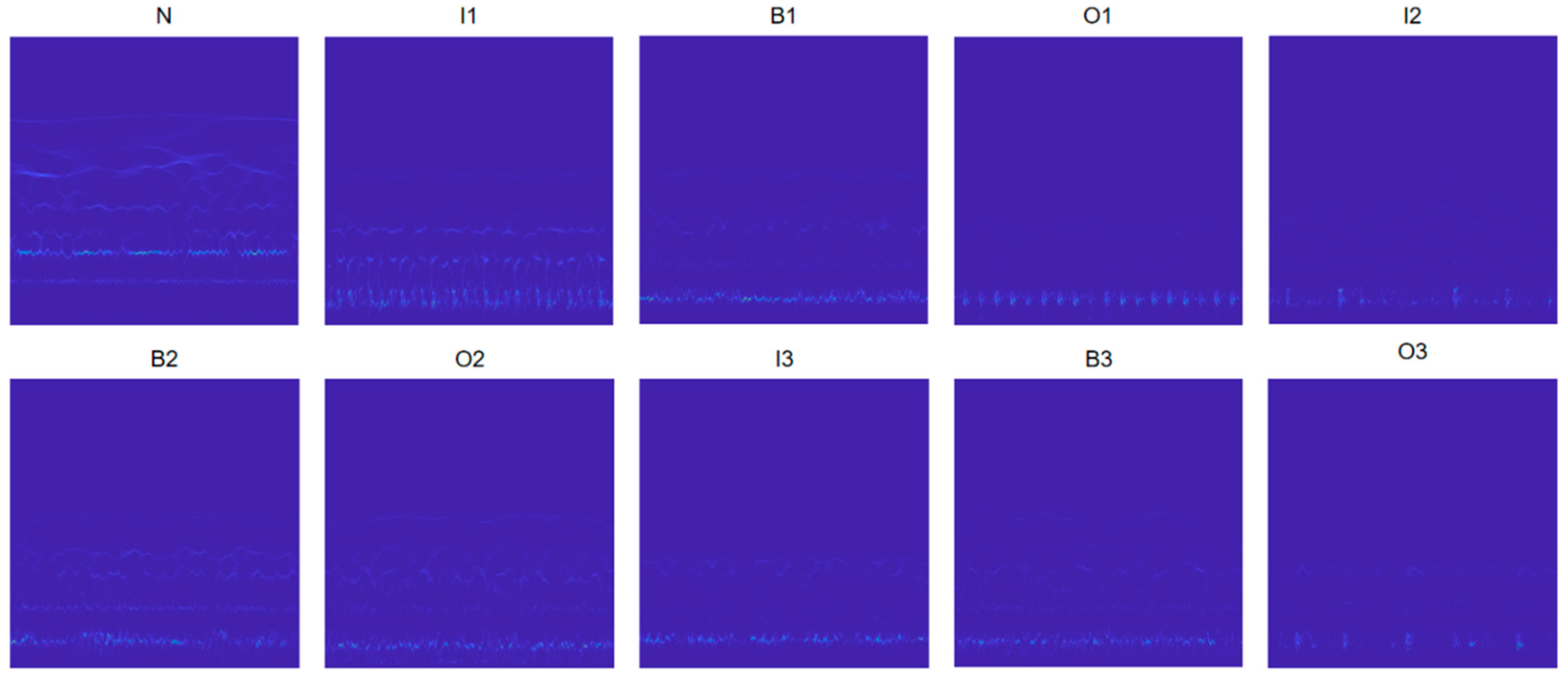
The sample set’s vibration signals undergo a short-time Fourier transform and a synchronized compressed wavelet transform, creating an image for each sample to form the feature sample set. This feature sample set is then randomly split into a training set and a test set based on a specified ratio.

(3)

A parallel CNN model is constructed and the model parameters are initialized.

(4)

The dual-channel parallel CNN training model processes both the training and test sets at the same time. During each iteration of training, the model is validated using the test set to monitor its convergence. After completing the necessary iterations and reaching convergence, the model is saved for future evaluation.

(5)

Once the training is complete, the model’s performance is assessed using the test set.

The troubleshooting flowchart in this paper is as follows:

Figure 6. Troubleshooting flowchart.

Figure 6. Troubleshooting flowchart.

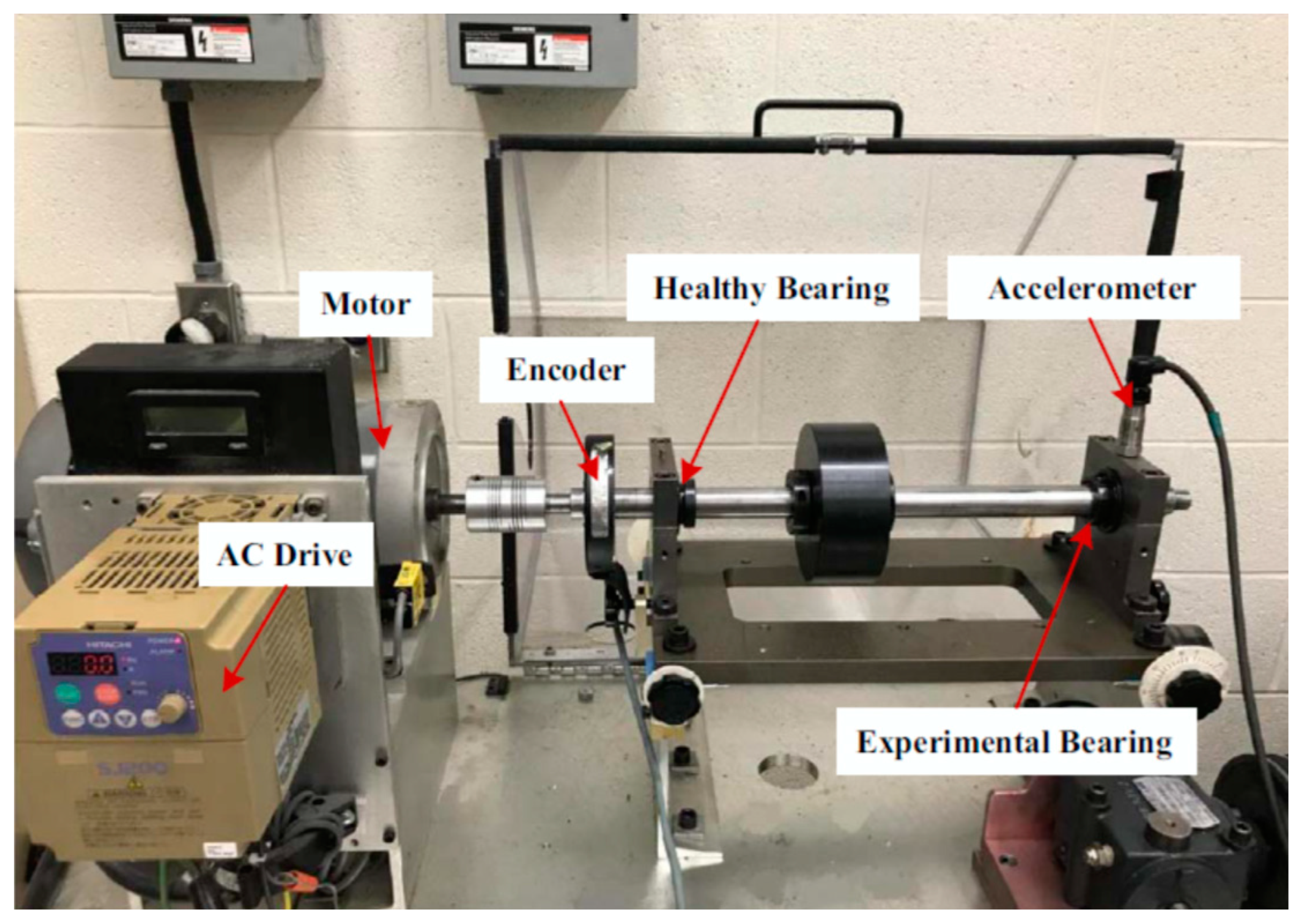
4. Experimental Section

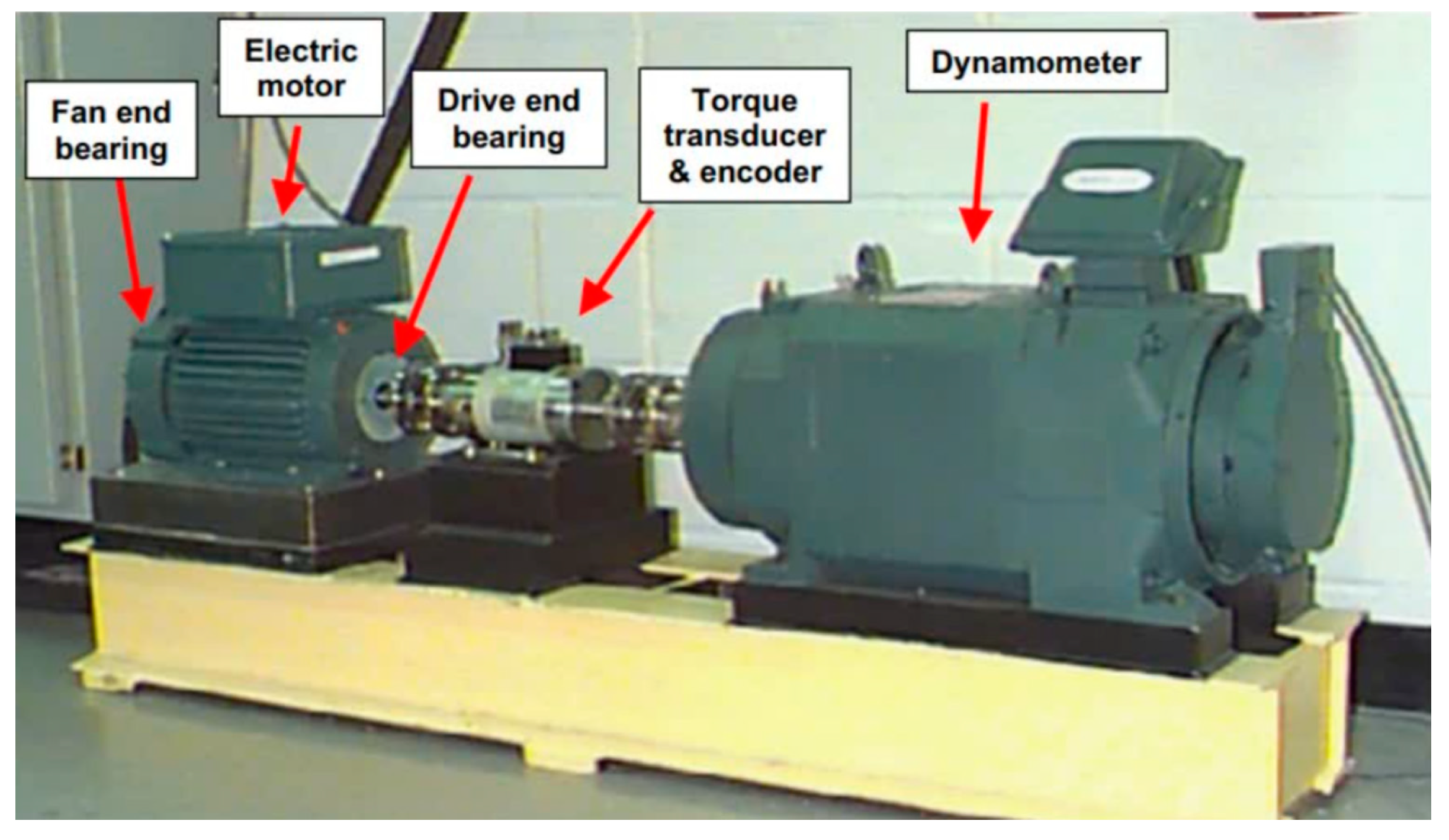
4.1. CWRU Dataset

To assess how well the proposed method performs, this study utilizes the CWRU bearing dataset provided by the Case Western Reserve University Bearing Data Center. This dataset is widely employed in the domain of failure diagnosis [41]. The experiments used drive-end bearing failure data, specifically the SKF 6205-2RS JEM deep groove ball bearing model. Failures were introduced by EDM technology and categorized based on damage location: inner ring, rolling element, and outer ring. Each location had three flaw sizes: 0.007 inch, 0.014 inch, and 0.021 inch. Vibration signals were collected under a 1 HP load at a sampling frequency of 12 kHz. In this study, we categorized the failures into 10 distinct groups. We set the sample length to 1024 and conducted 100 samples for each type of failure, totaling 1000 samples in the bearing failure diagnosis dataset. Their experimental platform is shown in Figure 7.

Table 1. CWRU dataset composition.

Fault Diameter/mm	Type of Fault	Fault Category	Sample Size
0	N	1	100
0.007	I1	2	100
0.014	I2	3	100
0.021	I3	4	100
0.007	B1	5	100
0.014	B2	6	100
0.021	B3	7	100
0.007	O1	8	100
0.014	O2	9	100
0.021	O3	10	100

provides a detailed breakdown of the dataset’s composition.

4.2. Data Generation and Model Training

4.2.1. Data Generation

By utilizing the previously gathered set of 1000 samples, both the short-time Fourier transform (STFT) and the synchronized compressed wavelet transform (SCWT) are employed. Each sample produces a corresponding STFT image and SCWT image, each with dimensions of 64 × 64 × 3. This results in a total of 1000 images for each transform. Figure 8 depicts the time–frequency plots produced by the short-time Fourier transform for various types of fault data related to bearing conditions. Meanwhile, Figure 9 shows the time–frequency diagrams generated by the synchronized compressed wavelet transform for the different fault data types of bearing conditions.

Figure 8 presents the data pertaining to each distinct bearing condition fault, as transformed by the short-time Fourier transform and represented in the time–frequency diagram. For example, Figure 8-N represents a normal signal in the bearing data, generated by the short-time Fourier transform and represented in a time–frequency diagram (in the data processing of normal signals, 100 different signal time–frequency diagrams are generated). Figure 8-I1 represents the bearing data with a value of 0. The damage to an inner-ring failure signal is 0.007 inches in size, as indicated by the short-time Fourier transform generated by the time–frequency diagram (Figure 8-I1). The damage to an inner-ring failure signal is 0.014 inches in size, as indicated by the short-time Fourier transform generated by the time–frequency diagram (Figure 8-I2). Figure 8-I2 depicts the time–frequency diagram generated by the short-time Fourier transform of an inner-ring fault signal with a damage size of 0.014 inches in the bearing data. Figure 8-I3 represents the time–frequency diagram generated by the short-time Fourier transform of an inner-ring fault signal with a damage size of 0.021 inches in the bearing data. Figure 8-B1 illustrates the time–frequency diagram generated by the short-time Fourier transform of a rolling-body fault signal with a damage size of 0.007 inches in the bearing data. Figure 8-B2 depicts the time–frequency diagram generated by the short-time Fourier transform of a rolling-body failure signal with a damage size of 0.014 inches in the bearing data. Figure 8-B3 presents the time–frequency diagram generated by the short-time Fourier transform of a rolling-body failure signal with a damage size of 0.021 inches in the bearing data. Figure 8-O1 illustrates the time–frequency diagram generated by the short-time Fourier transform of an outer-ring failure signal with a damage size of 0.007 inches in the bearing data. Figure 8-O1 depicts the damage size of 0.007 inches of an outer-ring fault signal, obtained through the short-time Fourier transform following the generation of the time–frequency diagrams. Figure 8-O2 illustrates the damage size of 0.014 inches of an outer-ring fault signal, also obtained through the short-time Fourier transform following the generation of the time–frequency diagrams. Figure 8-O3 represents the damage size of 0.021 inches of a failure of the outer-ring signal, obtained through the short-time Fourier transformation of the generated time–frequency diagrams. The N to O3 time–frequency diagram in Figure 9 has the same meaning as the N to O3 time–frequency diagram in Figure 8, with the exception that Figure 9 employs a synchronized compressed wavelet transform to process the bearing signal.

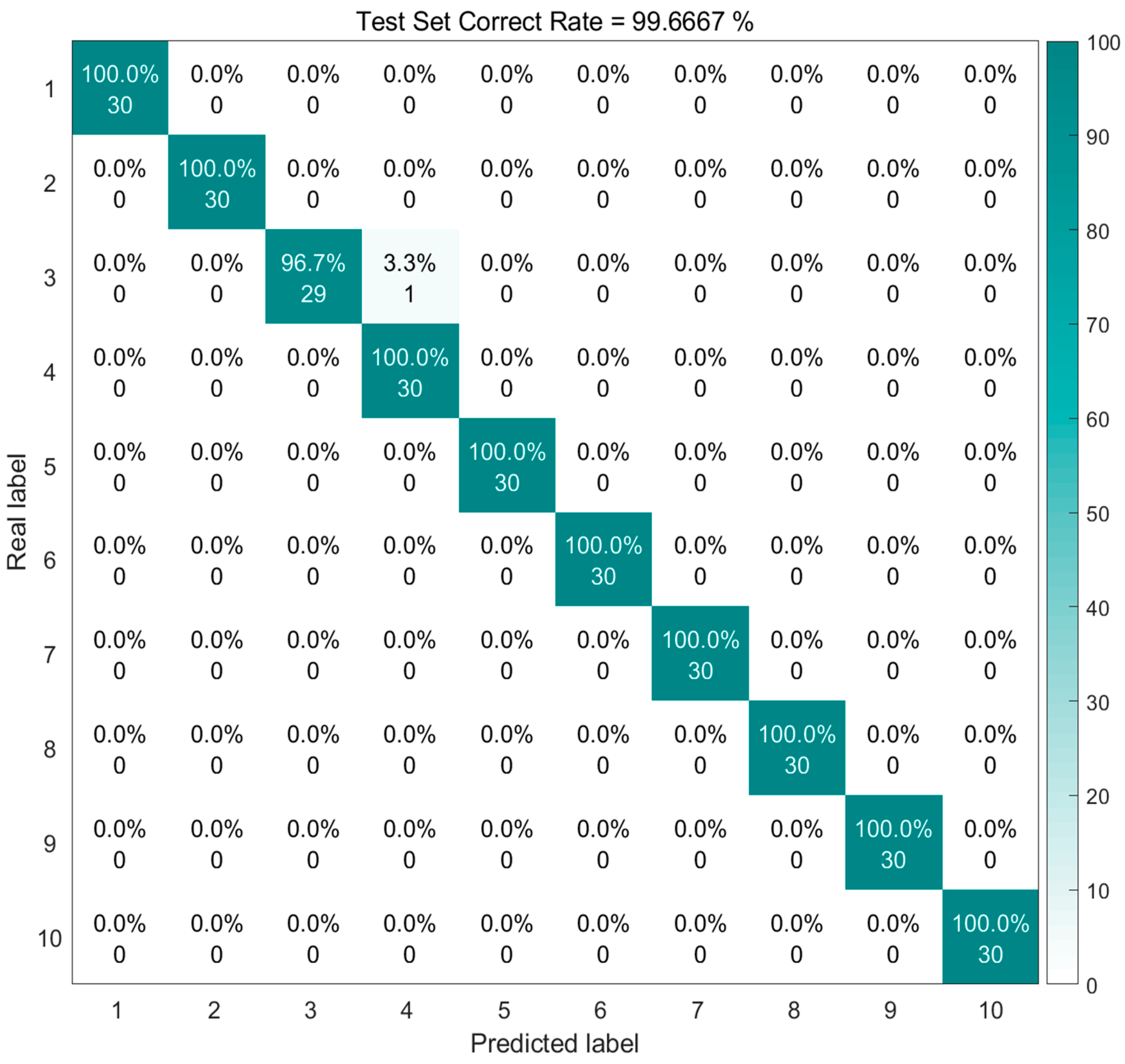
4.2.2. Model Training

In this paper, deep learning network models are constructed using MATLAB language with a computer configuration of 13th Gen Intel(R) Core(TM) i5-13400F 2.50 GHz, 16 GB RAM, and GTX 4060Ti 8 G GPU. A total of 1000 sets of samples are taken and randomly partitioned in the ratio of 7:3 into a training set, a test set, and no intersection between them.. The Adam optimizer is utilized for optimization, starting with a learning rate of 0.001. For the loss function, the cross-entropy function is employed. Training is conducted with a batch size of 256 over 250 iterations. The confusion matrix is illustrated in Figure 10.

In this paper, we enhance our assessment of the model’s fault diagnosis performance by examining its confusion matrix. This matrix is depicted in Figure 10, with the horizontal axis denoting the predicted category labels and the vertical axis showing the actual category labels. The values along the diagonal of the matrix indicate the count of samples accurately diagnosed for each fault category. Our analysis reveals that the proposed method encounters challenges in correctly predicting defects in category 3, specifically 0.014 mm inner-ring defects, while it exhibits improved diagnostic accuracy for several other categories.

To assess the feature extraction capability of the model, we conducted a feature visualization analysis of its output. The results are illustrated as follows: Figure 11a presents the initial distribution of data features, while Figure 11b depicts the visualization outcomes post-feature classification. When the parallel CNN processes fault signals, it transitions all 10 fault signal groups from their original chaotic state to a more organized aggregation. Although most signal points of different fault types are distinctly separated, a few points still overlap, and the spacing among major fault signal classes remains somewhat unclear. In contrast, Figure 11b reveals that the dual-stream CNN model effectively separates the fault signals, with clear distinctions between the different signal types and minimal distance between similar fault signal points. This indicates the parallel CNN model’s superior feature extraction performance in bearing fault diagnosis. The results of the feature visualization analysis are shown below:

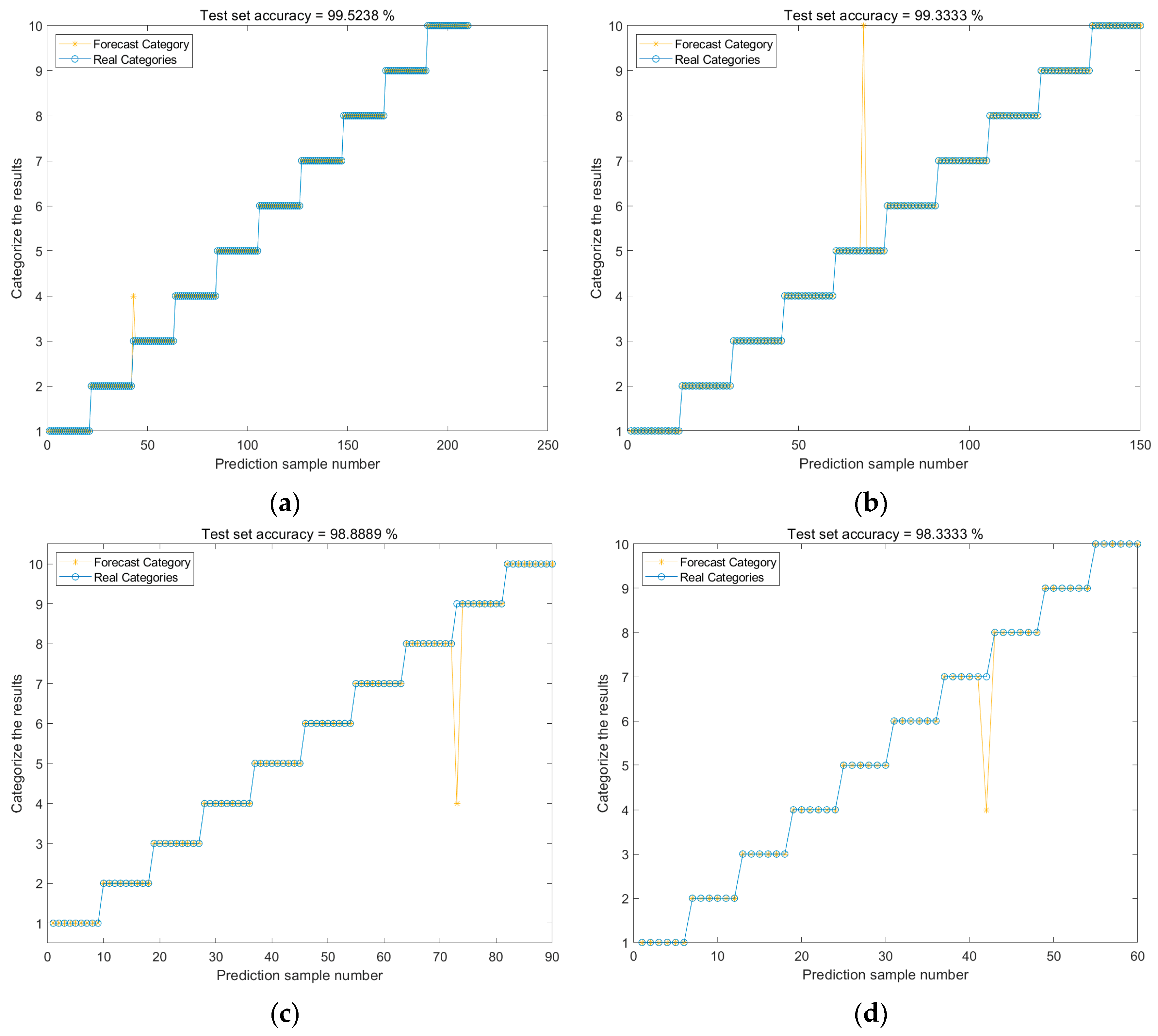
4.2.3. Fault Diagnosis with Different Sample Sizes

The author conducted comparative experiments with four different sample sizes and divided the training and testing sets into a 7:3 ratio.

The test results are shown in Figure 12.

Table 2. Model training results.

Experiment Number	Sample Size	Accuracy	F1 Score
1	700	99.52%	99.57%
2	500	99.33%	99.37%
3	300	98.89%	98.91%
4	200	98.33%	98.37%

below illustrates the diagnostic model’s accuracy with varying sample sizes drawn randomly from the original dataset for training. The table indicates a 0.56% accuracy difference between using 200 samples and 300 samples, a 0.44% difference between 300 samples and 500 samples, and a 0.19% difference between 500 samples and 700 samples. These findings suggest that the accuracy of the model shows minimal fluctuation with changes in the sample size, demonstrating the model’s stability.

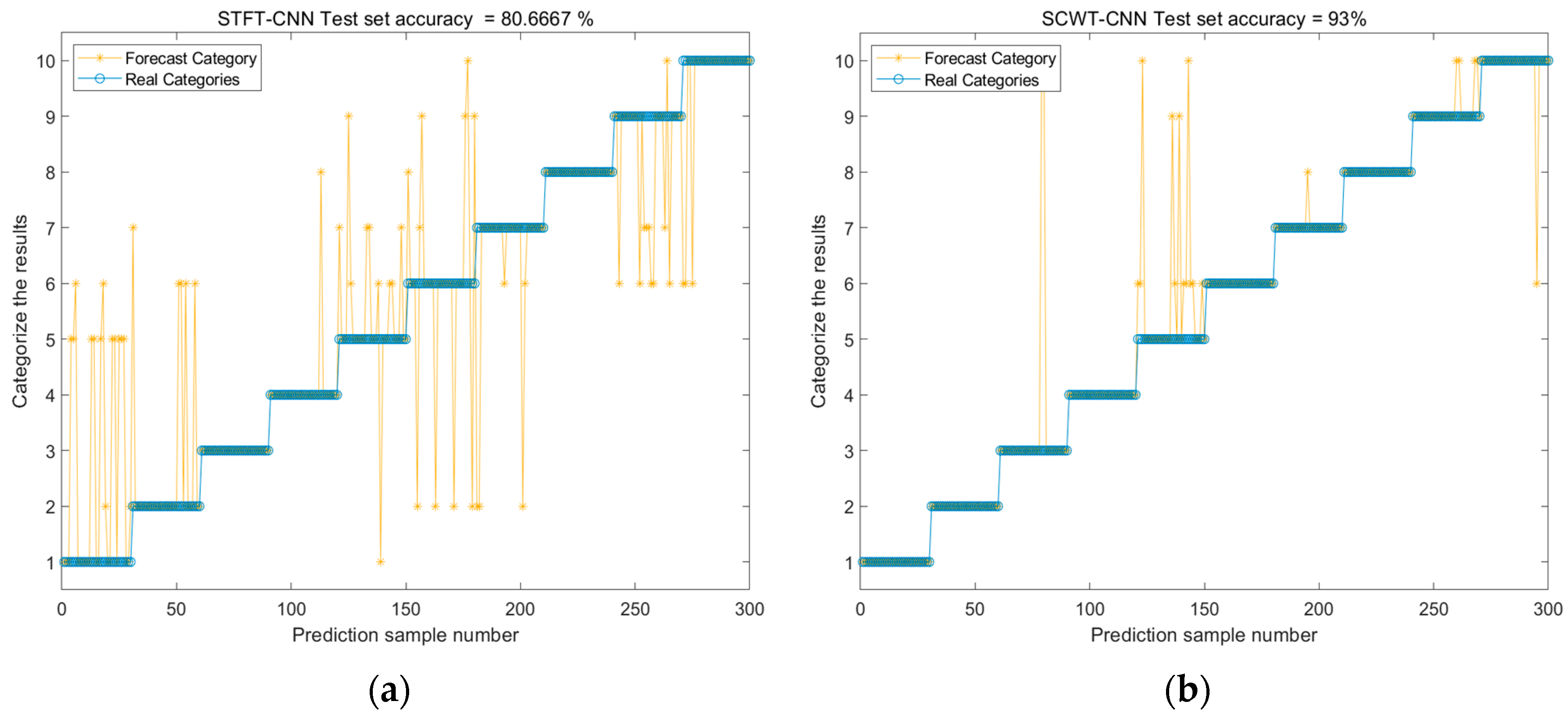
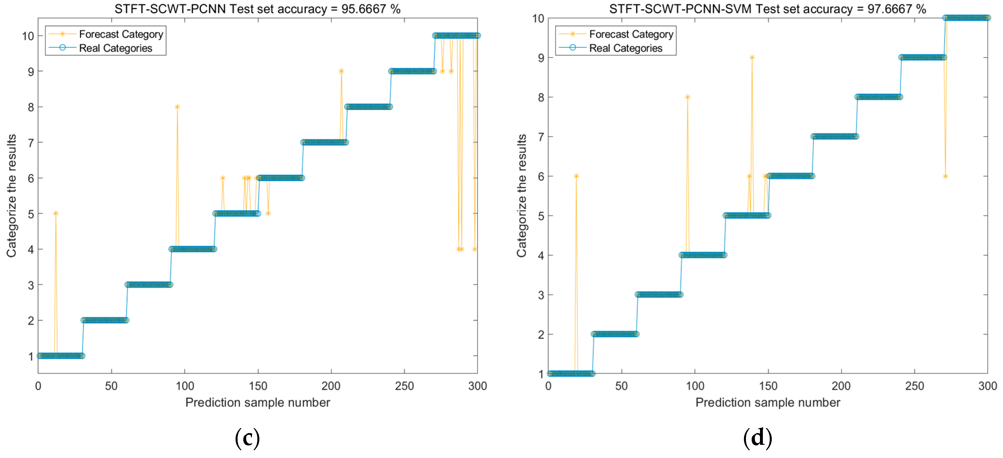
4.3. Advantages of Integrated Processing Methods and Parallel Networks

To further validate the advantages of hybrid signal processing method and parallel 2D-CNN in the bearing small-sample fault diagnosis method based on the hybrid signal processing method of SFTF and SCWT and parallel CNN proposed in this paper, respectively, all the parts related to SCWT in the corresponding models are removed, and only the STFT features are used to train the network; all the parts related to STFT are removed, and only the SCWT features are used to train the network; we use softmax for classification directly after CNN without SVM, removing parallel CNN and retaining SCWT, STFT, and SVM, where the SCWT + CNN method is that STFT performs the data processing, and CNN extracts the features and classifies them; the STFT + CNN method is that STFT performs the data processing and CNN extracts the features and classifies them; the SCWT + CNN + SVM method is that SCWT performs the data processing, CNN extracts the features and SVM performs the classification; the STFT + CNN + SVM method is that STFT performs the data processing, CNN extracts the features and SVM performs the classification; the SCWT + STFT + SVM method is that SCWT + STFT performs the data processing and SVM performs the classification; and the SCWT + STFT + parallel CNN method (the distinction between this method and the one described in the paper lies in the use of the softmax output layer for multi-category classification, as opposed to employing SVM processing) is to utilize SCWT + STFT to hybrid process the bearing vibration signals, generate new picture data, and parallel CNN to feature extract and classify the two, respectively.

Table 3. Diagnostic accuracy of different methods.

Mold	Treatment	Accuracy
CNN	SCWT	97.34%
CNN-SVM		98.00%
CNN	SFTF	94.28%
CNN-SVM		98.67%
SVM	SCWT-SFTF	85.63%
PCNN		98.67%
PCNN-SVM		99.34%

demonstrates that the hybrid signal processing method, which combines SCWT and STFT, consistently delivers superior accuracy compared to using either method individually. Notably, SCWT alone performs better than STFT alone. Nevertheless, the approach detailed in this paper offers even greater diagnostic accuracy than both the standalone SCWT and STFT methods. Additionally, integrating the SVM technique improves the accuracy of each individual signal processing method and similarly enhances the hybrid processing method’s performance. In conclusion, Table 3 indicates that the approach proposed in this study achieves the highest level of diagnostic accuracy.

4.4. Sample Size and Fault Diagnosis Accuracy Experiment

In order to demonstrate that the model can accomplish small sample fault diagnosis, a number of single-class samples 20, 30, 50, and 70 (a total of 200, 300, 500, and 700 samples) are imported into the six neural networks for training, and the fault diagnosis accuracies obtained by the six neural networks in different numbers of training samples are shown in

Table 4. Accuracy of training with different sample sizes.

Sample Size	SFTF-CNN	SCWT-CNN	SCWT-CNN-SVM	STFT-CNN-SVM	SCWT-SFTF-PCNN	SCWT-SFTF-PCNN-SVM
200	81.38%	82.5%	77.38%	81.86%	93.75%	98.43%
300	92.84%	94.57%	95.37%	93.71%	96.29%	98.57%
500	93.61%	96.60%	96.80%	98.67%	98.38%	98.67%
700	94.28%	97.34%	98.00%	98.67%	98.67%	99.34%

.

The diagnostic accuracies under four different numbers of samples are averaged to obtain the average diagnostic accuracy of each model as shown in

Table 5. UO dataset composition.

Bearing Condition	Operational State	Fault Category	Sample Size
Well-being	expedite	1	100
	decelerations	2	100
Inner-ring failure	expedite	3	100
	decelerations	4	100
Outer-ring failure	expedite	5	100
	decelerations	6	100
Ball fault	expedite	7	100
	decelerations	8	100
Composite fault	expedite	9	100
	decelerations	10	100

. In the case of the different numbers of samples of 700, 500, 300, and 200, the diagnostic accuracy of the methods in this paper is reduced by 0.77%, 0.10%, and 0.15%, respectively. At 300–200, the diagnostic accuracy of the SFTF-CNN and SCWT-CNN methods decreases too much, and the SCWT-SFTF-PCNN method decreases less compared with it, but the overall accuracy effect is still not as good as the method proposed in this paper. It shows that the diagnostic model designed in this paper still maintains a high diagnostic classification level when the number of samples is greatly reduced, which indicates that it can be a very good fault diagnosis method in small samples, and has good diagnostic robustness.

4.5. Exploring Generalizability

To assess the performance of the proposed model, we utilized a dataset provided by the University of Ottawa, Canada [42]. This dataset includes vibration signals from bearings exhibiting various health statuses under varying dynamic speeds. The bearings are categorized into four fault types based on their damage locations and operational conditions: inner ring, rolling element, outer ring, and a combined category (which encompasses inner-ring, outer-ring, and rolling element faults). Each fault type was evaluated under two distinct operational states: acceleration and deceleration. The vibration signals were collected with a load of 1 hp and sampled at a frequency of 200 kHz. For the analysis, we chose ramp-up and ramp-down sequences from bearings in healthy condition, as well as those with inner-ring, rolling element, outer-ring, and combined faults. Data preprocessing, following a method similar to that applied to the CWRU dataset, resulted in 1000 samples from the bearing fault diagnostic data. This dataset was then split into training and test sets, with a distribution of 70% for training and 30% for testing. The composition of the selected dataset is detailed in Table 5. Their experimental platform is shown in Figure 13.

Different diagnostic model accuracy comparison is carried out; the data processing methods and diagnostic models and Table 3 remain the same (the SVM method accuracy is too low and single STFT and SCWT + CNN + SVM enhancement is too small, so those three are not considered, and here, only STFT + CNN, STFT + CNN, STFT + SCWT + PCNN and the present method are the four kinds considered), and the results of the test are illustrated in Figure 14.

Figure 14 illustrates the application of all four methods in ten discrete scenarios, with 300 randomly selected samples utilized for each instance. In Figure 14a, problems are encountered in the first, second, fourth, fifth, sixth, seventh, ninth, and tenth categories and are more especially in the first category (acceleration bearing in a healthy state), fourth category (deceleration bearing in the inner-ring failure state), fifth category (acceleration bearing in the outer-ring failure state), and ninth category (acceleration bearing in the combined failure state), and finally the STFT+. The accuracy of CNN is 80.67% (this is because there is a lot of noise and interference in the bearings under the variable-speed operation environment, and STFT is sensitive to the noise, which interferes with the accuracy of the spectral analysis and reduces the accuracy of the model fault diagnosis). Problems were encountered in the third, fifth, seventh, ninth, and tenth categories in Figure 14b, but much fewer problems were encountered than in the STFT method, and the troubleshooting accuracy was improved by 12.33%, and finally, the SCWT + CNN had an accuracy of 93%. In Figure 14c, the first, fourth, fifth, sixth, seventh, and tenth categories encountered problems and were rare, with an accuracy of 95.67% for STFT + SCWT + PCNN. The method in this paper only encountered problems in the first, fourth, fifth, and ninth categories with a final accuracy of 97.67%. The experimental results show that the method of this paper is still applicable to other datasets with high robustness and can be well used for bearing fault diagnosis.

5. Conclusions

This paper presents a methodology for the diagnosis of bearing faults in small samples utilizing mixed signal processing techniques. The efficacy and benefits of the method are substantiated through a verification process using the CWRU bearing dataset. Furthermore, the robustness and applicability of the method on different datasets are confirmed by testing the variable-speed bearing dataset from the University of Ottawa, Canada. The experimental results demonstrate that the proposed model exhibits the highest diagnostic accuracy, reaching 98.43%, 98.57%, 98.67%, and 99.34%, respectively, in comparison to the existing network models with an equivalent number of small samples, particularly under variable-speed operating conditions. In this paper, a combined short-time Fourier transform (STFT) and synchronized compressed wavelet transform (SCWT) is proposed as a means of signal processing. This integrated method effectively employs both time-domain and frequency-domain data. The extraction of features from time–frequency images facilitates more efficient processing and enhances the visibility of image dominance. The SCWT’s multi-scale analysis capability enables the examination of the signal at diverse scales, thereby providing more comprehensive frequency information than the STFT. The integration of the STFT and the SCWT enhances the quality of the generated images and expands the depth of the attributes of the samples in the dataset. The model parameters and experimental results also serve as valuable data references for the existing fault diagnosis studies. It should be noted that only publicly available datasets were utilized in this study, whereas the actual operating environment of bearings typically encompasses a range of additional conditions, including noise and vibration. In future work, these different types of potential problems should be combined in order to create a more accurate model of actual operating conditions. Moreover, the integration of additional industrial failure datasets derived from real-world scenarios is essential for validating the composite failure types of weak and early failures, thereby enhancing the model’s practical utility.

References

1. Wu, G. Exploration of the safety management and maintenance of machinery manufacturing and processing equipment. J. Phys. Conf. Ser. 2021, 1885, 042047. [Google Scholar] [CrossRef]
2. Yani, I.; Resti, Y.; Burlian, F. Identification of bearing failure using signal vibrations. J. Phys. Conf. Ser. 2018, 1007, 012067. [Google Scholar] [CrossRef]
3. Firouzi, N.; Kazemi, S.R. Investigation on dynamic stability of Timoshenko beam using axial parametric excitation. Appl. Phys. A 2023, 129, 869. [Google Scholar] [CrossRef]
4. Simkulet, V.; Kočiško, M.; Hutyrová, Z.; Fečová, V. Analysis of the damage causes of high speed bearing failure. Appl. Mech. Mater. 2014, 616, 200–206. [Google Scholar] [CrossRef]
5. Khan, M.A.; Asad, B.; Kudelina, K.; Vaimann, T.; Kallaste, A. The bearing faults detection methods for electrical machines—The state of the art. Energies 2022, 16, 296. [Google Scholar] [CrossRef]
6. Zhang, X.; Zhao, B.; Lin, Y. Machine learning based bearing fault diagnosis using the case western reserve university data: A review. EEE Access 2021, 9, 155598–155608. [Google Scholar] [CrossRef]
7. Hu, L.; Wang, L.; Chen, Y.; Hu, N.; Jiang, Y. Bearing fault diagnosis using piecewise aggregate approximation and complete ensemble empirical mode decomposition with adaptive noise. Sensors 2022, 22, 6599. [Google Scholar] [CrossRef] [PubMed]
8. Barcelos, A.S.; Cardoso, A.J.M. Current-based bearing fault diagnosis using deep learning algorithms. Energies 2021, 14, 2509. [Google Scholar] [CrossRef]
9. Chan, H.P.; Hadjiiski, L.M.; Samala, R.K. Computer-aided diagnosis in the era of deep learning. Med. Phys. 2020, 47, e218–e227. [Google Scholar] [CrossRef]
10. Feng, J.; Yao, Y.; Lu, S.; Liu, Y. Domain knowledge-based deep-broad learning framework for fault diagnosis. IEEE Trans. Ind. Electron. 2020, 68, 3454–3464. [Google Scholar] [CrossRef]
11. Niu, G.; Wang, X.; Golda, M.; Mastro, S.; Zhang, B. An optimized adaptive PReLU-DBN for rolling element bearing fault diagnosis. Neurocomputing 2021, 445, 26–34. [Google Scholar] [CrossRef]
12. Lu, C.; Wang, Z.; Zhou, B. Intelligent fault diagnosis of rolling bearing using hierarchical convolutional network based health state classification. Adv. Eng. Inform. 2017, 32, 139–151. [Google Scholar] [CrossRef]
13. Qin, Y.; Shi, X. Fault diagnosis method for rolling bearings based on two-channel CNN under unbalanced datasets. Appl. Sci. 2022, 12, 8474. [Google Scholar] [CrossRef]
14. Li, J.; Liu, Y.; Li, Q. Intelligent fault diagnosis of rolling bearings under imbalanced data conditions using attention-based deep learning method. Measurement 2022, 189, 110500. [Google Scholar] [CrossRef]
15. Zhang, T.; Chen, J.; Li, F.; Zhang, K.; Lv, H.; He, S.; Xu, E. Intelligent fault diagnosis of machines with small & imbalanced data: A state-of-the-art review and possible extensions. ISA Trans. 2022, 119, 152–171. [Google Scholar]
16. Huang, Z.; Lei, Z.; Wen, G.; Huang, X.; Zhou, H.; Yan, R.; Chen, X. A multisource dense adaptation adversarial network for fault diagnosis of machinery. IEEE Trans. Ind. Electron. 2021, 69, 6298–6307. [Google Scholar] [CrossRef]
17. Hu, Y.; Liu, R.; Li, X.; Chen, D.; Hu, Q. Task-sequencing meta learning for intelligent few-shot fault diagnosis with limited data. IEEE Trans. Ind. Inform. 2021, 18, 3894–3904. [Google Scholar] [CrossRef]
18. Wang, Y.; Chen, L.; Liu, Y.; Gao, L. Wavelet-prototypical network based on fusion of time and frequency domain for fault diagnosis. Sensors 2021, 21, 1483. [Google Scholar] [CrossRef]
19. Altaf, M.; Akram, T.; Khan, M.A.; Iqbal, M.; Ch, M.M.I.; Hsu, C.-H. A new statistical features based approach for bearing fault diagnosis using vibration signals. Sensors 2022, 22, 2012. [Google Scholar] [CrossRef] [PubMed]
20. Pei, Z.; Jiang, H.; Li, X.; Zhang, J.; Liu, S. Data augmentation for rolling bearing fault diagnosis using an enhanced few-shot Wasserstein auto-encoder with meta-learning. Meas. Sci. Technol. 2021, 32, 084007. [Google Scholar] [CrossRef]
21. Gao, X.; Deng, F.; Yue, X. Data augmentation in fault diagnosis based on the Wasserstein generative adversarial network with gradient penalty. Neurocomputing 2019, 396, 487–494. [Google Scholar] [CrossRef]
22. Meng, Z.; Guo, X.; Pan, Z.; Sun, D.; Liu, S. Data segmentation and augmentation methods based on raw data using deep neural networks approach for rotating machinery fault diagnosis. IEEE Access 2019, 7, 79510–79522. [Google Scholar] [CrossRef]
23. Luo, J.; Huang, J.; Li, H. A case study of conditional deep convolutional generative adversarial networks in machine fault diagnosis. J. Intell. Manuf. 2020, 32, 407–425. [Google Scholar] [CrossRef]
24. Han, S.; Niu, P.; Luo, S.; Li, Y.; Zhen, D.; Feng, G.; Sun, S. A novel deep convolutional neural network combining global feature extraction and detailed feature extraction for bearing compound fault diagnosis. Sensors 2023, 23, 8060. [Google Scholar] [CrossRef] [PubMed]
25. Guo, Q.; Li, Y.; Liu, Y.; Gao, S.; Song, Y. Data augmentation for intelligent mechanical fault diagnosis based on local shared multiple-generator GAN. IEEE Sensors J. 2022, 22, 9598–9609. [Google Scholar] [CrossRef]
26. Tang, T.; Wu, J.; Chen, M. Lightweight model-based two-step fine-tuning for fault diagnosis with limited data. Meas. Sci. Technol. 2022, 33, 125112. [Google Scholar] [CrossRef]
27. Yin, H.; Li, Z.; Zuo, J.; Liu, H.; Yang, K.; Li, F. Wasserstein Generative Adversarial Network and Convolutional Neural Network (WG-CNN) for Bearing Fault Diagnosis. Math. Probl. Eng. 2020, 2020, 2604191. [Google Scholar] [CrossRef]
28. Manda, B.; Bhaskare, P.; Muthuganapathy, R. A convolutional neural network approach to the classification of engineering models. IEEE Access 2021, 9, 22711–22723. [Google Scholar] [CrossRef]
29. Zhang, T.; Liu, S.; Zhang, S. Review on Fault Diagnosis on the Rolling Bearing. J. Phys. Conf. Ser. 2021, 1820, 012107. [Google Scholar] [CrossRef]
30. Bapir, A.; Aydin, I. A comparative analysis of 1D convolutional neural networks for bearing fault diagnosis. In Proceedings of the 2022 International Conference on Decision Aid Sciences and Applications (DASA), Chiangrai, Thailand, 23–25 March 2022. [Google Scholar]
31. Schneider, A.P.; Paoletti, B.; Ottavy, X.; Brandstetter, C. Experimental monitoring of vibrations and the problem of amplitude quantification. J. Phys. Conf. Ser. 2023, 2511, 012017. [Google Scholar] [CrossRef]
32. Jain, S.; Salman, H.; Khaddaj, A.; Wong, E.; Park, S.M.; Mądry, A. A data-based perspective on transfer learning. In Proceedings of the IEEE/CVF Conference on Computer Vision and Pattern Recognition, Vancouver, BC, Canada, 17–24 June 2023. [Google Scholar]
33. Ferdowsi, A.; Saad, W. Brainstorming Generative Adversarial Networks (BGANs): Towards Multi-Agent Generative Models with Distributed Datasets. IEEE Internet Things J. 2023, 11, 7828–7840. [Google Scholar] [CrossRef]
34. Zheng, W.; Jin, M. Improving the performance of feature selection methods with low-sample-size data. Comput. J. 2022, 66, 1664–1686. [Google Scholar] [CrossRef]
35. Alvarez, R.; Borbor, E.; Grijalva, F. Comparison of methods for signal analysis in the time-frequency domain. In Proceedings of the 2019 IEEE Fourth Ecuador Technical Chapters Meeting (ETCM), Guayaquil, Ecuador, 13–15 November 2019. [Google Scholar]
36. Zielinski, T.P. Joint time-frequency resolution of signal analysis using Gabor transform. IEEE Trans. Instrum. Meas. 2001, 50, 1436–1444. [Google Scholar] [CrossRef]
37. Guo, J.; Wang, X.; Zhai, C.; Niu, J.; Lu, S. Fault diagnosis of wind turbine bearing using synchrosqueezing wavelet transform and order analysis. In Proceedings of the 2019 14th IEEE Conference on Industrial Electronics and Applications (ICIEA), Xi’an, China, 19–21 June 2019. [Google Scholar]
38. Zhang, J.H.; Sun, S.Y.; Zhu, X.L.; Zhou, Q.D.; Dai, H.W.; Lin, J.W. Diesel engine fault diagnosis based on an improved convolutional neural network. J. Vib. Shock 2022, 41, 139–146. [Google Scholar]
39. Liang, K.; Qin, N.; Huang, D.; Fu, Y. Convolutional Recurrent Neural Network for Fault Diagnosis of High-Speed Train Bogie. Complexity 2018, 2018, 4501952. [Google Scholar] [CrossRef]
40. Hu, P.; Zhao, C.; Huang, J.; Song, T. Intelligent and Small Samples Gear Fault Detection Based on Wavelet Analysis and Improved CNN. Processes 2023, 11, 2969. [Google Scholar] [CrossRef]
41. Smith, W.A.; Randall, R.B. Rolling element bearing diagnostics using the Case Western Reserve University data: A benchmark study. Mech. Syst. Signal Process. 2015, 64–65, 100–113. [Google Scholar] [CrossRef]
42. Sehri, M.; Dumond, P.; Bouchard, M. University of Ottawa constant load and speed rolling-element bearing vibration and acoustic fault signature datasets. Data Brief 2023, 49, 109327. [Google Scholar] [CrossRef]
Figure 1. Define a window function.
Symmetry 16 01178 g001
Figure 2. Adding windows to signals.
Symmetry 16 01178 g002
Figure 3. Hop size and overlap.
Symmetry 16 01178 g003
Figure 4. CNN structure diagram.
Symmetry 16 01178 g004
Figure 5. Dual-channel parallel CNN model with symmetry.
Symmetry 16 01178 g005
Figure 7. CWRU experimental device.
Symmetry 16 01178 g007
Figure 8. SFTF plot after short-time Fourier transform.
Symmetry 16 01178 g008
Figure 9. SCWT plot after synchronized compressed wavelet transform.
Symmetry 16 01178 g009
Figure 10. Confusion matrix.
Symmetry 16 01178 g010
Figure 11. Feature visualization map. (a) Distribution of raw data features; (b) visualization after feature classification.
Symmetry 16 01178 g011
Figure 12. Comparison of test results for different sample data. (a) Test results with 700 sample size; (b) test results with 500 sample size; (c) test results with 300 sample size; (d) test results with 200 sample size.
Symmetry 16 01178 g012
Figure 13. UO experimental device.
Symmetry 16 01178 g013
Figure 14. Test results: (a) STFT + CNN test results; (b) SCWT + CNN test results; (c) STFT + SCWT + PCNN test results; (d) test results of this method.
Symmetry 16 01178 g014aSymmetry 16 01178 g014b