Abstract
The novelty and main contributions of this paper are reflected in four aspects. First, we introduce multi-fractional phasor in Theorem 1. Second, we propose the motion phasor equations of seven types of multi-fractional vibrators in Theorems 2, 12, 22, 32, 43, 54, and 65, respectively. Third, we present the analytical expressions of response phasors of seven types of multi-fractional vibrators in Theorems 10, 20, 30, 41, 52, 63, and 74, respectively. Fourth, we bring forward the analytical expressions of stationary sinusoidal responses of seven types of multi-fractional vibrators in Theorems 11, 21, 31, 42, 53, 64, and 75, respectively. In addition, by using multi-fractional phasor, we put forward the analytical expressions of vibration parameters (equivalent mass, equivalent damping, equivalent stiffness, equivalent damping ratio, equivalent damping free natural angular frequency, equivalent damped natural angular frequency, equivalent frequency ratio) and frequency transfer functions of seven types of multi-fractional vibrators. Demonstrations exhibit that the effects of multi-fractional orders on stationary sinusoidal responses of those multi-fractional vibrators are considerable.
1. Introduction
The topic of fractional vibrations remains hot, see, e.g., Uchaikin ([], Chap. 7), Duan [], Duan et al. [,], Pskhu and Rekhviashvili [], Zelenev et al. [], Freundlich [,], Al-rabtah et al. [], Zurigat [], Blaszczyk [], Blaszczyk and Ciesielski [], Blaszczyk et al. [], Achar et al. [,,]), Rossikhin and Shitikova [,,,], Rossikhin [], Shitikova [,,], Shitikova et al. [], El-Nabulsi and Anukool [], Liu et al. [], Sofi [], Li [,,], simply mentioning a few.
There are three research shortcomings in the field of fractional vibrations. The first is that research works, such as those on the responses of fractional vibrations, are usually in numerical computations, see, e.g., [,,,,,,,,,,,,,,,,,,,,,,,,,,,,,,,,,,,,,,,,,,,,,,,,,,,,,,,], to mention a few. The analytical expressions are rarely reported, with the author’s previous work being among the few to report on these expressions [,,]. The second is that reports regarding the multi-fractional vibrators in the forms of (1)–(7) below
are seldom seen, where α(ω), β(ω), and λ(ω) are varying orders in terms of vibration frequency ω, either deterministically or randomly. In fact, reports regarding (3)–(7) are rarely seen even in the case of α(ω), or β(ω), or λ(ω) being constant. The third is the lack of studies that investigate stationary responses to sinusoidal excitations using fractional phasor. Note that the author’s previous work [] did not consider the seventh type of multi-fractional vibrators (7). In addition, it did not report the stationary sinusoidal responses of (1)–(7) either. This paper aims at filling up the mentioned research gaps by bringing forward the analytical expressions of stationary sinusoidal responses of seven types of multi-fractional vibration systems (1)–(7) methodologically using multi-fractional phasor, as newly introduced in this research.
The rest of the paper is organized as follows. In Section 2, we describe the fractional phasor and introduce the multi-fractional phasor. We present the analytic expressions of the results (equivalent motion phasor equations, equivalent masses, equivalent dampings, equivalent stiffnesses, equivalent damping ratios, equivalent damping free natural angular frequencies, equivalent damped natural angular frequencies, equivalent frequency ratios, frequency transfer functions, response phasors, and stationary sinusoidal responses) of seven types of multi-fractional vibrators in Section 3, Section 4, Section 5, Section 6, Section 7, Section 8 and Section 9, respectively. Discussions are provided in Section 10, followed by concluding remarks and a summary.
2. Multi-Fractional Phasor
Steinmetz introduced the theory and method of phasor in electrical engineering [,,]. Den Hartog’s work [] may be an early literature applying the phasor method to deal with stationary responses to sinusoidal excitations in vibrations. It is now a widely used method in vibrations (Jin and Xia [], Harris [], Nakagawa and Ringo [], Palley et al. [], Grote and Antonsson [], Allemang and Avitabile [], Soong and Grigoriu [], Rothbart and Brown []).
When f(t) = F0sin(ωt + θ), with the Euler formula, we write f(t) = Im{F0exp[i(ωt + θ)]}. Denote the phasor of f(t) by F. It is given by
Therefore, one can write
Let n be a positive integer. Then, by using phasor,
F = F0exp(iθ).
f(t) = Im[Fexp(iωt)].
f(n)(t) = (iω)nIm[Fexp(iωt)].
When a vibration system is driven by a sinusoidal excitation below
we can change the above differential equation to an algebraic one in the form
where X is the phasor of response x(t) in the form
Denote by H(ω) the frequency transfer function. It is in the form
Using the damping ratio and frequency ratio where H(ω)
can be written by
Using the polar system, we have
where
Therefore, the response x(t) is given by
Mx″(t) + cx′(t) + kx(t) = F0sin(ωt + θ),
(iω)2mX + (iω)cX + kX = F,
x(t) = Im[Xexp(iωt)] = |H(ω)|F0sin(ωt + θ − φ).
Equation (18) expresses the stationary sinusoidal solution to the second-order differential Equation (11). It is algebraically derived using the phasor method. In order to deal with stationary sinusoidal solution to a fractional vibrator using the tool of phasor, fractional phasor is necessary. Further, when dealing with stationary sinusoidal solution to a multi-fractional vibrator using the method of phasor, multi-fractional phasor is essential. We express fractional phasor and multi-fractional one in Lemma 1 and Theorem 1 below, respectively.
Lemma 1 (Fractional phasor).
Suppose that y(t) = Y0sin(ωt + θ). Let Y be the phasor of y(t). It is in the form of Y = Y0exp(iθ). The phasor of y(v)(t) (v ≥ 0) is given by (iω)vY.
Proof.
Since y(v)(t) = Im{(iω)vY0exp[i(ωt + θ)]} = Im[(iω)vYexp(iωt)], the phasor of y(v)(t) is (iω)vY. Lemma 1 holds. The proof is finished. □
Theorem 1 (Multi-fractional phasor).
Suppose that y(t) = Y0sin(ωt + θ). Denote by Y the phasor of y(t). It is in the form of Y = Y0exp(iθ). The phasor of (v ≥ 0) is given by
Proof.
Using the Euler formula to express y(t) produces y(t) = Im{Y0exp[i(ωt + θ)]} = Im[Yexp(iωt)]. Thus, Hence, Theorem 1 holds. The proof is finished. □
Note that the concept of fractional phasor and its expression can be seen in the field of electronic and electrical engineering, see, e.g., Zhang and Shu [], Sarafraz and Tavazoei [,], Jia et al. [], Shamim et al. [], Malek et al. [], Zhao et al. [], Adhikary et al. [], to mention a few. However, the reports regarding the concept and expression of multi-fractional phasor are rarely seen. Therefore, we use the term lemma to describe the fractional phasor (Lemma 1) since it is a known result and the terminology theorem to express the multi-fractional phasor (Theorem 1) because it is newly introduced in this paper.
3. Results Regarding Multi-Fractional Vibrators of Type 1
In this Section, with respect to multi-fractional vibrators of type 1, we address the motion phasor equation in Section 3.1, the expressions of equivalent vibration parameters in Section 3.2, the expression of frequency transfer function in Section 3.3, and the expressions of stationary sinusoidal responses, respectively, in phasor and time to a type 1 multi-fractional vibrator in Section 3.4.
3.1. Motion Phasor Equation of Type 1 Multi-Fractional Vibrator
Theorem 2 (Motion phasor equation 1).
The motion phasor equation of a type 1 multi-fractional vibrator is expressed by
where X1 is the phasor of response x1(t) and F is the phasor of excitation f(t) = F0sin(ωt + θ).
Proof.
Expressing both sides of using phasor results in (19). This finishes the proof. □
Consider the principal branch of The left side of (19) can be expressed by
Writing the right side of the above by
we express the motion phasor equation of a type 1 multi-fractional vibrator by
Note that implies fractional inertia force. Hence, 1 < α(ω) < 3.
3.2. Equivalent Parameters of Type 1 Multi-Fractional Vibrator
The equivalent vibration parameters for a type 1 multi-fractional vibrator include equivalent mass, equivalent damping, equivalent damping ratio, equivalent damping free natural angular frequency, equivalent damped natural angular frequency, and equivalent frequency ratio.
3.2.1. Equivalent Mass of Type 1 Multi-Fractional Vibrator
Theorem 3 (Equivalent mass 1).
Let meq1 be the equivalent mass of a multi-fractional vibrator of type 1. Then,
Proof.
From the right side of (22), we have
In the above, meq1 is the equivalent mass for a multi-fractional vibrator of type 1. This finishes the proof. □
Figure 1 indicates some plots of meq1.
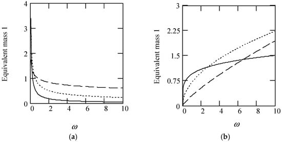
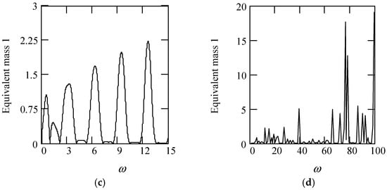
Figure 1.
Plots of meq1 for m = 1. (a). meq1 for α(ω) = 1.2 (solid), 1.5 (dot), 1.8 (dash). (b). meq1 when α(ω) = 2.2 (solid), 2.5 (dot), 2.8 (dash). (c). meq1 when α(ω) = 1.4 + cos(2ω). (d). meq1 when α(ω) is a uniformly distributed random function with the range (0.3, 2.7).
3.2.2. Equivalent Damping of Type 1 Multi-Fractional Vibrator
Theorem 4 (Equivalent damping 1).
Let ceq1 be the equivalent damping of a multi-fractional vibrator of type 1. Then,
Proof.
From the second item on the right side of (24), we see that (25) is true. The proof is finished. □
Some plots of ceq1 are indicated in Figure 2.
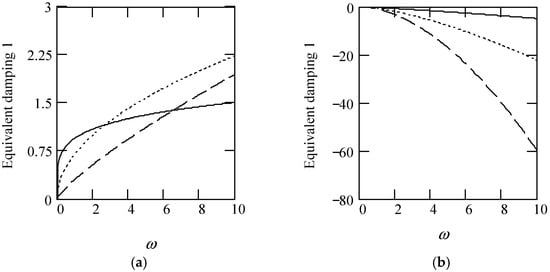
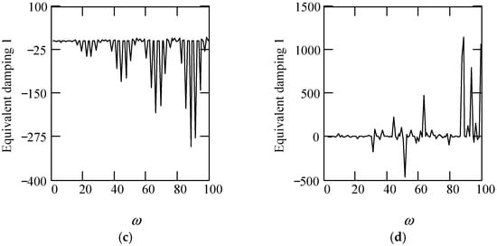
Figure 2.
Plots of ceq1 for m = 1. (a). ceq1 when α(ω) = 1.2 (solid), 1.5 (dot), 1.8 (dash). (b). ceq1 when α(ω) = 2.2 (solid), 2.5 (dot), 2.8 (dash). (c). ceq1 for α(ω) = 1.4 + cos(2ω). (d). ceq1 when α(ω) is a uniformly distributed random function with the range (0.3, 2.7).
3.2.3. Equivalent Damping Ratio of Type 1 Multi-Fractional Vibrator
Denote by ζeq1 the equivalent damping ratio of a multi-fractional vibrator of type 1. Define it by
Theorem 5 (Equivalent damping ratio 1).
The expression of ζeq1 is given by
Proof.
Substituting meq1 and ceq1 into (26) yields (27). The proof is finished. □
Figure 3 illustrates some plots of ζeq1.
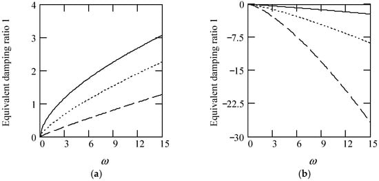
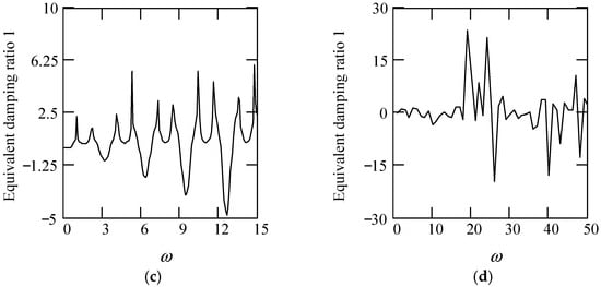
Figure 3.
Plots of ζeq1 for m = 1. (a). ζeq1 for α(ω) = 1.2 (solid), 1.5 (dot), 1.8 (dash). (b). ζeq1 when α(ω) = 2.2 (solid), 2.5 (dot), 2.8 (dash). (c). ζeq1 for α(ω) = 1.4 + cos(2ω). (d). ζeq1 when α(ω) is a uniformly distributed random function with the range (0.3, 2.7).
3.2.4. Equivalent Damping Free Natural Angular Frequency of Type 1 Multi-Fractional Vibrator
Introduce a term of equivalent damping free natural angular frequency. Let it be ωeqn1. Define it by
Theorem 6 (Equivalent damping free natural angular frequency 1).
The quantity ωeqn1 is given by
Proof.
Substituting meq1 into (28) produces (29). The proof is finished. □
Some plots of ωeqn1 are shown in Figure 4.
Figure 4.
Plots of ωeqn1 for m = 1 and k = 1. (a). ωeqn1 when α(ω) = 1.2 (solid), 1.5 (dot), 1.8 (dash). (b). ωeqn1 for α(ω) = 2.2 (solid), 2.5 (dot), 2.8 (dash). (c). ωeqn1 for α(ω) = 1.4 + cos(2ω). (d). ωeqn1 when α(ω) is a uniformly distributed random function with the range (0.3, 2.7).
3.2.5. Equivalent Damped Natural Angular Frequency of Type 1 Multi-Fractional Vibrator
Without losing the generality in vibration engineering, we only consider |ζeq1| ≤ 1 in what follows. Let ωeqd1 be the equivalent damped natural frequency of a type 1 multi-fractional vibrator. Define it by
Theorem 7 (Equivalent damped natural angular frequency 1).
The quantity ωeqd1 is expressed by
Proof.
Substituting ζeq1 and ωeqn1 into (30) yields (31). This finishes the proof. □
Some plots of ωeqd1 are indicated in Figure 5.
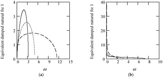
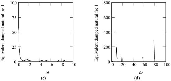
Figure 5.
Illustrations of ωeqd1 for m = 1 and k = 1. (a). ωeqd1 when α(ω) = 1.3 (solid), 1.5 (dot), 1.8 (dash). (b). ωeqd1 for α(ω) = 2.2 (solid), 2.4 (dot), 2.6 (dash). (c). ωeqd1 for α(ω) = 1.4 + cos(2ω). (d). ωeqd1 when α(ω) is a uniformly distributed random function with the range (0.3, 2.7).
3.2.6. Equivalent Frequency Ratio of Type 1 Multi-Fractional Vibrator
Let γeq1 be the equivalent frequency ratio of a multi-fractional vibrator of type 1. Define it by
Theorem 8 (Equivalent frequency ratio 1).
The quantity γeq1 is in the form
Proof.
Substituting ωeqn1 into (32) produces (33). The proof is finished. □
Some plots of γeq1 are shown in Figure 6.
Figure 6.
Illustrations of γeq1 for m = 1 and k = 1. (a). γeq1 when α(ω) = 1.2 (solid), 1.5 (dot), 1.8 (dash). (b). γeq1 for α(ω) = 2.2 (solid), 2.5 (dot), 2.8 (dash). (c). γeq1 for α(ω) = 1.4 + cos(2ω). (d). γeq1 when α(ω) is a uniformly distributed random function with the range (0.3, 2.7).
3.3. Frequency Transfer Function of Type 1 Multi-Fractional Vibrator
Theorem 9 (Frequency transfer function 1).
Denote by H1(ω) the frequency transfer function of a type 1 multi-fractional vibrator in phasor. Then,
Proof.
Considering the motion phasor equation in the form
we have (34). The proof is finished. □
Write the motion phasor equation by
Using γeq1, we can write H1(ω) by
The amplitude of H1(ω) is given by
Or
The phase of H1(ω) is in the form
Or
Or
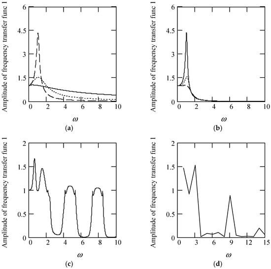
Figure 7.
Illustrations of |H1(ω)| for m = 1 and k = 1. (a). |H1(ω)| when α(ω) = 1.2 (solid), 1.5 (dot), 1.8 (dash). (b). |H1(ω)| for α(ω) = 2.2 (solid), 2.5 (dot), 2.8 (dash). (c). |H1(ω)| for α(ω) = 1.4 + cos(2ω). (d). |H1(ω)| when α(ω) is a uniformly distributed random function with the range (0.3, 2.7).
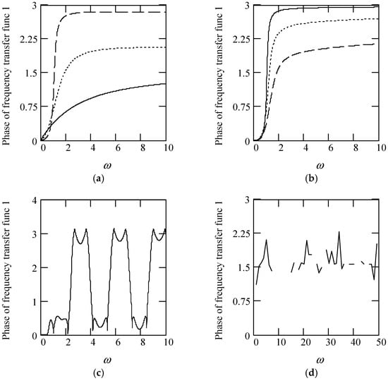
Figure 8.
Illustrations of φ1(ω) for m = 1 and k = 1. (a). φ1(ω) when α(ω) = 1.2 (solid), 1.5 (dot), 1.8 (dash). (b). φ1(ω) for α(ω) = 2.2 (solid), 2.5 (dot), 2.8 (dash). (c). φ1(ω) for α(ω) = 1.4 + cos(2ω). (d). φ1(ω) when α(ω) is a uniformly distributed random function with the range (0.3, 2.7).
3.4. Stationary Response to Sinusoidal Vibration of Type 1 Multi-Fractional Vibrator
There are two expressions of stationary sinusoidal response to a type 1 multi-fractional vibrator. One is the expression in the phasor domain and the other in the time domain. We explain them in Theorems 10 and 11, respectively.
Theorem 10 (Response phasor 1).
The response phasor of a type 1 multi-fractional vibrator is expressed by
Proof.
Writing X1 = H1(ω)F yields the above. The proof is finished. □
Equivalently, X1 can be written by
Theorem 11 (Stationary sinusoidal response 1).
The stationary sinusoidal response to a type 1 multi-fractional vibrator is expressed by
Proof.
Note that = Im[X1exp(iωt)]. As X1 = H1(ω)F = H1(ω)F0exp(iθ), we have the above. The proof is finished. □
Figure 9 and Figure 10 indicate some illustrations of x1(t), exhibiting that there is a significant effect of fractional order α(ω) on the sinusoidal response x1(t).
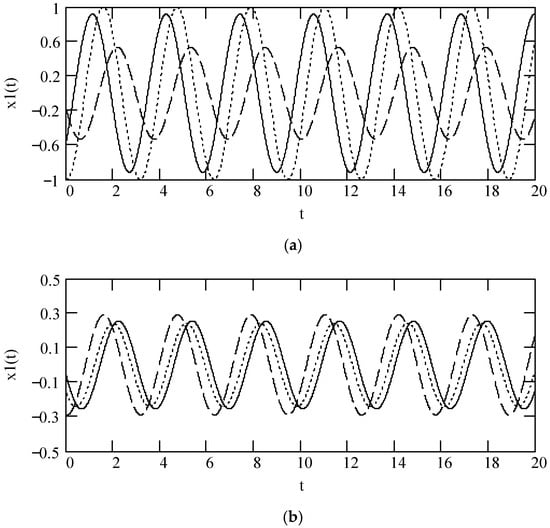
Figure 9.
Illustrations of x1(t) for ω = 2, F0 = 1, θ = 0, m = 1, and k = 1. (a). x1(t) when α(ω) = 1.2 (solid), 1.5 (dot), 1.8 (dash). (b). x1(t) for α(ω) = 2.2 (solid), 2.5 (dot), 2.8 (dash).
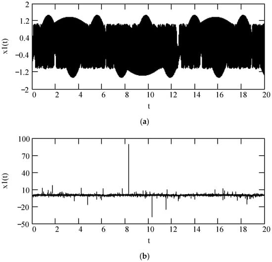
Figure 10.
Illustrations of x1(t) for F0 = 1, θ = 0, m = 1, and k = 1. (a). x1(t) when for α(ω) = 1.4 + cos(2ω). (b). x1(t) when α(ω) is a uniformly distributed random function with the range (0.3, 2.7).
4. Results in Multi-Fractional Vibrators of Type 2
We explain the results of type 2 multi-fractional vibrators in this Section as follows. The motion phasor equation is described in Section 4.1, the expressions of equivalent vibration parameters are discussed in Section 4.2, the expression of frequency transfer function is represented in Section 4.3, and the expressions of stationary sinusoidal response to a type 2 multi-fractional vibrator are expressed in Section 4.4.
4.1. Motion Phasor Equation of Type 2 Multi-Fractional Vibrator
Theorem 12 (Motion phasor equation 2).
Let X2 be the phasor of response x2(t) of a type 2 multi-fractional vibrator. Let F be the phasor of excitation f(t) = F0sin(ωt + θ). Then, the motion phasor equation of a type 2 multi-fractional vibrator is expressed by
Proof.
Using phasor to express both sides of yields (46). This completes the proof. □
Taking into account the principal branch of we write the left side of (46) by
Writing the right side of the above by
produces the motion phasor equation of a type 2 multi-fractional vibrator in the form
Note that designates a fractional damping force. Consequently, 0 < β(ω) < 2.
4.2. Equivalent Parameters of Type 2 Multi-Fractional Vibrator
The equivalent vibration parameters described in this Subsection for a type 2 multi-fractional vibrator contain equivalent mass, equivalent damping, equivalent damping ratio, equivalent damping free natural angular frequency, equivalent damped natural angular frequency, and equivalent frequency ratio.
4.2.1. Equivalent Mass of Type 2 Multi-Fractional Vibrator
Theorem 13 (Equivalent mass 2).
Let meq2 be the equivalent mass of a multi-fractional vibrator of type 2. Then,
Proof.
Considering the first item on the right side of (49), we see that the above is true. This finishes the proof. □
Figure 11 shows some of the plots of meq2.
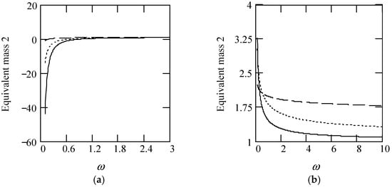
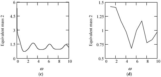
Figure 11.
Plots of meq2 for m = 1 and c = 1. (a). meq2 for β(ω) = 0.3 (solid), 0.6 (dot), 0.9 (dash). (b). meq2 when β(ω) = 1.3 (solid), 1.6 (dot), 1.9 (dash). (c). meq2 when β(ω) = 1.2 + 0.5cos(2ω). (d). meq2 when β(ω) is a uniformly distributed random function with the range (0.3, 1.7).
4.2.2. Equivalent Damping of Type 2 Multi-Fractional Vibrator
Theorem 14 (Equivalent damping 2).
Let ceq2 be the equivalent damping of a multi-fractional vibrator of type 2. Then,
Proof.
From the second item on the right side of (49), we see that the above holds. The proof is finished. □
Figure 12 illustrates some plots of ceq2.
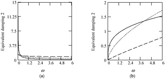
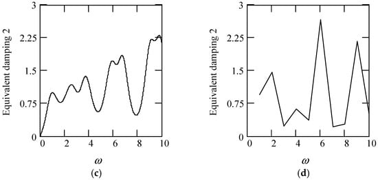
Figure 12.
Plots of ceq2 for c = 1. (a). ceq2 for β(ω) = 0.3 (solid), 0.6 (dot), 0.9 (dash). (b). ceq2 when β(ω) = 1.3 (solid), 1.6 (dot), 1.9 (dash). (c). ceq2 when β(ω) = 1.2 + 0.5cos(2ω). (d). ceq2 when β(ω) is a uniformly distributed random function with the range (0.3, 1.7).
4.2.3. Equivalent Damping Ratio of Type 2 Multi-Fractional Vibrator
Theorem 15 (Equivalent damping ratio 2).
Let ζeq2 be the equivalent damping ratio of a multi-fractional vibrator of type 2. Define it by
Then,
where is the primary damping ratio.
Proof.
Substituting meq2 and ceq2 into (52) results in (53). The proof is finished. □
Figure 13 shows some plots of ζeq2.
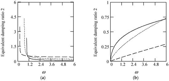
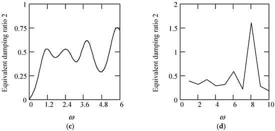
Figure 13.
Plots of ζeq2 for m = 1 and c = 1, and k = 1. (a). ζeq2 for β(ω) = 0.3 (solid), 0.6 (dot), 0.9 (dash). (b). ζeq2 when β(ω) = 1.3 (solid), 1.6 (dot), 1.9 (dash). (c). ζeq2 when β(ω) = 1.2 + 0.5cos(2ω). (d). ζeq2 when β(ω) is a uniformly distributed random function with the range (0.3, 1.7).
4.2.4. Equivalent Damping Free Natural Angular Frequency of Type 2 Multi-Fractional Vibrator
Theorem 16 (Equivalent damping free natural angular frequency 2).
Let ωeqn2 be the equivalent damping free natural angular frequency of a type 2 multi-fractional vibrator. Define it by
Then,
Proof.
Substituting meq2 into (54) produces (55). This finishes the proof. □
Some plots of ωeqn2 are indicated in Figure 14.
Figure 14.
Plots of ωeqn2 for m = 1 and c = 1, and k = 1. (a). ωeqn2 for β(ω) = 0.3 (solid), 0.6 (dot), 0.9 (dash). (b). ωeqn2 when β(ω) = 1.3 (solid), 1.6 (dot), 1.9 (dash). (c). ωeqn2 when β(ω) = 1.2 + 0.5cos(2ω). (d). ωeqn2 when β(ω) is a uniformly distributed random function with the range (0.3, 1.7).
4.2.5. Equivalent Damped Natural Angular Frequency of Type 2 Multi-Fractional Vibrator
Considering practical vibrations, we adopt |ζeq2| ≤ 1 in what follows.
Theorem 17 (Equivalent damped natural angular frequency 2).
Let ωeqd2 be the equivalent damped natural angular frequency of a multi-fractional vibrator of type 2. Define it by
Then,
Proof.
Substituting ζeq2 and ωeqn2 into (56) produces (57). The proof is finished. □
Some illustrations of ωeqd2 are given in Figure 15.
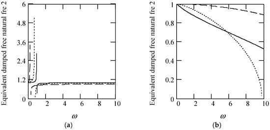
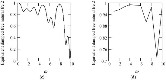
Figure 15.
Illustrations of ωeqd2 for m = 1, c = 1, and k = 1. (a). ωeqd2 for β(ω) = 0.3 (solid), 0.6 (dot), 0.9 (dash). (b). ωeqd2 when β(ω) = 1.3 (solid), 1.6 (dot), 1.9 (dash). (c). ωeqd2 when β(ω) = 1.2 + 0.5cos(2ω). (d). ωeqd2 when β(ω) is a uniformly distributed random function with the range (0.3, 1.7).
4.2.6. Equivalent Frequency Ratio of Type 2 Multi-Fractional Vibrator
Denote by γeq2 the equivalent frequency ratio of a type 2 multi-fractional vibrator. Define it by
Theorem 18 (Equivalent frequency ratio 2).
Let γ be the primary frequency ratio. The quantity γeq2 is expressed by
Proof.
When substituting ωeqn2 into (58), we have (59). This finishes the proof. □
We show some plots of γeq2 in Figure 16.
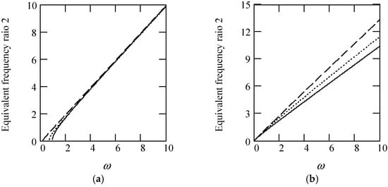
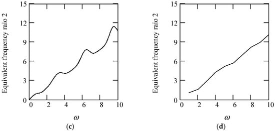
Figure 16.
Plots of γeq2 for m = 1, c = 1, and k = 1. (a). ωeqd2 for β(ω) = 0.3 (solid), 0.6 (dot), 0.9 (dash). (b). γeq2 when β(ω) = 1.3 (solid), 1.6 (dot), 1.9 (dash). (c). γeq2 when β(ω) = 1.2 + 0.5cos(2ω). (d). γeq2 when β(ω) is a uniformly distributed random function with the range (0.3, 1.7).
4.3. Frequency Transfer Function of Type 2 Multi-Fractional Vibrator
Based on the notations of meq2, ceq2, ζeq2, and ωeqn2, we write the motion phasor equation of type 2 multi-fractional vibrators in the form
Theorem 19 (Frequency transfer function 2).
Let H2(ω) be the frequency transfer function in phasor for a type 2 multi-fractional vibrator. Then,
Proof.
From (60), we have
Substituting meq2, ζeq2, and ωeqn2 into the right side of the above equation yields (61). The proof is finished. □
When using γeq2 and ζeq2, we can rewrite the above by
The amplitude of H2(ω) is in the form
which equals to
The phase of H2(ω) is given by
Thus,
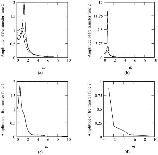
Figure 17.
Plots of |H2(ω)| for m = 1, c = 1, and k = 1. (a). |H2(ω)| for β(ω) = 0.3 (solid), 0.6 (dot), 0.9 (dash). (b). |H2(ω)| when β(ω) = 1.3 (solid), 1.6 (dot), 1.9 (dash). (c). |H2(ω)| when β(ω) = 1.2 + 0.5cos(2ω). (d). |H2(ω)| when β(ω) is a uniformly distributed random function with the range (0.3, 1.7).
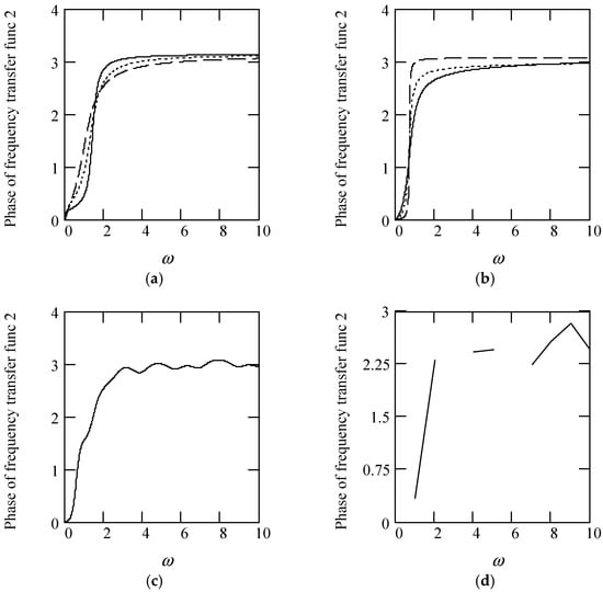
Figure 18.
Plots of φ2(ω) for m = 1, c = 1, and k = 1. (a). φ2(ω) for β(ω) = 0.3 (solid), 0.6 (dot), 0.9 (dash). (b). φ2(ω) when β(ω) = 1.3 (solid), 1.6 (dot), 1.9 (dash). (c). φ2(ω) when β(ω) = 1.2 + 0.5cos(2ω). (d). φ2(ω) when β(ω) is a uniformly distributed random function with the range (0.3, 1.7).
4.4. Stationary Response to Sinusoidal Vibration of Type 2 Multi-Fractional Vibrator
Regarding a type 2 multi-fractional vibrator, there are two expressions of stationary sinusoidal response. One is the response in the phasor domain, see Theorem 20, and the other in the time domain, see Theorem 21.
Theorem 20 (Response phasor 2).
The response phasor of a type 2 multi-fractional vibrator is given by
Proof.
Since X2 = H2(ω)F, according to Theorem 19, we have the above. The proof is finished. □
Equation (68) can be expressed by
Theorem 21 (Stationary sinusoidal response 2).
The stationary sinusoidal response to a type 2 multi-fractional vibrator is given by
Proof.
Because x2(t) = Im[X2exp(iωt)], X2 = H2(ω)F, and F = F0exp(iθ), we have x2(t) = Im[H2(ω)F0exp(iθ)exp(iωt)] = Im{|H2(ω)|F0exp(iωt)exp(iθ)exp[−iφ(ω)]}. Thus, the above holds. The proof is finished. □
Some plots of x2(t) are shown in Figure 19 and Figure 20, where we see that the effect of fractional order β(ω) on the sinusoidal response x2(t) is considerable.
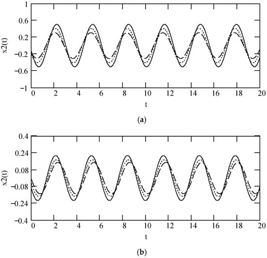
Figure 19.
Plots of x2(t) when ω = 2, F0 = 1, θ = 0, m = 1, c = 1, and k = 1. (a). x2(t) for β = 0.3 (solid), 0.6 (dot), and 0.9 (dash). (b). x2(t) for β = 1.3 (solid), 1.6 (dot), and 1.9 (dash).
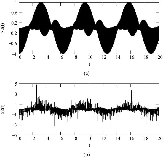
Figure 20.
Plots of x2(t) when F0 = 1, θ = 0, m = 1, c = 1, and k = 1. (a). x2(t) for β(ω) = 1.2 + 0.5cos(2ω). (b). x2(t) when β(ω) is a uniformly distributed random function with the range (0.3, 1.7).
5. Results in Type 3 Multi-Fractional Vibrators
We present the results with respect to type 3 multi-fractional vibrators in four folds. We show the motion phasor equation of a type 3 multi-fractional vibrator in Section 5.1. The expressions of equivalent vibration parameters about a type 3 multi-fractional vibrator are discussed in Section 5.2. The expression of frequency transfer function of a type 3 multi-fractional vibrator is explained in Section 5.3. The expressions of stationary sinusoidal response to a type 3 multi-fractional vibrator in the phasor domain and the time one are put forward in Section 5.4.
5.1. Motion Phasor Equation of Type 3 Multi-Fractional Vibrator
A system that follows
is called a type 3 multi-fractional vibrator. The theorem below gives its motion phasor equation.
Theorem 22 (Motion phasor equation 3).
Denote by X3 the phasor of response x3(t) of a type 3 multi-fractional vibrator. Let F be the phasor of excitation f(t) = F0sin(ωt + θ). Then, the motion phasor equation of a type 3 multi-fractional vibrator is expressed by
Proof.
Using phasor to express both sides of (71) yields (72). This completes the proof. □
Considering the principal branches of iα and iβ, we express the left side of (72) by
The right side of the above can be written by
Therefore,
5.2. Equivalent Parameters of Type 3 Multi-Fractional Vibrator
In this Subsection, we present the expressions of equivalent vibration parameters of a type 3 multi-fractional vibrator. Those parameters are equivalent mass, equivalent damping, equivalent damping ratio, equivalent damping free natural angular frequency, equivalent damped natural angular frequency, and equivalent frequency ratio.
5.2.1. Equivalent Mass of Type 3 Multi-Fractional Vibrator
Theorem 23 (Equivalent mass 3).
Let meq3 be the equivalent mass of a multi-fractional vibrator of type 3. Then,
Proof.
The first item on the right side of (75) stands for equivalent mass. This finishes the proof. □
Figure 21 illustrates some plots of meq3.
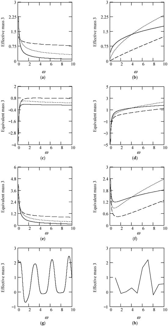
Figure 21.
Plots of meq3 for m = 1 and c = 1. (a). meq3 with β(ω) = 1 for α(ω) = 1.3 (solid), 1.6 (dot), 1.9 (dash). (b). meq3 with β(ω) = 1 for α(ω) = 2.3 (solid), 2.6 (dot), 2.9 (dash). (c). meq3 with β(ω) = 0.8 for α(ω) = 1.3 (solid), 1.6 (dot), 1.9 (dash). (d). meq3 with β(ω) = 0.8 for α(ω) = 2.3 (solid), 2.6 (dot), 2.9 (dash). (e). meq3 with β(ω) = 1.2 for α(ω) = 1.3 (solid), 1.6 (dot), 1.9 (dash). (f). meq3 with β(ω) = 1.2 for α(ω) = 2.3 (solid), 2.6 (dot), 2.9 (dash). (g). meq3 when α(ω) = 1.4 + cos(2ω) and β(ω) = 1.2 + 0.5cos(2ω). (h). meq3 when α(ω) is a uniformly distributed random function with the range (0.3, 2.7) and β(ω) is a uniformly distributed random function with the range (0.3, 1.7).
5.2.2. Equivalent Damping of Type 3 Multi-Fractional Vibrator
Theorem 24 (Equivalent damping 3).
Let ceq3 be the equivalent damping of a multi-fractional vibrator of type 3. Then,
Proof.
From the second item on the right side of (75), we see that the above is true. The proof is finished. □
Some plots of ceq3 are indicated in Figure 22.
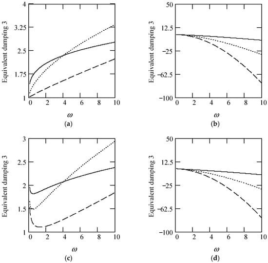
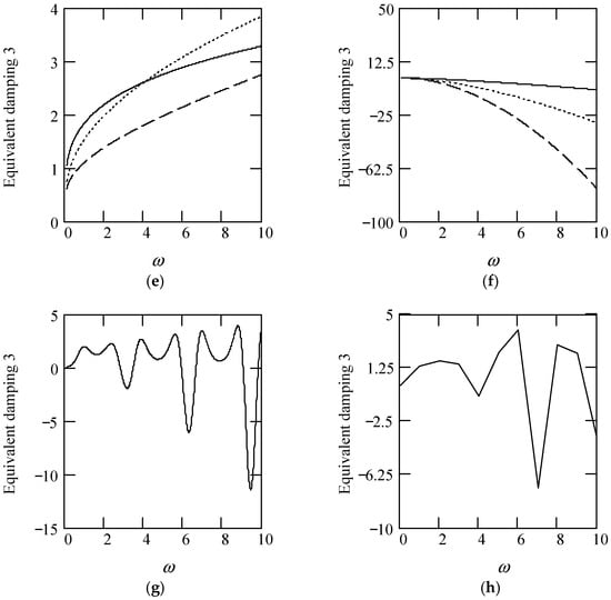
Figure 22.
Plots of ceq3 for m = 1 and c = 1. (a). ceq3 with β(ω) = 1 for α(ω) = 1.3 (solid), 1.6 (dot), 1.9 (dash). (b). ceq3 with β(ω) = 1 for α(ω) = 2.3 (solid), 2.6 (dot), 2.9 (dash). (c). ceq3 with β(ω) = 0.8 for α(ω) = 1.3 (solid), 1.6 (dot), 1.9 (dash). (d). ceq3 with β(ω) = 0.8 for α(ω) = 2.3 (solid), 2.6 (dot), 2.9 (dash). (e). ceq3 with β(ω) = 1.2 for α(ω) = 1.3 (solid), 1.6 (dot), 1.9 (dash). (f). ceq3 with β(ω) = 1.2 for α(ω) = 2.3 (solid), 2.6 (dot), 2.9 (dash). (g). ceq3 when α(ω) = 1.4 + cos(2ω) and β(ω) = 1.2 + 0.5cos(2ω). (h). ceq3 when α(ω) is a uniformly distributed random function with the range (0.3, 2.7) and β(ω) is a uniformly distributed random function with the range (0.3, 1.7).
5.2.3. Equivalent Damping Ratio of Type 3 Multi-Fractional Vibrator
Theorem 25 (Equivalent damping ratio 3).
Let ζeq3 be the equivalent damping ratio of a type 3 multi-fractional vibrator. Define it by
Then,
Proof.
Substituting meq3 and ceq3 into (78) results in (79). The proof is finished. □
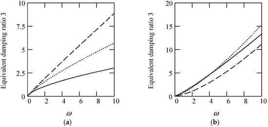
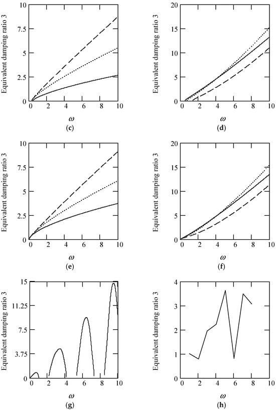
Some plots of ζeq3 are shown in Figure 23.
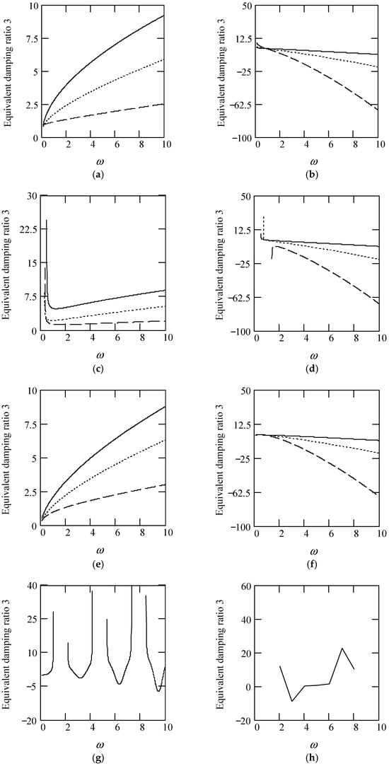
Figure 23.
Plots of ζeq3 for m = 1, c = 1, and k = 1. (a). ζeq3 with β(ω) = 1 for α(ω) = 1.3 (solid), 1.6 (dot), 1.9 (dash). (b). ζeq3 with β(ω) = 1 for α(ω) = 2.3 (solid), 2.6 (dot), 2.9 (dash). (c). ζeq3 with β(ω) = 0.8 for α(ω) = 1.3 (solid), 1.6 (dot), 1.9 (dash). (d). ζeq3 with β(ω) = 0.8 for α(ω) = 2.3 (solid), 2.6 (dot), 2.9 (dash). (e). ζeq3 with β(ω) = 1.2 for α(ω) = 1.3 (solid), 1.6 (dot), 1.9 (dash). (f). ζeq3 with β(ω) = 1.2 for α(ω) = 2.3 (solid), 2.6 (dot), 2.9 (dash). (g). ζeq3 when α(ω) = 1.4 + cos(2ω) and β(ω) = 1.2 + 0.5cos(2ω). (h). ζeq3 when α(ω) is a uniformly distributed random function with the range (0.3, 2.7) and β(ω) is a uniformly distributed random function with the range (0.3, 1.7).
5.2.4. Equivalent Damping Free Natural Angular Frequency of Type 3 Multi-Fractional Vibrator
Theorem 26 (Equivalent damping free natural angular frequency 3).
Denote by ωeqn3 the equivalent damping free natural angular frequency of a type 3 multi-fractional vibrator. Define it by
Then
Proof.
Substituting meq3 into (80) yields (81). The proof is finished. □
Some plots of ωeqn3 are illustrated in Figure 24.
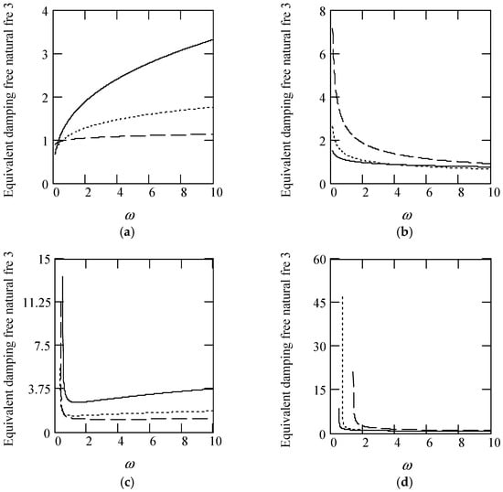
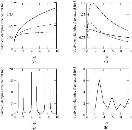
Figure 24.
Plots of ωeqn3 for m = 1, c = 1, and k = 1. (a). ωeqn3 with β(ω) = 1 for α(ω) = 1.3 (solid), 1.6 (dot), 1.9 (dash). (b). ωeqn3 with β(ω) = 1 for α(ω) = 2.3 (solid), 2.6 (dot), 2.9 (dash). (c). ωeqn3 with β(ω) = 0.8 for α(ω) = 1.3 (solid), 1.6 (dot), 1.9 (dash). (d). ωeqn3 with β(ω) = 0.8 for α(ω) = 2.3 (solid), 2.6 (dot), 2.9 (dash). (e). ωeqn3 with β(ω) = 1.2 for α(ω) = 1.3 (solid), 1.6 (dot), 1.9 (dash). (f). ωeqn3 with β(ω) = 1.2 for α(ω) = 2.3 (solid), 2.6 (dot), 2.9 (dash). (g). ωeqn3 when α(ω) = 1.4 + cos(2ω) and β(ω) = 1.2 + 0.5cos(2ω). (h). ωeqn3 when α(ω) is a uniformly distributed random function with the range (0.3, 2.7) and β(ω) is a uniformly distributed random function with the range (0.3, 1.7).
5.2.5. Equivalent Damped Natural Angular Frequency of Type 3 Multi-Fractional Vibrator
From a practical view of vibration engineering, one is interested in small damping. Therefore, we adopt |ζeq3| ≤ 1 in what follows.
Theorem 27 (Equivalent damped natural angular frequency 3).
Denote by ωeqd3 the equivalent damped natural angular frequency of a multi-fractional vibrator of type 3. Then,
Thus,
Proof.
Substituting ζeq3 and ωeqn3 into (82) produces (83). This finishes the proof. □
Figure 25 indicates some plots of ωeqd3.
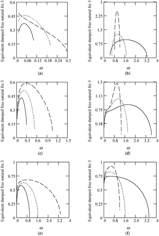
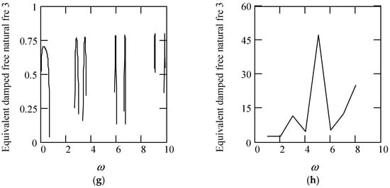
Figure 25.
Plots of ωeqd3 for m = 1, c = 1, and k = 1. (a). ωeqd3 with β(ω) = 1 for α(ω) = 1.3 (solid), 1.6 (dot), 1.9 (dash). (b). ωeqd3 with β(ω) = 1 for α(ω) = 2.3 (solid), 2.6 (dot), 2.9 (dash). (c). ωeqd3 with β(ω) = 1.2 for α(ω) = 1.3 (solid), 1.6 (dot), 1.9 (dash). (d). ωeqd3 with β(ω) = 1.8 for α(ω) = 2.3 (solid), 2.6 (dot), 2.9 (dash). (e). ωeqd3 with β(ω) = 1.2 for α(ω) = 1.3 (solid), 1.6 (dot), 1.9 (dash). (f). ωeqd3 with β(ω) = 1.2 for α(ω) = 2.3 (solid), 2.6 (dot), 2.9 (dash). (g). ωeqd3 when α(ω) = 1.4 + cos(2ω) and β(ω) = 1.2 + 0.5cos(2ω). (h). ωeqd3 when α(ω) is a uniformly distributed random function with the range (0.3, 2.7) and β(ω) is a uniformly distributed random function with the range (0.3, 1.7).
5.2.6. Equivalent Frequency Ratio of Type 3 Multi-Fractional Vibrator
Theorem 28 (Equivalent frequency ratio 3).
Let γeq3 be the equivalent frequency ratio of a multi-fractional vibrator of type 3. Define it by
Then,
Proof.
Substituting ωeqn3 into (84) results in (85). The proof is finished. □
Some plots of γeq3 are shown in Figure 26.
Figure 26.
Plots of γeq3 for m = 1, c = 1, and k = 1. (a). γeq3 with β(ω) = 1 for α(ω) = 1.3 (solid), 1.6 (dot), 1.9 (dash). (b). γeq3 with β(ω) = 1 for α(ω) = 2.3 (solid), 2.6 (dot), 2.9 (dash). (c). γeq3 with β(ω) = 0.8 for α(ω) = 1.3 (solid), 1.6 (dot), 1.9 (dash). (d). γeq3 with β(ω) = 0.8 for α(ω) = 2.3 (solid), 2.6 (dot), 2.9 (dash). (e). γeq3 with β(ω) = 1.2 for α(ω) = 1.3 (solid), 1.6 (dot), 1.9 (dash). (f). γeq3 with β(ω) = 1.2 for α(ω) = 2.3 (solid), 2.6 (dot), 2.9 (dash). (g). γeq3 when α(ω) = 1.4 + cos(2ω) and β(ω) = 1.2 + 0.5cos(2ω). (h). γeq3 when α(ω) is a uniformly distributed random function with the range (0.3, 2.7) and β(ω) is a uniformly distributed random function with the range (0.3, 1.7).
5.3. Frequency Transfer Function of Type 3 Multi-Fractional Vibrator
Theorem 29 (Frequency transfer function 3).
Let H3(ω) be the frequency transfer function in phasor for a type 3 multi-fractional vibrator. Then,
Proof.
The motion phasor equation can be written by
Thus,
Substituting meq3 and ceq3 into the right side of the above yields (86). The proof is finished. □
Using γeq3 and ζeq3, H3(ω) can be written by
The amplitude of H3(ω) is in the form
which is equivalent to
The phase of H3(ω) is given by
Thus,
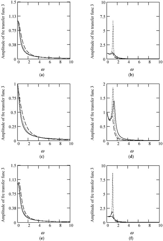
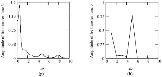
Figure 27.
Plots of |H3(ω)| for m = 1, c = 1, and k = 1. (a). γeq3 with β(ω) = 1 for α(ω) = 1.3 (solid), 1.6 (dot), 1.9 (dash). (b). |H3(ω)| with β(ω) = 1 for α(ω) = 2.3 (solid), 2.6 (dot), 2.9 (dash). (c). |H3(ω)| with β(ω) = 0.8 for α(ω) = 1.3 (solid), 1.6 (dot), 1.9 (dash). (d). |H3(ω)| with β(ω) = 0.8 for α(ω) = 2.3 (solid), 2.6 (dot), 2.9 (dash). (e). |H3(ω)| with β(ω) = 1.2 for α(ω) = 1.3 (solid), 1.6 (dot), 1.9 (dash). (f). |H3(ω)| with β(ω) = 1.2 for α(ω) = 2.3 (solid), 2.6 (dot), 2.9 (dash). (g). |H3(ω)| when α(ω) = 1.4 + cos(2ω) and β(ω) = 1.2 + 0.5cos(2ω). (h). |H3(ω)| when α(ω) is a uniformly distributed random function with the range (0.3, 2.7) and β(ω) is a uniformly distributed random function with the range (0.3, 1.7).
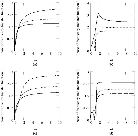
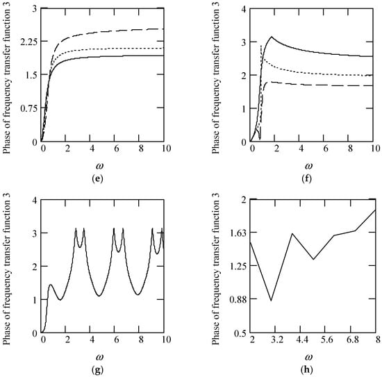
Figure 28.
Plots of φ3(ω) for m = 1, c = 1, and k = 1. (a). γeq3 with β(ω) = 1 for α(ω) = 1.3 (solid), 1.6 (dot), 1.9 (dash). (b). φ3(ω) with β(ω) = 1 for α(ω) = 2.3 (solid), 2.6 (dot), 2.9 (dash). (c). φ3(ω) with β(ω) = 0.5 for α(ω) = 1.3 (solid), 1.6 (dot), 1.9 (dash). (d). φ3(ω) with β(ω) = 0.5 for α(ω) = 2.3 (solid), 2.6 (dot), 2.9 (dash). (e). φ3(ω) with β(ω) = 1.5 for α(ω) = 1.3 (solid), 1.6 (dot), 1.9 (dash). (f). φ3(ω) with β(ω) = 1.5 for α(ω) = 2.3 (solid), 2.6 (dot), 2.9 (dash). (g). φ3(ω) when α(ω) = 1.4 + cos(2ω) and β(ω) = 1.2 + 0.5cos(2ω). (h). φ3(ω) when α(ω) is a uniformly distributed random function with the range (0.3, 2.7) and β(ω) is a uniformly distributed random function with the range (0.3, 1.7).
5.4. Stationary Response to Sinusoidal Vibration of Type 3 Multi-Fractional Vibrator
We bring forward two expressions of stationary sinusoidal response to a type 3 multi-fractional vibrator. One is the response in phasor and the other the response in time. They are expressed by Theorems 30 and 31, respectively.
Theorem 30 (Response phasor 3).
The response phasor of a type 3 multi-fractional vibrator is expressed by
Proof.
As X3 = H3(ω)F, we have the above. The proof is finished. □
Equation (94) can be in the form
Theorem 31 (Stationary sinusoidal response 3).
The stationary sinusoidal response of a type 3 multi-fractional vibrator is expressed by
Proof.
Since x3(t) = Im[X3exp(iωt)], X3 = H3(ω)F, and F = F0exp(iθ), we have x3(t) = Im{|H3(ω)|F0exp(iωt)exp(iθ)exp[−iφ(ω)]}. Therefore, the above is valid. The proof is finished. □
Figure 29 indicates some plots of x3(t). It shows that there is a significant effect of fractional orders α(ω) and β(ω) on the sinusoidal response x3(t).
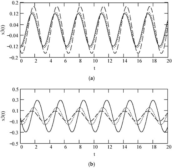
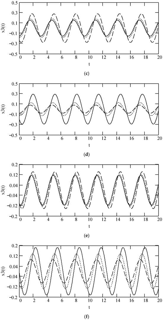
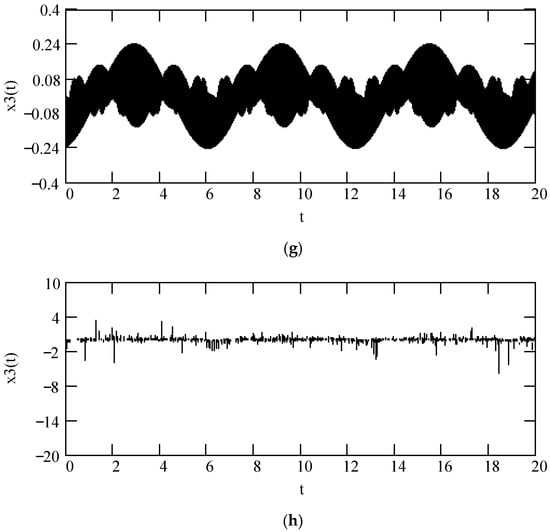
Figure 29.
Plots of x3(t) when ω = 2, F0 = 1, θ = 0, m = 1, and k = 1. (a). β = 1, α = 1.3 (solid), 1.6 (dot), and 1.9 (dash). (b). β = 1, α = 2.3 (solid), 2.6 (dot), and 2.9 (dash). (c). β = 0.5, α = 1.3 (solid), 1.6 (dot), and 1.9 (dash). (d). β = 0.5, α = 2.3 (solid), 2.6 (dot), and 2.9 (dash). (e). β = 1.5, α = 1.3 (solid), 1.6 (dot), and 1.9 (dash). (f). β = 1.5, α = 2.3 (solid), 2.6 (dot), and 2.9 (dash). (g). x3(t) when α(ω) = 1.4 + cos(2ω) and β(ω) = 1.2 + 0.5cos(2ω). (h). x3(t) when α(ω) is a uniformly distributed random function with the range (0.3, 2.7) and β(ω) is a uniformly distributed random function with the range (0.3, 1.7).
6. Results about Type 4 Multi-Fractional Vibrators
Now, we propose the results regarding type 4 multi-fractional vibrators in four aspects. The motion phasor equation of a type 4 multi-fractional vibrator is proposed in Section 6.1. The expressions of equivalent vibration parameters about a type 4 multi-fractional vibrator are given in Section 6.2. The expression of frequency transfer function of a type 4 multi-fractional vibrator is in Section 6.3. The expressions of stationary sinusoidal response to a type 4 multi-fractional vibrator in the phasor domain and the time one are brought forward in Section 6.4.
6.1. Motion Phasor Equation of Type 4 Multi-Fractional Vibrator
Theorem 32 (Motion phasor equation 4).
Let X4 be the phasor of response x4(t) of a type 4 multi-fractional vibrator. Denote by F the phasor of excitation f(t) = F0sin(ωt + θ). Then, the motion phasor equation of a type 4 multi-fractional vibrator is in the form
Proof.
Using phasor to express both sides of yields (97). The proof is finished. □
Taking into account the principal branches of iα and iλ, we write the left side of the above equation by
The right side of the above can be written by
Therefore,
Note that stands for a fractional restoration force. Hence, 0 ≤ λ(ω) < 1.
6.2. Equivalent Parameters of Type 4 Multi-Fractional Vibrator
The present results below are the expressions of equivalent vibration parameters of a type 4 multi-fractional vibrator. They are equivalent mass in Section 6.2.1, equivalent damping in Section 6.2.2, equivalent stiffness in Section 6.2.3, equivalent damping ratio in Section 6.2.4, equivalent damping free natural angular frequency in Section 6.2.5, equivalent damped natural angular frequency in Section 6.2.6, and equivalent frequency ratio in Section 6.2.7.
6.2.1. Equivalent Mass of Type 4 Multi-Fractional Vibrator
Theorem 33 (Equivalent mass 4).
Denote by meq4 the equivalent mass for a type 4 multi-fractional vibrator. Then,
Proof.
From the first item on the right side of (100), we see that the above is true. The proof is finished. □
6.2.2. Equivalent Damping of Type 4 Multi-Fractional Vibrator
Theorem 34 (Equivalent damping 4).
Let ceq4 be the equivalent damping of a multi-fractional vibrator of type 4. Then,
Proof.
The second item on the right side of (100) implies that the above holds. The proof is finished. □
Refer Figure 30 for some plots of ceq4.
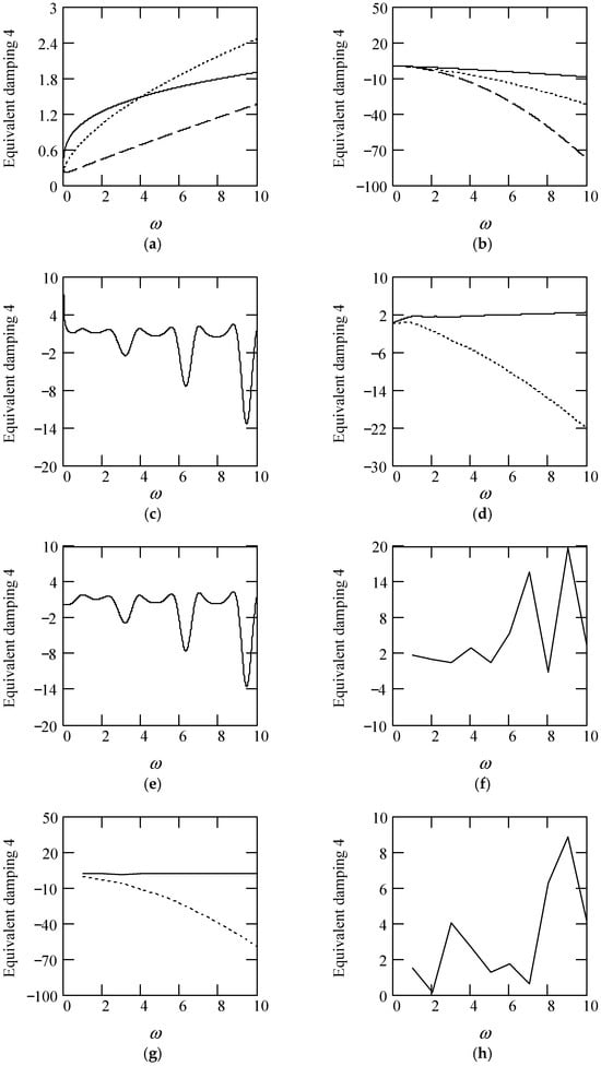
Figure 30.
Plots of ceq4 when m = 1, k = 1. (a). ceq4 for λ(ω) = 0.9 when α(ω) = 1.3 (solid), 1.6 (dot), 1.9 (dash). (b). ceq4 for λ(ω) = 0.9 when α(ω) = 2.3 (solid), 2.6 (dot), 2.9 (dash). (c). ceq4 for α(ω) = 1.4 + cos(2ω) and λ(ω) = 0.5. (d). ceq4 for λ(ω) = 0.5 + 0.4cos(2ω) and α(ω) = 1.5 (solid), 2.5 (dot). (e). ceq4 for α(ω) = 1.4 + cos(2ω) and λ(ω) = 0.5 + 0.4cos(2ω). (f). ceq4 for λ(ω) = 0.5 and α(ω) is a uniformly distributed random function with the range (0.3, 2.7). (g). ceq4 for α(ω) = 1.2 (solid), 2.8 (dot), when λ(ω) is a uniformly distributed random function with the range (0.1, 0.9). (h). ceq4 when α(ω) is a uniformly distributed random function with the range (0.3, 2.7) and λ(ω) is a uniformly distributed random function with the range (0.1, 0.9).
6.2.3. Equivalent Stiffness of Type 4 Multi-Fractional Vibrator
Theorem 35 (Equivalent stiffness 4).
Denote by keq4 the equivalent stiffness of a type 4multi-fractional vibrator. Then,
Proof.
From the third item on the right side of (100), we see that the above is valid. The proof is finished. □
Refer to Figure 31 for some plots of keq4.
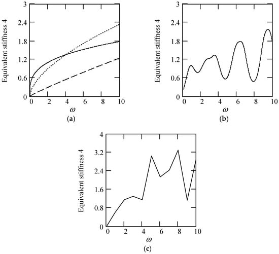
Figure 31.
Plots of keq4 for k = 1. (a). keq4 when λ(ω) = 0.3 (solid), 0.6 (dot), 0.9 (dash). (b). keq4 when λ(ω) = 1.4 + cos(2ω). (c). keq4 when λ(ω) is a uniformly distributed random function with the range (0.1, 0.9).
6.2.4. Equivalent Damping Ratio of Type 4 Multi-Fractional Vibrator
Theorem 36 (Equivalent damping ratio 4).
Denote by ζeq4 the equivalent damping ratio of a type 4 multi-fractional vibrator. Define it by
Then,
Proof.
Substituting meq4, ceq4, and keq4 into (104) yields (105). This finishes the proof. □
Some plots of ζeq4 are shown in Figure 32.
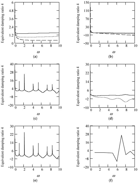
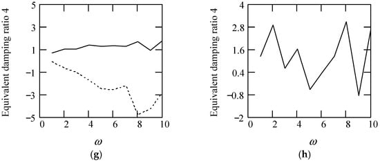
Figure 32.
Plots of ζeq4 when m = 1, k = 1. (a). ζeq4 for λ(ω) = 0.9 when α(ω) = 1.3 (solid), 1.6 (dot), 1.9 (dash). (b). ζeq4 for λ(ω) = 0.9 when α(ω) = 2.3 (solid), 2.6 (dot), 2.9 (dash). (c). ζeq4 for α(ω) = 1.4 + cos(2ω) and λ(ω) = 0.5. (d). ζeq4 for λ(ω) = 0.5 + 0.4cos(2ω) and α(ω) = 1.5 (solid), 2.5 (dot). (e). ζeq4 for α(ω) = 1.4 + cos(2ω) and λ(ω) = 0.5 + 0.4cos(2ω). (f). ζeq4 for λ(ω) = 0.5 and α(ω) is a uniformly distributed random function with the range (0.3, 2.7). (g). ζeq4 for α(ω) = 1.5 (solid), 2.5 (dot), when λ(ω) is a uniformly distributed random function with the range (0.1, 0.9). (h). ζeq4 when α(ω) is a uniformly distributed random function with the range (0.3, 2.7) and λ(ω) is a uniformly distributed random function with the range (0.1, 0.9).
6.2.5. Equivalent Damping Free Natural Angular Frequency of Type 4 Multi-Fractional Vibrator
Theorem 37 (Equivalent damping free natural angular frequency 4).
Let ωeqn4 be the equivalent damping free natural angular frequency of a type 4 multi-fractional vibrator. Define it by
Then,
Proof.
Substituting meq4 and keq4 into (106) produces (107). This finishes the proof. □
Figure 33 illustrates some plots of ωeqn4.
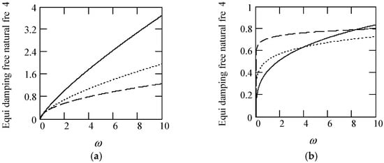
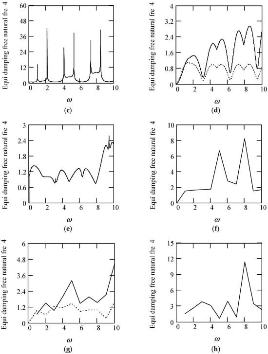
Figure 33.
Plots of ωeqn4 when m = 1, k = 1. (a). ωeqn4 for λ(ω) = 0.9 when α(ω) = 1.3 (solid), 1.6 (dot), 1.9 (dash). (b). ωeqn4 for λ(ω) = 0.9 when α(ω) = 2.3 (solid), 2.6 (dot), 2.8 (dash). (c). ωeqn4 for α(ω) = 1.4 + cos(2ω) and λ(ω) = 0.5. (d). ωeqn4 for λ(ω) = 0.5 + 0.4cos(2ω) and α(ω) = 1.5 (solid), 2.5 (dot). (e). ωeqn4 for α(ω) = 1.4 + cos(2ω) and λ(ω) = 0.5 + 0.4cos(2ω). (f). ωeqn4 for λ(ω) = 0.5 and α(ω) is a uniformly distributed random function with the range (0.3, 2.7). (g). ωeqn4 for α(ω) = 1.5 (solid), 2.5 (dot), when λ(ω) is a uniformly distributed random function with the range (0.1, 0.9). (h). ωeqn4 when α(ω) is a uniformly distributed random function with the range (0.3, 2.7) and λ(ω) is a uniformly distributed random function with the range (0.1, 0.9).
6.2.6. Equivalent Damped Natural Angular Frequency of Type 4 Multi-Fractional Vibrator
From the point of view of practical vibrations, we adopt |ζeq4| ≤ 1 in what follows.
Theorem 38 (Equivalent damped natural angular frequency 4).
Let ωeqd4 be the equivalent damped natural angular frequency of a multi-fractional vibrator of type 4. Define it by
Then,
Proof.
Substituting ζeq4 and ωeqn4 into (108) results in (109). The proof is finished. □
Figure 34 shows some plots of ωeqd4.
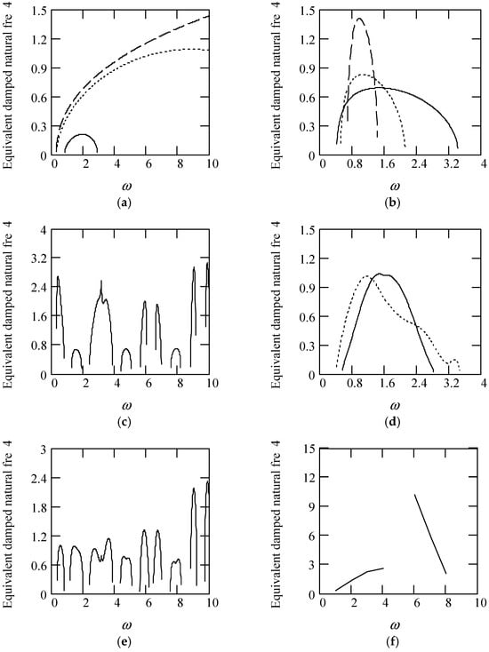
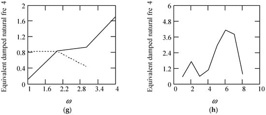
Figure 34.
Plots of ωeqd4 when m = 1, k = 1. (a). ωeqd4 for λ(ω) = 0.8 when α(ω) = 1.5 (solid), 1.7 (dot), 1.9 (dash). (b). ωeqd4 for λ(ω) = 0.8 when α(ω) = 2.5 (solid), 2.7 (dot), 2.9 (dash). (c). ωeqd4 for α(ω) = 1.4 + cos(2ω) and λ(ω) = 0.5. (d). ωeqd4 for λ(ω) = 0.5 + 0.4cos(2ω) and α(ω) = 1.5 (solid), 2.5 (dot). (e). ωeqd4 for α(ω) = 1.4 + cos(2ω) and λ(ω) = 0.5 + 0.4cos(2ω). (f). ωeqd4 for λ(ω) = 0.5 and α(ω) is a uniformly distributed random function with the range (0.3, 2.7). (g). ωeqd4 for α(ω) = 1.5 (solid), 2.5 (dot), when λ(ω) is a uniformly distributed random function with the range (0.1, 0.9). (h). ωeqd4 when α(ω) is a uniformly distributed random function with the range (0.3, 2.7) and λ(ω) is a uniformly distributed random function with the range (0.1, 0.9).
6.2.7. Equivalent Frequency Ratio of Type 4 Multi-Fractional Vibrator
Theorem 39 (Frequency ratio 4).
Denote by γeq4 the equivalent frequency ratio of a multi-fractional vibrator of type 4. It is defined by
Then,
Proof.
Substituting ωeqn4 into (110) produces (111). This finishes the proof. □
Some plots of γeq4 are illustrated in Figure 35.
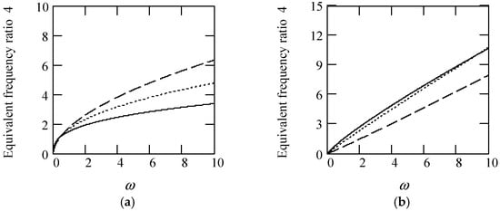
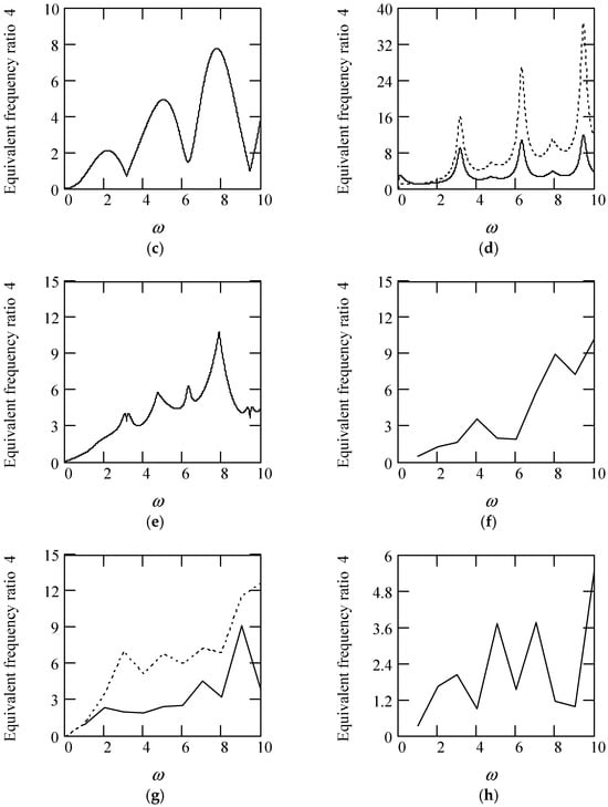
Figure 35.
Plots of γeq4 when m = 1, k = 1. (a). γeq4 for λ(ω) = 0.8 when α(ω) = 1.5 (solid), 1.7 (dot), 1.9 (dash). (b). γeq4 for λ(ω) = 0.8 when α(ω) = 2.5 (solid), 2.7 (dot), 2.9 (dash). (c). γeq4 for α(ω) = 1.4 + cos(2ω) and λ(ω) = 0.5. (d). γeq4 for λ(ω) = 0.5 + 0.4cos(2ω) and α(ω) = 1.5 (solid), 2.5 (dot). (e). γeq4 for α(ω) = 1.4 + cos(2ω) and λ(ω) = 0.5 + 0.4cos(2ω). (f). γeq4 for λ(ω) = 0.5 and α(ω) is a uniformly distributed random function with the range (0.3, 2.7). (g). γeq4 for α(ω) = 1.5 (solid), 2.5 (dot), when λ(ω) is a uniformly distributed random function with the range (0.1, 0.9). (h). γeq4 when α(ω) is a uniformly distributed random function with the range (0.3, 2.7) and λ(ω) is a uniformly distributed random function with the range (0.1, 0.9).
6.3. Frequency Transfer Function of Type 4 Multi-Fractional Vibrator
Theorem 40 (Frequency transfer function 4).
Denote by H4(ω) the frequency transfer function in phasor for a type 4 multi-fractional vibrator. Then,
Proof.
When writing the motion phasor equation by
we have
Substituting meq4, ceq4 and keq4 into the above produces (112). The proof is finished. □
With γeq4 and ζeq4, we can write the above by
The amplitude of H4(ω) is
The phase of H4(ω) is
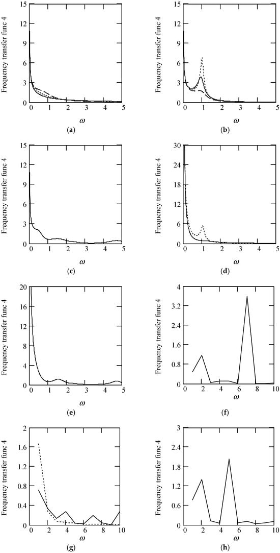
Figure 36.
Plots of |H4(ω)| when m = 1, k = 1. (a). |H4(ω)| for λ(ω) = 0.5 when α(ω) = 1.3 (solid), 1.6 (dot), 1.9 (dash). (b). |H4(ω)| for λ(ω) = 0.5 when α(ω) = 2.3 (solid), 2.6 (dot), 2.9 (dash). (c). |H4(ω)| for α(ω) = 1.4 + cos(2ω) and λ(ω) = 0.5. (d). |H4(ω)| for λ(ω) = 0.5 + 0.4cos(2ω) and α(ω) = 1.5 (solid), 2.5 (dot). (e). |H4(ω)| for α(ω) = 1.4 + cos(2ω) and λ(ω) = 0.5 + 0.4cos(2ω). (f). |H4(ω)| for λ(ω) = 0.5 and α(ω) is a uniformly distributed random function with the range (0.3, 2.7). (g). |H4(ω)| for α(ω) = 1.5 (solid), 2.5 (dot), when λ(ω) is a uniformly distributed random function with the range (0.1, 0.9). (h). |H4(ω)| when α(ω) is a uniformly distributed random function with the range (0.3, 2.7) and λ(ω) is a uniformly distributed random function with the range (0.1, 0.9).
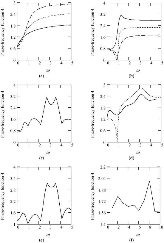
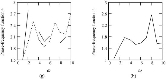
Figure 37.
Plots of φ4(ω). (a). φ4(ω) for λ(ω) = 0.5 when α(ω) = 1.3 (solid), 1.6 (dot), 1.9 (dash). (b). φ4(ω) for λ(ω) = 0.5 when α(ω) = 2.3 (solid), 2.6 (dot), 2.9 (dash). (c). φ4(ω) for α(ω) = 1.4 + cos(2ω) and λ(ω) = 0.5. (d). φ4(ω) for λ(ω) = 0.5 + 0.4cos(2ω) and α(ω) = 1.5 (solid), 2.5 (dot). (e). φ4(ω) for α(ω) = 1.4 + cos(2ω) and λ(ω) = 0.5 + 0.4cos(2ω). (f). φ4(ω) for λ(ω) = 0.5 and α(ω) is a uniformly distributed random function with the range (0.3, 2.7). (g). φ4(ω) for α(ω) = 1.5 (solid), 2.5 (dot), when λ(ω) is a uniformly distributed random function with the range (0.1, 0.9). (h). φ4(ω) when α(ω) is a uniformly distributed random function with the range (0.3, 2.7) and λ(ω) is a uniformly distributed random function with the range (0.1, 0.9).
6.4. Stationary Response to Sinusoidal Vibration of Type 4 Multi-Fractional Vibrator
We propose two expressions of the stationary sinusoidal response to a type 4 multi-fractional vibrator. One is in the phasor domain and the other in the time domain. They are described by Theorems 41 and 42, respectively.
Theorem 41 (Response phasor 4).
The response phasor of a type 4 multi-fractional vibrator is expressed by
Proof.
Since X4 = H4(ω)F, we see that the above is true. The proof is finished. □
The above equation can be written by
Theorem 42 (Stationary sinusoidal response 4).
The stationary sinusoidal response to a type 4 multi-fractional vibrator is given by
Proof.
Since x4(t) = Im[X4exp(iωt)], X4 = H4(ω)F, F = F0exp(iθ), and
we have x4(t) = Im{|H4(ω)|F0exp(iωt)exp(iθ)exp[−iφ(ω)]}, which equals to (120). The proof is finished. □
In Figure 38, we show some plots of x4(t) for different values of α and λ. Figure 38 exhibits that there is significant effect of fractional orders α(ω) and λ(ω) on the sinusoidal response x4(t).
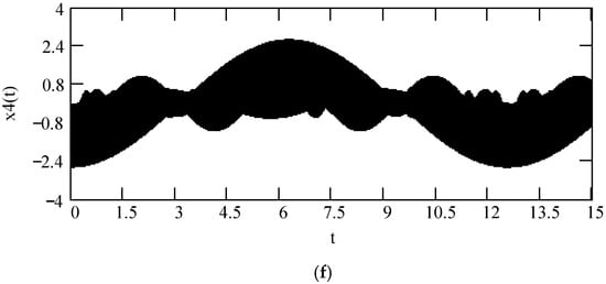
Figure 38.
Plots of x4(t) for F0 = 1, θ = 0, m = 1, and k = 1. (a). x4(t) when ω = 2 and λ(ω) = 0.5 when α(ω) = 1.3 (solid), 1.6 (dot), 1.9 (dash). (b). x4(t) when ω = 2 and λ(ω) = 0.5 when α(ω) = 2.3 (solid), 2.6 (dot), 2.9 (dash). (c). x4(t) for α(ω) = 1.4 + cos(2ω) and λ(ω) = 0.5. (d). x4(t) for λ(ω) = 0.5 + 0.4cos(2ω) and α(ω) = 1.5. (e). x4(t) for λ(ω) = 0.5 + 0.4cos(2ω) and α(ω) = 2.5. (f). x4(t) for α(ω) = 1.4 + cos(2ω) and λ(ω) = 0.5 + 0.4cos(2ω).
7. Results for Type 5 Multi-Fractional Vibrators
We now put forward the results with respect to type 5 multi-fractional vibrators. The motion phasor equation of a type 5 multi-fractional vibrator is presented in Section 7.1. The expressions of equivalent vibration parameters about a type 5 multi-fractional vibrator are discussed in Section 7.2. The expression of frequency transfer function of a type 5 multi-fractional vibrator is given in Section 7.3. The expressions of stationary sinusoidal response to a type 5 multi-fractional vibrator in the phasor domain and the time one are brought forward in Section 7.4.
7.1. Motion Phasor Equation of Type 5 Multi-Fractional Vibrator
Theorem 43 (Motion phasor equation 5).
Denote by X5 the phasor of response x5(t) of a type 5 multi-fractional vibrator. Let F be the phasor of excitation f(t) = F0sin(ωt + θ). The motion phasor equation of a type 5 multi-fractional vibrator is expressed by
Proof.
Using phasor to express both sides of produces the above. The proof is finished. □
Considering the principal branch of iλ, we express the left side of the above equation by
Rewriting the right side of the above by
we have
7.2. Equivalent Parameters of Type 5 Multi-Fractional Vibrator
We now present the expressions of equivalent vibration parameters of a type 5 multi-fractional vibrator, containing equivalent mass (Section 7.2.1), equivalent damping (Section 7.2.2), equivalent stiffness (Section 7.2.3), equivalent damping ratio (Section 7.2.4), equivalent damping free natural angular frequency (Section 7.2.5), equivalent damped natural angular frequency (Section 7.2.6), and equivalent frequency ratio (Section 7.2.7).
7.2.1. Equivalent Mass of Type 5 Multi-Fractional Vibrator
Theorem 44 (Equivalent mass 5).
Let meq5 be the equivalent mass of a type 5 multi-fractional vibrator. Then,
meq5 = m.
Proof.
From the first item on the right side of (124), we see that the above is true. This finishes the proof. □
7.2.2. Equivalent Damping of Type 5 Multi-Fractional Vibrator
Theorem 45 (Equivalent damping 5).
Denote by ceq5 the equivalent damping of a type 5 multi-fractional vibrator. Then,
Proof.
The second item on the right side of (124) exhibits that the above is true. The proof is finished. □
Some plots of ceq5 are illustrated in Figure 39.
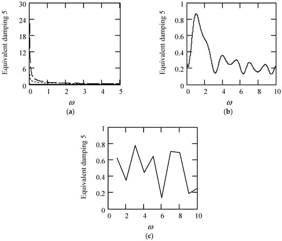
Figure 39.
Plots of ceq5 when k = 1. (a). ceq5 for λ(ω) = 0.9 (solid), 0.6 (dot), 0.3 (dash). (b). ceq5 for λ(ω) = 0.5 + 0.4cos(2ω). (c). ceq5 when λ(ω) is a uniformly distributed random function with the range (0.1, 0.9).
7.2.3. Equivalent Stiffness of Type 5 Multi-Fractional Vibrator
Theorem 46 (Equivalent stiffness 5).
Let keq5 be the equivalent stiffness of a type 5 multi-fractional vibrator. Then,
Proof.
From (124) and (103), we see that the above is valid. This finishes the proof. □
7.2.4. Equivalent Damping Ratio of Type 5 Multi-Fractional Vibrator
Theorem 47 (Equivalent damping ratio 5).
Let ζeq5 be the equivalent damping ratio of a type 5 multi-fractional vibrator. Define it by
Then,
Proof.
Substituting ceq5 and keq5 into (128) produces (129). This finishes the proof. □
Some plots of ζeq5 are indicated in Figure 40.
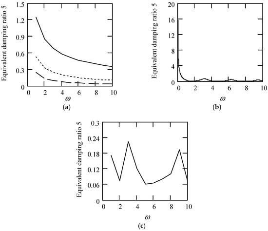
Figure 40.
Plots of ζeq5 when m = 1 and k = 1. (a). ζeq5 for λ(ω) = 0.9 (solid), 0.6 (dot), 0.3 (dash). (b). ζeq5 for λ(ω) = 0.5 + 0.4cos(2ω). (c). ζeq5 when λ(ω) is a uniformly distributed random function with the range (0.1, 0.9).
7.2.5. Equivalent Damping Free Natural Angular Frequency of Type 5 Multi-Fractional Vibrator
Theorem 48 (Equivalent damping free natural angular frequency 5).
Let ωeqn5 be the equivalent damping free natural angular frequency of a type 5 multi-fractional vibrator. Define it by
Then,
Proof.
Substituting keq5 into (130) produces (131). The proof is finished. □
Figure 41 shows some plots of ωeqn5.
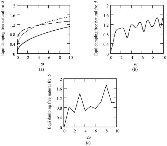
Figure 41.
Plots of ωeqn5 when m = 1 and k = 1. (a). ωeqn5 for λ(ω) = 0.9 (solid), 0.6 (dot), 0.3 (dash). (b). ωeqn5 for λ(ω) = 0.5 + 0.4cos(2ω). (c). ωeqn5 when λ(ω) is a uniformly distributed random function with the range (0.1, 0.9).
7.2.6. Equivalent Damped Natural Angular Frequency of Type 5 Multi-Fractional Vibrator
From the perspective of vibrations, we use |ζeq5| ≤ 1 in what follows. Denote by ωeqd5 the equivalent damped natural angular frequency of a type 5 multi-fractional vibrator. Then,
Theorem 49 (Equivalent damped natural angular frequency 5).
The quantity ωeqd5 is expressed by
Proof.
Substituting ζeq5 and ωeqn5 into (132) yields (133). The proof is finished. □
Figure 42 illustrates some plots of ωeqd5.
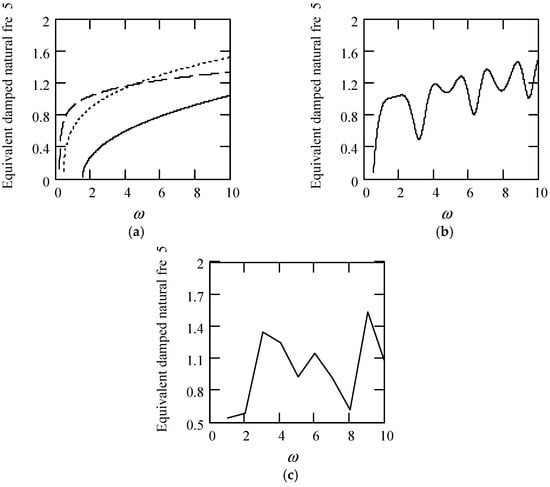
Figure 42.
Plots of ωeqd5 when m = 1 and k = 1. (a). ωeqd5 for λ(ω) = 0.9 (solid), 0.6 (dot), 0.3 (dash). (b). ωeqd5 for λ(ω) = 0.5 + 0.4cos(2ω). (c). ωeqd5 when λ(ω) is a uniformly distributed random function with the range (0.1, 0.9).
7.2.7. Equivalent Frequency Ratio of Type 5 Multi-Fractional Vibrator
Theorem 50 (Equivalent frequency ratio 5).
Let γeq5 be the equivalent frequency ratio of a type 5 multi-fractional vibrator. Define it by
Then,
Proof.
Substituting ωeqn5 into (134) results in (135). This finishes the proof. □
Some plots of γeq5 are shown in Figure 43.
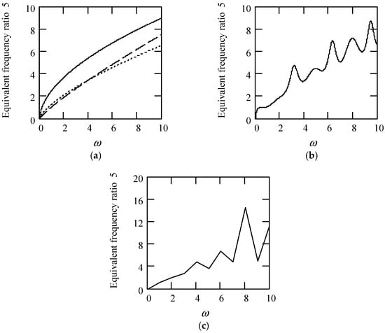
Figure 43.
Plots of γeq5 when m = 1 and k = 1. (a). γeq5 for λ(ω) = 0.9 (solid), 0.6 (dot), 0.3 (dash). (b). γeq5 for λ(ω) = 0.5 + 0.4cos(2ω). (c). γeq5 when λ(ω) is a uniformly distributed random function with the range (0.1, 0.9).
7.3. Frequency Transfer Function of Type 5 Multi-Fractional Vibrator
Theorem 51 (Frequency transfer function 5).
Let H5(ω) be the frequency transfer function in phasor for a type 5 multi-fractional vibrator. It is expressed by
Proof.
Using the notations of ceq5, ζeq5, ωeqn5, and ωeqd5, we write the motion phasor equation of a type 5 multi-fractional vibrator by
Thus,
Substituting ζeq5 and ωeqn5 into the above yields (136). The proof is finished. □
In fact, we can write the motion phasor equation of a type 5 multi-fractional vibrator by
Substituting ceq5 and keq5 into the above also produces (136).
Using γeq5 and ζeq5, we write the above by
The amplitude of H5(ω) is expressed by
The phase of H5(ω) is
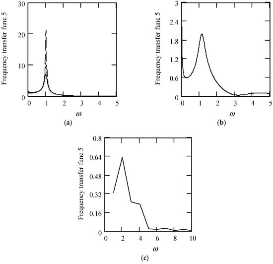
Figure 44.
Plots of |H5(ω)| when m = 1 and k = 1. (a). |H5(ω)| for λ(ω) = 0.09 (solid), 0.06 (dot), 0.03 (dash). (b). |H5(ω)| for λ(ω) = 0.5 + 0.4cos(2ω). (c). |H5(ω)| when λ(ω) is a uniformly distributed random function with the range (0.1, 0.9).
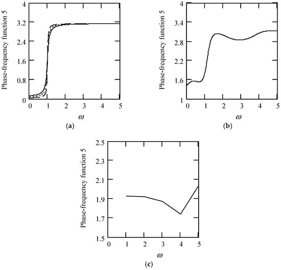
Figure 45.
Plots of φ5(ω) when m = 1 and k = 1. (a). φ5(ω) for λ(ω) = 0.09 (solid), 0.06 (dot), 0.03 (dash). (b). φ5(ω) for λ(ω) = 0.5 + 0.4cos(2ω). (c). φ5(ω) when λ(ω) is a uniformly distributed random function with the range (0.1, 0.9).
7.4. Stationary Response to Sinusoidal Vibration of Type 5 Multi-Fractional Vibrator
Below, we give two expressions of the stationary sinusoidal response to a type 5 multi-fractional vibrator. The stationary sinusoidal response in the phasor domain is expressed by Theorem 52. The one in the time domain is represented by Theorem 53.
Theorem 52 (Response phasor 5).
The response phasor of a type 5 multi-fractional vibrator is given by
Proof.
Because X5 = H5(ω)F, we see that the above is true. The proof is finished. □
The above equation can be written by
Theorem 53 (Stationary sinusoidal response 5).
The stationary sinusoidal response of a type 5 multi-fractional vibrator is given by
Proof.
As x5(t) = Im[X5exp(iωt)], X5 = H5(ω)F, F = F0exp(iθ), and
we have x5(t) = Im{|H5(ω)|F0exp(iωt)exp(iθ)exp[−iφ(ω)]}, which equals to (145). The proof is finished. □
Figure 46 shows some plots of x5(t), demonstrating that there is a noticeable effect of fractional order λ(ω) on the response x5(t).
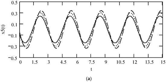
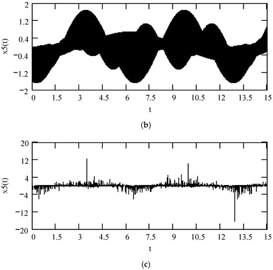
Figure 46.
Plots of x5(t) when ω = 2, F0 = 1, θ = 0, m = 1, and k = 1. (a). x5(t) for λ = 0.9 (solid), λ = 0.6 (dot), λ = 0.3 (dash). (b). x5(t) for λ(ω) = 0.5 + 0.4cos(2ω). (c). x5(t) when λ(ω) is a uniformly distributed random function with the range (0.1, 0.9).
8. Results Regarding Type 6 Multi-Fractional Vibrators
We bring forward the results regarding type 6 multi-fractional vibrators. The motion phasor equation of a type 6 multi-fractional vibrator is presented in Section 8.1. The expressions of equivalent vibration parameters about a type 6 multi-fractional vibrator are described in Section 8.2. The expression of frequency transfer function of a type 6 multi-fractional vibrator is expressed in Section 8.3. The expressions of stationary sinusoidal response to a type 6 multi-fractional vibrator in the phasor domain and the time one are brought forward in Section 8.4.
8.1. Motion Phasor Equation of Type 6 Multi-Fractional Vibrator
Theorem 54 (Motion phasor equation 6).
Let X6 be the phasor of response x6(t) to a type 6 multi-fractional vibrator. Let F be the phasor of excitation f(t) = F0sin(ωt + θ). The motion phasor equation of a type 6 multi-fractional vibrator is given by
Proof.
Using phasor to express both sides of
yields (146). The proof is finished. □
Now, we write the left side of (146) by
When writing the right side of the above by
we have
8.2. Equivalent Parameters of Type 6 Multi-Fractional Vibrator
In Section 8.2, we bring forward the expressions of equivalent vibration parameters of a type 6 multi-fractional vibrator, including equivalent mass in Section 8.2.1, equivalent damping in Section 8.2.2, equivalent stiffness in Section 8.2.3, equivalent damping ratio in Section 8.2.4, equivalent damping free natural angular frequency in Section 8.2.5, equivalent damped natural angular frequency in Section 8.2.6, and equivalent frequency ratio in Section 8.2.7.
8.2.1. Equivalent Mass of Type 6 Multi-Fractional Vibrator
Theorem 55 (Equivalent mass 6).
Denote by meq6 the equivalent mass of a multi-fractional vibrator of type 6. Then,
Proof.
The first item on the right side of (150) stands for an inertia force in the phasor domain. The acceleration in the phasor domain is (iω)2X6. Its coefficient is the equivalent mass. Thus, (151) holds. This finishes the proof. □
Note that
meq6 = meq3.
8.2.2. Equivalent Damping of Type 6 Multi-Fractional Vibrator
Theorem 56 (Equivalent damping 6).
Let ceq6 be the equivalent damping of a type 6 multi-fractional vibrator. Then,
Proof.
The second item on the right side of (150) implies a friction force in the phasor domain. The velocity in the phasor domain is (iω)X6. Its coefficient is the equivalent damping ceq6. Consequently, (153) is valid. The proof is finished. □
Figure 47 illustrates some plots of ceq6.
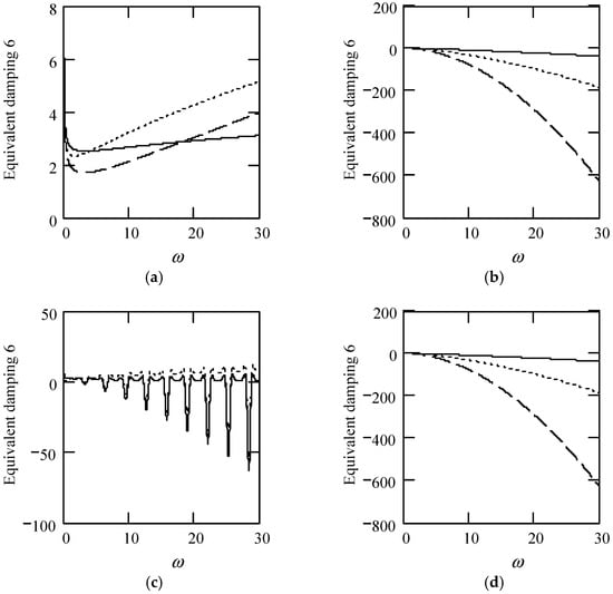
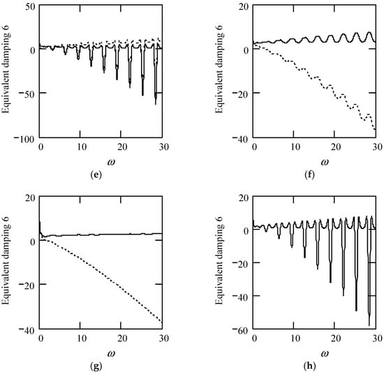
Figure 47.
Plots of ceq6 for m = 1, c = 1, and k = 1. (a). ceq6 with β(ω) = 0.7 and λ(ω) = 0.7 for α(ω) = 1.3 (solid), 1.6 (dot), 1.9 (dash). (b). ceq6 with β(ω) = 0.7 and λ(ω) = 0.7 for α(ω) = 2.3 (solid), 2.6 (dot), 2.9 (dash) (negative damping). (c). ceq6 with β(ω) = 1.3 and λ(ω) = 0.7 for α(ω) = 1.3 (solid), 1.6 (dot), 1.9 (dash). (d). ceq6 with β(ω) = 1.3 and λ(ω) = 0.7 for α(ω) = 2.3 (solid), 2.6 (dot), 2.9 (dash) (negative damping). (e). ceq6 when α(ω) = 1.4 + cos(2ω) and λ(ω) = 0.7 for β(ω) = 0.7 (solid) and β(ω) = 1.3 (dot). (f). ceq6 when β(ω) = 1.2 + 0.5cos(2ω) and λ(ω) = 0.7 for α(ω) = 1.3 (solid), 2.3 (dot). (g). ceq6 when λ(ω) = 0.1 + 0.4cos(2ω) and β(ω) = 0.7 for for α(ω) = 1.3 (solid), 2.3 (dot). (h). ceq6 when α(ω) = 1.4 + cos(2ω), β(ω) = 1.2 + 0.5cos(2ω), and λ(ω) = 0.1 + 0.4cos(2ω).
8.2.3. Equivalent Stiffness of Type 6 Multi-Fractional Vibrator
Theorem 57 (Equivalent stiffness 6).
Let keq6 be the equivalent stiffness of a type 6 multi-fractional vibrator. Then,
Proof.
The third item on the right side of (150) is a restoration force in the phasor domain. The displacement in the phasor domain is X6. Its coefficient is the equivalent stiffness keq6. Therefore, (154) is true. The proof is finished. □
Note that
keq6 = keq5 = keq4.
8.2.4. Equivalent Damping Ratio of Type 6 Multi-Fractional Vibrator
Theorem 58 (Equivalent damping ratio 6).
Denote by ζeq6 the equivalent damping ratio of a type 6 multi-fractional vibrator. Define it by
Then,
Proof.
Substituting meq6, ceq6, and keq6 into (156) yields (157). This finishes the proof. □
Some plots of ζeq6 are indicated in Figure 48.
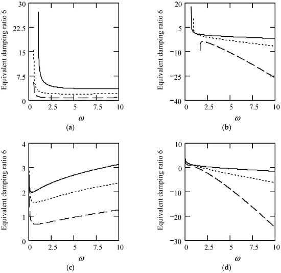
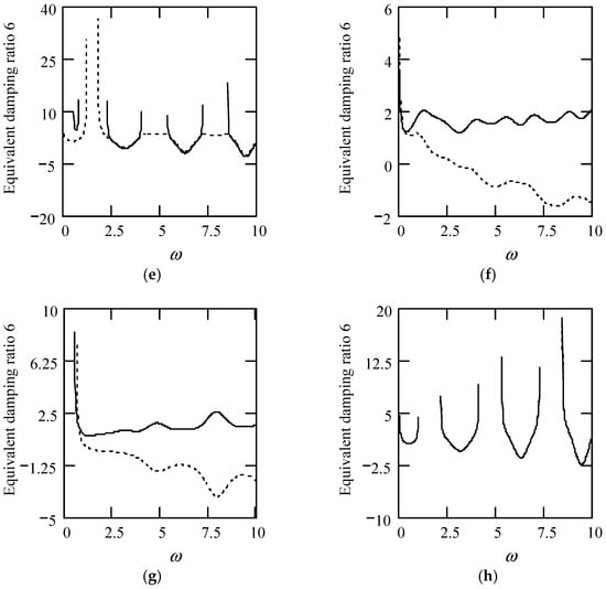
Figure 48.
Plots of ζeq6 for m = 1, c = 1, and k = 1. (a). ζeq6 with β(ω) = 0.7 and λ(ω) = 0.7 for α(ω) = 1.3 (solid), 1.6 (dot), 1.9 (dash). (b). ζeq6 with β(ω) = 0.7 and λ(ω) = 0.7 for α(ω) = 2.3 (solid), 2.6 (dot), 2.9 (dash). (c). ζeq6 with β(ω) = 1.3 and λ(ω) = 0.7 for α(ω) = 1.3 (solid), 1.6 (dot), 1.9 (dash). (d). ζeq6 with β(ω) = 1.3 and λ(ω) = 0.7 for α(ω) = 2.3 (solid), 2.6 (dot), 2.9 (dash). (e). ζeq6 when α(ω) = 1.4 + cos(2ω) and λ(ω) = 0.7 for β(ω) = 0.7 (solid) and β(ω) = 1.3 (dot). (f). ζeq6 when β(ω) = 1.2 + 0.5cos(2ω) and λ(ω) = 0.7 for α(ω) = 1.3 (solid), 2.3 (dot). (g). ζeq6 when λ(ω) = 0.1 + 0.4cos(2ω) and β(ω) = 0.7 for α(ω) = 1.3 (solid), 2.3 (dot). (h). ζeq6 when α(ω) = 1.4 + cos(2ω), β(ω) = 1.2 + 0.5cos(2ω), and λ(ω) = 0.1 + 0.4cos(2ω).
8.2.5. Equivalent Damping Free Natural Angular Frequency of Type 6 Multi-Fractional Vibrator
Theorem 59 (Equivalent damping free natural angular frequency 6).
Denote by ωeqn6 the equivalent damping free natural angular frequency of a type 6 multi-fractional vibrator. It is defined by
Then,
Proof.
Substituting meq6 and keq6 into (158) results in (159). The proof is finished. □
Figure 49 indicates some plots of ωeqn6.
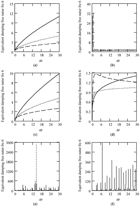
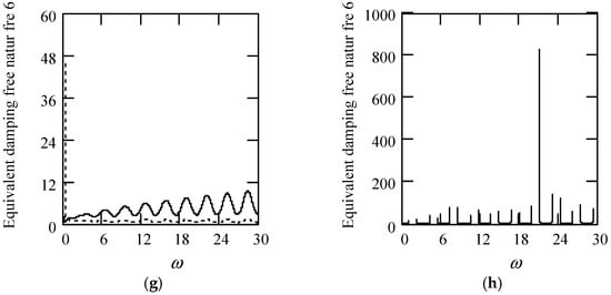
Figure 49.
Plots of ωeqn6 for m = 1, c = 0.2, and k = 1. (a). ωeqn6 with β(ω) = 0.7 and λ(ω) = 0.7 for α(ω) = 1.3 (solid), 1.6 (dot), 1.9 (dash). (b). ωeqn6 with β(ω) = 0.7 and λ(ω) = 0.7 for α(ω) = 2.3 (solid), 2.6 (dot), 2.9 (dash). (c). ωeqn6 with β(ω) = 1.3 and λ(ω) = 0.7 for α(ω) = 1.3 (solid), 1.6 (dot), 1.9 (dash). (d). ωeqn6 with β(ω) = 1.3 and λ(ω) = 0.7 for α(ω) = 2.3 (solid), 2.6 (dot), 2.9 (dash). (e). ωeqn6 when α(ω) = 1.4 + cos(2ω) and λ(ω) = 0.7 for β(ω) = 0.7 (solid) and β(ω) = 1.3 (dot). (f). ωeqn6 when β(ω) = 1.2 + 0.5cos(2ω) and λ(ω) = 0.7 for α(ω) = 1.3 (solid), 2.3 (dot). (g). ωeqn6 when λ(ω) = 0.1 + 0.4cos(2ω) and β(ω) = 0.7 for α(ω) = 1.3 (solid), 2.3 (dot). (h). ωeqn6 when α(ω) = 1.4 + cos(2ω), β(ω) = 1.2 + 0.5cos(2ω), and λ(ω) = 0.1 + 0.4cos(2ω).
8.2.6. Equivalent Damped Natural Angular Frequency of Type 6 Multi-Fractional Vibrator
From a practical perspective of vibrations, |ζeq6| ≤ 1 is used in what follows.
Theorem 60 (Equivalent damped natural angular frequency 6).
Let ωeqd6 be the equivalent damped natural angular frequency of a type 6 multi-fractional vibrator. Define it by
Then,
Proof.
Substituting ζeq6 and ωeqn6 into (160) produces (161). The proof is finished. □
Some plots of ωeqd6 are provided in Figure 50.
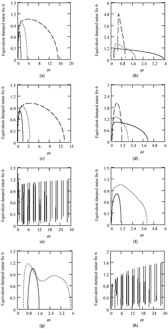
Figure 50.
Plots of ωeqd6 for m = 1, c = 0.2, and k = 1. (a). ωeqd6 with β(ω) = 0.9 and λ(ω) = 0.1 for α(ω) = 1.3 (solid), 1.6 (dot), 1.9 (dash). (b). ωeqd6 with β(ω) = 0.9 and λ(ω) = 0.1 for α(ω) = 2.3 (solid), 2.6 (dot), 2.9 (dash). (c). ωeqd6 with β(ω) = 1.3 and λ(ω) = 0.1 for α(ω) = 1.3 (solid), 1.6 (dot), 1.9 (dash). (d). ωeqd6 with β(ω) = 1.3 and λ(ω) = 0.7 for α(ω) = 2.3 (solid), 2.6 (dot), 2.9 (dash). (e). ωeqd6 when α(ω) = 1.4 + cos(2ω) and λ(ω) = 0.1 for β(ω) = 0.7 (solid) and β(ω) = 1.3 (dot). (f). ωeqd6 when β(ω) = 1.2 + 0.5cos(2ω) and λ(ω) = 0.1 for α(ω) = 1.3 (solid), 2.3 (dot). (g). ωeqd6 when λ(ω) = 0.1 + 0.4cos(2ω) and β(ω) = 0.7 for α(ω) = 1.3 (solid), 2.3 (dot). (h). ωeqd6 when α(ω) = 1.4 + cos(2ω), β(ω) = 1.2 + 0.5cos(2ω), and λ(ω) = 0.1 + 0.4cos(2ω).
8.2.7. Equivalent Frequency Ratio of Type 6 Multi-Fractional Vibrator
Theorem 61 (Equivalent frequency ratio 6).
Denote by γeq6 the equivalent frequency ratio of a type 6 multi-fractional vibrator. Define it by
Then,
Proof.
Substituting ωeqn6 into (162) results in (163). This finishes the proof. □
Figure 51 shows some plots of γeq6.
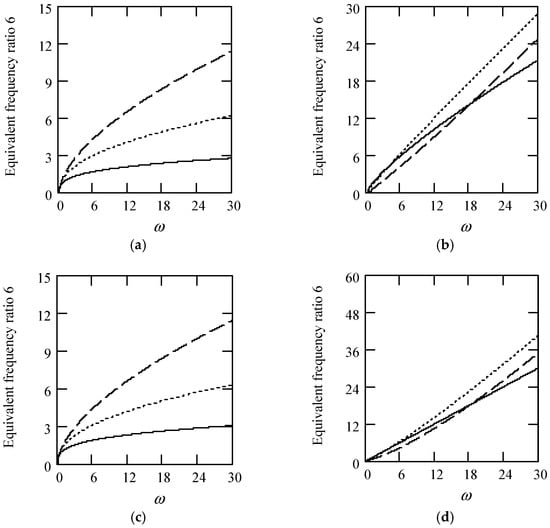
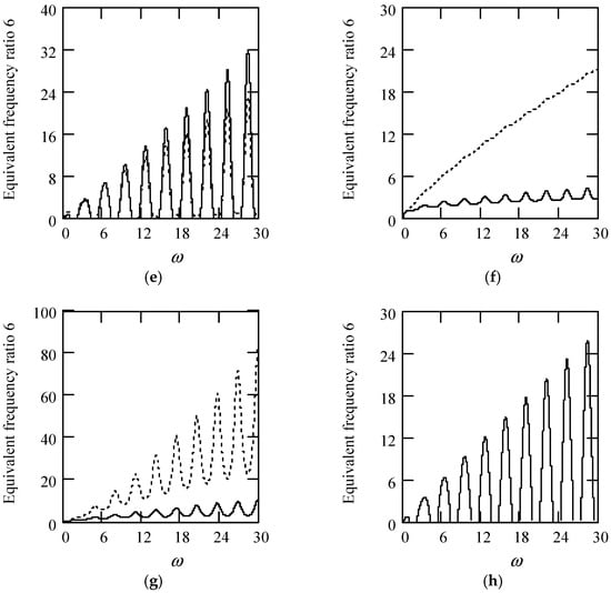
Figure 51.
Plots of γeq6 for m = 1, c = 0.2, and k = 1. (a). γeq6 with β(ω) = 0.7 and λ(ω) = 0.7 for α(ω) = 1.3 (solid), 1.6 (dot), 1.9 (dash). (b). γeq6 with β(ω) = 0.7 and λ(ω) = 0.7 for α(ω) = 2.3 (solid), 2.6 (dot), 2.9 (dash). (c). γeq6 with β(ω) = 1.3 and λ(ω) = 0.7 for α(ω) = 1.3 (solid), 1.6 (dot), 1.9 (dash). (d). γeq6 with β(ω) = 1.3 and λ(ω) = 0.3 for α(ω) = 2.3 (solid), 2.6 (dot), 2.9 (dash). (e). γeq6 when α(ω) = 1.4 + cos(2ω) for λ(ω) = 0.3 and β(ω) = 0.7 (solid) and λ(ω) = 0.7 and β(ω) = 1.3 (dot). (f). γeq6 when β(ω) = 1.2 + 0.5cos(2ω) and λ(ω) = 0.7 for α(ω) = 1.3 (solid), 2.3 (dot). (g). γeq6 when λ(ω) = 0.1 + 0.4cos(2ω) and β(ω) = 0.7 for α(ω) = 1.3 (solid), 2.3 (dot). (h). γeq6 when α(ω) = 1.4 + cos(2ω), β(ω) = 1.2 + 0.5cos(2ω), and λ(ω) = 0.1 + 0.4cos(2ω).
8.3. Frequency Transfer Function of Type 6 Multi-Fractional Vibrator
Theorem 62 (Frequency transfer function 6).
Denote by H6(ω) the frequency transfer function in phasor for a type 6 multi-fractional vibrator. Then,
Proof.
Taking into account the notations of meq6, ceq6, ζeq6, ωeqn6, and ωeqd6, we have the motion phasor equation of a type 6 multi-fractional vibrator in the form
Since H6(ω) = X6/F, we have (164). The proof is finished. □
The amplitude of H6(ω) is
The phase of H6(ω) is
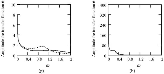
Figure 52.
Plots of |H6(ω)| for m = 1, c = 0.2, and k = 1. (a). |H6(ω)| with β(ω) = 0.7 and λ(ω) = 0.2 for α(ω) = 1.3 (solid), 1.6 (dot), 1.9 (dash). (b). |H6(ω)| with β(ω) = 0.7 and λ(ω) = 0.2 for α(ω) = 2.3 (solid), 2.6 (dot), 2.9 (dash). (c). |H6(ω)| with β(ω) = 1.3 and λ(ω) = 0.2 for α(ω) = 1.3 (solid), 1.6 (dot), 1.9 (dash). (d). |H6(ω)| with β(ω) = 1.3 and λ(ω) = 0.2 for α(ω) = 2.3 (solid), 2.6 (dot), 2.9 (dash). (e). |H6(ω)| when α(ω) = 1.4 + cos(2ω) and λ(ω) = 0.1 for β(ω) = 0.7 (solid) and β(ω) = 1.3 (dot). (f). |H6(ω)| when β(ω) = 1.2 + 0.5cos(2ω) and λ(ω) = 0.1 for α(ω) = 1.3 (solid), 2.3 (dot). (g). |H6(ω)| when λ(ω) = 0.1 + 0.4cos(2ω) and β(ω) = 0.1 for α(ω) = 1.3 (solid), 2.3 (dot). (h). |H6(ω)| when α(ω) = 1.4 + cos(2ω), β(ω) = 1.2 + 0.5cos(2ω), and λ(ω) = 0.1 + 0.4cos(2ω).
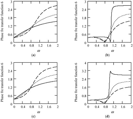
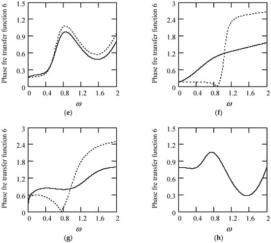
Figure 53.
Plots of φ6(ω) for m = 1, c = 0.2, and k = 1. (a). φ6(ω) with β(ω) = 0.7 and λ(ω) = 0.2 for α(ω) = 1.3 (solid), 1.6 (dot), 1.9 (dash). (b). φ6(ω) with β(ω) = 0.7 and λ(ω) = 0.2 for α(ω) = 2.3 (solid), 2.6 (dot), 2.9 (dash). (c). φ6(ω) with β(ω) = 1.3 and λ(ω) = 0.2 for α(ω) = 1.3 (solid), 1.6 (dot), 1.9 (dash). (d). φ6(ω) with β(ω) = 1.3 and λ(ω) = 0.2 for α(ω) = 2.3 (solid), 2.6 (dot), 2.9 (dash). (e). φ6(ω) when α(ω) = 1.4 + cos(2ω) and λ(ω) = 0.1 for β(ω) = 0.7 (solid) and β(ω) = 1.3 (dot). (f). φ6(ω) when β(ω) = 1.2 + 0.5cos(2ω) and λ(ω) = 0.1 for α(ω) = 1.3 (solid), 2.3 (dot). (g). φ6(ω) when λ(ω) = 0.1 + 0.4cos(2ω) and β(ω) = 0.1 for α(ω) = 1.3 (solid), 2.3 (dot). (h). φ6(ω) when α(ω) = 1.4 + cos(2ω), β(ω) = 1.2 + 0.5cos(2ω), and λ(ω) = 0.1 + 0.4cos(2ω).
8.4. Stationary Response to Sinusoidal Vibration of Type 6 Multi-Fractional Vibrator
In Section 8.4, we give two expressions of the stationary sinusoidal response to a type 6 multi-fractional vibrator. The one in Theorem 63 is the response in the phasor domain and the other in Theorem 64 is one in the time domain.
Theorem 63 (Response phasor 6).
The response phasor of a type 6 multi-fractional vibrator is in the form
Proof.
Because X6 = H6(ω)F, the above is true. The proof is finished. □
Theorem 64 (Stationary sinusoidal response 6).
The stationary sinusoidal response of a type 6 multi-fractional vibrator is in the form
Proof.
Due to x6(t) = Im[X6exp(iωt)], X6 = H6(ω)F, F = F0exp(iθ), and
we have x6(t) = Im{|H6(ω)|F0exp(iωt)exp(iθ)exp[−iφ(ω)]}, which equals to (169). The proof is finished. □
Figure 54 indicates some plots of x6(t) for different values of α, β, and λ. It demonstrates that there is a considerable effect of fractional orders α(ω), β(ω), and λ(ω) on x6(t).
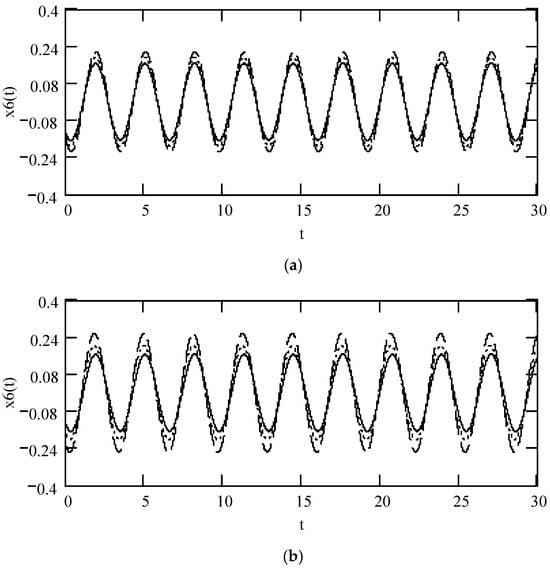
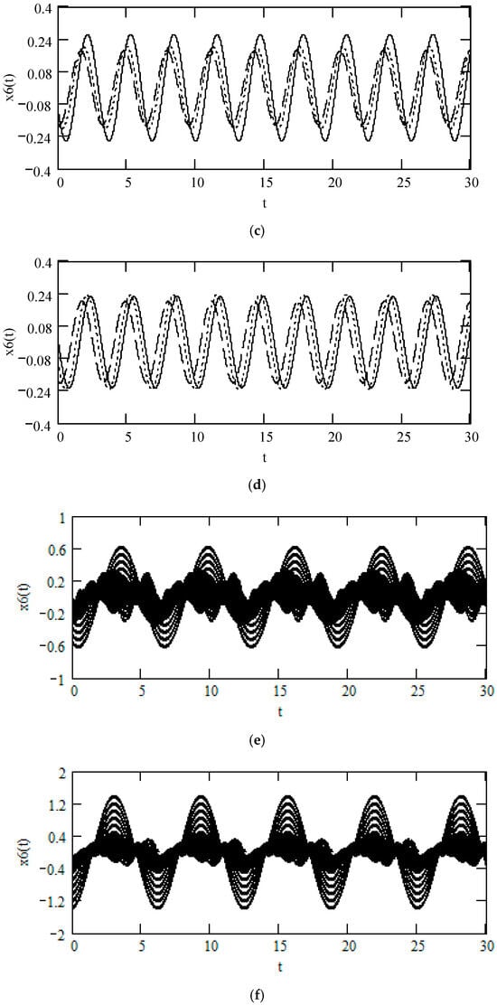
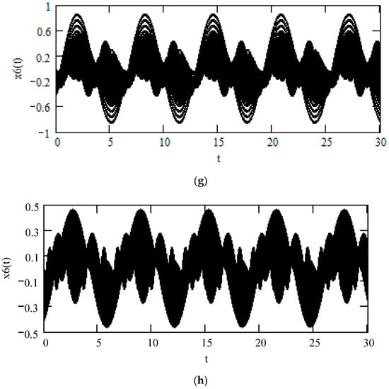
Figure 54.
Plots of x6(t) when ω = 2, F0 = 1, θ = 0, m = 1, c = 1, and k = 1. (a). x6(t) when α = 1.8, β = 1.2, for λ = 0.8 (solid), λ = 0.5 (dot), λ = 0.2 (dash). (b). x6(t) for α = 1.8, λ = 0.8 for β = 1.2 (solid), 0.8 (dot), 0.4 (dash). (c). x6(t) for β = 0.8, λ = 0.8 for α = 2.2 (solid), α = 1.8 (dot), α = 1.4 (dash). (d). x6(t) when β(ω) = 1.3 and λ(ω) = 0.2 for α(ω) = 2.3 (solid), 2.6 (dot), 2.9 (dash). (e). when α(ω) = 1.4 + cos(2ω) and λ(ω) = 0.1 for β(ω) = 0.7 (solid) and β(ω) = 1.3 (dot). (f). x6(t) when β(ω) = 1.2 + 0.5cos(2ω) and λ(ω) = 0.1 for α(ω) = 1.3 (solid), 2.3 (dot). (g). x6(t) when λ(ω) = 0.1 + 0.4cos(2ω) and β(ω) = 0.1 for α(ω) = 1.3 (solid), 2.3 (dot). (h). x6(t) when α(ω) = 1.4 + cos(2ω), β(ω) = 1.2 + 0.5cos(2ω), and λ(ω) = 0.1 + 0.4cos(2ω).
9. Results Regarding Type 7 Multi-Fractional Vibrators
We propose the results with respect to type 7 multi-fractional vibrators as follows. The motion phasor equation of a type 7 multi-fractional vibrator is presented in Section 9.1. The expressions of equivalent vibration parameters about a type 7 multi-fractional vibrator are given in Section 9.2. The expression of frequency transfer function of a type 7 multi-fractional vibrator is in Section 9.3. The expressions of stationary sinusoidal response to a type 7 multi-fractional vibrator in the phasor domain and the time one are presented in Section 9.4.
9.1. Motion Phasor Equation of Type 7 Multi-Fractional Vibrator
Theorem 65 (Motion phasor equation 7).
Let X7 be the phasor of response x7(t) to a type 7 multi-fractional vibrator. Let F be the phasor of excitation f(t) = F0sin(ωt + θ). The motion phasor equation of a type 7 multi-fractional vibrator is given by
Proof.
Using phasor to express both sides of
results in (170). This finishes the proof. □
With the principal branches of iβ and iλ, the left side of the above equation is given by
Writing the right side of the above by
yields
9.2. Equivalent Parameters of Type 7 Multi-Fractional Vibrator
We put forward the expressions of equivalent vibration parameters of a type 7 multi-fractional vibrator in Section 9.2 below. They are equivalent mass in Section 9.2.1, equivalent damping in Section 9.2.2, equivalent stiffness in Section 9.2.3, equivalent damping ratio in Section 9.2.4, equivalent damping free natural angular frequency in Section 9.2.5, equivalent damped natural angular frequency in Section 9.2.6, and equivalent frequency ratio in Section 9.2.7.
9.2.1. Equivalent Mass of Type 7 Multi-Fractional Vibrator
Theorem 66 (Equivalent mass 7).
Denote by meq7 the equivalent mass of a multi-fractional vibrator of type 7. Then,
Proof.
The first item on the right side of (174) stands for an inertia force in the phasor domain. The acceleration in the phasor domain is (iω)2X7. Its coefficient is the equivalent mass. Thus, (175) is true. This finishes the proof. □
Note that
meq7 = meq2.
9.2.2. Equivalent Damping of Type 7 Multi-Fractional Vibrator
Theorem 67 (Equivalent damping 7).
Let ceq7 be the equivalent damping of a type 7 multi-fractional vibrator. Then,
Proof.
The second item on the right side of (174) implies a friction force in the phasor domain. The velocity in the phasor domain is (iω)X7. Its coefficient is the equivalent damping ceq7. Consequently, (177) holds. The proof is finished. □
Figure 55 illustrates some plots of ceq7.
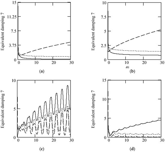
Figure 55.
Plots of ceq7 for m = 1, c = 1, and k = 1. (a). ceq7 with β(ω) = 0.3 (solid), 0.9 (dot), 1.6 (dash) for λ(ω) = 0.7. (b). ceq7 with β(ω) = 0.3 (solid), 0.9 (dot), 1.6 (dash) for λ(ω) = 0.9. (c). ceq7 when β(ω) = 1.2 + 0.5cos(2ω) and λ(ω) = 1.6 (solid), 0.9 (dot), 0.3 (dash). (d). ceq7 when λ(ω) = 0.1 + 0.4cos(2ω) for β(ω) 1.6 (solid), 0.9 (dot), 0.3 (dash).
9.2.3. Equivalent Stiffness of Type 7 Multi-Fractional Vibrator
Theorem 68 (Equivalent stiffness 7).
Let keq7 be the equivalent stiffness of a type 7 multi-fractional vibrator. Then,
Proof.
The third item on the right side of (174) is a restoration force in the phasor domain. The displacement in the phasor domain is X6. Its coefficient is the equivalent stiffness keq7. Therefore, (178) is true. This finishes the proof. □
Note that
keq7 = keq6 = keq5 = keq4.
9.2.4. Equivalent Damping Ratio of Type 7 Multi-Fractional Vibrator
Theorem 69 (Equivalent damping ratio 7).
Denote by ζeq7 the equivalent damping ratio of a type 7 multi-fractional vibrator. Define it by
Then,
Proof.
Substituting meq7, ceq7, and keq7 into (180) results in (181). The proof is finished. □
Some plots of ζeq7 are indicated in Figure 56.
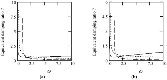
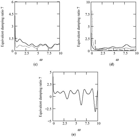
Figure 56.
Plots of ζeq7 for m = 1, c = 1, and k = 1. (a). ζeq7 with β(ω) = 1.6 (solid), 0.9 (dot), 0.3 (dash) for λ(ω) = 0.7. (b). ζeq7 with β(ω) = 1.6 (solid), 0.9 (dot), 0.3 (dash) for λ(ω) = 0.2. (c). ζeq7 when β(ω) = 1.2 + 0.5cos(2ω) for λ(ω) = 0.7 (solid), 0.2 (dot). (d). ζeq7 when λ(ω) = 0.1 + 0.4cos(2ω) for β(ω) = 1.6 (solid), 0.9 (dot), 0.3 (dot). (e). ζeq7 when β(ω) = 1.2 + 0.5cos(2ω) and λ(ω) = 0.1 + 0.4cos(2ω).
9.2.5. Equivalent Damping Free Natural Angular Frequency of Type 7 Multi-Fractional Vibrator
Theorem 70 (Equivalent damping free natural angular frequency 7).
Denote by ωeqn7 the equivalent damping free natural angular frequency of a type 7 multi-fractional vibrator. Define it by
Then,
Proof.
Substituting meq7 and keq7 into (182) yields (183). The proof is finished. □
Figure 57 indicates some plots of ωeqn7.
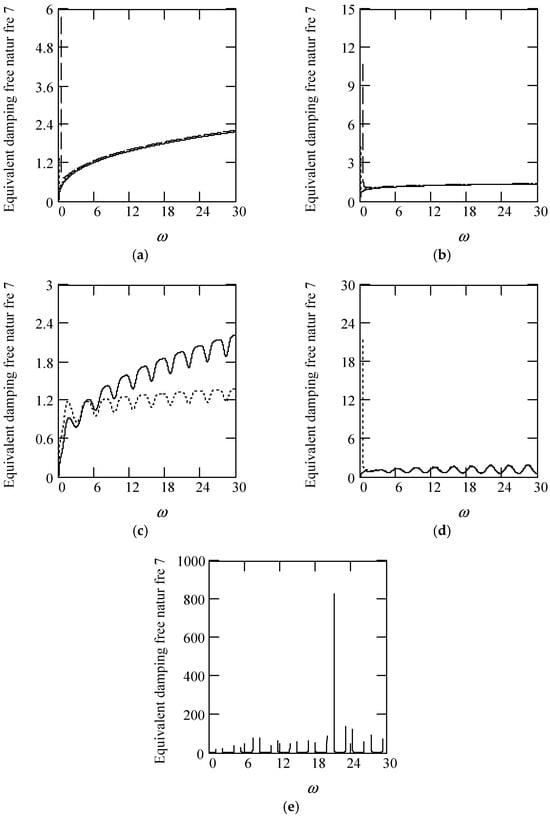
Figure 57.
Plots of ωeqn7 for m = 1, c = 0.2, and k = 1. (a). ωeqn7 with β(ω) = 1.6 (solid), 0.9 (dot), 0.3 (dash) for λ(ω) = 0.7. (b). ωeqn7 with β(ω) = 1.6 (solid), 0.9 (dot), 0.3 (dash) for λ(ω) = 0.2. (c). ωeqn6 when β(ω) = 1.2 + 0.5cos(2ω) for λ(ω) = 0.7 (solid), 0.2 (dot). (d). ωeqn6 when λ(ω) = 0.1 + 0.4cos(2ω) for β(ω) = 1.8 (solid), 0.2 (dot). (e). ωeqn7 when β(ω) = 1.2 + 0.5cos(2ω) and λ(ω) = 0.1 + 0.4cos(2ω).
9.2.6. Equivalent Damped Natural Angular Frequency of Type 7 Multi-Fractional Vibrator
From a practical perspective of vibrations, |ζeq7| ≤ 1 is used in what follows.
Theorem 71 (Equivalent damped natural angular frequency 7).
Let ωeqd7 be the equivalent damped natural angular frequency of a type 7 multi-fractional vibrator. Define it by
Then,
Proof.
Substituting ζeq7 and ωeqn7 into (184) yields (185). This finishes the proof. □
Some plots of ωeqd7 are shown in Figure 58.
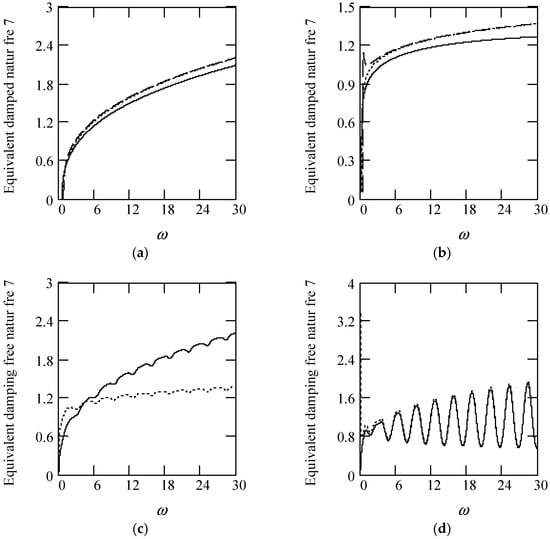
Figure 58.
Plots of ωeqd7 for m = 1, c = 0.2, and k = 1. (a). ωeqd7 with β(ω) = 1.6 (solid), 0.9 (dot), 0.3 (dash) for λ(ω) = 0.7. (b). ωeqd7 with β(ω) = 1.6 (solid), 0.9 (dot), 0.3 (dash) for λ(ω) = 0.2. (c). ωeqd7 when β(ω) = 1.2 + 0.5cos(2ω) for λ(ω) = 0.7 (solid), 0.2 (dot). (d). ωeqd7 when λ(ω) = 0.1 + 0.4cos(2ω) for β(ω) = 1.6 (solid), 0.8 (dot).
9.2.7. Equivalent Frequency Ratio of Type 7 Multi-Fractional Vibrator
Theorem 72 (Equivalent frequency ratio 7).
Denote by γeq7 the equivalent frequency ratio of a type 7 multi-fractional vibrator. Define it by
Then,
Proof.
Substituting ωeqn7 into (186) yields (187). The proof is finished. □
Figure 59 shows some plots of γeq7.
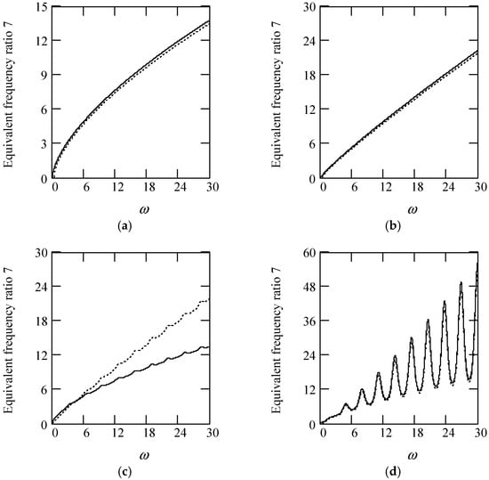
Figure 59.
Plots of γeq7 for m = 1, c = 0.2, and k = 1. (a). γeq7 with β(ω) = 1.6 (solid), 0.3 (dot) for λ(ω) = 0.7. (b). γeq7 with β(ω) = 1.6 (solid), 0.3 (dot) for λ(ω) = 0.2. (c). γeq7 when β(ω) = 1.2 + 0.5cos(2ω) for λ(ω) = 0.7 (solid), 0.2 (dot). (d). γeq7 when λ(ω) = 0.1 + 0.4cos(2ω) for β(ω) = 1.9 (solid), 0.1 (dot).
9.3. Frequency Transfer Function of Type 7 Multi-Fractional Vibrator
Theorem 73 (Frequency transfer function 7).
Let H7(ω) be the frequency transfer function in phasor for a type 7 multi-fractional vibrator. Then,
Proof.
Considering meq7, ceq7, ζeq7, ωeqn7, and ωeqd7, we write the motion phasor equation of a type 7 multi-fractional vibrator in the form
Owing to H7(ω) = X7/F, we have (188). This finishes the proof. □
|H7(ω)| is expressed by
The phase of H7(ω) is
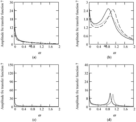
Figure 60.
Plots of |H7(ω)| for m = 1, c = 0.2, and k = 1. (a). |H7(ω)| with β(ω) = 1.6 (solid), 0.9 9 (dot), 0.3 (dash) for λ(ω) = 0.7. (b). |H7(ω)| with β(ω) = 1.6 (solid), 0.9 9 (dot), 0.3 (dash) for λ(ω) = 0.2. (c). |H7(ω)| when β(ω) = 1.2 + 0.5cos(2ω) for λ(ω) = 0.7 (solid), 0.2 (dot). (d). |H7(ω)| when λ(ω) = 0.1 + 0.4cos(2ω) for β(ω) = 1.6 (solid), 0.3 (dot).
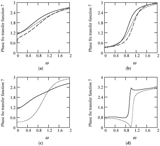
Figure 61.
Plots of φ7(ω) for m = 1, c = 0.2, and k = 1. (a). φ7(ω) with β(ω) = 1.6 (solid), 0.9 (dot), 0.3 (dash) for λ(ω) = 0.7. (b). φ7(ω) with β(ω) = 1.6 (solid), 0.9 (dot), 0.3 (dash) for λ(ω) = 0.2. (c). φ7(ω) when β(ω) = 1.2 + 0.5cos(2ω) for λ(ω) = 0.7 (solid), 0.2 (dot). (d). φ7(ω) when λ(ω) = 0.1 + 0.4cos(2ω) for β(ω) = 0.1 for α(ω) = 1.3 (solid), 2.3 (dot).
9.4. Stationary Response to Sinusoidal Vibration of Type 7 Multi-Fractional Vibrator
In Section 9.4, we bring forward two expressions of stationary sinusoidal response to a type 7 multi-fractional vibrator. Theorem 74 gives the expression of the response in the phasor domain while Theorem 75 the one in the time domain.
Theorem 74 (Response phasor 7).
The response phasor of a type 7 multi-fractional vibrator is in the form
Proof.
Due to X7 = H7(ω)F, the above is valid. This finishes the proof. □
Theorem 75 (Stationary sinusoidal response 7).
The stationary sinusoidal response of a type 7 multi-fractional vibrator is in the form
Proof.
Since x7(t) = Im[X7exp(iωt)], X7 = H7(ω)F, F = F0exp(iθ), and
we have x7(t) = Im{|H7(ω)|F0exp(iωt)exp(iθ)exp[−iφ(ω)]}. Thus, (193) is true. The proof is finished. □
Figure 62 indicates some plots of x7(t) for different values of β(ω) and λ(ω). It demonstrates that there is a considerable effect of fractional orders β(ω) and λ(ω) on x7(t).
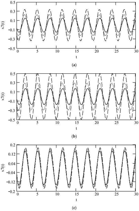
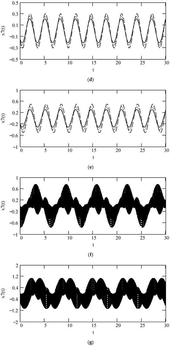
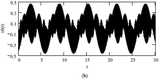
Figure 62.
Plots of x7(t) when ω = 2, F0 = 1, θ = 0, m = 1, c = 1, and k = 1. (a). x7(t) when β(ω) = 1.6 (solid), 0.9 (dot), 0.3 (dash) for λ(ω) = 0.7. (b). x7(t) when β(ω) = 1.6 (solid), 0.9 (dot), 0.3 (dash) for λ(ω) = 0.2. (c). x7(t) for β(ω) = 1.6, λ(ω) = 0.8 (solid), 0.5 (dot), 0.1 (dash). (d). x7(t) when β(ω) = 0.9, λ(ω) = 0.8 (solid), 0.5 (dot), 0.1 (dash). (e). x7(t) when β(ω) = 0.3, λ(ω) = 0.8 (solid), 0.5 (dot), 0.1 (dash). (f). x7(t) when β(ω) = 1.2 + 0.5cos(2ω) for λ(ω) = 0.7 (solid), 0.2 (dot). (g). x7(t) when λ(ω) = 0.1 + 0.4cos(2ω) for β(ω) = 1.5 (solid), 0.5 (dot). (h). x7(t) when β(ω) = 1.2 + 0.5cos(2ω) and λ(ω) = 0.1 + 0.4cos(2ω).
10. Discussions
With respect to seven types of multi-fractional vibrators, the expressions of equivalent parameters (mass, damping, stiffness, damping ratio, damping free natural angular frequency, damped natural angular frequency, frequency ratio) and frequency transfer functions in this paper are the same as those in the author’s previous work [,,]. However, the methods deriving these expressions are different. Those in [,,] are based on Fourier transform but this research uses multi-fractional phasor. Note that the concept and expression of the multi-fractional phasor are new in the field. Moreover, the present analytic expressions of stationary sinusoidal responses to seven types of multi-fractional vibrators are novel.
There are research issues with respect to seven types of multi-fractional vibrators in addition to the stationary sinusoidal responses addressed previously. There are two topics we are interested in examining in the future. One is to study what analytical expressions of −3dB frequency bandwidth are with respect to seven types of multi-fractional vibrators. The other is to explore identification methods of structures with seven types of multi-fractional vibrators.
11. Conclusions and Summary
We have introduced the multi-fractional phasor in Theorem 1. The motion phasor equations of seven types of multi-fractional vibrators are put forward in Theorems 2, 12, 22, 32, 43, 54, and 65, respectively. The analytical expressions of response phasors of seven types of multi-fractional vibrators are presented in Theorems 10, 20, 30, 41, 52, 63, and 74, respectively. The expressions of the stationary sinusoidal responses of seven types of multi-fractional vibration systems are analytically proposed in Theorems 11, 21, 31, 42, 53, 64, and 75, respectively. In addition, based on multi-fractional phasor, we have obtained the following results.
- The analytical expressions of equivalent masses of seven types of multi-fractional vibrators, which are given by Theorems 3, 13, 23, 33, 44, 55, and 66, respectively.
- The analytical expressions of equivalent dampings of seven types of multi-fractional vibrators, which are, respectively, represented by Theorems 4, 14, 24, 34, 45, 56, and 67.
- The analytical expressions of equivalent damping ratios of seven types of multi-fractional vibrators, which are expressed in Theorems 5, 15, 25, 36, 47, 58, and 69, respectively.
- The analytical expressions of equivalent stiffnesses of types 4–7 multi-fractional vibrators, which are, respectively, presented by Theorems 35, 46, 57, and 68.
- The analytical expressions of equivalent damping free natural angular frequencies of seven types of multi-fractional vibrators, which are, respectively, given by Theorems 6, 16, 26, 37, 48, 59, and 70.
- Equivalent damped free natural angular frequencies of seven types of multi-fractional vibrators, which are, respectively, described in Theorems 7, 17, 27, 38, 49, 60, and 71.
- The analytical expressions of equivalent frequency ratios of seven types of multi-fractional vibrators, which are explained in Theorems 8, 18, 28, 39, 50, 61, and 72, respectively.
- The analytical expressions of frequency transfer functions of seven types of multi-fractional vibrators, which are addressed in Theorems 9, 19, 29, 40, 51, 62, and 73, respectively.
The effects of multi-fractional orders on stationary sinusoidal responses of those multi-fractional vibrators are noticeable.
Funding
This research received no external funding.
Data Availability Statement
Data are contained within the article.
Conflicts of Interest
The author declares no conflict of interest.
References
- Uchaikin, V.V. Fractional Derivatives for Physicists and Engineers; Springer: Berlin/Heidelberg, Germany, 2013. [Google Scholar]
- Duan, J.-S. The Periodic Solution of Fractional Oscillation Equation with Periodic Input. Adv. Math. Phys. 2013, 2013, 869484. [Google Scholar] [CrossRef]
- Duan, J.-S.; Wang, Z.; Liu, Y.-L.; Qiu, X. Eigenvalue problems for fractional ordinary differential equations. Chaos Solitons Fractals 2013, 46, 46–53. [Google Scholar] [CrossRef]
- Duan, J.-S.; Hu, D.-C. Vibration Systems with Fractional-Order and Distributed-Order Derivatives Characterizing Viscoinertia. Fractal Fract. 2021, 5, 67. [Google Scholar] [CrossRef]
- Pskhu, A.V.; Rekhviashvili, S.S. Analysis of Forced Oscillations of a Fractional Oscillator. Tech. Phys. Lett. 2018, 44, 1218–1221. [Google Scholar] [CrossRef]
- Zelenev, V.M.; Meshkov, S.I.; Rossikhin, Y.A. Damped vibrations of hereditary -elastic systems with weakly singular kernels. J. Appl. Mech. Tech. Phys. 1970, 11, 290–293. [Google Scholar] [CrossRef]
- Freundlich, J. Vibrations of a simply supported beam with a fractional derivative order viscoelastic material model—Supports movement excitation. Shock. Vib. 2013, 20, 126735. [Google Scholar]
- Freundlich, J. Transient vibrations of a fractional Kelvin-Voigt viscoelastic cantilever beam with a tip mass and subjected to a base excitation. J. Sound Vib. 2018, 438, 99–115. [Google Scholar] [CrossRef]
- Al-Rabtah, A.; Ertürk, V.S.; Momani, S. Solutions of a fractional oscillator by using differential transform method. Comput. Math. Appl. 2010, 59, 1356–1362. [Google Scholar] [CrossRef]
- Zurigat, M. Solving fractional oscillators using Laplace homotopy analysis method. Ann. Univ. Craiova Math. Comput. Sci. Ser. 2011, 38, 4. [Google Scholar]
- Blaszczyk, T. A numerical solution of a fractional oscillator equation in a non-resisting medium with natural boundary conditions. Rom. Rep. Phys. 2015, 67, 350–358. [Google Scholar]
- Blaszczyk, T.; Ciesielski, M. Fractional oscillator equation—Transformation into integral equation and numerical solution. Appl. Math. Comput. 2015, 257, 428–435. [Google Scholar] [CrossRef]
- Blaszczyk, T.; Ciesielski, M.; Klimek, M.; Leszczynski, J. Numerical solution of fractional oscillator equation. Appl. Math. Comput. 2011, 218, 2480–2488. [Google Scholar] [CrossRef]
- Achar, B.N.N.; Hanneken, J.W.; Clarke, T. Damping characteristics of a fractional oscillator. Phys. A 2004, 339, 311–319. [Google Scholar] [CrossRef]
- Achar, B.N.; Hanneken, J.W.; Clarke, T. Response characteristics of a fractional oscillator. Phys. A Stat. Mech. Its Appl. 2002, 309, 275–288. [Google Scholar] [CrossRef]
- Achar, B.; Hanneken, J.; Enck, T.; Clarke, T. Dynamics of the fractional oscillator. Phys. A Stat. Mech. Its Appl. 2001, 297, 361–367. [Google Scholar] [CrossRef]
- Rossikhin, Y.A.; Shitikova, M.V. Analysis of the Viscoelastic Rod Dynamics via Models Involving Fractional Derivatives or Operators of Two different Orders. Shock. Vib. Dig. 2004, 36, 3–26. [Google Scholar] [CrossRef]
- Rossikhin, Y.A.; Shitikova, M.V. Application of Fractional Calculus for Dynamic Problems of Solid Mechanics: Novel Trends and Recent Results. Appl. Mech. Rev. 2010, 63, 010801. [Google Scholar] [CrossRef]
- Rossikhin, Y.A.; Shitikova, M. Application of Fractional Operators to the Analysis of Damped Vibrations of Viscoelastic Single-Mass Systems. J. Sound Vib. 1997, 199, 567–586. [Google Scholar] [CrossRef]
- Rossikhin, Y.A.; Shitikova, M.V. Classical beams and plates in a fractional derivative medium, Impact response. In Encyclopedia of Continuum Mechanics; Springer: Berlin/Heidelberg, Germany, 2020; Volume 1, pp. 294–305. [Google Scholar]
- Rossikhin, Y.A. Reflections on Two Parallel Ways in the Progress of Fractional Calculus in Mechanics of Solids. Appl. Mech. Rev. 2010, 63, 010701. [Google Scholar] [CrossRef]
- Shitikova, M.V. Impact response of a thin shallow doubly curved linear viscoelastic shell rectangular in plan. Math. Mech. Solids 2022, 27, 1721–1739. [Google Scholar] [CrossRef]
- Shitikova, M.V. Fractional Operator Viscoelastic Models in Dynamic Problems of Mechanics of Solids: A Review. Mech. Solids 2022, 57, 1–33. [Google Scholar] [CrossRef]
- Shitikova, M.; Kandu, V.; Krusser, A. On nonlinear vibrations of an elastic plate on a fractional viscoelastic foundation in a viscoelastic medium in the presence of the one-to-one internal resonance. J. Sound Vib. 2023, 549, 117564. [Google Scholar] [CrossRef]
- El-Nabulsi, R.A.; Anukool, W. Vlasov equation, waves and dispersion relations in fractal dimensions: Landau damping and the toroidal ion temperature gradient instability problem. Waves Random Complex Media 2022. [Google Scholar] [CrossRef]
- Liu, Q.X.; Liu, J.K.; Chen, Y.M. A Second-Order Scheme for Nonlinear Fractional Oscillators Based on Newmark-β Algorithm. J. Comput. Nonlinear Dyn. 2018, 13, 084501. [Google Scholar] [CrossRef]
- Sofi, A. Nonlinear vibrations of beams with fractional derivative elements crossed by moving loads. Int. J. Non-Linear Mech. 2024, 159, 104567. [Google Scholar] [CrossRef]
- Li, M. Three Classes of Fractional Oscillators. Symmetry 2018, 10, 40. [Google Scholar] [CrossRef]
- Li, M. PSD and cross PSD of responses of seven classes of fractional vibrations driven by fGn, fBm, fractional OU process, and von Kármán process. Symmetry 2024, 16, 635. [Google Scholar] [CrossRef]
- Li, M. Fractional Vibrations with Applications to Euler-Bernoulli Beams; CRC Press: Boca Raton, UK, 2023. [Google Scholar]
- Drozdov, A. Fractional oscillator driven by a Gaussian noise. Phys. A Stat. Mech. Its Appl. 2007, 376, 237–245. [Google Scholar] [CrossRef]
- Stanislavsky, A.A. Fractional oscillator. Phys. Rev. E 2004, 70, 051103. [Google Scholar] [CrossRef]
- Tofighi, A. The intrinsic damping of the fractional oscillator. Phys. A Stat. Mech. Its Appl. 2003, 329, 29–34. [Google Scholar] [CrossRef]
- Ryabov, Y.E.; Puzenko, A. Damped oscillations in view of the fractional oscillator equation. Phys. Rev. B 2002, 66, 184201. [Google Scholar] [CrossRef]
- Ahmad, W.; El-Khazali, R.; Elwakil, A. Fractional-order Wien-bridge oscillator. Electron. Lett. 2001, 37, 1110. [Google Scholar] [CrossRef]
- Tavazoei, M.S. Reduction of oscillations via fractional order pre-filtering. Signal Process. 2015, 107, 407–414. [Google Scholar] [CrossRef]
- Sandev, T.; Tomovski, Ž. The general time fractional wave equation for a vibrating string. J. Phys. A Math. Theor. 2010, 43, 055204. [Google Scholar] [CrossRef]
- Singh, H.; Srivastava, H.; Kumar, D. A reliable numerical algorithm for the fractional vibration equation. Chaos Solitons Fractals 2017, 103, 131–138. [Google Scholar] [CrossRef]
- Eab, C.H.; Lim, S. Path integral representation of fractional harmonic oscillator. Phys. A Stat. Mech. Its Appl. 2006, 371, 303–316. [Google Scholar] [CrossRef]
- Lin, L.-F.; Chen, C.; Zhong, S.-C.; Wang, H.-Q. Stochastic Resonance in a Fractional Oscillator with Random Mass and Random Frequency. J. Stat. Phys. 2015, 160, 497–511. [Google Scholar] [CrossRef]
- Duan, J.-S. A Modified Fractional Derivative and its Application to Fractional Vibration Equation. Appl. Math. Inf. Sci. 2016, 10, 1863–1869. [Google Scholar] [CrossRef]
- Alkhaldi, H.S.; Abu-Alshaikh, I.M.; Al-Rabadi, A.N. Vibration control of fractionally-damped beam subjected to a moving vehicle and attached to fractionally-damped multi-absorbers. Adv. Math. Phys. 2013, 2013, 232160. [Google Scholar] [CrossRef]
- Dai, H.; Zheng, Z.; Wang, W. On generalized fractional vibration equation. Chaos Solitons Fractals 2017, 95, 48–51. [Google Scholar] [CrossRef]
- Ren, R.; Luo, M.; Deng, K. Stochastic resonance in a fractional oscillator driven by multiplicative quadratic noise. J. Stat. Mech. Theory Exp. 2017, 2017, 023210. [Google Scholar] [CrossRef]
- Xu, Y.; Li, Y.; Liu, D.; Jia, W.; Huang, H. Responses of Duffing oscillator with fractional damping and random phase. Nonlinear Dyn. 2013, 74, 745–753. [Google Scholar] [CrossRef]
- He, G.; Tian, Y.; Wang, Y. Stochastic resonance in a fractional oscillator with random damping strength and random spring stiffness. J. Stat. Mech. Theory Exp. 2013, 2013, P09026. [Google Scholar] [CrossRef]
- Leung, A.; Guo, Z.; Yang, H. Fractional derivative and time delay damper characteristics in Duffing–van der Pol oscillators. Commun. Nonlinear Sci. Numer. Simul. 2013, 18, 2900–2915. [Google Scholar] [CrossRef]
- Chen, L.; Zhuang, Q.; Zhu, W. Response of SDOF nonlinear oscillators with lightly fractional derivative damping under real noise excitations. Eur. Phys. J. Spéc. Top. 2011, 193, 81–92. [Google Scholar] [CrossRef]
- Deü, J.-F.; Matignon, D. Simulation of fractionally damped mechanical systems by means of a Newmark-diffusive scheme. Comput. Math. Appl. 2010, 59, 1745–1753. [Google Scholar] [CrossRef]
- Drăgănescu, G.; Bereteu, L.; Ercuţa, A.; Luca, G. Anharmonic vibrations of a nano-sized oscillator with fractional damping. Commun. Nonlinear Sci. Numer. Simul. 2010, 15, 922–926. [Google Scholar] [CrossRef]
- Rossikhin, Y.A.; Shitikova, M.V. New Approach for the Analysis of Damped Vibrations of Fractional Oscillators. Shock. Vib. 2009, 16, 365–387. [Google Scholar] [CrossRef]
- Xie, F.; Lin, X. Asymptotic solution of the van der Pol oscillator with small fractional damping. Phys. Scr. 2009, T136, 014033. [Google Scholar] [CrossRef]
- Ren, R.; Luo, M.; Deng, K. Stochastic resonance in a fractional oscillator subjected to multiplicative trichotomous noise. Nonlinear Dyn. 2017, 90, 379–390. [Google Scholar] [CrossRef]
- Yuan, J.; Zhang, Y.; Liu, J.; Shi, B.; Gai, M.; Yang, S. Mechanical energy and equivalent differential equations of motion for single-degree-of-freedom fractional oscillators. J. Sound Vib. 2017, 397, 192–203. [Google Scholar] [CrossRef]
- Aghchi, S.; Fazli, H.; Sun, H.G. A numerical approach for solving optimal control problem of fractional order vibration equation of large membranes. Comput. Math. Appl. 2024, 165, 19–27. [Google Scholar] [CrossRef]
- Lin, L.-F.; Chen, C.; Wang, H.-Q. Trichotomous noise induced stochastic resonance in a fractional oscillator with random damping and random frequency. J. Stat. Mech. Theory Exp. 2016, 2016, 023201. [Google Scholar] [CrossRef]
- Naranjani, Y.; Sardahi, Y.; Chen, Y.; Sun, J.-Q. Multi-objective optimization of distributed-order fractional damping. Commun. Nonlinear Sci. Numer. Simul. 2015, 24, 159–168. [Google Scholar] [CrossRef]
- Lim, S.; Li, M.; Teo, L. Langevin equation with two fractional orders. Phys. Lett. A 2008, 372, 6309–6320. [Google Scholar] [CrossRef]
- Di Matteo, A.; Spanos, P.; Pirrotta, A. Approximate survival probability determination of hysteretic systems with fractional derivative elements. Probabilistic Eng. Mech. 2018, 54, 138–146. [Google Scholar] [CrossRef]
- Tomovski, Ž.; Sandev, T. Effects of a fractional friction with power-law memory kernel on string vibrations. Comput. Math. Appl. 2011, 62, 1554–1561. [Google Scholar] [CrossRef]
- Kumar, V.; Malik, M.; Debbouche, A. Stability and controllability analysis of fractional damped differential system with non-instantaneous impulses. Appl. Math. Comput. 2021, 391, 125633. [Google Scholar] [CrossRef]
- Steinmetz, C.P. Theory and Calculation of Alternating Current Phenomena; McGraw-Hill: New York, NY, USA, 1897. [Google Scholar]
- Steinmetz, C.P. Engineering Mathematics: A Series of Lectures Delivered at Union College; McGraw-Hill: New York, NY, USA, 1917. [Google Scholar]
- Steinmetz, C.P. Complex quantities and their use in electrical engineering. In Proceedings of the International Electrical Congress, Chicago, IL, USA, 21–25 August 1893; pp. 33–74. [Google Scholar]
- Den Hartog, J.P. Mechanical Vibrations; McGraw-Hill: New York, NY, USA, 1956. [Google Scholar]
- Jin, X.D.; Xia, L.J. Ship Hull Vibration; The Press of Shanghai Jiaotong University: Shanghai, China, 2011. (In Chinese) [Google Scholar]
- Harris, C.M. Shock and Vibration Handbook, 5th ed.; McGraw-Hill: New York, NY, USA, 2002. [Google Scholar]
- Nakagawa, K.; Ringo, M. Engineering Vibrations; Xia, S.R., Translator; Shanghai Science and Technology Publishing House: Shanghai, China, 1981. (In Chinese) [Google Scholar]
- Palley, M.; Bahizov, Г.B.; Voroneysk, E.Я. Handbook of Ship Structural Mechanics; Xu, B.H.; Xu, X.; Xu, M.Q., Translators; National Defense Industry Publishing House: Beijing, China, 2002. (In Chinese) [Google Scholar]
- Grote, K.-H.; Antonsson, E.K. (Eds.) Springer Handbook of Mechanical Engineering; Springer: New York, NY, USA, 2009; Chapter 17. [Google Scholar]
- Allemang, R.; Avitabile, P. (Eds.) Handbook of Experimental Structural Dynamics; Springer: New York, NY, USA, 2022. [Google Scholar]
- Soong, T.T.; Grigoriu, M. Random Vibration of Mechanical and Structural Systems; Prentice-Hall: Upper Saddle River, NJ, USA, 1993. [Google Scholar]
- Rothbart, H.A.; Brown, T.H., Jr. Mechanical Design Handbook, Measurement, Analysis, and Control of Dynamic Systems, 2nd ed.; McGraw-Hill: New York, NY, USA, 2006. [Google Scholar]
- Zhang, B.; Shu, X. Fractional-Order Electrical Circuit Theory; Springer Nature: Dordrecht, The Netherlands, 2022. [Google Scholar]
- Sarafraz, M.S.; Tavazoei, M.S. Passive realization of fractional-order impedances by a fractional element and RLC components: Conditions and procedure. IEEE Trans. Circuits Syst. I Regul. Pap. 2017, 64, 585–595. [Google Scholar] [CrossRef]
- Sarafraz, M.S.; Tavazoei, M.S. Realizability of Fractional-Order Impedances by Passive Electrical Networks Composed of a Fractional Capacitor and RLC Components. IEEE Trans. Circuits Syst. I Regul. Pap. 2015, 62, 2829–2835. [Google Scholar] [CrossRef]
- Jia, H.; Prawoto, C.C.; Chi, B.; Wang, Z.; Yue, C.P. A Full Ka-Band Power Amplifier with 32.9% PAE and 15.3-dBm Power in 65-nm CMOS. IEEE Trans. Circuits Syst. I Regul. Pap. 2018, 65, 2657–2668. [Google Scholar] [CrossRef]
- Shamim, A.; Radwan, A.G.; Salama, K.N. Fractional Smith chart theory. IEEE Microw. Wirel. Compon. Lett. 2011, 21, 117–119. [Google Scholar] [CrossRef]
- Malek, H.; Dadras, S.; Chen, Y.-Q. Fractional order equivalent series resistance modelling of electrolytic capacitor and fractional order failure prediction with application to predictive maintenance. IET Power Electron. 2016, 9, 1608–1613. [Google Scholar] [CrossRef]
- Zhao, Y.; Li, Y.; Zhou, F.; Zhou, Z.; Chen, Y. An iterative learning approach to identify fractional order KiBaM model. IEEE/CAA J. Autom. Sin. 2017, 4, 322–331. [Google Scholar] [CrossRef]
- Adhikary, A.; Choudhary, S.; Sen, S. Optimal design for realizing a grounded fractional order inductor using GIC. IEEE Trans. Circuits Syst. I Regul. Pap. 2018, 65, 2411–2421. [Google Scholar] [CrossRef]
Disclaimer/Publisher’s Note: The statements, opinions and data contained in all publications are solely those of the individual author(s) and contributor(s) and not of MDPI and/or the editor(s). MDPI and/or the editor(s) disclaim responsibility for any injury to people or property resulting from any ideas, methods, instructions or products referred to in the content. |
© 2024 by the author. Licensee MDPI, Basel, Switzerland. This article is an open access article distributed under the terms and conditions of the Creative Commons Attribution (CC BY) license (https://creativecommons.org/licenses/by/4.0/).