Experiments of Ultrasonic Positioning System with Symmetrical Array Used in Jiangmen Underground Neutrino Observatory

Abstract

The experimental environment of the JUNO is a spherical container filled with a liquid scintillator (alkylbenzene) with a diameter of about 35 m. To observe neutrino interactions in alkylbenzene with photomultiplier tubes (PMTs) and to precisely measure the neutrino properties in this environment, it is necessary to design a high-precision localization system for the PMT device. In this paper, we report the design of an ultrasonic localization system with a symmetrical receiving array, based on the construction of an experimental setup that reproduces the configuration of JUNO’s environment. We show through positioning consistency and accuracy measurements that the ultrasonic localization system has a high localization accuracy and can perform effective localization in an alkylbenzene solution with 98% purity.

1. Introduction

The Jiangmen Underground Neutrino Observatory (JUNO) [1] is being developed to study neutrino’s mass hierarchy [2,3] in Guangdong, China. A huge central detector (CD), which is enclosed in an acrylic sphere with inner diameter of 35.4 m and thickness of 120 mm, is built at a depth of 700 m underground. About 20,000 tons of a liquid scintillator, alkylbenzene, are contained within it [4,5]. An outer layer of water is filled around the CD. Because cosmic rays can be shielded by underground rocks and as natural radiation from rocks, air, dust, etc., can be shielded by water, an ultrapure detection environment will be built. A total of 15,000 photomultiplier tubes (PMTs) with a diameter of 0.5 m are employed to detect the very weak light yielding from neutrino interactions in the liquid scintillator [6]. Prior to the commencement of the experiment, it is necessary to calibrate the photomultiplier tubes in order to ensure a good reconstruction of the neutrino interactions in the detector. The calibration process involves traversing the calibration object at specified points within the neutrino detector; therefore, it is essential that the calibration object is positioned with precision. In order to establish a database about accurate position coordinates of every spot inside sphere, an ultrasonic positioning system (UPS) is developed [7]. Compared with the optical positioning method or radio positioning method, UPS is the most feasible and effective process that can be carried out in the JUNO, with the localization system required to control the localization error to within 3 cm [8,9,10].

In our UPS, eight ultrasonic receivers are employed to receive ultrasonic waves emitted from an ultrasonic emitter fixed on the source [11,12,13]. Because these ultrasonic receivers are fixed on the inner surface of the CD and immersed in alkyl benzene throughout the service life of the JUNO, there are special requirements for the compatibility and radiation of the ultrasonic receiver with alkyl benzene. The UPS obtains the distances between the ultrasonic emitter and ultrasonic receivers through the time differences between the moment when the ultrasonic receivers receive the signal and the moment when the ultrasonic emitter sends the signal. The precise coordinates of the ultrasonic emitter can be calculated by exploiting those distances and the coordinates of ultrasonic receivers on the CD, and then the accurate position information of the source can be obtained [14,15,16].

The remainder of this paper is organized as follows. In Section 2, the components of the ultrasonic positioning system are described. In Section 3, the ultrasonic positioning algorithm is introduced. In Section 4, we present performance tests and discussions, followed by a conclusion in Section 5.

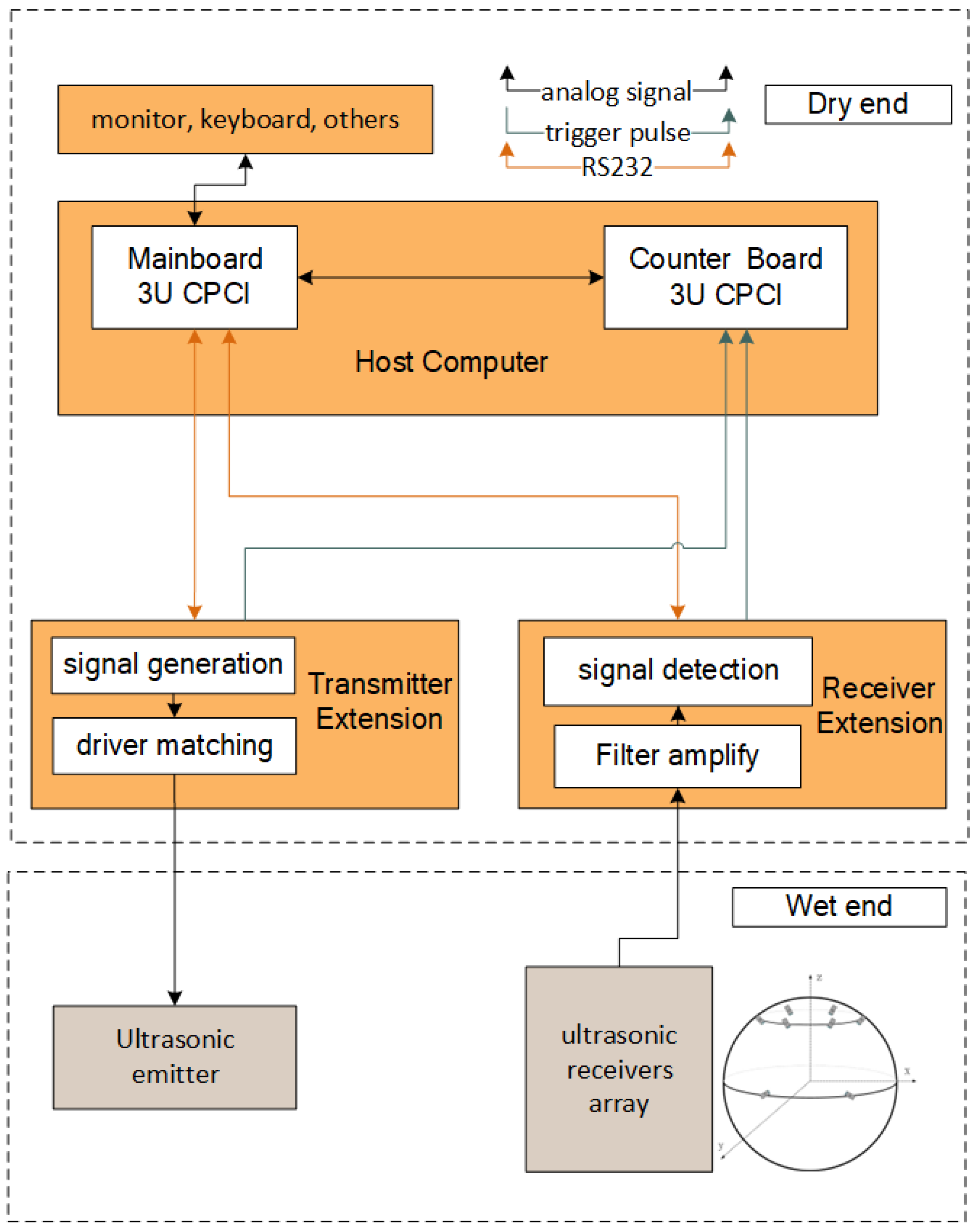
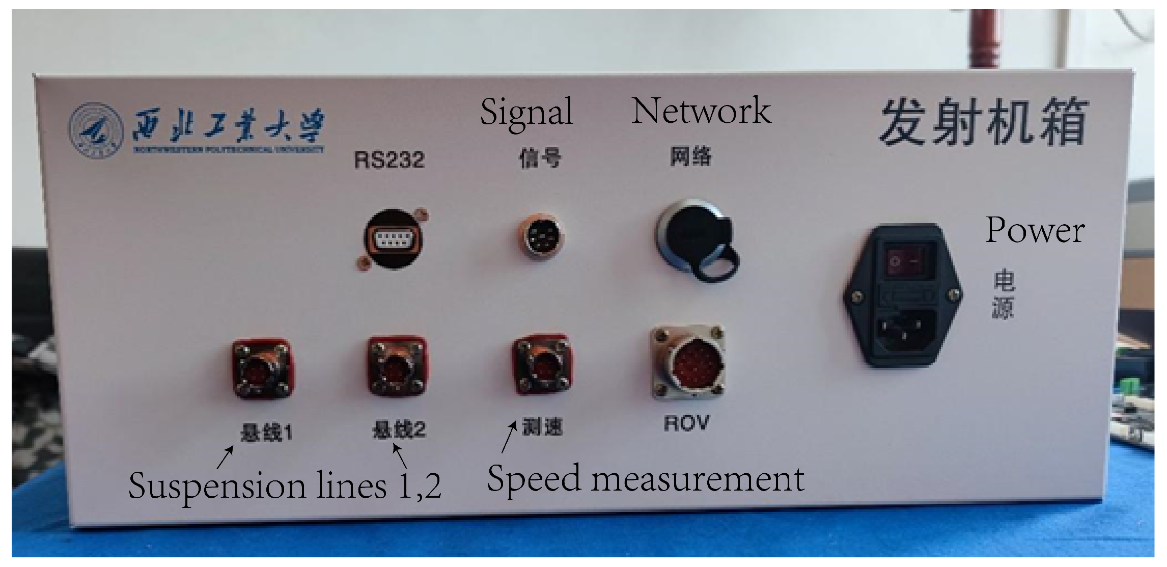
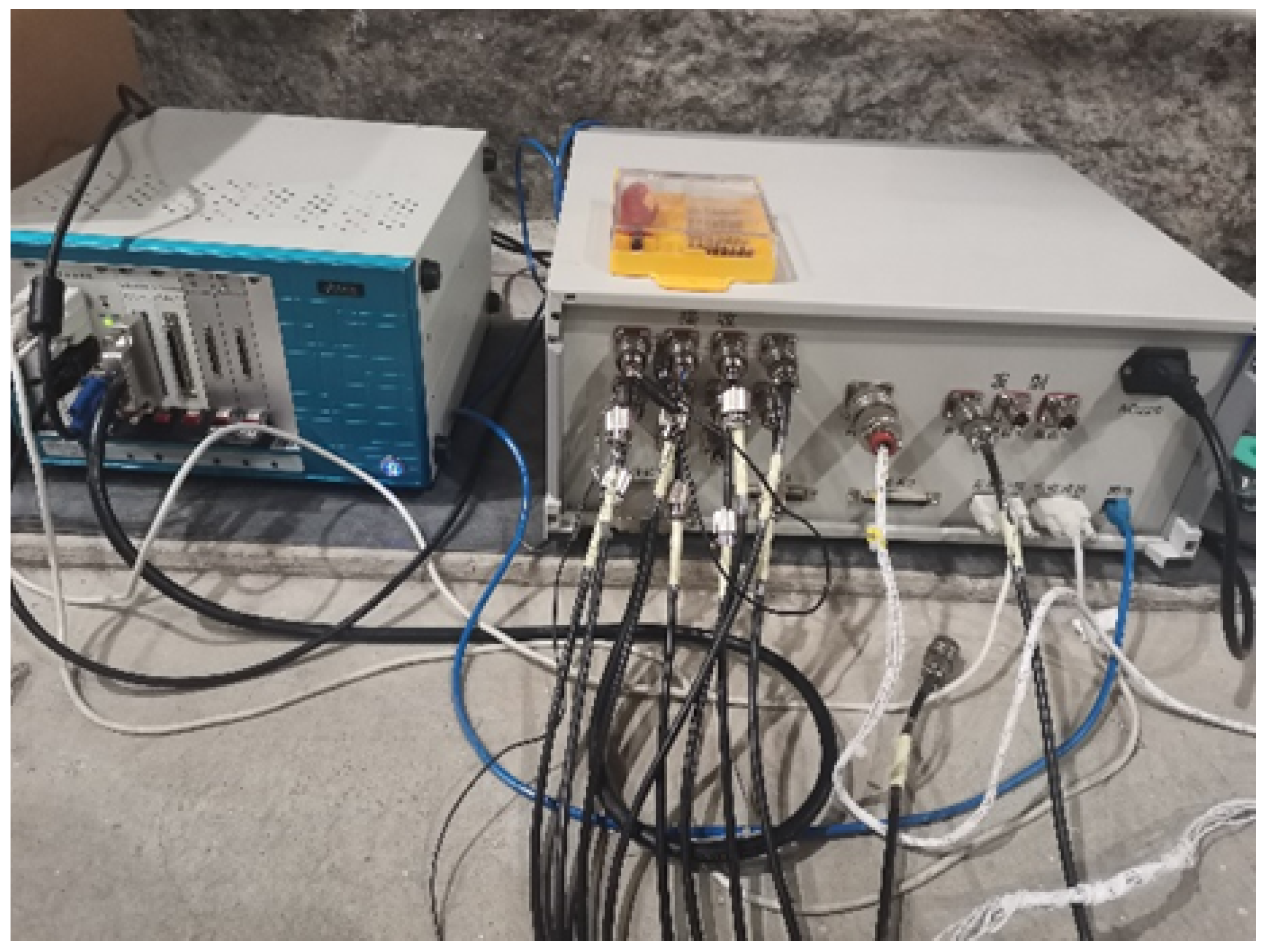
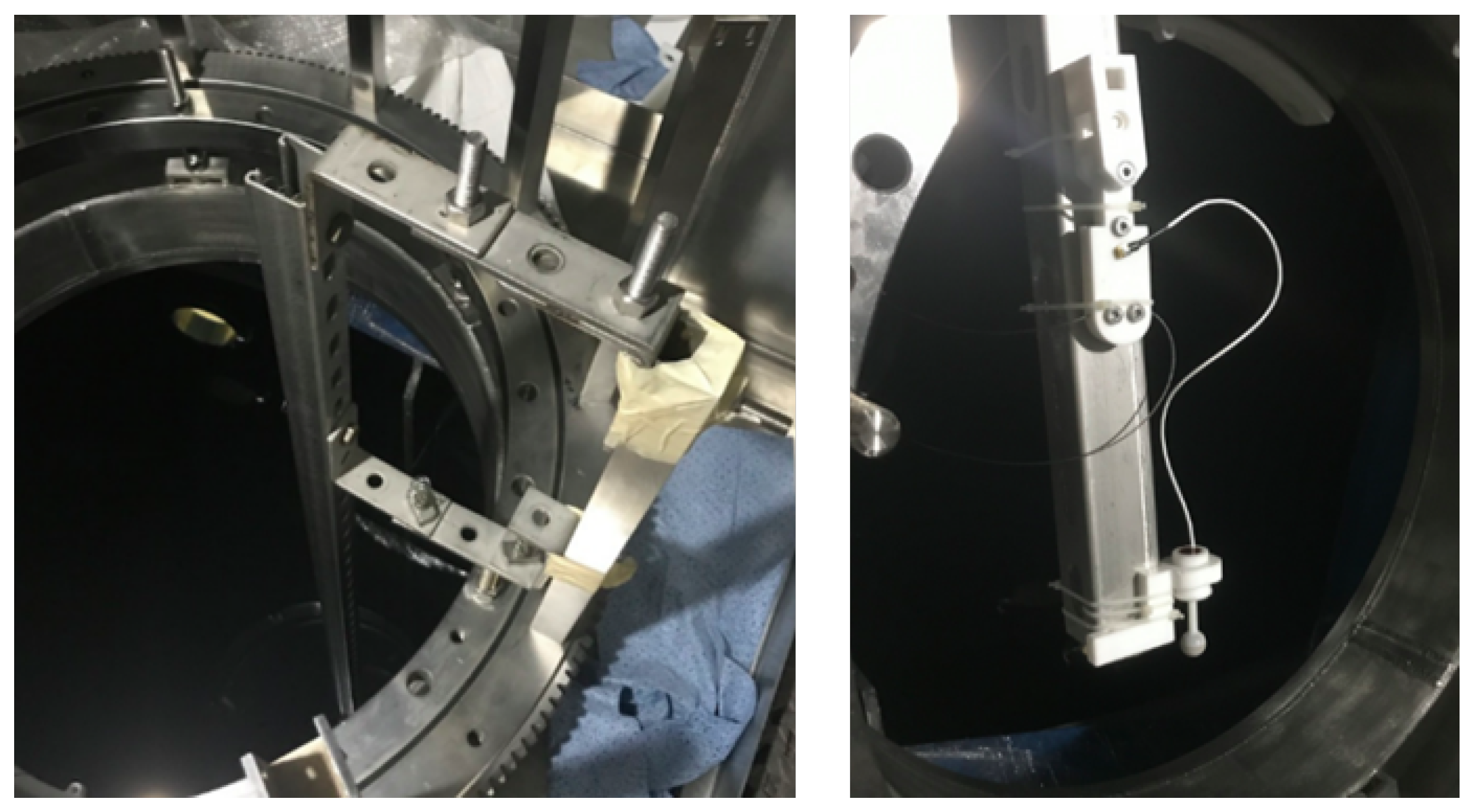
2. Configuration of Ultrasonic Positioning System

The block diagram of a complete system, including the host computer, transmitter extension, receiver extension, ultrasonic emitter, and an array of ultrasonic receivers is depicted in Figure 1. The host computer, transmitter extension, and receiver extension are the dry end equipment of the system, and the ultrasonic emitter and the array of ultrasonic receivers are the wet end equipment of the system, which will be placed into alkyl benzene in the CD when the system is working [17,18,19].

The host computer is the center of data processing and command, which controls the working of the transmitter extension and receiver extension, processes the inputs and outputs of interaction information, and carried out coordinate positioning of the ultrasonic emitter [20,21]. The control of the transmitter extension parameters is performed via the serial port, including the transmission channel, transmission pulse width, transmission cycle, transmission power, etc. [22]. In the same way, the control of the receiver extension parameters is completed through the serial port, including the selection of the receiving mode and channel, the receiving gain, etc. [23]. The host computer calculates the time delay between the starting trigger pulse of the transmitter extension and the ending trigger pulse of the receiver extension by the counter board card, obtains multiple groups of distance information, and then performs the real-time calculation and display of the coordinates of the ultrasonic emitter [24,25,26].

The transmitter extension is shown in Figure 2. According to the command of the host computer, the transmitter extension generates the required transmission signal, selects the transmission channel, and matches the ultrasonic emitter [27]. The frequency, pulse width, period, and amplitude of the transmission signal shall meet the corresponding requirements and send the start trigger pulse signal to the host computer [28].

The receiver extension is shown in Figure 3. According to the command of the host computer, the receiver extension can select the receiving mode, the receiving channel, and the filter; amplify, detect, and identify the signals received by the array of ultrasonic receivers; and send the end trigger pulse signal to the host computer [29,30].

The ultrasonic emitter is shown in Figure 4. It converts electrical signals into acoustic signals of a specific frequency and waveform set by the host computer. The ultrasonic emitter meets the compatibility with alkyl benzene, and its weight is less than 200 g to reduce the load weight. The ultrasonic emitter realizes omnidirectional transmission close to 4 $\pi$ to ensure that multiple ultrasonic receivers of the array can receive the transmission signal.

The ultrasonic receiver is shown in Figure 5. It converts acoustic signals into electrical signals for subsequent signal detection and processing. The beam width of the half power point of the ultrasonic receiver must be greater than 120°, and the ultrasonic receiver must meet the radiation safety requirements because it will work in the CD for a very long time.

3. Realization of Ultrasonic Positioning

The basic working principle of the ultrasonic positioning system is to obtain the distance information by computing the propagation time delay of the sound signal in alkyl benzene and then obtain the position of the ultrasonic emitter through the geometric relationship formed by the multi-point distance information. The ultrasonic receivers of the array are arranged in the CD (coordinates are known). When the position of the ultrasonic emitter needs to be determined, the host computer controls the transmitter extension to transmit ultrasonic signals through the ultrasonic emitter, according to the set parameters. The acoustic signals are transmitted to the ultrasonic receivers, where the receiver extension feeds back the arrival times (end trigger pulses) to the host computer after signal pre-processing and detection. The host computer calculates the distance between the ultrasonic emitter and each different ultrasonic receiver of the array by the time differences between the arrival times of the sound signal (end trigger pulses) and the start time of the sound signal (start trigger pulse). The current position of the ultrasonic emitter is computed, exploiting the multiple sets of distance and the coordinates of each ultrasonic receiver. Next, the implementation of the ultrasonic positioning will be introduced.

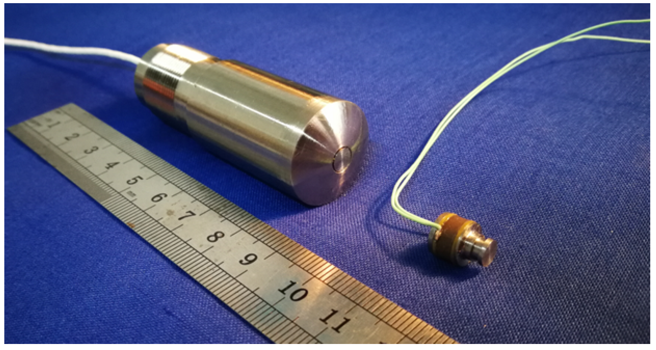
3.1. Design of Ultrasonic Receivers Array

In order to meet the radiation requirements of the CD and considering the requirements of positioning capability, the receiving array consists of eight ultrasonic receivers. Among them, No. 1 to No. 6 ultrasonic receivers are located in a circle at a latitude of 30 deg in the upper part of the CD sphere, evenly spaced by 60 deg. The No. 1 and No. 7 ultrasonic receivers are on the same longitude, as well as the No. 2 and No. 8 ultrasonic receivers. The No. 7 and No. 8 ultrasonic receivers are located at the equatorial plane. The array of ultrasonic receivers is shown in Figure 6.

The horizontal aperture of the ultrasonic receivers’ array is about 17.5 m, and the vertical aperture is about 15.2 m, meeting the aperture requirements for three-dimensional coordinate positioning.

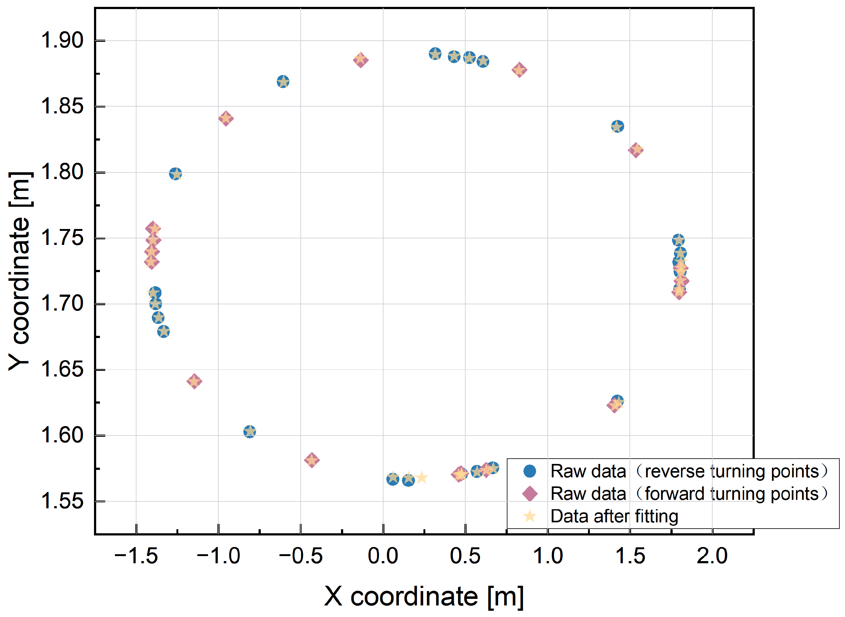
3.2. Positioning Algorithm

The positioning algorithm is based on time of arrival (TOA). The algorithm uses three or more ultrasonic receivers to locate the position of the ultrasonic emitter by exploiting the distance information from the ultrasonic emitter to the ultrasonic receivers. The three-dimensional coordinates of the ultrasonic emitter are therefore obtained. Considering M ultrasonic receivers, let the coordinate of the ith ultrasonic receiver be $(x_i,y_i,z_i)$ and the coordinate of the ultrasonic emitter be $(x,y,z)$; then, the three-dimensional spherical equations can be written as

$$\left\{\begin{array}{c}\sqrt{{\left(x-x_1\right)}^2+{\left(y-y_1\right)}^2+{\left(z-z_1\right)}^2}=s_1=c·{\tau }_1\\ \sqrt{{\left(x-x_2\right)}^2+{\left(y-y_2\right)}^2+{\left(z-z_2\right)}^2}=s_2=c·{\tau }_2\\ ⋮\\ \sqrt{{\left(x-x_M\right)}^2+{\left(y-y_M\right)}^2+{\left(z-z_M\right)}^2}=s_M=c·{\tau }_M\end{array}\right.$$

(1)

where $s_i$ is the distance between the ultrasonic emitter and the ith ultrasonic receiver, ${\tau }_i$ is the time of flight between ultrasonic emitter, and the ith ultrasonic receiver and $\widehat{c}$ is the speed of sound in transmission medium. For Equation (1), the conventional solution is to square each group of equations on both sides of the equation and eliminate the quadratic term to obtain the linear equations of the $M-1$ element.

$$\left\{\begin{array}{c}\left(x_2-x_1\right)x+\left(y_2-y_1\right)y+\left(z_2-z_1\right)z={\displaystyle \frac{s_1^2-s_2^2+r_1^2-r_2^2}{2}}\\ \left(x_3-x_2\right)x+\left(y_3-y_2\right)y+\left(z_3-z_2\right)z={\displaystyle \frac{s_2^2-s_3^2+r_2^2-r_3^2}{2}}\\ ⋮\\ \left(x_M-x_{M-1}\right)x+\left(y_M-y_{M-1}\right)y+\left(z_M-z_{M-1}\right)z={\displaystyle \frac{{s_{M-1}}^2-s_M^2+r_{M-1}^2-r_M^2}{2}}\end{array}\right.$$

(2)

where $r_i=\sqrt{x_i^2+y_i^2+z_i^2}$ is the 2-norm of the three-dimensional coordinate vector of the ith ultrasonic receiver. The matrix A and vector C can be defined as follows, so that Equation (2) can be written as a matrix equation in the form $AX=C$.

$$\mathbf{A}=\left[\begin{array}{ccc}{x}_2-x_1& y_2-y_1& z_2-z_1\\ x_3-x_2& y_3-y_2& z_3-z_2\\ ⋮& \\ x_M-x_{M-1}& y_M-y_{M-1}& z_M-z_{M-1}\end{array}\right],\mathbf{C}=\left[\begin{array}{c}{s}_1^2-s_2^2+r_1^2-r_2^2/2\\ s_2^2-s_3^2+r_2^2-r_3^2/2\\ ⋮\\ s_{M-1}^2-s_M^2+r_{M-1}^2-r_M^2/2\end{array}\right]$$

(3)

When $det\left(\mathbf{A}\right)\ne 0$, the unique solution of the coordinates of the ultrasonic emitter can be solved, as follows:

$$\mathbf{X}=\left[xyz\right]={\mathbf{A}}^{-1}\mathbf{C}$$

(4)

For matrix ${\mathbf{A}}_{(M-1)\times 3}$, if the number of ultrasonic receivers M is more than 4, then $\mathbf{A}$ cannot take the inverse operation. The positioning problem described in Equation (1) is also a curve fitting problem in the type of an optimization problem. The objective function consisting of the sum of squares of several functions can be written as follows:

$$F\left(\mathbf{X}\right)=\sum _{i=1}^M{f}_{\overline{i}}^2\left(\mathbf{X}\right)$$

(5)

Solving $X={[x,y,z]}^T$ for function $F\left(\mathbf{X}\right)$ solves the positioning result; then, it turns into a minimization problem, as follows:

$$minF\left(\mathbf{X}\right)=\sum _{i=1}^{M-1}{f}_i^2\left(\mathbf{X}\right)$$

(6)

Each $f_i\left(\mathbf{X}\right)$ is a function of $\mathbf{X}$; Equation (5) is also called the least squares problem. The principle of the least squares positioning algorithm is similar to Equation (2). By subtracting the unknowns of the equation group in Equation (5) one by one, the linear function of $\mathbf{X}$ is obtained.

$$f_i\left(\mathbf{X}\right)=p_i\mathbf{X}-c_i,i=1,2\dots ,M-1$$

(7)

where $p_i=\left[\begin{array}{ccc}{x}_{i+1}-x_i\hfill & y_{i+1}-y_i\hfill & z_{i+1}-z_i\hfill \end{array}\right]$, $c_i={\widehat{s}}_i^2-{\widehat{s}}_{i+1}^2+r_i^2-r_{i+1}^2/2$. The equations of the least squares location problem are rewritten as

$$\begin{array}{cc}\hfill F\left(\mathbf{X}\right)& =\sum _{i=1}^{M-1}{f}_i^2\left(\mathbf{X}\right)=\left[f_1\left(\mathbf{X}\right),f_2\left(\mathbf{X}\right),\dots ,,f_{M-1}\left(\mathbf{X}\right)\right]\left[\begin{array}{c}{f}_1\left(\mathbf{X}\right)\\ f_2\left(\mathbf{X}\right)\\ ⋮\\ f_{M-1}\left(\mathbf{X}\right)\end{array}\right]\hfill \\ \hfill & ={(\mathbf{A}\mathbf{X}-\mathbf{C})}^T(\mathbf{A}\mathbf{X}-\mathbf{C})={\mathbf{X}}^T{\mathbf{A}}^T\mathbf{A}\mathbf{X}-2{\mathbf{C}}^T\mathbf{A}\mathbf{X}+{\mathbf{C}}^T\mathbf{C}\hfill \end{array}$$

(8)

where matrices $\mathbf{A}$ and $\mathbf{C}$ are same as that of Equation (3). To solve $minF\left(\mathbf{X}\right)$ is same as solving the minimum point of convex function $F\left(\mathbf{X}\right)$, that is, we need to solve the equation as shown below. If the column of $\mathbf{A}$ is a full-rank column and ${\mathbf{A}}^T\mathbf{A}$ is a positive-definite matrix, the extreme value of the objective function is the solution result of the unknown $\mathbf{X}$:

$$\mathbf{X}={\left({\mathbf{A}}^T\mathbf{A}\right)}^{-1}{\mathbf{A}}^T\mathbf{C}$$

(9)

4. Test and Discussion

In order to verify the effectiveness of the ultrasonic localization system, a functional performance verification experiment of the localization system was carried out at the Neutrino Experiment Station (NES) within the Daya Bay Nuclear Power Station. The experimental setup was located in a cylindrical stainless steel tank vessel with a diameter of 5 m and a height of 5 m. The experimental setup was run in the same environment as JUNO’s experimental setup. Except for the different container size, the environment configuration in Daya Bay is basically the same as that of JUNO’s experiment, with the interior of the cylindrical container filled with an alkyl benzene solution of 98% purity. Since the volume of the stainless steel canister is much smaller than that of the CD in JUNO’s experimental site, the temperature difference of the alkyl benzene solution inside the canister is negligible, and the speed of sound in the environment was measured with a miniature speed of sound profiler (mini-svp) as 1382.571 m/s through real-time testing. The coordinates of eight ultrasonic receivers placed in a stainless steel tank are accurately determined by optical calibration using a total station, and the array is laid out as shown in Figure 7, with the origin of the coordinates located at the center of the bottom of the tank. Figure 8 shows a detail of the test setup. The depth coordinate information is provided by the high-precision pressure sensor that is included with the ultrasonic emitter. The sensor in question is capable of achieving an accuracy of approximately millimeters, which is significantly more precise than the accuracy achievable with the setup. Consequently, the present study will limit its verification of the effect of positioning to the horizontal XY coordinate plane.

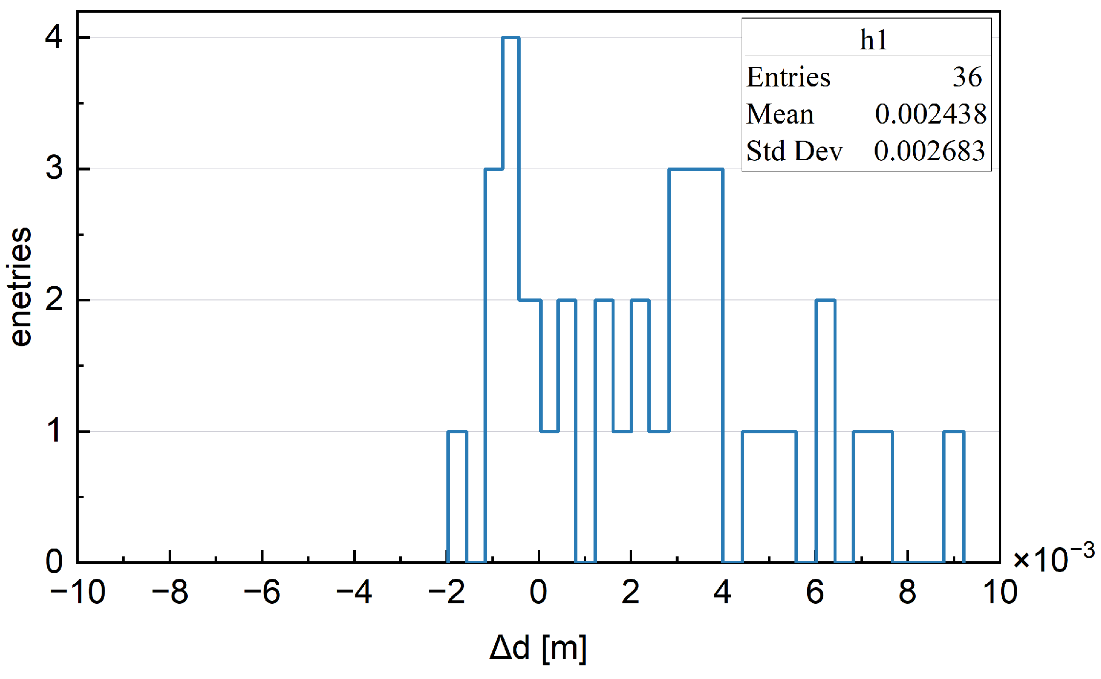
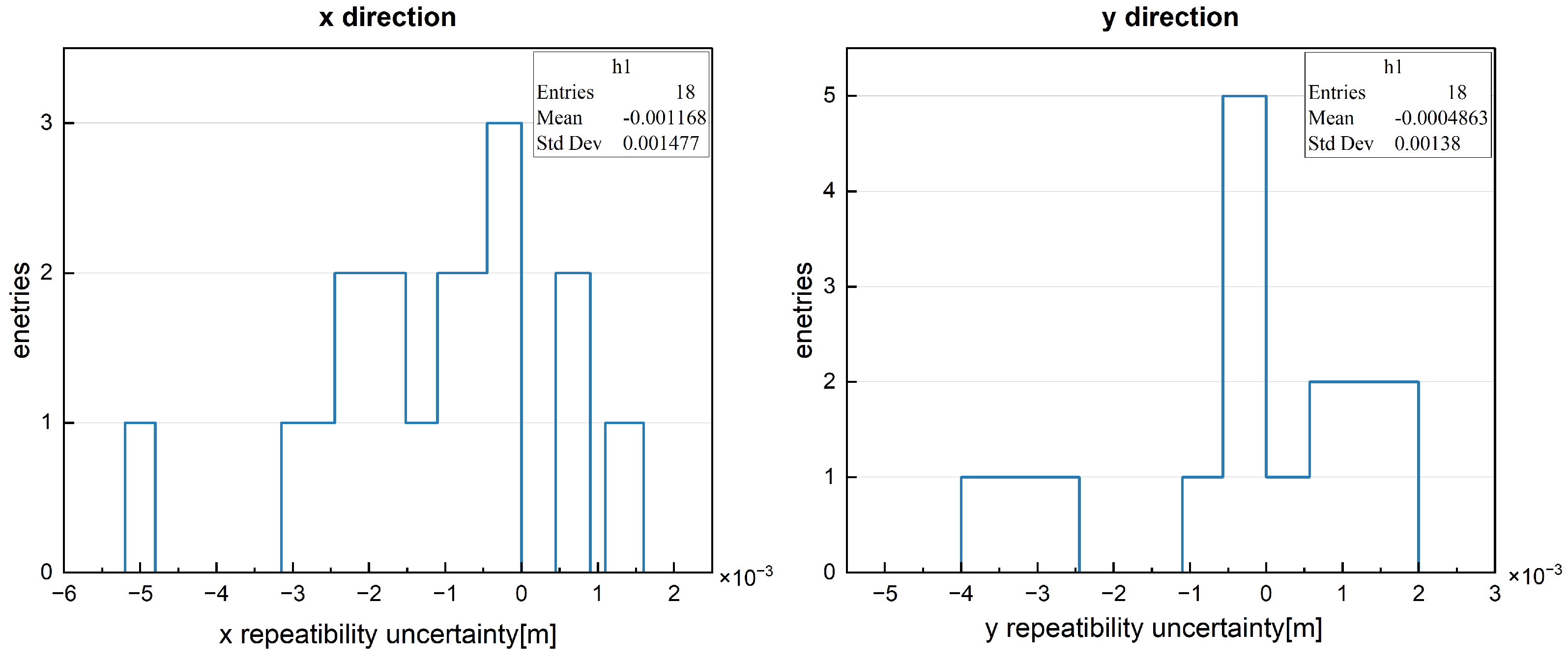
4.1. Positioning Consistency Experiment

First, the verification of measurement consistency is made through horizontal linear motion. In a 4.2 m high horizontal plane, the transmitting transducer is vertically moved downward, and it moves back and forth 0.5 m horizontally and in a straight line through the push rod. The experimental device is shown in Figure 9. The push rod moves in steps of 1 cm or 5 cm each time. Moving by 19 points in the positive direction (forward), the corresponding Y coordinate differences of adjacent points are computed and shown by the pink lines in Figure 10. Moving backward by 18 points in the negative direction and returning to the original position, the corresponding differences of Y coordinates of adjacent points are computed and shown by the blue lines in Figure 10. The X coordinate difference of 36 adjacent points is reported in Figure 11, showing that the values are less than 4 mm. The UPS (Ultrasonic Positioning System) is used to measure the plane position coordinates of each point three times, and then the average values are taken. The maximum difference between the measured displacement and the expected displacement of 36 points is less than 1 cm, as shown in Figure 12. The positioning coordinate error of 18 repeated points in forward and reverse motions is less than 0.6 cm in the X direction and less than 0.5cm in the Y direction, as shown in Figure 13.

The depth of the ultrasonic emitter is then changed to a new position, at a 3.9 m high horizontal plan, and the positioning experiment is repeated for 36 points. Each point is measured three times, and the average is taken. The maximum difference between the measured displacement and the expected displacement is still less than 1 cm. The results are shown in Figure 14, indicating that different depths have no effect on the positioning results.

4.2. Positioning Accuracy Experiment

The ultrasonic emitter makes circular motion by the connecting rod driven by the source library, as shown in Figure 15. The source library is an external gear that can be precisely rotated to a specified angle with a servo motor drive system. Some of the rotation angles of the source library are small steps (3°) and some are large steps (30°). First, one clockwise rotation is performed, passing through 25 points, as shown by the pink square in Figure 16; then, one counterclockwise rotation is performed, passing through 16 points, as shown by the blue circle in Figure 16.

By fitting the position coordinates of these 41 measured points, we can reconstruct the motion trajectory of the transmitting transducer. The fitting curve is shown by the green line in Figure 16. The trajectory presents a basically standard circular shape, which is consistent with the circular motion of the actual transmitting transducer, indicating that the trend is correct.

The corresponding fitted points evaluated from the fitting curve are shown by the orange star in Figure 17. The fitted points are compared with the actual point positions to perform the positioning error analysis. The positioning errors are shown in Figure 18, where the positioning errors of the 25 forward turning points shown in pink, and the positioning errors of the 16 reverse turning points are shown in blue. The maximum positioning error is less than 2.5 mm, indicating that the system has good positioning accuracy.

5. Conclusions

In this paper, considering that JUNO’s experimental setup was filled with a liquid scintillator (alkyl benzene), we reported the performance of an ultrasonic localization system implemented through an array of eight receivers and one emitter, and we tested it in an experimental setup in Daya Bay. We showed that the ultrasonic localization system can effectively locate the target position. A comparison of the localization results with the real coordinates of the target, through consistency and accuracy experimental verifications, respectively, showed that the localization results had good reliability. In order to meet the size requirements of the JUNO in practice, this study demonstrated through simulations and experiments that the horizontal six-element array aperture of the JUNO can meet the 3 cm accuracy requirement as long as it exceeds 12 m [31].

In the selection of the positioning method, considering the limitation of the number of arrays and the reliability of the positioning results, the TOA-based positioning method was selected and combined with the range information of the eight-element transducer array for the simulation study. In the future, the TOA method can be combined with the received signal strength (RSS) method to further improve the localization accuracy in JUNO scenarios.

References

1. An, F.; An, G.; An, Q.; Antonelli, V.; Baussan, E.; Beacom, J.; Bezrukov, L.; Blyth, S.; Brugnera, R.; Avanzini, M.B.; et al. Neutrino physics with JUNO. J. Phys. Nucl. Part. Phys. 2016, 43, 030401. [Google Scholar] [CrossRef]
2. Ye, X.C.; Yu, B.X.; Zhou, X.; Zhao, L.; Ding, Y.Y.; Liu, M.C.; Ding, X.F.; Zhang, X.; Jie, Q.L.; Zhou, L.; et al. Preliminary study of light yield dependence on LAB liquid scintillator composition. Chin. Phys. C 2015, 39, 096003. [Google Scholar] [CrossRef]
3. He, M.; JUNO Collaboration. Jiangmen underground neutrino observatory. Nucl. Part. Phys. Proc. 2015, 265, 111–113. [Google Scholar] [CrossRef]
4. Wang, Z. JUNO central detector and its prototyping. J. Phys. Conf. Ser. 2016, 718, 062075. [Google Scholar] [CrossRef]
5. Wang, J.; Anfimov, N.; Guo, J.Y.; Gu, Y.; Hu, H.; Li, M.; Ma, Q.M.; Olshevskiy, A.; Peng, Z.Y.; Qin, Z.H.; et al. Database system for managing 20,000 20-inch PMTs at JUNO. Nucl. Sci. Tech. 2022, 33, 24. [Google Scholar] [CrossRef]
6. Zhu, G.L.; Liu, J.L.; Wang, Q.; Xiao, M.J.; Zhang, T. Ultrasonic positioning system for the calibration of central detector. Nucl. Sci. Tech. 2019, 30, 5. [Google Scholar] [CrossRef]
7. Zhang, R.; Cao, D.W.; Loh, C.W.; Liu, Y.H.; Wu, F.L.; Zhang, J.L.; Qi, M. Using monochromatic light to measure attenuation length of liquid scintillator solvent LAB. Nucl. Sci. Tech. 2019, 30, 30. [Google Scholar] [CrossRef]
8. Zhang, Y.; Liu, J.; Xiao, M.; Zhang, F.; Zhang, T. Laser calibration system in JUNO. J. Instrum. 2019, 14, P01009. [Google Scholar] [CrossRef]
9. Zhang, Y.; Hui, J.; Liu, J.; Xiao, M.; Zhang, T.; Zhang, F.; Meng, Y.; Xu, D.; Ye, Z. Cable loop calibration system for Jiangmen underground neutrino observatory. Nucl. Instrum. Methods Phys. Res. Sect. A Accel. Spectrometers Detect. Assoc. Equip. 2021, 988, 164867. [Google Scholar] [CrossRef]
10. Feng, K.; Li, D.; Shi, Y.; Qin, K.; Luo, K. A novel remotely operated vehicle as the calibration system in JUNO. J. Instrum. 2018, 13, T12001. [Google Scholar] [CrossRef]
11. Teng, D.; Liu, J.L.; Zhu, G.L.; Meng, Y.; Zhang, Y.y.; Zhang, T.; Luo, K.; Li, R.; Hui, J.Q. Low-radioactivity ultrasonic hydrophone used in positioning system for Jiangmen Underground Neutrino Observatory. Nucl. Sci. Tech. 2022, 33, 76. [Google Scholar] [CrossRef]
12. Patel, M.; Chitaliya, N.; Shukla, Y. Design and implementation of underwater positioning system using GPS surface node and acoustic signals. Int. J. Adv. Res. Eng. Sci. Technol. 2017, 4, 35–41. [Google Scholar]
13. Zhang, J.; Han, Y.; Zheng, C.; Sun, D. Underwater target localization using long baseline positioning system. Appl. Acoust. 2016, 111, 129–134. [Google Scholar] [CrossRef]
14. Tallini, I.; Iezzi, L.; Gjanci, P.; Petrioli, C.; Basagni, S. Localizing autonomous underwater vehicles: Experimental evaluation of a long baseline method. In Proceedings of the IEEE 2021 17th International Conference on Distributed Computing in Sensor Systems (DCOSS), Pafos, Cyprus, 14–16 July 2021; pp. 443–450. [Google Scholar]
15. Tang, Z. Long baseline underwater acoustic location technology. In Encyclopedia of Ocean Engineering; Springer: Singapore, 2022; pp. 935–941. [Google Scholar]
16. Cario, G.; Casavola, A.; Gagliardi, G.; Lupia, M.; Severino, U. Accurate localization in acoustic underwater localization systems. Sensors 2021, 21, 762. [Google Scholar] [CrossRef] [PubMed]
17. Cui, P.; Jiang, K.; Lv, J.; Zhao, Z.; Yue, J.; Jiao, D. A Hydroacoustic Positioning Method Based on Analysis of the Error Region of Three-circle Intersection. In Proceedings of the IEEE 2021 OES China Ocean Acoustics (COA), Harbin, China, 14–17 July 2021; pp. 763–766. [Google Scholar]
18. Chugunov, A.; Kulikov, R.; Pudlovskiy, V. Modeling a High-Precision Positioning Algorithm for Acoustic Positioning System. In Proceedings of the IEEE 2020 International Multi-Conference on Industrial Engineering and Modern Technologies (FarEastCon), Vladivostok, Russia, 6–9 October 2020; pp. 1–5. [Google Scholar]
19. Ahmed, A.; Hamid, U.; Masud, A.; Waqas, M.; Ali, S. Simulation of ultra short baseline system for positioning of underwater vehicles. In Proceedings of the IEEE 2022 19th International Bhurban Conference on Applied Sciences and Technology (IBCAST), Islamabad, Pakistan, 16–20 August 2022; pp. 944–950. [Google Scholar]
20. Saeid, L. Underwater Source Localization based on Modal Propagation and Acoustic Signal Processing. Master’s Thesis, University of Windsor, Windsor, ON, Canada, 2021. [Google Scholar]
21. Yang, T.; Zhao, J. Solution to long-range continuous and precise positioning in deep ocean for autonomous underwater vehicles using acoustic range estimation and inertial sensor measurements. J. Shanghai Jiaotong Univ. (Sci.) 2022, 27, 281–297. [Google Scholar] [CrossRef]
22. Graça, P.A.A. Relative Acoustic Localization with USBL (Ultra-Short Baseline). Master’s Thesis, Faculty of Engineering—University of Porto, Porto, Portugal, 2020. [Google Scholar]
23. Guo, H.; Li, L.; Zhang, S. Short baseline direct position determination based on precise synchronization. In Proceedings of the IET International Radar Conference (IET IRC 2020), Chongqing, China, 4–6 November 2020. [Google Scholar]
24. Yoshihara, T.; Ebihara, T.; Mizutani, K.; Sato, Y. Underwater acoustic positioning in multipath environment using time-of-flight signal group and database matching. Jpn. J. Appl. Phys. 2022, 61, SG1075. [Google Scholar] [CrossRef]
25. Yoshihara, T.; Ebihara, T.; Mizutani, K.; Sato, Y. Underwater Acoustic Positioning Using Time-of-flight Signal Blocks. In Proceedings of the Symposium on Ultrasonic Electronics, Online, 11–16 September 2021; Volume 42, pp. 2E3–E4. [Google Scholar]
26. Zhang, Q.; Guo, Y.; Heng, Y.; Zhou, L.; Yu, B.; Liu, J.; Xiao, M.; Zhang, F. JUNO central detector and its calibration system. In Proceedings of the 38th International Conference on High Energy Physics, Venice, Italy, 5–12 July 2017; SISSA Medialab: Trieste, Italy, 2017; Volume 282, p. 967. [Google Scholar]
27. Zhu, G.; Wang, Q.; Cheng, Q. Accurate ultrasonic positioning system for the Central Detector. In Proceedings of the IEEE OCEANS 2019, Marseille, France, 17–20 June 2019; pp. 1–4. [Google Scholar]
28. Hladky-Hennion, A.C.; Dubus, B. Finite element analysis of piezoelectric transducers. In Piezoelectric and Acoustic Materials for Transducer Applications; Springer: New York, NY, USA, 2008; pp. 241–258. [Google Scholar]
29. Zhang, Y.; Wang, L.; Qin, L.; Zhong, C.; Hao, S. Spherical–omnidirectional piezoelectric composite transducer for high-frequency underwater acoustics. IEEE Trans. Ultrason. Ferroelectr. Freq. Control 2020, 68, 1791–1796. [Google Scholar] [CrossRef] [PubMed]
30. Teng, D.; Yang, H.; Zhu, G. Design and test about high sensitivity thin shell piezoelectric hollow sphere hydrophone. In Proceedings of the IEEE OCEANS 2017, Anchorage, AK, USA, 18–21 September 2017; pp. 1–6. [Google Scholar]
31. Zhu, G.; Wang, Y.; Wang, Q. Research on Accurate Ultrasonic Positioning Error under the Special Environment. Xibei Gongye Daxue Xuebao/J. Northwestern Polytech. Univ. 2018, 36, 496–501. [Google Scholar] [CrossRef]
Figure 1. Block diagram of ultrasonic positioning system.
Symmetry 16 01218 g001
Figure 2. Transmitter extension.
Symmetry 16 01218 g002
Figure 3. Receiver extension.
Symmetry 16 01218 g003
Figure 4. Ultrasonic emitter.
Symmetry 16 01218 g004
Figure 5. Ultrasonic receiver.
Symmetry 16 01218 g005
Figure 6. Schematics of the ultrasonic receiver array positioning in the CD.
Symmetry 16 01218 g006
Figure 7. Schematic diagram of the ultrasonic receivers’ array test setup based on JUNO’s experimental scenarios.
Symmetry 16 01218 g007
Figure 8. Picture of a detail showing three ultrasonic receivers of the ultrasonic receivers’ array based on’s experimental scenarios.
Symmetry 16 01218 g008
Figure 9. Horizontal motion measuring: (left) Launcher and lifting structure. (center) Kevlar rope suspension, leveling. (right) Actuators precisely change displacement.
Symmetry 16 01218 g009
Figure 10. Y coordinate difference between adjacent points scenarios.
Symmetry 16 01218 g010
Figure 11. X coordinate difference between adjacent points scenarios.
Symmetry 16 01218 g011
Figure 12. Difference between measured and expected (4.2 m) scenarios.
Symmetry 16 01218 g012
Figure 13. Coordinate error of the same position scenarios.
Symmetry 16 01218 g013
Figure 14. Difference between measured and expected (3.9 m) scenarios.
Symmetry 16 01218 g014
Figure 15. Circular motion measuring: (left) Source library-driven circular motion. (right) Ultrasonic emitter fixation.
Symmetry 16 01218 g015
Figure 16. Plot of raw points and fitting curves.
Symmetry 16 01218 g016
Figure 17. Distribution of original and fitting points.
Symmetry 16 01218 g017
Figure 18. Positioning error for forward and reverse motion.
Symmetry 16 01218 g018
Disclaimer/Publisher’s Note: The statements, opinions and data contained in all publications are solely those of the individual author(s) and contributor(s) and not of MDPI and/or the editor(s). MDPI and/or the editor(s) disclaim responsibility for any injury to people or property resulting from any ideas, methods, instructions or products referred to in the content.