A Study on Network Anomaly Detection Using Fast Persistent Contrastive Divergence

Abstract

As network technology evolves, cyberattacks are not only increasing in frequency but also becoming more sophisticated. To proactively detect and prevent these cyberattacks, researchers are developing intrusion detection systems (IDSs) leveraging machine learning and deep learning techniques. However, a significant challenge with these advanced models is the increased training time as model complexity grows, and the symmetry between performance and training time must be taken into account. To address this issue, this study proposes a fast-persistent-contrastive-divergence-based deep belief network (FPCD-DBN) that offers both high accuracy and rapid training times. This model combines the efficiency of contrastive divergence with the powerful feature extraction capabilities of deep belief networks. While traditional deep belief networks use a contrastive divergence (CD) algorithm, the FPCD algorithm improves the performance of the model by passing the results of each detection layer to the next layer. In addition, the mix of parameter updates using fast weights and continuous chains makes the model fast and accurate. The performance of the proposed FPCD-DBN model was evaluated on several benchmark datasets, including NSL-KDD, UNSW-NB15, and CIC-IDS-2017. As a result, the proposed method proved to be a viable solution as the model performed well with an accuracy of 89.4% and an F1 score of 89.7%. By achieving superior performance across multiple datasets, the approach shows great potential for enhancing network security and providing a robust defense against evolving cyber threats.

1. Introduction

The advancement of the internet and network technology has brought us many conveniences, but it has also led to a surge in various forms of cyberattacks. Attackers are trying to exploit related vulnerabilities to steal information or break into secure networks [1]. These attacks can be carried out in a variety of ways, including privacy breaches, data tampering, and denial-of-service attacks, so it is important to have a network security system in place. Among cyber attacks, D-Dos attacks are responsible for up to 25% of all internet traffic in a country [2]. It is essential to analyze the traffic generated to understand the path of the attacked network to prepare for the next attack or to gather information to defend against an ongoing attack.

Intrusion detection systems are a critical component of network security that analyze network traffic to detect malicious activity or policy violations in real time [3]. Intrusion detection methods are categorized into three main categories [4]. They can be categorized into signature-based detection, anomaly-based detection, and stateful protocol analysis. Signature-based detection is a method of detecting anomalies using signatures that represent patterns or strings of characters that correspond to known attacks or threats. It is the process of analyzing and comparing captured events and patterns to detect intrusions, using knowledge accumulated by specific attacks and system vulnerabilities. Anomaly-based detection detects behavior that does not correspond to known behavior and uses profiles that represent normal and expected behavior derived from monitoring regular activity, network connections, hosts, or users over a period of time. These can be static or dynamic and can be developed for a variety of attributes, such as failed login attempts, processor usage, number of emails sent, etc. Next, the observed events are compared to the normal profile to recognize significant attacks. This is also known as behavior-based detection. Some examples of anomalous behavior-based detection include intrusion attempts, penetration of legitimate users, denial of service, and Trojans. Finally, stateful protocol analysis indicates that an IDS can identify and track the protocol state. Although it looks similar to anomaly detection, it is also called specification-based detection because it relies on generic profiles developed by vendors for specific protocols. Typically, SPA’s network protocol models are based on protocol standards originally developed by international standards organizations (e.g., IETF). They differ in that they focus on specific attacks/threats or unknown attacks. Among IDS methodologies, anomaly detection methods can detect zero-day attacks because they detect anomalous behavior by modeling normal behavior. However, modeling normal behavior is a very difficult problem, so anomaly detection techniques using machine learning and deep learning techniques have been actively researched recently [5]. Machine learning and deep learning are suitable because they can model data and predict and infer outcomes, but most of the data suffer from imbalance, as the data in the minority class are much smaller than the data in the majority class [6]. In general, classification performance is likely to suffer when using AI models, and the detection of minority classes becomes difficult as the model is trained to be biased toward one side.

Recent studies have used support vector machines (SVMs) and autoencoders (AEs) for training to solve this data imbalance problem and anomaly detection problem. However, AEs have the disadvantage of over-reconstructing some samples, which degrades the performance of the detection method, and SVMs have difficulty understanding the inherent structure of the data and extracting features from noisy or incomplete data. The symmetry between performance and training time must be considered. In this paper, DBNs are used, which learn complex representations of data, extract robust features from incomplete data through unsupervised and semi-supervised learning, and learn multi-level representations. DBN is a structure of multiple layers of restricted Boltzmann machines, where each layer can learn the complex hierarchical structure of the data [7,8]. The weights of each layer can be efficiently initialized to alleviate the gradient vanishing problem, which enables structured and hierarchical dictionary learning compared to AE.

Recent research has focused on high accuracy, and as the structure of the model becomes increasingly complex, the learning speed of the model becomes slower. To address this, this paper uses a fast-continuous-contrast-divergence–deep-belief-network-based model to effectively deal with uncertainty and ambiguity in the data. High-dimensional data features are then extracted through the deep neural network structure, and precise detection is performed based on them.

The organization of this paper is as follows: Section 2 describes the network intrusion detection approach, which uses deep learning models to detect anomalies. Section 3 describes the DBN model using the fast continuous contrast divergence method proposed in this paper. In Section 4, anomalies are detected using the NSL-KDD, UNSW-NB15, and CIC-IDS-2017 datasets to conduct experiments and compare the performance with that of other studies. Conclusions are drawn, and future work is presented in Section 5.

2. Related Works

Intrusion detection aims to identify and alert you to security threats such as unauthorized access, malicious activity, or policy violations [9]. It primarily works based on predefined intrusion signatures, which are derived from known attack types. Identifying malicious traffic with a specific pattern, such as DDoS attacks, is an example of intrusion detection. Time series anomaly detection aims to detect unusual patterns, fluctuations, or anomalies in time series data [10]. It is used in a variety of fields to analyze changes in data over time. It is used by leveraging machine learning or deep learning techniques to analyze the statistical characteristics or behavioral patterns of data. Both methodologies process and analyze large amounts of data to detect anomalies. They also monitor data flows and raise alerts when anomalies are detected. This requires fast analytics on continuous data streams. In terms of detecting anomalies in large and complex network data, intrusion detection and time series anomaly detection techniques can be used in combination to improve the effectiveness of security systems and help detect and respond to more diverse and sophisticated attacks and threats.

2.1. Deep-Learning-Based Network Intrusion Detection

Yang et al. [11] proposed a model that combines an improved conditional variational autoencoder (ICVAE) and a deep neural network (DNN). New attack samples were generated according to the specified intrusion categories to balance the training data and increase the diversity of training samples to improve the detection rate of unbalanced attacks. Since the class labels are only used as additional input to the decoder, the learned weights can be reused. By automatically reducing the data dimensionality and reusing ICVAE to initialize the weights of the DNN’s hidden layers, global optimization can be easily achieved through backpropagation and fine-tuning.

Radford et al. [12] tokenize netflows and compress them into word sequences that form sentences representing conversations between computers and then create a model that learns the semantic and syntactic grammar of the generated language. It uses long short-term memory (LSTM) and recurrent neural networks (RNNs) to capture the complex relationships and nuances of language. It predicts the communication between two IPs and uses the error to measure how typical or pessimistic the observed communication is. By training a model that is unique to each network but generalized to typical traffic, both internal and external, sequences of network activity that are outliers can be identified. Positive unsupervised attack identification performance was demonstrated on an ISCX IDS dataset containing normal traffic and four attack patterns.

Kim et al. [13] developed a deep-learning-based CNN model focusing on Dos attacks. They used the KDD99 dataset and classified the attacks into two categories, attack and benign, focusing on different attacks that fall into the same category rather than broad categories. In addition to KDD 99, they also used CIC IDS 2018 to use a sufficient sample of data and compared its performance with RNNs, showing good performance.

Tian et al. [14] proposed a method called ramp-OCSVM by introducing a ramp loss function to develop a robust and sparse methodology to address the shortcomings of traditional noise-sensitive SVMs. By utilizing the advantages of its non-convexity property, a robust and sparse semi-supervised algorithm was created. The concave–convex procedure (CCCP) was utilized to solve the obtained model, which is an infeasible non-convex optimization problem. The performance was measured using the NSL-KDD and UNSW-NB15 datasets, and the superiority of the model in terms of parameter sensitivity analysis and sparsity was demonstrated.

Zavrak et al. [15] used a variational autoencoder (VAE) with a focus on detecting anomalous network traffic rather than flow-based data. They used flow features to identify unknown attacks and flow-based features extracted from network traffic data, including common and different types of attacks. To analyze the performance of the method at different thresholds, the Receiver Operating Characteristic (ROC) curves were examined in detail, and it was found that the method outperforms other models.

Kim et al. [16] used LSTM networks to model system call sequences and interpret program execution into the system call language. They used a robust ensemble method that combines multiple models to reduce the high false alarm rate and demonstrated an improved ability to identify both known and unknown attacks. Their method is efficient in detecting host-based anomalies and demonstrates improved precision in detecting intrusions by focusing on short sequences of system calls.

Aldwairi et al. [17] recognized the ability to recognize new attack patterns due to the high dimensionality of network traffic data as one of the key requirements for anomaly detection systems. Restricted Boltzmann machine (RBM) was used to distinguish between normal and abnormal traffic in the ISCX dataset. The effectiveness of the RBM was tested using real-world positive and negative measurements along with its accuracy, and the bias that appears during training was reduced by eliminating data imbalance and using a balanced dataset.

Sharma et al. [18] proposed a feed-forward deep neural network (FFDNN) method based on deep learning methodology using a filter-based feature selection model. The feature selection strategy aims to determine and select the most relevant subset of attributes from the feature importance scores for training a deep learning model. They implemented a method to remove unnecessary and inefficient features from the feature importance scores and experimented with NSL-KDD, UNSW-NB15, and CIC-IDS-2017 datasets, showing good performance. While this provides good generalization power, there is a risk that not enough features of the data exist or that important information is missing as parameter values change.

Sharma et al. [19] used a concatenative learning model based on different convolutional neural network (CNN) models, VGG16, VGGG19, and Xception, and experimented with the UNSW-NB15 and CIC-DDOS-2019 datasets. During pre-training, the images were converted into square color images suitable for CNN model application using feature selection techniques based on information gain values. However, while combining multiple neural network layers improves performance, it also increases the size and complexity of the model, which increases training time and computational cost. Because they are based on DNN models, additional tuning is essential to adapt to new types of attacks or changing data patterns.

While the above-mentioned studies have contributed a lot, there are a few problems. Some of the studies were conducted on only one dataset instead of multiple datasets, and since attackers rarely leave traces in real-world network environments, their practical application is limited. To solve this problem, this research conducts experiments on various datasets and conducts anomaly detection research on normal datasets, excluding anomalous data to measure suspicious data from trace-free network traffic records.

2.2. Deep Belief Network

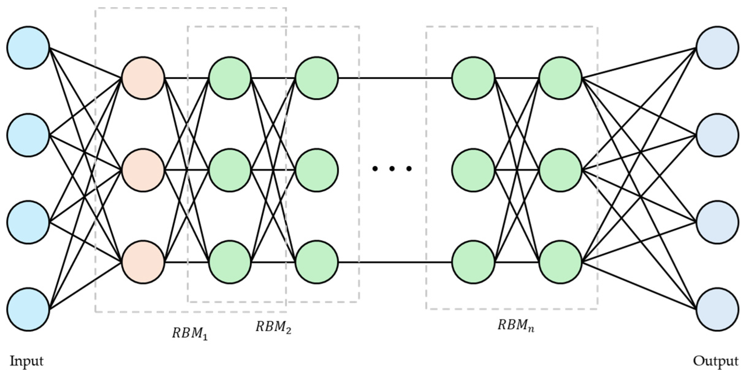
A deep belief network (DBN) is one of the generative probabilistic graphical models, which consists of several layers of unsupervised learning models, most notably RBMs. Each layer trains independently, and the training results of the lower layers are used as input data for the higher layers. The DBN structure can be seen in Figure 1, where the RBMs in each layer use an energy function to determine the probability distribution of the system.

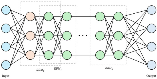
Figure 1. Structure of deep belief network.

The energy function can be represented as in Equation (1), where $v$ is the state of the neurons in the visible layer, $b$ and $c$ are the biases of the visible and hidden neurons, respectively, and $w_{ij}$ is the weight between neurons $i$ and $j$.

$$E\left(v,h\right)=-\left(\sum _i{b}_i{v}_i+\sum _j{c}_j{h}_j+\sum _{i,j}{v}_i{w}_{ij}{h}_j\right)$$

(1)

This can be expressed as the combined probability of a neuron and a hidden neuron as shown in Equation (2). $Z$ is the partition function; normalize the probability distribution so that the sum of the probabilities is 1.

$$P\left(v,h\right)={\displaystyle \frac{e^{-E\left(v,h\right)}}{Z}}$$

(2)

The conditional probabilities of the visible and hidden neurons can be calculated as shown in Equations (3) and (4); let $\sigma \left(x\right)$ be a sigmoid function, where $\sigma \left(x\right)=1/(1+e^{-x})$.

$$P\left(h_j=1|v\right)=\sigma \left(c_j+\sum _i{w}_{ij}{v}_i\right)$$

(3)

$$P\left(v_j=1|h\right)=\sigma \left(b_i+\sum _j{w}_{ij}{h}_j\right)$$

(4)

2.3. Contrastive Divergence

The contrastive divergence (CD) algorithm, commonly used in machine learning, updates the weights as shown in Equation (5) [20].

$$w_{ij}^{(t+1)}=w_{ij}^{\left(t\right)}+\eta \left({⟨v_i{h}_j⟩}_{data}-{⟨v_i{h}_j⟩}_{model}\right)$$

(5)

The data expectation (${⟨v_i{h}_j⟩}_{data}$) represents the product of the average visible units $v_i$ and hidden units $h_j$ computed from the model’s response to the input data and represents the average activation state based on the actual data distribution. The model expectation value (${⟨v_i{h}_j⟩}_{model}$) is calculated based on the data reconstructed by the model and represents the average activation state from the data distribution generated by the model. In the $C{D}_n$ algorithm, n refers to the number of Gibbs sampling steps performed between the visible and hidden units, which has a significant impact on the learning rate or weights.

Persistent contrastive divergence (PCD) is a method that does not randomly initialize the initial state of a Markov chain, but instead continuously maintains the state of the chain from the previous training step and uses it as the starting point for the next training [21]. It helps the chain better converge to the data distribution and generate idealized, theoretically accurate samples. Continuous chaining reduces the mismatch between the model distribution and the data distribution and provides stable and balanced learning. However, it has the disadvantage of slow convergence compared to the CD algorithm, which makes learning take longer.

To solve this problem, a method that uses fast weights is applied. Fast weights and fast learning rates are used to fine-tune the energy surface and are related to stochastic gradient ascent or gradient-based optimization methods [22].

$$h^{+}=P\left(h|v^{+}, \theta -regular\right)$$

(6)

$$g^{+}=v^{{+}^T}{h}^{+}$$

(7)

In the positive phase, we calculate the probability of the hidden layer $h^{+}$ as shown in Equation (6). We then calculate the positive gradient between the actual data $v^{+}$ and the activation of the hidden layer $h^{+}$ by the extrinsic, as shown in Equation (7). $\theta -regular$ is used to compute the probability of the hiding layer $h^{+}$ for $v^{+}$ and to find the positive gradient $g^{+}$.

$$h^{-}=P\left(h|v^{-}, \theta -regular+\theta -fast \right)$$

(8)

$$g^{-}=v^{{-}^T}{h}^{-}$$

(9)

In Equation (8), the sum of $\theta -regular$ and $\theta -fast$ is used to calculate the probability of the hiding layer $h^{-}$ for $v^{-}$. Here, $\theta -fast$ helps the model adapt to the rapidly changing nature of the data. In Equation (9), ${v^{-}}^T$ and $v^{-}$ are used to find the negative gradient $g^{-}$. Then, $\theta -fast$ is used to perform a Gibbs sampling step to update the Markov chain and compute the full gradient $g$. $\theta -fast$ is then adjusted by updating the value of $\theta -regular$ and applying a fast learning rate. The difference maximized by the parameter can measure the deviation of the model distribution from the distribution from which the fantasy particles were sampled, and this parameter update alternates with the Gibbs update of the chain. This ensures that the slope has a positive cosine value for a discrete probability distribution but prevents it from becoming too large. The weight updates increase this slope, but the persistent chains quickly mix, which quickly decreases the slope, resulting in the two products canceling out.

3. Fast-Persistent-Contrastive-Divergence-Method-Based Deep Belief Network

3.1. Dataset Preprocessing

To detect anomalies using artificial intelligence models, a network intrusion detection dataset needs to be available. Open datasets for model training contain symbolic data that cannot be used as input. They contain values that are missing, too small, too large, or diverge into infinity. To address this, the dataset needs to be transformed into a form that is easier for the model to learn from, a process known as data preprocessing.

To improve the quality of the data so that the model can learn effectively, data cleaning fixes or removes incomplete or inaccurate data. Missing values can be removed from the data, imputed using statistical methods, or estimated using a predictive model. If a predictive model is used, all instances of data containing missing values should be removed before training, as this could cast doubt on the reliability of the results. Simple incremental counters, attributes that contain meaningless information, and fields with constant values are also removed to reduce training time and increase efficiency.

Sometimes, a piece of data has multiple attribute values, and those attributes are in different formats. Information like time can be changed to a simple real value like unix timestamp, or text information like a network address can be converted to a real or integer value. This is known as data transformation and embedding, which is the process of transforming data that is difficult to represent into a form that is easier to capture its characteristics through embedding. Since data values are often spread over a wide range, it is necessary to unify the units and ranges. This is called data normalization, and it is essential to embed non-numerical values by scaling them to a certain range of values.

To account for the nature of each attribute and preserve as many existing values as possible, we used min–max scaling for numeric data (including both integers and real numbers). Min–max scaling is a method of scaling an attribute to a specific range. In this study, we used a scale between 0 and 1 to train the model. This research used a logarithmic transformation because large variations in values, such as the number of bytes in a packet, load data, or rate, can cause normal data to be misclassified as outliers. Logarithmic transformation is an effective way to reduce the scale of the data and reduce the impact of large values or outliers. This transformation can significantly reduce the scale of the values, reducing their skewing of the overall data distribution. For data represented as strings, such as protocol, state, attack category, and label, we used encoding to convert them to integers. One of the methods considered was one-hot encoding, but due to the large number of categories in the data, the dimensionality of the data increased rapidly, so we used a simple method, label encoding, to sequentially number and convert them.

Learning all the features is a very bad choice for efficiency. Instead, it is essential to select and learn the key features that contain the unique information in the data. Traditional dimensionality reduction techniques, such as principal component analysis (PCA), can reduce dimensionality by summarizing the main variability into a few principal components. However, it has limitations in capturing the characteristics of data with non-linear structure, such as network data, and is sensitive to noise because it is based on the covariance of all variables.

In this study, we use the FPCD algorithm for dynamic evaluation of attribute importance. It allows us to evaluate the degree of activation of each trait in the hidden layer, select only those traits that really contribute to the model, and remove less important traits. DBNs are multi-layered, with each layer reconstructing the data and producing more abstract and information-dense attributes as one moves to higher layers. Although there are other methods of entropy-based attribute selection and correlation analysis between attributes, we use the attribute importance method because it does not involve complex preprocessing by analyzing each weight value in the model and does not change the overall structure of the neural network model, allowing for efficient processing. The attribute importance can be represented using the contribution of each attribute, which can be expressed as in Equation (10). The activation probability is calculated as in Equation (3). The activation probability is calculated from Equation (3), which quantitatively evaluates the influence of each input characteristic in hidden layer learning.

$$Attribution\left(i\right)=\sum _j\left|w_{ij}\right|\times P(h_j=1|v)$$

(10)

3.2. Training FPCD-DBN

The probability of a data point is calculated from the distribution of the joint probability of the states of the hidden layer neurons h for a given state v of the visible neurons in the RBM. It is calculated using an energy function, such as Equation (2) described in Section 2.2, and represents how well a particular data point is explained. To simplify the training data points, data likelihood, or the log-likelihood of the data points, is used. It indicates how well the model describes the dataset, and is calculated as follows:

$$logP\left(v\right)=log\sum _h{e}^{-E(v,h)}-log Z$$

(11)

It plays an important role in optimizing the parameters of the model and uses a positive gradient of the log-likelihood over the data points. It guides the model’s parameter updates based on the actual data distribution. It represents the gradient of the log-likelihood calculated from the samples generated by the model and based on the model distribution. This difference is used to update the model parameters. Equations (12) and (13) describe how the regular parameter θ-regular and the fast parameter θ-fast are updated, respectively. These equations represent the process of updating the parameters using the difference between the positive gradient $g^{+}$ and the negative gradient $g^{-}$, which is used as a metric to measure how well the model reproduces the training data. The regular parameters provide the stability and generalization ability of the model, while the fast parameters help the model adapt quickly to changes in the data. Using a harmonized update of the two variables allows the model to learn the data more accurately and quickly. And we can see that the learning rate adjusts over time in Equation (14). It starts with a high learning rate at the beginning and gradually tapers off, with the model quickly finding approximate parameter values early in training and fine-tuning over time to achieve a more precise optimization.

$${\theta }_{regular}⟵{\theta }_{regular}+{\eta }_{regular}·(g^{+}-g^{-})$$

(12)

$${\theta }_{fast}⟵{\theta }_{fast}+{\eta }_{fast}·(g^{+}-g^{-})$$

(13)

$${\eta }_{regular}\left(t\right)={\eta }_{inital}\times \left(1-{\displaystyle \frac{t}{T_{max}}}\right)$$

(14)

4. Experiments

Several experiments were conducted to validate the FPCD-DBN model in a network intrusion detection environment. Experiments were performed on three different datasets and compared with results from other studies. Instead of multi-class detection, a binary classification problem was pursued to classify normal and attack instances. Since the boundary between the two classes can be clearly defined and optimized, the characteristics of the classes can be better understood, and accurate predictions can be made. And because it uses data from both classes, it can effectively handle data imbalance. It is believed that binary classification is more suitable than single-class classification because the performance of the model does not need to be reduced as long as clear labels are present in the public dataset, which has already been proven reliable by many studies. The DBN configuration used in the experiments is shown in Table 1.

Table 1. The DBN configuration.

Parameter	Value
Hidden Layer Dimension	12-6-3
Batch Size	64
Momentum	0.9
Activation Function	ReLU, Sigmoid
Optimizer/Learning Rate	Adam/0.001
Loss Function	MSE

4.1. Datasets

Among publicly available datasets for network intrusion detection, the NSL-KDD dataset, the UNSW-NB15 dataset, and the CIC-IDS-2017 dataset are used in this paper. The NSL-KDD dataset was developed to address issues with the widely used KDD Cup 99 dataset. While the KDD Cup 99 dataset was useful for training models to detect specific types of attacks, it tended to have poor generalization performance due to a large number of duplicate records and unrealistically different test and training sets. The NSL-KDD dataset reduces the risk of overfitting by removing duplicate data and ensuring data diversity. It also better reflects real-world network environments, making the model’s performance evaluation more reliable. The dataset includes different types of attack scenarios, allowing us to evaluate the ability of network security systems to detect different intrusions. It includes four types of attacks, with categories such as denial of service (Dos), user-2-root (U2R), remote local-to-local (R2L), and probing attack (Probe). However, since the dataset is outdated, the UNSW-NB15 dataset was used as an additional dataset. The UNSW-NB15 dataset contains more network traffic characteristics, ranging from low-level network packet data to high-level characteristics, which allows for more complex analysis and algorithm development [23]. It better reflects network technologies and environments, such as IoT environments and cloud services, and includes detailed descriptions and metadata to help simulate specific situations. Furthermore, the training and test data were effectively separated, ensuring reliable performance evaluation. The main types of attacks covered by the UNSW-NB15 dataset are categorized as fuzzers, analysis, backdoors, DoS, exploits, generic, reconnaissance, shellcode, worms, and normal. CIC-IDS-2017 includes a variety of the latest attack scenarios and provides more realistic traffic patterns and attack scenarios based on traffic generated by real networks [24]. It has the advantage of providing detailed labels for each network event and more than 80 network traffic features, which is superior in both the quality and quantity of data. It includes attack types such as Heartbleed, web attack, infiltration, botnet, DDos, ftp-patator, ssh-patator, etc.

The NSL-KDD and UNSW-NB15 datasets were used as they were distributed as separate training and testing datasets. For the CIC-IDS-2017 dataset, since the types of attacks vary by day of the week, the provided data were combined, and 200,000 samples were randomly selected for training. Table 2 shows the number of benigns and attacks in the training and test datasets for each dataset.

Table 2. The number of normal and attacks in the dataset used in the experiment.

Title 1	Train Dataset		Test Dataset
	Benign	Attack	Benign	Attack
NSL-KDD	67,343	58,630	12,833	9711
UNSW-NB15	119,341	56,000	45,332	37,000
CIC-IDS-2017	1,704,822	418,234	568,275	139,412

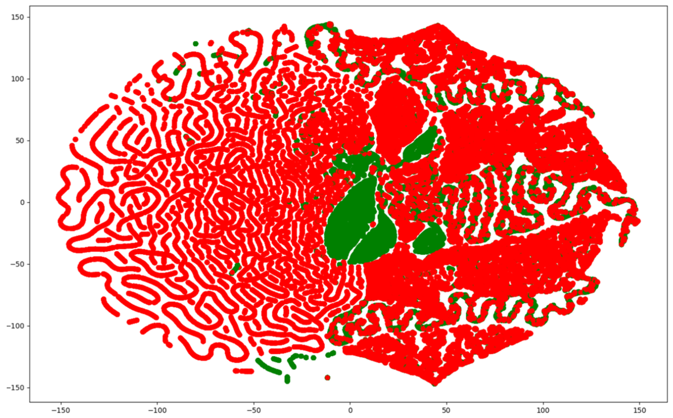
Since network traffic data are represented as high-dimensional vectors, they can be visualized using various methods. Among them, the t-distributed Stochastic Neighbor Embedded (t-SNE) method is capable of embedding in low dimensions while preserving the binary structure between data represented by high-dimensional vectors. Figure 2, Figure 3 and Figure 4 visualize the NSL-KDD, UNSW-NB15, and CIC-IDS-2017 datasets using the t-SNE technique. They show that the benign and attack samples share the same feature space in some places, making anomaly detection difficult and linear separation impossible.

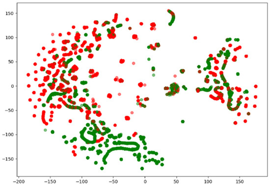
Figure 2. Visualization of the NSL-KDD dataset using t-SNE.

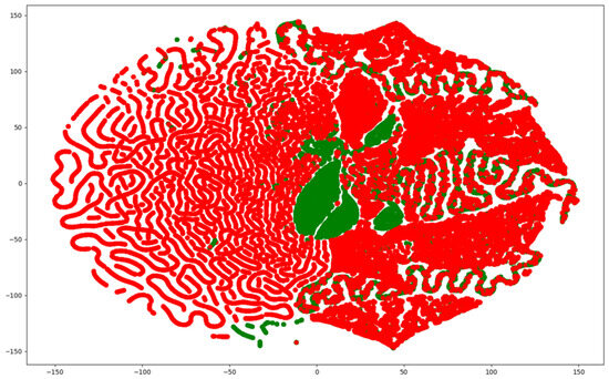
Figure 3. Visualization of the UNSW-NB15 dataset using t-SNE.

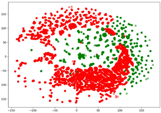
Figure 4. Visualization of the CIC-IDS-2017 dataset using t-SNE.

4.2. Performance Evaluation

Performance is measured using the confusion matrix, a metric often utilized in the literature to evaluate the performance of models, as shown in Table 3. Accuracy describes the percentage of times a model correctly predicts the total predictions, but it is not as reliable when there is a class imbalance, as high accuracy can be achieved by predicting a large number of classes if samples from one class dominate. Precision is measured to determine how accurate a prediction is and is considered an important metric when the goal is to minimize the number of false positives. Recall, also called sensitivity, is an important metric to ensure that true positive cases are not missed. $F1-Score$ represents the harmonic mean of Precision and Recall and is useful when considering both metrics simultaneously. It allows for the evaluation of how well-balanced the model is and is characterized by a sharp drop in score if either aspect is low.

$$Accuracy={\displaystyle \frac{TP+TN}{TP+TN+FP+FN}}$$

(15)

$$Precision={\displaystyle \frac{TP}{TP+FP}}$$

(16)

$$Recall={\displaystyle \frac{TP}{TP+FN}}$$

(17)

$$F1-score=2\times {\displaystyle \frac{Precision\times Recall}{Precision+Recall}}$$

(18)

Table 3. Confusion matrix.

		Predicted
		Positive	Negative
Actual	Positive	True Positive (TP)	False Negative (FN)
	Negative	False Positive (FP)	True Negative (TN)

4.3. Experimental Results

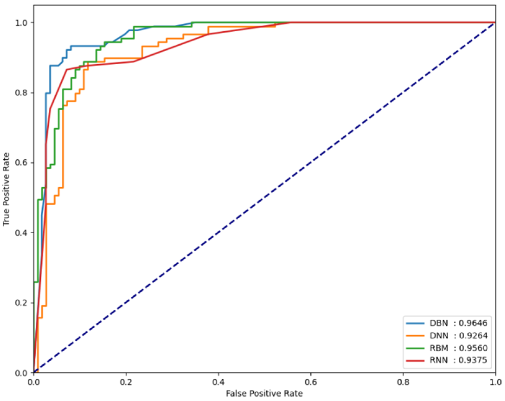
For the classification performance results of each model to be meaningful in the experiments, it is necessary to verify whether each model is sensitive to changes in the threshold value. To verify this, the FPCD-DBN, RBM, DNN, and RNN models proposed in this paper, along with the area under receiver operating characteristic (AU-ROC), were used. By analyzing the performance metrics on each dataset, the extent of the changes in model performance can be observed. Basically, the closer the ROC curve is to the upper left, the better the model, which indicates that the normal and attack error distributions are very far apart. It also means that the performance is not sensitive to small changes in the determined threshold, which means that this threshold can be used as a good decision boundary in testing. Figure 5, Figure 6 and Figure 7 show the AUROC of the models for each dataset.

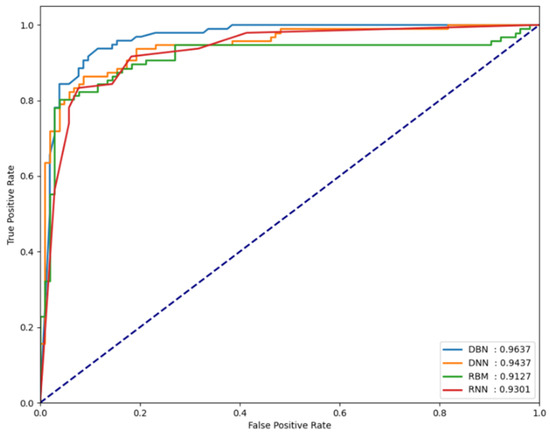
Figure 5. AUROC values measured for the NSL-KDD dataset.

Figure 6. AUROC values measured for the UNSW-NB15 dataset.

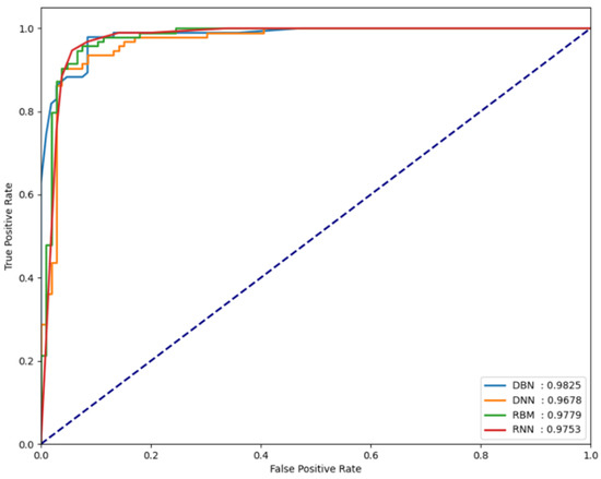
Figure 7. AUROC values measured for the CIC-IDS-2017 dataset.

In our experiments, the AUROC performance for each dataset is shown in Table 4. In our experiments using the NSL-KDD dataset which following Table 5, the FPCD-DBN model showed an accuracy of 89.39% and an F1 score of 89.72%. This compares favorably to the 88.28% and 88.65% accuracies of similar autoencoders [25] in terms of identifying and reconstructing key features of the data. This can be explained by the fact that FPCD-DBN better captures the importance of the features in the data through continuous Markov chains, enabling high data adaptability. It also shows a high F1 score of 89.72% on the UNSW-NB15 dataset which following Table 6, compared to 83.2% and 85.26% for SSAE [26] and MemAE [27], respectively. This can be attributed to the predictive model’s ability to accurately identify the multi-layered structure and complex patterns in the data and learn the non-linear data characteristics more effectively, resulting in higher sensitivity and specificity.

Table 4. AUROC performance for each dataset.

Parameter	Value
	NSL-KDD	UNSW-NB15	CIC-IDS-2017
DBN	0.9637	0.9646	0.9825
DNN	0.9437	0.9262	0.9678
RBM	0.9127	0.9560	0.9779
RNN	0.9301	0.9375	0.9753

Table 5. Comparison of experimental results on the NSL-KDD dataset with other studies.

Methods	Metrics
	Accuracy	Precision	Recall	F1 Score
DNN [28]	0.7575	-	-	-
RNN-IDS [29]	0.8129	-	-	-
RT [30]	0.8621	0.8078	0.9416	0.8696
AE [25]	0.8828	0.9123	0.8786	0.8951
DAE [25]	0.8865	0.9648	0.8308	0.8928
LSTM [31]	0.8900	-	-	-
FPCD-DBN	0.8939	0.8951	0.8983	0.8972

Table 6. Comparison of experimental results on the UNSW-NB15 dataset with other studies.

Methods	Metrics
	Accuracy	Precision	Recall	F1 Score
NB [32]	0.7639	0.7820	0.7640	0.7729
SVM [33]	0.8190	0.9730	0.7560	0.8210
RF [26]	0.8363	0.8690	0.8360	0.8522
SSAE [26]	-	0.7310	0.9630	0.8320
MemAE [27]	0.8530	0.8774	0.8530	0.8526
FPCD-DBN	0.8662	0.8841	0.8816	0.8828

5. Conclusions

In this study, a deep belief network (DBN) was implemented using the fast persistent contrastive divergence (FPCD) technique to evaluate its performance on the NSL-KDD, UNSW-NB15, and CIC-IDS-2017 datasets. These datasets are significant in the area of network anomaly detection, and each reflects different levels of cybersecurity issues. During the experimental phase, the area under the receiver operating characteristic (AUROC) was used as the main measure to indirectly validate the performance of the model. This approach facilitated the identification of the appropriate threshold to be applied to each dataset, ensuring consistency in the evaluation.

The experimental results showed that the FPCD-enhanced DBN outperformed the existing models in terms of accuracy and F1 score. In particular, the model achieved impressive AUROC values. This suggests that the derived thresholds are not only appropriate for the various attack scenarios presented in the dataset but also effective as decision boundaries. When these results were compared to those of other studies, it was found that the model was able to handle imbalanced data, a common problem. The model demonstrates excellent classification results, achieving 89.4% on the NSL-KDD dataset and 86.6% on the UNSW-NB15 dataset. These results highlight not only the efficiency of the proposed model but also its robustness to detect a wide range of network anomalies under a variety of conditions. These findings confirm that the learning capabilities of the network can be greatly enhanced, making it highly effective for complex anomaly detection tasks in network security, considering the symmetry between performance and training time.

References

- Barbir, A.; Murphy, S.; Yang, Y. RFC 4593: Generic Threats to Routing Protocols. Available online: http://www.ietf.org/rfc/rfc4593.txt (accessed on 3 September 2024).
- Cisco Annual Internet Report (2018–2023) White Paper. Available online: https://www.cisco.com/c/en/us/solutions/collateral/executive-perspectives/annual-internet-report/white-paper-c11-741490.html (accessed on 3 September 2024).
- Bace, R.G.; Mell, P. Intrusion Detection Systems; Special Publication (NIST SP), Report Number 800-31; National Institute of Standards and Technology: Gaithersburg, MD, USA, 2001. Available online: https://www.nist.gov/publications/intrusion-detection-systems (accessed on 9 September 2024).
- Liao, H.J.; Lin, C.H.R.; Lin, Y.C.; Tung, K.Y. Intrusion detection system: A comprehensive review. J. Netw. Comput. Appl. 2013, 36, 16–24. [Google Scholar] [CrossRef]
- Pang, G.; Shen, C.; Cao, L.; Hengel, A.V.D. Deep learning for anomaly detection: A review. ACM Comput. Surv. (CSUR) 2021, 54, 1–38. [Google Scholar] [CrossRef]
- Hasib, K.M.; Iqbal, M.S.; Shah, F.M.; Mahmud, J.A.; Popel, M.H.; Showrov, M.I.H.; Ahmed, S.; Rahman, O. A survey of methods for managing the classification and solution of data imbalance problem. J. Comput. Sci. 2020, 16, 1546–1557. [Google Scholar] [CrossRef]
- Fischer, A.; Igel, C. An introduction to restricted Boltzmann machines. In Proceedings of the Progress in Pattern Recognition, Image Analysis, Computer Vision, and Applications: 17th Iberoamerican Congress, CIARP 2012, Buenos Aires, Argentina, 3–6 September 2012; pp. 14–36. [Google Scholar] [CrossRef]
- Hinton, G.E. Deep belief networks. Scholarpedia 2009, 4, 5947. [Google Scholar] [CrossRef]
- Xiao, C.; Gou, Z.; Tai, W.; Zhang, K.; Zhou, F. Imputation-based time-series anomaly detection with conditional weight-incremental diffusion models. In Proceedings of the 29th ACM SIGKDD Conference on Knowledge Discovery and Data Mining, Long Beach, CA, USA, 4 August 2023; pp. 2742–2751. [Google Scholar] [CrossRef]
- Xu, J.; Wu, H.; Wang, J.; Long, M. Anomaly transformer: Time series anomaly detection with association discrepancy. arXiv 2021, arXiv:2110.02642. [Google Scholar] [CrossRef]
- Yang, Y.; Zheng, K.; Wu, C.; Yang, Y. Improving the classification effectiveness of intrusion detection by using improved conditional variational autoencoder and deep neural network. Sensors 2019, 19, 2528. [Google Scholar] [CrossRef]
- Radford, B.J.; Apolonio, L.M.; Trias, A.J.; Simpson, J.A. Network traffic anomaly detection using recurrent neural networks. arXiv 2018, arXiv:1803.10769. [Google Scholar] [CrossRef]
- Kim, J.; Kim, J.; Kim, H.; Shim, M.; Choi, E. CNN-based network intrusion detection against denial-of-service attacks. Electronics 2020, 9, 916. [Google Scholar] [CrossRef]
- Tian, Y.; Mirzabagheri, M.; Bamakan, S.M.H.; Wang, H.; Qu, Q. Ramp loss one-class support vector machine; a robust and effective approach to anomaly detection problems. Neurocomputing 2018, 310, 223–235. [Google Scholar] [CrossRef]
- Zavarak, S.; Iskefiyeli, M. Anomaly-based intrusion detection from network flow features using variational autoencoder. IEEE Access 2020, 8, 108346–108358. [Google Scholar] [CrossRef]
- Kim, G.; Yi, H.; Lee, J.; Paek, Y.; Yoon, S. LSTM-based system-call language modeling and robust ensemble method for designing host-based intrusion detection systems. arXiv 2016, arXiv:1611.01726. [Google Scholar] [CrossRef]
- Aldwairi, T.; Perera, D.; Novotny, M.A. An evaluation of the performance of Restricted Boltzmann Machines as a model for anomaly network intrusion detection. Comput. Netw. 2018, 144, 111–119. [Google Scholar] [CrossRef]
- Sharma, H.S.; Singh, K.J. A feed forward deep neural network model using feature selection for cloud intrusion detection system. Concurr. Comput. Pract. Exp. 2024, 36, e8001. [Google Scholar] [CrossRef]
- Sharma, H.S.; Singh, K.J. Intrusion detection system: A deep neural network-based concatenated approach. J. Supercomput. 2024, 80, 13918–13948. [Google Scholar] [CrossRef]
- Carreira-Perpinan, M.A.; Hinton, G. On contrastive divergence learning. In Proceedings of the International Workshop on Artificial Intelligence and Statistics, Bridgetown, Barbados, 6–8 January 2005; Volume R5, pp. 33–40. Available online: https://proceedings.mlr.press/r5/carreira-perpinan05a.html (accessed on 3 September 2024).
- Berglund, M.; Raiko, T. Stochastic gradient estimate variance in contrastive divergence and persistent contrastive divergence. arXiv 2013, arXiv:1312.6002. [Google Scholar] [CrossRef]
- Tieleman, T.; Hinton, G. Using fast weights to improve persistent contrastive divergence. In Proceedings of the 26th Annual International Conference on Machine Learning Held in Conjunction with the 2007 International Conference on Inductive Logic Programming, Montreal, QC, Canada, 14–18 June 2009; pp. 1033–1040. [Google Scholar] [CrossRef]
- Moustafa, N.; Slay, J. NSW-NB15: A comprehensive data set for network intrusion detection systems (UNSW-NB15 network data set). In Proceedings of the 2015 Military Communications and Information Systems Conference (MilCIS), Canberra, ACT, Australia, 10–12 November 2015; pp. 1–6. [Google Scholar] [CrossRef]
- Stiawan, D.; Idris, M.Y.B.; Bamhdi, A.M.; Budiarto, R. CICIDS-2017 Dataset Feature Analysis With Information Gain for Anomaly Detection. IEEE Access 2020, 8, 132911–132921. [Google Scholar] [CrossRef]
- Aygun, R.C.; Yavuz, A.G. Network anomaly detection with stochastically improved autoencoder based models. In Proceedings of the 2017 IEEE 4th International Conference on Cyber Security and Cloud Computing (CSCloud), New York, NY, USA, 26–28 June 2017; pp. 193–198. [Google Scholar] [CrossRef]
- Zhou, X.; Hu, Y.; Liang, W.; Ma, J.; Jin, Q. Variational LSTM enhanced anomaly detection for industrial big data. IEEE Trans. Ind. Inform. 2020, 17, 3469–3477. [Google Scholar] [CrossRef]
- Min, B.; Yoo, J.; Kim, S.; Shin, D.; Shin, D. Network anomaly detection using memory-augmented deep autoencoder. IEEE Access 2021, 9, 104695–104706. [Google Scholar] [CrossRef]
- Tang, T.A.; Mhamdi, L.; McLernon, D.; Zaidi, S.A.R.; Ghogho, M. Deep learning approach for network intrusion detection in software defined networking. In Proceedings of the 2016 International Conference on Wireless Networks and Mobile Communications (WINCOM), Fez, Morocco, 26–29 October 2016; pp. 258–263. [Google Scholar] [CrossRef]
- Yin, C.; Zhu, Y.; Fei, J.; He, X. A deep learning approach for intrusion detection using recurrent neural networks. IEEE Access 2017, 5, 21954–21961. [Google Scholar] [CrossRef]
- Aggarwal, P.; Sharma, S.K. Analysis of KDD dataset attributes-class wise for intrusion detection. Procedia Comput. Sci. 2015, 57, 842–851. [Google Scholar] [CrossRef]
- Naseer, S.; Saleem, Y.; Khalid, S.; Bashir, M.K.; Han, J.; Iqbal, M.M.; Han, K. Enhanced network anomaly detection based on deep neural networks. IEEE Access 2018, 6, 48231–48246. [Google Scholar] [CrossRef]
- Khan, F.A.; Gumaei, A. A comparative study of machine learning classifiers for network intrusion detection. In Proceedings of the Artificial Intelligence and Security: 5th International Conference, ICAIS 2019, New York, NY, USA, 26–28 July 2019; pp. 75–86. [Google Scholar] [CrossRef]
- Malaiya, R.K.; Kwon, D.; Suh, S.C.; Kim, H.; Kim, I.; Kim, J. An empirical evaluation of deep learning for network anomaly detection. IEEE Access 2019, 7, 140806–140817. [Google Scholar] [CrossRef]
Disclaimer/Publisher’s Note: The statements, opinions and data contained in all publications are solely those of the individual author(s) and contributor(s) and not of MDPI and/or the editor(s). MDPI and/or the editor(s) disclaim responsibility for any injury to people or property resulting from any ideas, methods, instructions or products referred to in the content. |
© 2024 by the authors. Licensee MDPI, Basel, Switzerland. This article is an open access article distributed under the terms and conditions of the Creative Commons Attribution (CC BY) license (https://creativecommons.org/licenses/by/4.0/).