Abstract
As a novel learning algorithm for feedforward neural networks, the twin extreme learning machine (TELM) boasts advantages such as simple structure, few parameters, low complexity, and excellent generalization performance. However, it employs the squared -norm metric and an unbounded hinge loss function, which tends to overstate the influence of outliers and subsequently diminishes the robustness of the model. To address this issue, scholars have proposed the bounded capped -norm metric, which can be flexibly adjusted by varying the p value to adapt to different data and reduce the impact of noise. Therefore, we substitute the metric in the TELM with the capped -norm metric in this paper. Furthermore, we propose a bounded, smooth, symmetric, and noise-insensitive squared fractional loss (SF-loss) function to replace the hinge loss function in the TELM. Additionally, the TELM neglects statistical information in the data; thus, we incorporate the Fisher regularization term into our model to fully exploit the statistical characteristics of the data. Drawing upon these merits, a squared fractional loss-based robust supervised twin extreme learning machine (SF-RSTELM) model is proposed by integrating the capped -norm metric, SF-loss, and Fisher regularization term. The model shows significant effectiveness in decreasing the impacts of noise and outliers. However, the proposed model’s non-convexity poses a formidable challenge in the realm of optimization. We use an efficient iterative algorithm to solve it based on the concave-convex procedure (CCCP) algorithm and demonstrate the convergence of the proposed algorithm. Finally, to verify the algorithm’s effectiveness, we conduct experiments on artificial datasets, UCI datasets, image datasets, and NDC large datasets. The experimental results show that our model is able to achieve higher ACC and scores across most datasets, with improvements ranging from 0.28% to 4.5% compared to other state-of-the-art algorithms.
1. Introduction
In the field of machine learning, researchers have been dedicated to enhancing the efficiency and accuracy of models. Sakheta et al. [1] improved the prediction of the biomass gasification model through six machine learning algorithms. The research demonstrated that the XGBoost algorithm has significant advantages in improving the accuracy of gasification product prediction. Maydanchi et al. [2] systematically compared various machine learning methods and found that tree-based ensemble methods, such as XGBoost, gradient boosting, and random forest, excelled in diabetes prediction. Kim et al. [3] successfully classified three similar enterococci by combining MALDI-TOF mass spectrometry techniques and multiple supervised learning algorithms (e.g., KNN, SVM, random forest). Although these methods have made significant progress in different domains, there remains room for improvement in enhancing computational efficiency and response times. The extreme learning machine (ELM) [4,5] offers a promising solution to these challenges with its efficient training process and superior generalization capabilities. It was first proposed by Huang et al. [6] and quickly gained widespread application in multiple fields, including image classification [7], fault detection [8,9], disease diagnosis [10], computer vision [11], face recognition [12], and signal processing [13]. These application cases fully validate the practicability and effectiveness of ELM as an efficient neural network training method.
In binary classification tasks, traditional ELM only learns a single hyperplane to distinguish between classes. Recently, two nonparallel hyperplanes classification algorithms have attracted significant attention and research interest [14,15]. These algorithms involve the training of multiple hyperplanes, where each hyperplane is designed to minimize its distance to one of the two classes while maximizing its distance from the other class. For example, the twin support vector machine (TSVM) is notable for its efficiency in learning two nonparallel separating hyperplanes more quickly than the traditional support vector machine (SVM) by solving two reduced-sized quadratic programming problems (QPPs). The various variants of TSVM [16,17,18,19] have been extensively studied and have been successfully applied in classification tasks.
Inspired by TSVM, Wan et al. [20] proposed the twin extreme learning machine (TELM). It is noteworthy that the TELM and TSVM use the hinge loss function, which is unbounded and tends to exaggerate the impact of noise and outliers on the model. Consequently, the research community has expressed increasing interest in exploring alternative loss functions. Wang et al. [21] proposed a new robust capped -norm twin support vector machine (CTWSVM), which maintains the benefits of TWSVM and enhances the robustness of the model. Wang and Yu et al. [22] proposed a new robust loss function, the capped Linex loss function, which was applied to the TSVM to enhance the classification capabilities of the model. Kumari A et al. [23] introduced the capped pinball loss function into the universum twin support vector machine (UTWSVM), and proposed a universum twin support vector machine (Tpin-UTWSVM) based on capped pinball loss function, which improved the model’s generalization performance. Ma et al. [24] proposed a robust adaptive capped loss, altering the loss function value by adjusting the adaptive parameter during the training process. Applying this loss function to TSVM, an adaptive robust learning framework was proposed, namely the adaptive robust twin support vector machine (ARTSVM). All the above models use bounded capped loss functions, which constrain the impact of noise within certain limits and make the classifiers less sensitive to noise.
In order to further reduce the impact of noise, many scholars have begun to look for new metrics to substitute for the squared -norm metric used in the TELM. Ma et al. [25] proposed a fast robust twin extreme learning machine (FRTELM) based on capped -norm metric and loss function in the classic TELM learning framework, which enhances the robustness of the TELM in handling classification problems. Yang et al. [26] added the idea of projection on the basis of the twin extreme learning machine, and combining this with the capped -norm metric and loss function, they proposed a new capped -norm projection twin extreme learning machine (-PTELM). It lessens the influence of outliers and demonstrates more robustness than the TELM. Ma and Yang et al. [27] proposed a new robust TELM framework (RTELM) using the capped -norm metrics and capped loss function. RTELM addresses the limitations of -norm metric and hinge loss, particularly in scenarios with outliers. It retains the strengths of the TELM and further enhances the robustness of classification. These algorithms show that the capped -norm metric is resistant to outliers. In fact, the capped -norm metric is considered an effective approximation of the -norm by a non-negative parameter, and it is superior in robustness to the -norm metric [27]. In addition, related scholars have begun to focus on the capped -norm metric and have applied it to their models. This metric is bounded and can be flexibly tuned by adjusting the p-value to adapt to diverse datasets and reduce the effect of noise. Yuan et al. [28] created a novel framework to improve robustness by substituting the squared -norm metric with the robust capped -norm metric in a least squares twin support vector machine (LSTSVM), which is called capped -norm LSTSVM (-LSTSVM). Wang et al. [29] proposed a capped -norm metric based on the robust twin support vector machine with Welsch loss function (WCTBSVM). The generalization performance and robustness of the TSVM are further improved. Jiang et al. [30] proposed a novel robust twin extreme learning machine learning framework (CWTELM) by combining the capped -norm metric and Welsch loss function with the TELM. CWTELM improves robustness while preserving the advantages of TELM, thereby enhancing classification performance.
Besides altering metrics and loss functions, regularization techniques play a vital role in improving the generalization capabilities of models. The Fisher regularization term is a notable technique that minimizes within-class variance and excels in improving class separability and robustness. Ma and Wen et al. [31] proposed a Fisher regularization ELM (Fisher-ELM) to reach a minimal within-class scatter. Fisher-ELM utilizes the statistical properties of the data, which exhibits excellent generalization ability. Although Fisher-ELM incorporates statistical knowledge into its framework, it tends to ignore the potential effects of noise or outliers. To reduce the negative effects of these factors, Xue and Zhao et al. [32] first proposed a novel asymmetric Welsch loss function and integrated it into Fisher-ELM, then proposed a robust Fisher regularization extreme learning machine with asymmetric Welsch-induced loss function (AWFisher-ELM). This model better copes with the adverse effects of noise and outliers, enhancing the robustness of the model. Xue et al. [33] added Fisher regularization to the TELM and proposed Fisher regularization TELM (FTELM), which both keeps the strengths of the TELM and minimizes the intra-class differences of samples. In order to further improve the noise immunity of the FTELM method, a new capped -norm Fisher regularization TELM (C-FTELM) is proposed by combining the capped -norm metric and loss function to enhance the robustness of the model.
In this paper, we first propose a bounded, smooth, and symmetrical squared fractional loss (SF-loss). Based on the proposed SF-loss, we also integrate the TELM, capped -norm metric, and Fisher regularization and propose a robust supervised TELM learning framework (SF-RSTELM). SF-RSTELM can effectively utilize the statistical properties of the data, which the TELM lacks. In addition, it can effectively reduce the impact of noise and outliers by employing the bounded capped -norm metric and SF-loss function. In contrast, the TELM uses the unbounded squared -norm metric and hinge loss, which are susceptible to the influence of noise and outliers.
The main work of this paper is summarized as follows:
- (1)
- A new robust loss function called squared fractional loss (SF-loss) is presented. It has some important properties such as being bounded, smooth, symmetric, and noise-insensitive. Moreover, the robustness of the SF-loss is analyzed according to the perspective of M estimation theory [34], and its Fisher consistency is proved according to the Bayesian rule [35].
- (2)
- An innovative method named “The Robust Supervised Learning Framework: Harmonious Integration of Twin Extreme Learning Machine, Squared Fractional Loss, Capped -norm Metric, and Fisher Regularization” is proposed. This framework cleverly combines the efficiency of the TELM, the robustness of the SF-loss function, the flexibility of the capped -norm metric, and the advantages of Fisher regularization. This integrated approach not only takes into account the statistical information of the data but also significantly reduces the impact of noise, thereby enhancing the model’s performance.
- (3)
- Due to the non-convex nature of the established optimization model, an efficient algorithm based on CCCP [36] is proposed to solve the optimization problem. Moreover, the convergence of the proposed algorithm is proved.
- (4)
- We performed extensive experiments on artificial datasets, UCI datasets, image datasets, and NDC-large datasets to validate the effectiveness of our proposed algorithm compared to other state-of-the-art algorithms.
The rest of this paper is structured as follows. In Section 2, we briefly review related work on Fisher regularization, the Fisher regularized twin extreme learning machine, the capped -norm metric, and the concave-convex procedure. In Section 3, we provide a comprehensive description of the proposed model and a detailed solution process. The experimental results on multiple datasets are presented in Section 4. Conclusions and suggestions for future work are given in Section 5.
2. Related Work
In this section, we briefly review related work on Fisher regularization, the Fisher regularized twin extreme learning machine, the Capped -norm metric, and the concave-convex procedure.
2.1. Fisher Regularization
Fisher regularization [32] can measure the intra-class divergence within the data, facilitating the development of more effective learning models. With the training set , the Fisher regularization has the form:
where f is the prediction function, and represents the value of f on sample ; f on all samples forms a vector ; and represent the mean of f on all positive and negative samples, respectively; and and represent the index collections of positive and negative samples.
We can expand Equation (1):
where , , is the identity matrix. , , is the identity matrix. , , , and all the elements in the matrix are ; , and all the elements in the matrix are ; ; and is the identity matrix .
2.2. Fisher Regularized Twin Extreme Learning Machine
Within a supervised classification framework, the training dataset is typically represented as , where , . The set includes positive class samples and negative class samples, where .
The TELM is a traditional and highly efficient classifier. Nevertheless, it overlooks the statistical properties contained within the data. Drawing inspiration from Fisher’s concepts, Xue et al. [33] proposed Fisher-TELM (FTELM) by introducing Fisher regularization terms into the TELM learning framework. Specifically, the primal FTELM is given as:
where , , and represent the output weights connecting the hidden layer to the output layer, and represents the hidden layer output matrix given by . Here, L represents the count of hidden nodes, with each node function . G denotes an activation function, with frequently used examples being the sigmoid function , the ReLU function , etc. In this context, stands for input weight, denotes the input weight connecting the j-th feature to the i-th hidden node, and is the bias term for the i-th hidden node L). d represents the sample dimension. and denote the hidden layer outputs for the positive class and negative class samples, respectively. , , , are regularization parameters, while and are vectors of ones.
According to the representer theorem, , . Therefore, Equations (3) and (4) can be rephrased as follows:
The positive training point can be made to approach the hyperplane as closely as possible by optimizing the first term in the objective function (5). Minimizing the second term ensures that the negative class samples are as far as possible from the positive class hyperplane . The last term is a Fisher regularization term that minimizes the within-class scatter. For problem (6), we can also use a similar meaning to explain it.
By incorporating Lagrange multipliers and , the dual problem of (5) can be formulated as follows:
Here, . Similarly, we can obtain the dual of (6) as:
where .
With and determined, we classify a new sample point using the following decision function:
2.3. Capped -Norm Metric
The squared -norm is frequently employed in TELM-related variant classifiers because it is differentiable and easier to optimize. Nevertheless, the squared term heightens the impact of outliers, thereby diminishing the model’s classification performance. Yuan et al. [28] proposed the -norm and capped -norm to enhance the model’s robustness to outliers by making p fall inside the range of (0, 2].
For any vector and parameter , with thresholding parameter , the -norm and capped -norm are the following formulas (12) and (13), respectively.
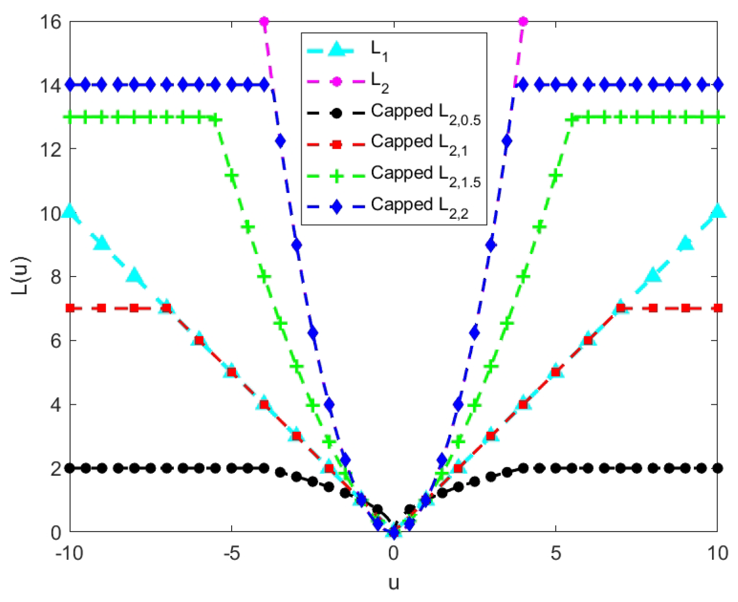
We also provide a comparison of the -norm, the -norm, and the capped -norm (p = 0.5, 1, 1.5, 2) of a scalar in Figure 1. Firstly, from Figure 1, we can see that the -norm and -norm are unbounded, and the capped -norm is bounded. Secondly, we can observe that the capped -norm can be the capped -norm when , and the capped -norm can be the capped -norm when . This indicates that the capped -norm can behave as a capped form of the traditional norm at certain parameter values.
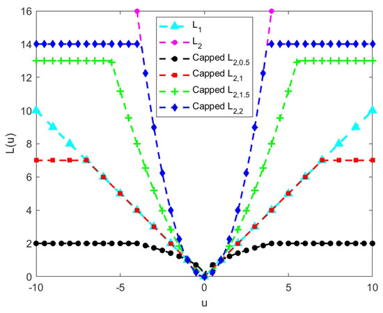
Figure 1.
Comparison of the −norm, the −norm, and the capped −norm with different p values.
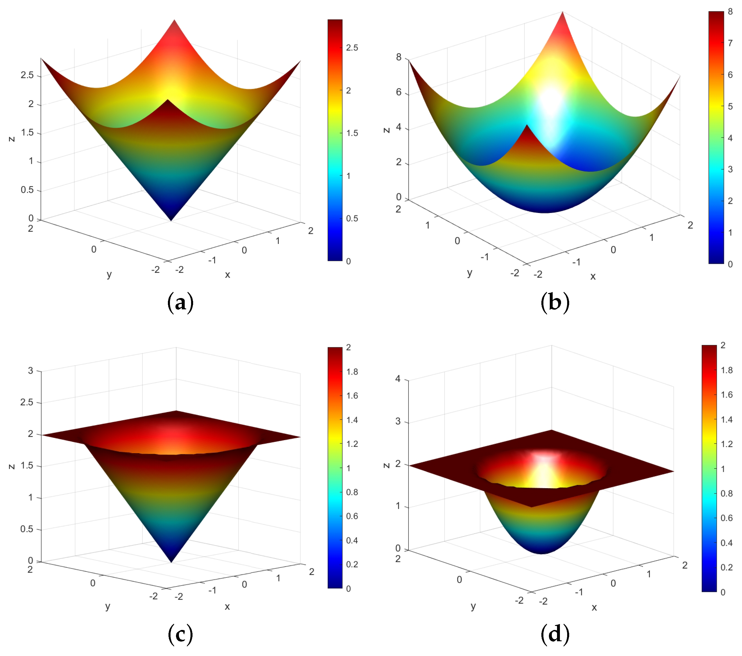
To more intuitively help us understand the characteristics of the capped -norm metric, we also provide a comparison of the -norm and capped -norm for a two-dimensional vector (the high-dimensional situation is similar) as shown in Figure 2. Figure 2a,b are the -norm metric when p takes 1 and 2, respectively, while Figure 2c,d are corresponding capped versions. Figure 2a is an unbounded -norm metric, whose surface is a smooth curve surface. Figure 2b is essentially an unbounded squared -norm metric, which is also a smooth surface, similar to Figure 2a. However, due to the influence of the square, the surface rises rapidly away from the center. Applying it to a model means that it is very sensitive to data points that are far from the center, which can be noise or outliers. Figure 2a also has a relatively sharp turning point, but the overall rise is slow. This norm metric is less sensitive to outliers compared to the squared -norm metric in Figure 2b. Figure 2c,d are the bounded capped -norm metric and capped squared -norm metric, respectively, characterized by flat regions on their surface when the capped threshold is exceeded. If this metric is applied to the model, it can control the impact of the outliers, and the robustness of the model is enhanced.

Figure 2.
Comparison of −norm metric and capped −norm metric: (a) −norm metric (); (b) −norm metric (); (c) capped −norm metric (, ); (d) capped −norm metric (, ).
In conclusion, the capped -norm metric is a better choice when handling datasets containing outliers or noise. Furthermore, the metric can better strengthen the model’s resilience and improve the classification ability of the model.
2.4. Concave-Convex Procedure
The concave-convex procedure (CCCP) [36] is employed to address optimization problems involving the difference of convex functions. Let be the variable; the optimization problem associated with the CCCP is expressed in the following form:
where ; and are realvalued convex functions; and and denote the number of constraints. Suppose that is differentiable. The solution to (14) is derived through an iterative process of solving the subsequent series of convex optimization problems:
3. Squared Fractional Loss Based Robust Supervised Twin Extreme Learning Machine
In this section, we first put forward a new loss function (SF-loss) and then combine it with the TELM, capped -norm metric, and Fisher regularization to propose a new robust supervised learning framework (RS-SFTELM). We also provide a detailed solution process and a convergence analysis for this model.
3.1. Squared Fractional Loss
Convex loss functions ( loss function, loss function, hinge loss function) are commonly utilized in machine learning due to their ability to achieve global optimality. However, their unbounded nature makes them vulnerable to noise and outliers. According to M-estimation theory [34], loss functions with bounded properties or bounded influence functions demonstrate greater robustness to noise and outliers. Thus, we propose a new bounded loss function, called squared fraction loss (abbreviated as SF-loss) in the following:
Definition 1.
Given a vector u, the SF-loss is defined as
where the parameter .
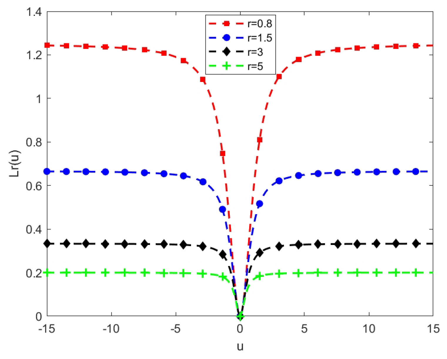
Figure 3 shows the loss function with different parameter r values. From Figure 3, we can see that the parameter r affects the upper bound of the loss function. The more r values, the smaller the upper bounds. In addition, we provide some interesting properties, robustness analysis, and Fisher consistency for our SF-loss function.
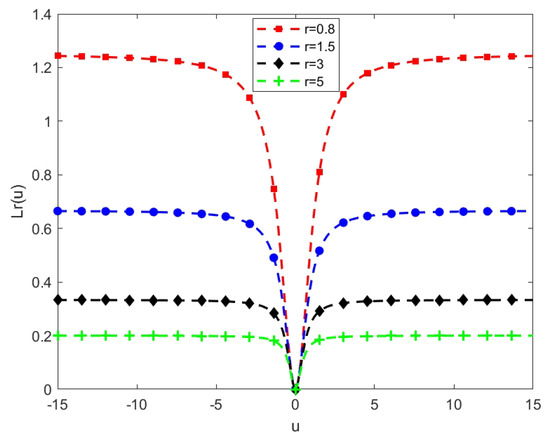
Figure 3.
Loss function with different values of r. The horizontal axis indicates the u value ( is the margin error), while the vertical axis shows the respective loss function value.
3.1.1. The Properties of the SF-Loss Function
Property 1.
= 0 if . This guarantees that the function passes through the original point.
Property 2.
is bounded, which can ensure better robustness.
Proof.
Therefore, is a bounded function. □
Property 3.
is a differentiable function that can help us optimize better.
Proof.
Therefore, is differentiable. □
Property 4.
is a symmetrical function.
Proof.
Calculate and separately and obtain:
Since , is symmetrical. □
Property 5.
is a non-convex function.
Proof.
Let , , , and . Then, we obtain:
Since , i.e., , is a non-convex function. □
3.1.2. Robustness Analysis of SF-Loss Function
Clearly, the new loss function is bounded. From a robust statistics perspective, the shows noise insensitivity, which ensures superior robustness. The derivative of is expressed as:
and we have:
Hence, according to M-estimation theory [34], the loss function is robust against noise.
3.1.3. Fisher Consistency of SF-Loss Function
An important attribute for a binary classifier f: is whether the classifier satisfies Fisher consistency. Specifically, a classifier f is deemed Fisher consistent if the minimizer of the associated expected risk, as dictated by a loss function L, exhibits the same sign as the Bayes classifier [35]. Thus, the loss function L is termed Fisher consistent if it adheres to this property.
In binary classification problems, the training set is represented by , under the assumption that the samples are independent and the probability measure is on . Then, the expected risk of classifier f: is defined as:
Here, denotes the loss function, and represents the conditional probability of the positive (or negative) class when . Under the condition that is given, the conditional distribution of is indicated by . To minimize the expected risk, we introduce the optimization variable q and define the function to minimize the expected risk through the following formula:
where is a function to be optimized to represent the predicted value under a specific condition (i.e., given ). In the binary classification problem, is a binary distribution. Specifically, and denote the probabilities for the positive and negative classes, respectively. The Bayes classifier is given by:
Next, we will examine whether the SF-loss satisfies Fisher consistency.
Property 6.
Function , which minimizes SF-loss expected risk among all measurable functions, is equivalent to the Bayes classifier: . This means that the SF-loss satisfies Fisher consistency.
Proof.
For binary classification, we have:
when and are applied to Formula (16), the following two equations are obtained:
and
Therefore, if , expected risk receives the minimum value when ; if , expected risk receives the minimum value when . Hence, whichever minimizes the expected risk measured by the SF-loss satisfies . This analysis confirms that the minimizer of the associated expected risk, determined by the loss function, has the same sign as the Bayes classifier, thereby proving that this property is satisfied. □
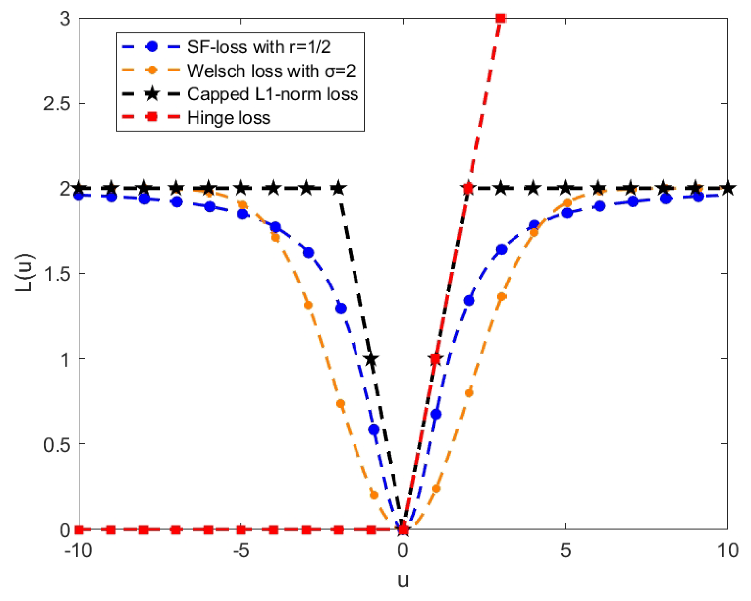
To more clearly compare the performance of our loss function with other advanced loss functions (Hinge loss [20,33], capped -norm loss [25,33], and Welsch loss [30]), we present them in Figure 4. We can observe that the hinge loss is unbounded and tends to exaggerate the impact of outliers. Other losses are bounded, so we set specific parameters to ensure that the upper bounds of these losses are consistent. In this case, our proposed loss function exhibits a smoother characteristic and its growth trend is relatively gradual compared to the capped -norm loss. Compared to the Welsch loss function, our proposed loss function increases rapidly near the origin (corresponding to normal data) and grows relatively slowly further away from it (representing noisy or outlier data points). This characteristic indicates that our loss function places greater emphasis on increasing the loss for normal points, encouraging the model to make more precise predictions for regular data. Meanwhile, due to the slower growth of loss for outliers, the model becomes less sensitive to them, thus reducing their impact and enhancing the overall robustness of the model.
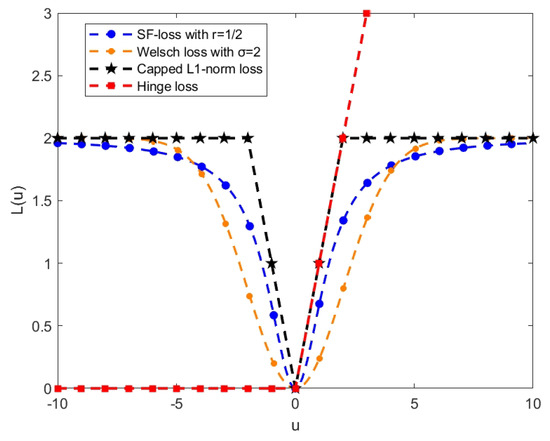
Figure 4.
SF-loss compares hinge loss, capped -norm loss, and Welsch loss. The horizontal axis indicates the u value, while the vertical axis shows the respective loss function value.
3.2. Squared Fractional Loss Based Robust Supervised Twin Extreme Learning Machine
In order to better elaborate on the idea of our model improvement, we rewrite problems (5) and (6) of FTELM as follows:
where hinge loss function , for (32), and for (33), . It is worth noting that FTELM uses the squared -norm metric and hinge loss, which can exaggerate the influence of noise and outliers. To enhance the robustness of the model, we have substituted the squared -norm metric and hinge loss with the capped -norm metric and SF-loss. Therefore, we propose a robust supervised TELM learning framework called SF-loss-based robust supervised TELM (SF-RSTELM). The core problem of our designed model can be described as:
- SF-RSTELM1:
- SF-RSTELM2:where , , , are regularization parameters, and and are the thresholding parameters.
For problem (34), the positive training point approaches the hyperplane as closely as possible by optimizing the first term. Minimizing the second term ensures the negative class samples are as distant as possible from the positive class hyperplane . The last term is the Fisher regularization term that minimizes the intra-class divergence from the samples. For problem (35), a similar interpretation can be applied.
In order to solve the problem effectively, we first work on the first term of the objective function. We first use the concave duality theorem [37] to deal with the first term of the objective functions (34) and (35).
Theorem 1.
Consider a continuous nonconvex function and suppose is a map with range Ω. We assume the existence of a concave function defined on Ω such that is satisfied. Based on this condition, the nonconvex function can be represented as:
Following concave duality [38], is the concave dual of given as:
Furthermore, the minimum on the right-hand side of (36) is obtained at :
According to Theorem 1, we define a concave function such that :
Suppose . The capped -norm metric can be reformulated as:
where . Therefore, the capped -norm metric can also be represented as:
The is the concave dual of , represented as:
By optimizing for (44), we can obtain:
Therefore, the capped -norm metric can be further converted to:
where
Similarly, let . is represented as a concave dual function of , so the capped -norm metric can be written as:
where
Let , and we can obtain:
Similarly, let , and we can obtain:
When the variables and are fixed to solve the classifier-related parameters and , the optimization problems (34) and (35) can be written as:
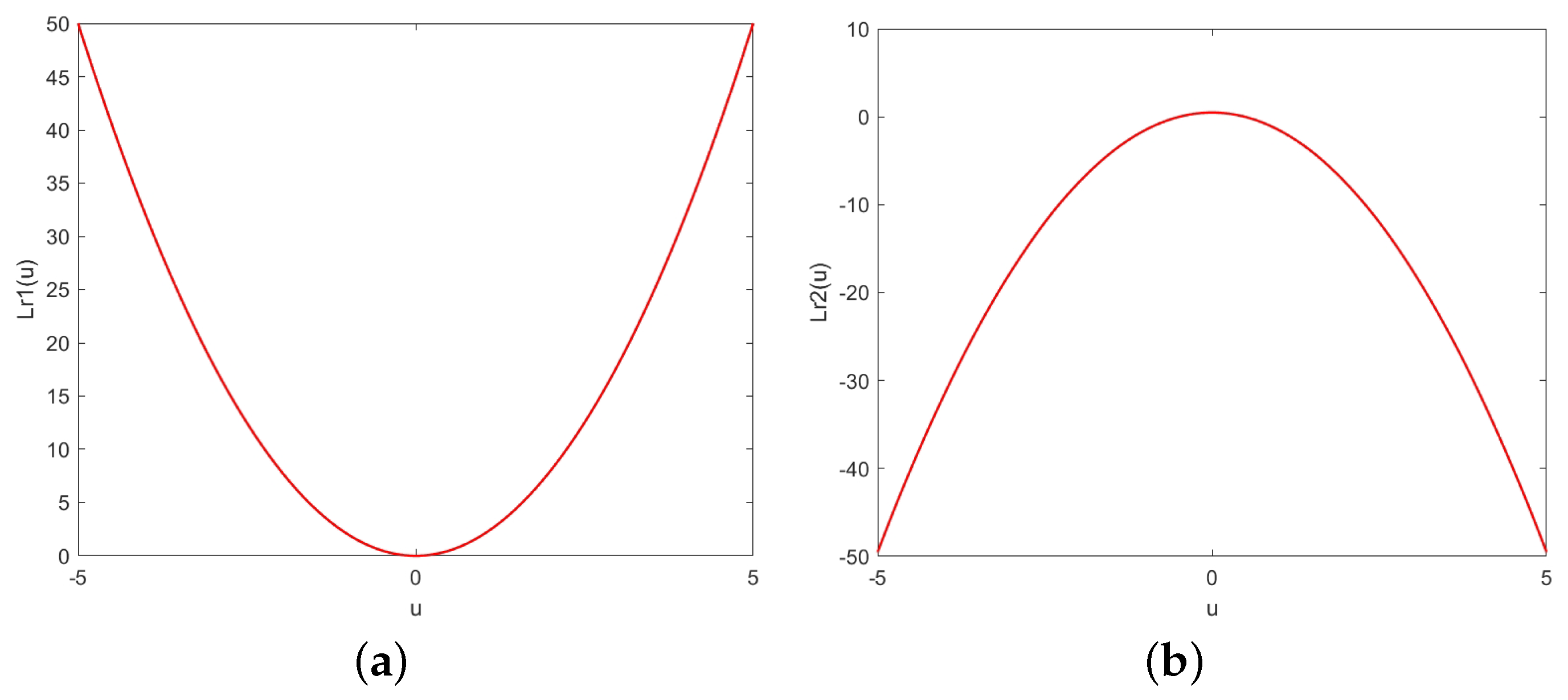
It can be seen that (57) and (58) are non-convex optimization problems because of the non-convexity of the loss function. In this research, we utilize the CCCP technique to handle the non-convexity. Note that the loss function can be expressed as the subtraction of two convex functions, or equivalently, as the sum of a convex function and a concave function. That is, . The specific expressions for the convex function and the concave function are:
Figure 5 represents the graphs for and .
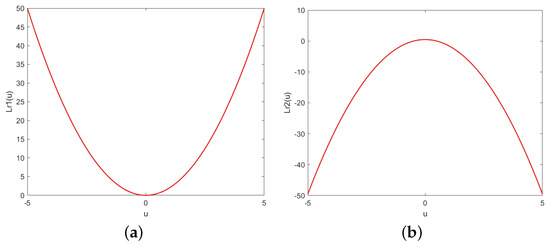
Figure 5.
Convex function (a) and concave function (b) .
Therefore, the above optimization problem can be expressed as:
Since (61) and (62) are similar, we will only show the solution process for (61), which can also be expressed as:
The solution to the above optimization issue can be obtained by addressing the following equation:
The value of in iterations is as follows:
Let , where .
where . Therefore, we can get:
Solving (65) is equivalent to solving the following subproblem:
Here, we introduce Lagrange multipliers for problem (68). Next, its Lagrange function is given by:
Following the Karush–Kuhn–Tucker (KKT) conditions, we derive the following constraints:
From the KKT condition, we can obtain:
Using a similar approach, we can obtain the dual problem of Equation (58):
Therefore, the decision function of SF-RSTELM is given by:
Based on the previous discussion, we provide a detailed description of the implementation steps of the proposed method in Algorithm 1.
| Algorithm 1 The procedure of SF-RSTELM |
| Input: The training set , where and ; |
| Parameters , , , and , , , , . ,. |
| Activation function ; The number of hidden nodes L. |
| Maximum number of iterations . |
| Output:, . |
| Step: |
| 1: Initialize and ; and |
| 2: Compute the graph matrix , . |
| 3: Set . |
| 4: While |
| Calculate and for the dual problem (72) and (73), respectively. |
| Then get the solution , by |
| Update the matrices , , and by (51), (52) and (66). |
| if or |
| break |
| else |
| end while |
| 5: Construct the following decision functions: |
3.3. Convergence Analysis
Theorem 2.
Utilizing the CCCP technique to address problem (63), the resulting sequence converges.
Proof of Theorem 2.
At the iteration point of step , the following inequality holds:
It can be written as
Due to the concavity of , we have
By combining the above inequalities, we have
Accordingly, the objective value of problem (63) decreases monotonically with each iteration and remains non-negative, thereby proving the convergence of the sequence. □
Proof of Theorem 3.
First and foremost, let us recall the formulation of our framework, namely Equation (34).
For convenience, let and . When , we represent the Lagrange function of (81) as follows:
Then, we differentiate with respect to :
According to (51), we bring into Formula (83):
Similarly, we obtain the Lagrangian function of problem (55):
Taking the derivative of with respect to :
It is noted that Formula (84) is equal to Formula (86) when determining the optimal solution . Furthermore, the optimal solution meets the KKT condition of model (34). By solving problem (55), we can determine the optimal solution for problem (34). Thus, Algorithm 1 is capable of converging to a local optimum, making it feasible to obtain the local minimum of problem (34). □
4. Numerical Experiments
Within this part, we performed a comparison of SF-RSTELM with several algorithms, such as TELM [20], FTELM [33], -FTELM [33], FRTELM [25], and CWTELM [30]. To assess the performance of the proposed algorithm, experiments are carried out on four distinct types of databases: artificial datasets, UCI datasets, image datasets, and NDC large datasets. In addition, we demonstrate the convergence of the proposed algorithm through experimental analysis.
4.1. Experimental Setting
4.1.1. Operating Environment
All experiments were carried out using MATLAB (2021a) (MathWorks, Natick, United States) on a personal computer (PC) equipped with an Intel Core-i7 processor (2.5 GHz) and 16 GB random-access memory (RAM).
4.1.2. Benchmark Approaches
We have selected five advanced algorithms as benchmarks to compare with the SF-RSTELM proposed in this paper. These algorithms are:
- TELM [20]: Using the hinge loss function and squared -norm metric.
- FTELM [33]: The Fisher regularization term is introduced into TELM, and relates to the statistical information of intra-class samples.
- -FTELM [33]: Capped -norm loss and metric are introduced into FTELM.
- FRTELM [25]: Capped -norm loss and metric are introduced into TELM.
- CWTELM [30]: Replace the hinge loss function and squared -norm metric in TELM with Welsch loss function and capped -norm metric.
4.1.3. Parameter Selection
In the training process of the model, the selection of parameters is crucial because it will affect the classification performance of the model. Here are some parameters that are respectively required for each model. Since both the comparison model and our model are twin models, which contain two optimization problems, the two optimization models are carried out separately. Therefore, with regard to the parameter selection problem, we will only explain the parameter selection method for one of the optimization problems, and the other model is similar.
- TELM: the count of hidden layer nodes L, the regularization parameter .
- FTELM: the count of hidden layer nodes L, the regularization parameters , .
- -FTELM: the count of hidden layer nodes L, the regularization parameters , , the capped parameter in the metric, and the capped parameter in the loss function.
- FRTELM: the count of hidden layer nodes L, the regularization parameter , the capped parameter in the metric, and the capped parameter in the loss function.
- CWTELM: the count of hidden layer nodes L, the regularization parameter , the capped parameters and the parameter p of the metric, and the parameter in the loss function.
- SF-RSTELM: the count of hidden layer nodes L, the regularization parameters , , the capped parameters and the parameter p of capped -norm metric, and the parameter r in the loss function.
Due to the different number of parameters in different models, we will adopt different parameter selection strategies. For models with fewer than three parameters (TELM and FTELM), we will use grid search and ten-fold cross-validation to explore the parameter space and find the optimal parameter combination. However, when dealing with models with more than three parameters (-FTELM, FRTELM, CWTELM, and SF-RSTELM), directly applying grid search may lead to a significant increase in computational load. To overcome this challenge, we first fix some parameters to narrow down the search space based on initial experimental results and domain expertise. The fixed parameter strategy is as follows: the count of hidden nodes L is fixed, but L should be different for different datasets, and the range of L is . For a fair contrast, we fix the parameters to ensure that the above algorithms with bounded loss functions have the same upper bound on their loss. Specifically, we set the capped -norm loss parameter to 2 in -FTELM and FRTELM, the parameter to 2 in CWTELM for Welsch loss, and the parameter r to 0.5 in our model’s SF-loss. Moreover, for the aforementioned models that utilize bounded metrics, we set all their upper bounds to be equal. That is, the capped parameter is set to 0.001. In addition to fixing the above parameters, we still choose to use ten-fold cross-validation and grid search to find the best values for the remaining parameters. Specifically, the regularization parameters and are chosen from , and the parameter p is chosen from .
4.1.4. Evaluation Criteria
To assess the validity of the model, we employ accuracy () and the -score as evaluation criteria. Specifically, these criteria are specified as follows:
where , , , and refer to true positives, true negatives, false positives, and false negatives, respectively. Both and the -score serve to evaluate the model’s generalization capability, and the higher they are, the better the performance. To guarantee the reliability of our experiments, we repeat all experimental procedures 10 times, and the final experimental result is the mean of the 10 repetitions.
4.2. Experiments on the Artificial Datasets
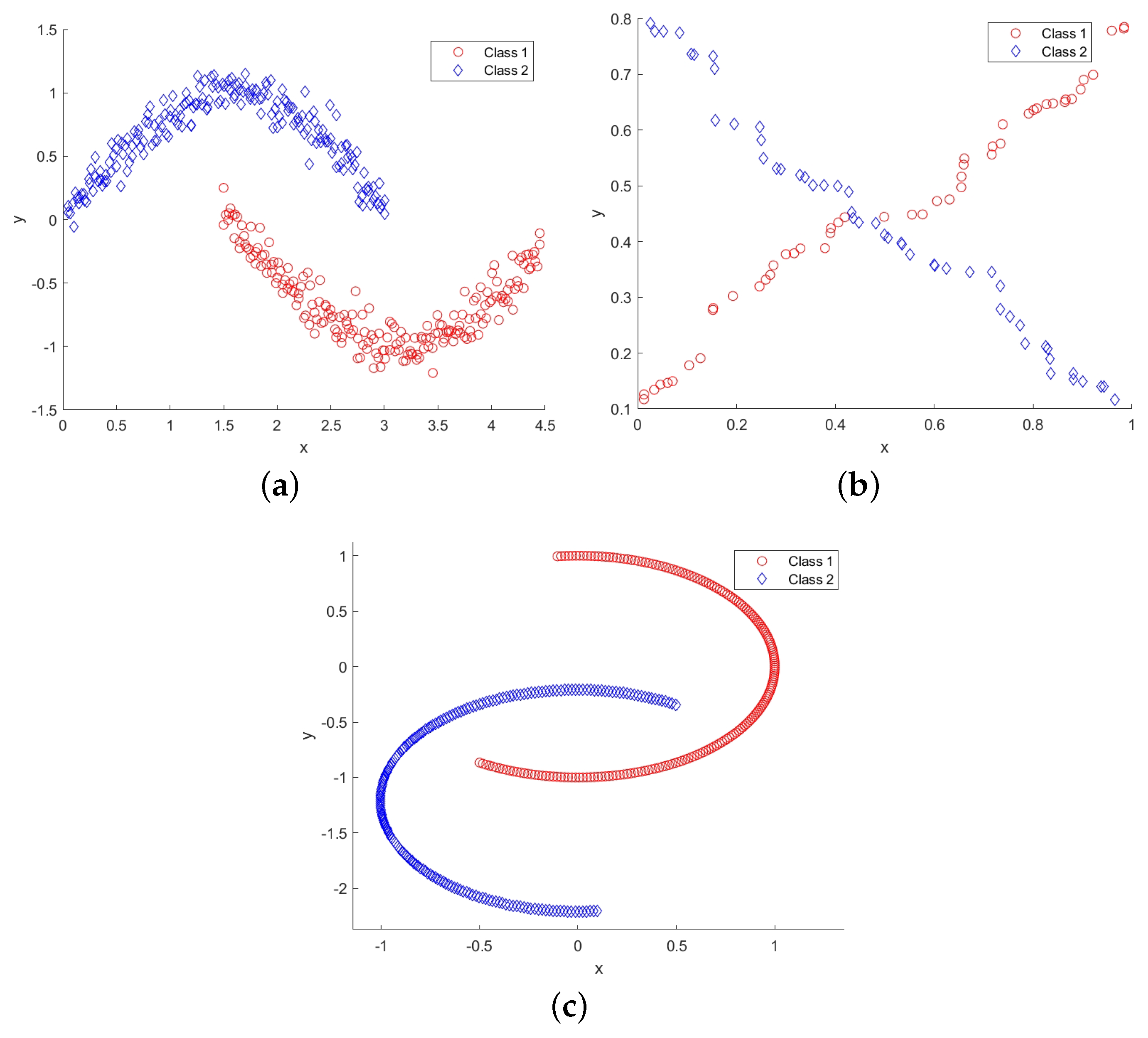
In this subsection, experiments are initially performed on the Two Moons, XOR, and Banana datasets. Both the Two Moons and Banana datasets comprise 400 samples, while the XOR dataset contains 100 samples. Figure 6 visually depicts the two-dimensional distribution graphs of these three artificial datasets. Class 1 is shown as a red ‘∘’, and class 2 is shown as a blue ‘⋄’.

Figure 6.
Two dimensional distribution graphs of three artificial datasets (Two Moons, XOR, Banana): (a) Two Moons; (b) XOR; (c) Banana.
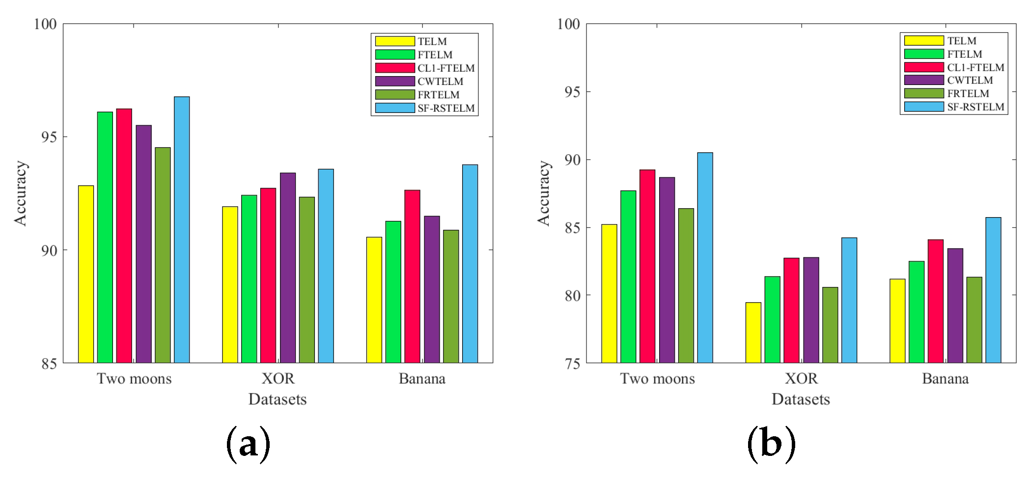
To test the performance of the proposed method, Figure 7 shows the accuracy of five comparison algorithms as well as the proposed algorithm under conditions of no noise and a noise ratio of 20%. The noise is introduced by randomly selecting training samples and perturbing their features with Gaussian noise that follows a normal distribution . Specifically, for the training data X, is used instead of X, where represents the noise matrix that adheres to a normal distribution with a mean of 0 and a variance of .

Figure 7.
Experimental results of six algorithms on three artificial datasets: (a) experimental results of six algorithms on three artificial datasets without noise; (b) experimental results of six algorithms on three artificial datasets with 20% noise.
As can be seen from Figure 7a, the accuracy of SF-RSTELM is highest among the six methods when no noise is added to the dataset. Our model has the highest accuracy, which can be explained in three ways. First, it uses a bounded capped -norm metric, whose p-value can be flexibly adjusted to suit different data. Second, we use a bounded loss that effectively controls the upper bound. In addition, we consider the intra-class divergence information of the data. The remaining algorithms are sorted in descending order of accuracy as -FTELM, CWTELM, FTELM, FRTELM, TELM. The accuracy of -FTELM is slightly lower than that of our model, probably because the capped -norm metric is not as flexible as the capped -norm metric we use. Although CWTELM has also improved the metric and loss, it still falls slightly below -FTELM due to its failure to consider the statistical properties of the data. FTELM is merely an extension of TELM, with the addition of a Fisher regularization term. FRTELM improved the metric and loss; however, the intra-class divergence information of the data is not taken into account. When noise is added to the dataset (Figure 7b), the performance of all algorithms is degraded, but SF-RSTELM’s accuracy is still the highest. This shows that our algorithm has the strongest noise immunity and robustness.
4.3. Experiments on the UCI Datasets
In this subsection, we evaluate the performance of our model on nine UCI datasets from http://archive.ics.uci.edu/ml/datasets.php (accessed on 15 February 2024) and contrast it with five other state-of-the-art algorithms. Table 1 provides a detailed overview of the characteristics of the UCI datasets employed. All features within these datasets are normalized to a scale of to ensure consistency.

Table 1.
Characteristics of UCI datasets.
Initially, we assess the steadiness of our SF-RSTELM without adding extra noises. Table 2 presents the results of the experiments, with the best results highlighted in bold. Here, Time(s) denotes the average execution time for each algorithm when optimized with the best parameters. In ACC ± S, ACC denotes the mean learning accuracy, while S represents the standard deviation. Table 2 shows that SF-RSTELM outperforms the other five methods in terms of accuracy and on most datasets, except for the German, Pima, and QSAR datasets. This is because SF-RSTELM not only incorporates the Fisher regularization term, which considers intra-class divergence, but also leverages the parameter adjustability of SF-loss and the flexibility of the capped -norm metric.
Table 2.
Experimental results on UCI datasets. The best results are marked in bold.
Moreover, to illustrate the noise-resistant properties of SF-RSTELM, we introduce Gaussian noise into the training subset, affecting their features to generate noise. The experimental outcomes at noise levels of 15% and 25% are displayed in Table 3 and Table 4. It is clear that with rising noise levels, the learning accuracy of all algorithms declines. However, SF-RSTELM maintains higher accuracy and scores compared to the other five methods, except on a few datasets. This also demonstrates the strong noise resistance capability of our model.
Table 3.
Experimental results on UCI datasets with 15% Gaussian noise. The best results are marked in bold.
Table 4.
Experimental results on UCI datasets with 25% Gaussian noise. The best results are marked in bold.
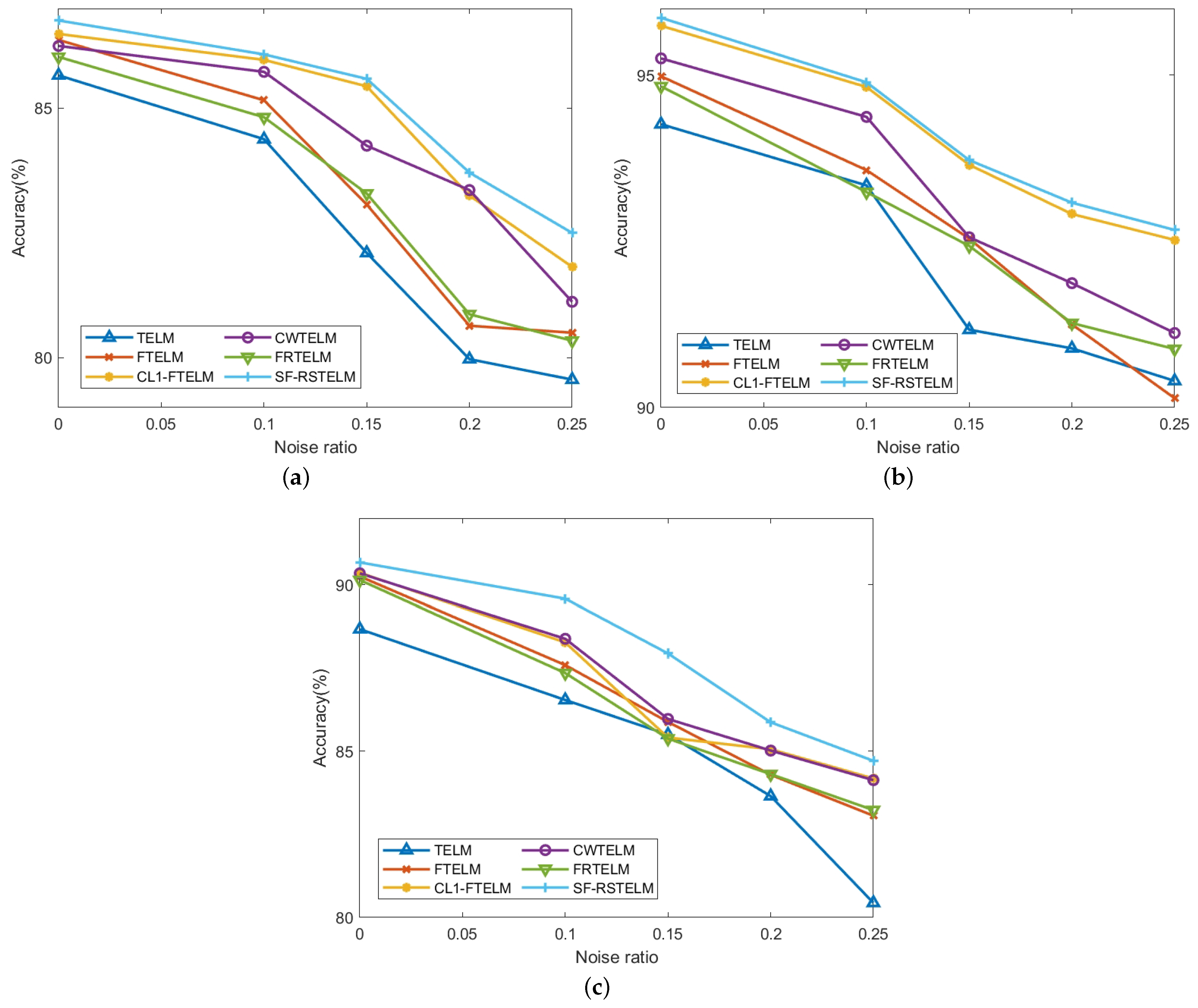
To demonstrate the robustness of SF-RSTELM at varying noise levels (10%, 15%, 20%, and 25%), experiments are conducted on three datasets (Australian, Vote, and Ionosphere). Figure 8 illustrates the accuracy variation line charts of six algorithms on these three datasets across different noise levels. For the original dataset , we change it with , where is the Gaussian variable. Here, , and is a noise ratio. The value of . As is evident from Figure 8, the performance of all algorithms decreases as noise levels rise, but the accuracy of our model decreases the slowest. This further indicates that SF-RSTELM possesses superior classification accuracy compared to the other five methods. This superiority in noise handling is likely attributed to the combined effectiveness of the SF-loss function, the capped -norm metrics, and the Fisher regularization term.
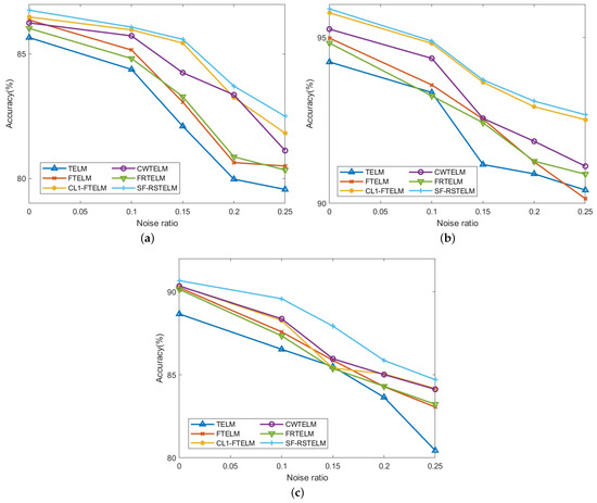
Figure 8.
Under different noise ratios, the accuracy variation curves of six algorithms across three datasets: (a) Australian; (b) Vote; (c) Ionosphere.
4.4. Experiments on the Image Datasets
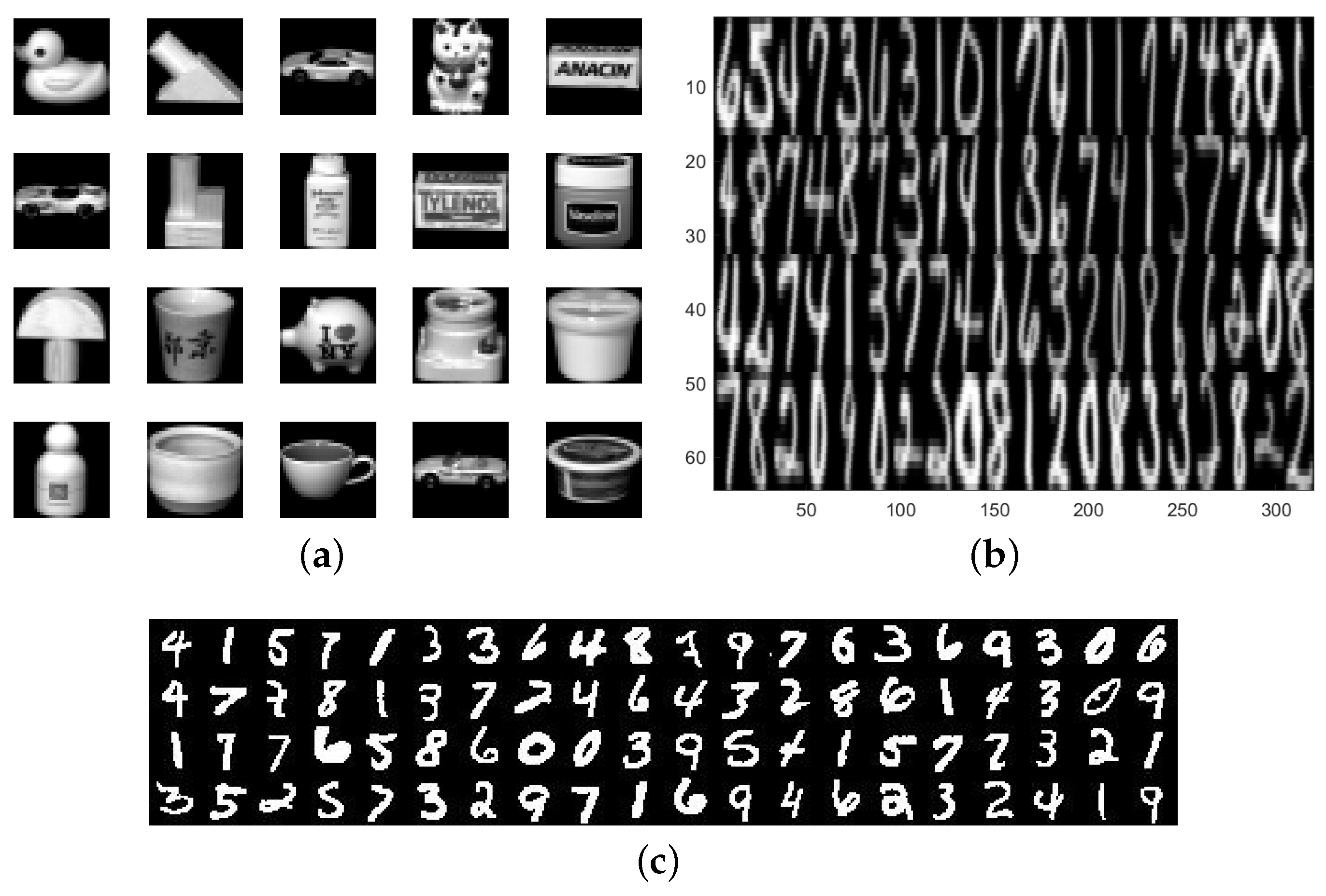
In this part, we will perform experiments using high-dimensional image datasets to assess and compare the noise resistance and classification accuracy of our model SF-RSTELM with five other algorithms. We utilized the following three image datasets: COIL-20 http://www.cad.zju.edu.cn/home/dengcai/Data/FaceData.html (accessed on 15 February 2024), USPS http://www.cad.zju.edu.cn/home/dengcai/Data/FaceData.html (accessed on 15 February 2024), and MNIST http://www.cad.zju.edu.cn/home/dengcai/Data/FaceData.html (accessed on 15 February 2024). Since these image datasets are essentially a problem with multiple classes, we employed the “one-vs-rest” strategy to convert them to multiple binary classification problems. Table 5 shows the features of the three image datasets. Figure 9 demonstrates examples from the three high-dimensional image datasets. Specifically, due to the large size of the MNIST dataset, we only select the first 2000 samples to participate in the experiment. These image datasets are utilized to evaluate the performance of our models in multi-class classification tasks.
Table 5.
Characteristics of image datasets.
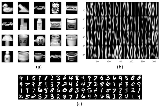
Figure 9.
Example images for three image datasets: (a) COIL-20 database; (b) USPS database; (c) MNIST database.
The specific experimental results are presented in Table 6. From the experiment results, it is evident that SF-RSTELM has the highest accuracy on all three datasets. Table 7 shows the results after adding 15% Gaussian noise. It can be seen that the ACC and value of all models are significantly reduced, but our model is still the highest, which also indicates that our model has good noise resistance capability, classification ability, and ability to process high-dimensional image datasets.
Table 6.
Experimental results on image datasets. The best results are marked in bold.
Table 7.
Experimental results on image datasets with 15% Gaussian noise. The best results are marked in bold.
4.5. Experiments on the NDC Large Datasets
In this subsection, to evaluate the stability of our proposed model on large-scale datasets. We have conducted a comparative analysis of our algorithm with five other algorithms using the NDC datasets generated by David Musicant’s NDC data generator http://www.cs.wisc.edu/musicant/data/ndc (accessed on 15 February 2024). Detailed descriptions of the NDC datasets are presented in Table 8. Table 9 summarizes the experimental results of the six algorithms on three large-scale NDC datasets.
Table 8.
Characteristics of NDC datasets.
Table 9.
Experimental results on NDC large datasets. The best results are marked in bold.
As can be seen from Table 9, our model SF-RSTELM has the highest accuracy and value except for the NDC-15k dataset. Overall, SF-RSTELM is more stable than the other five algorithms. This is mainly due to the advantages of SF-RSTELM, which not only incorporates the statistical attributes of the data, but also uses the bounded and flexibly adjustable metric and loss function, which effectively controls the disturbance from noise and outliers. Therefore, from this set of experimental results, we can see that our model is also effective for large datasets.
4.6. Convergence Curve
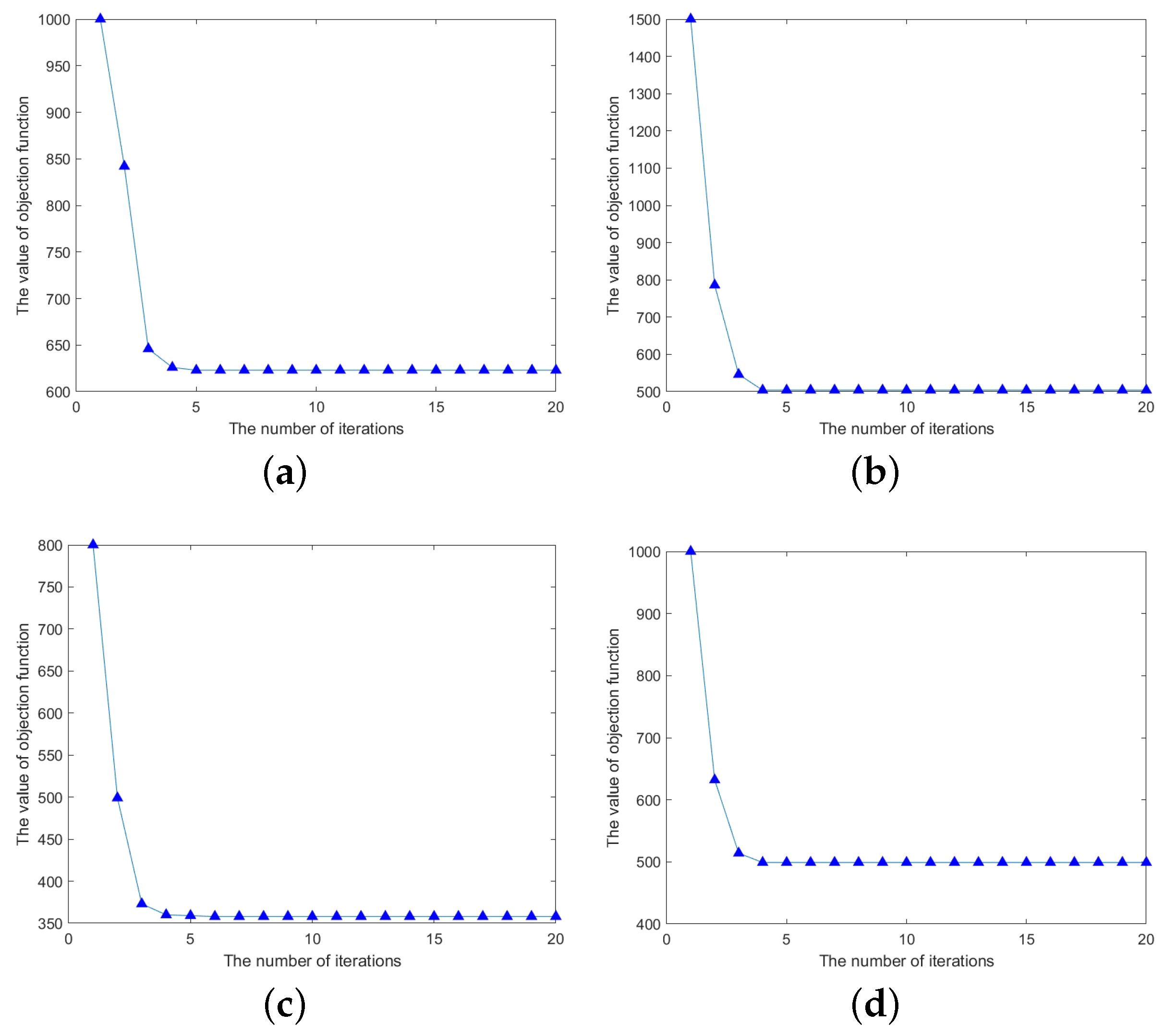
We also perform experiments on four UCI datasets (Australian, QSAR, WDBC, and Vote) to confirm the convergence of the proposed Algorithm 1. Figure 10 demonstrates the convergence case of the objective function value with the increasing number of iterations. As can be seen from Figure 10, the objective function value converges relatively quickly to a stable fixed value.
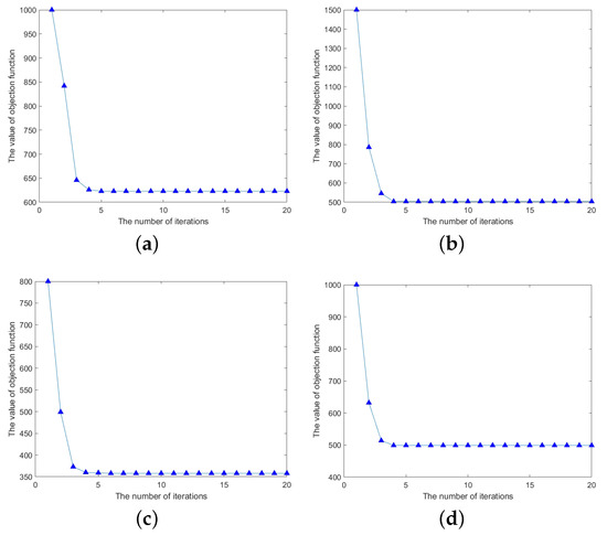
Figure 10.
Convergence graph of SF-RSTELM’s objective function values increasing with the number of iterations on four datasets (Australian, QSAR, WDBC, Vote): (a) Australian; (b) QSAR; (c) WDBC; (d) Vote.
This observation verifies the effectiveness of our algorithm in converging the objective function to a local optimum within a finite number of iterations, thereby demonstrating its convergence properties.
5. Conclusions and Future Works
In this paper, we first propose a new kind of SF-loss function that exhibits favorable characteristics including boundedness, smoothness, symmetry, noise insensitivity, and Fisher consistency. Then, SF-RSTELM is proposed by integrating the capped -norm metric, SF-loss, and Fisher regularization term. SF-RSTELM not only integrates the Fisher regularization term, addressing the intra-class divergence of the data, but also exploits the parameter adjustability of SF-loss and the flexibility of capped -norm metrics to reduce the influence of noise and outliers. Moreover, an efficient iterative algorithm is proposed to solve the model, and the convergence of the algorithm is proved. Experimental results on multiple datasets demonstrate the efficiency of the proposed model. Specifically, our model was able to achieve higher ACC and scores on most datasets, with improvements ranging from 0.28% to 4.5% compared to other state-of-the-art algorithms.
In the future, we will continue to study the improvement of the algorithm. Because the model constructed in this paper represents a non-convex optimization problem, we convert it into a series of convex problems to solve by the CCCP method, resulting in a long training time, so it is necessary to find a fast solution method in future research. Moreover, transforming this paper’s model from supervised to semi-supervised learning remains an important direction for future studies.
Author Contributions
Z.X., conceptualization, methodology, validation, investigation, project administration, writing—original draft. Y.W., methodology, software, validation, formal analysis, investigation, data curation, writing—original draft. Y.R., validation, software. X.Z., validation, software. All authors have read and agreed to the published version of the manuscript.
Funding
The authors wish to acknowledge the financial support of the National Nature Science Youth Foundation of China (No. 61907012), Construction Project of First-Class Disciplines in Ningxia Higher Education (NXYLXK2017B09), Postgraduate Innovation Project of North Minzu University (YCX23098, YCX23091), National Nature Science Foundation of China (No. 62366001), and the Natural Science Foundation of Ningxia (2024A2787).
Informed Consent Statement
The authors declare that they have no known competing financial interests or personal relationships that could have appeared to influence the work reported in this paper.
Data Availability Statement
The UCI machine learning repository is available at http://archive.ics.uci.edu/ml/datasets.php (accessed on 15 February 2024). The image data are available at http://www.cad.zju.edu.cn/home/dengcai/Data/FaceData.html (accessed on 15 February 2024). The NDC datasets are available at http://www.cs.wisc.edu/musicant/data/ndc. (accessed on 15 February 2024).
Acknowledgments
The authors thank the anonymous reviewers for their constructive comments.
Conflicts of Interest
The authors declare no conflicts of interest.
References
- Sakheta, A.; Raj, T.; Nayak, R.; O’Hara, I.; Ramirez, J. Improved prediction of biomass gasification models through machine learning. Comput. Chem. Eng. 2024, 191, 108834. [Google Scholar] [CrossRef]
- Maydanchi, M.; Ziaei, M.; Mohammadi, M.; Ziaei, A.; Basiri, M.; Haji, F.; Gharibi, K. A Comparative Analysis of the Machine Learning Methods for Predicting Diabetes. J. Oper. Intell. 2024, 2, 230–251. [Google Scholar] [CrossRef]
- Kim, E.; Yang, S.M.; Ham, J.H.; Lee, W.; Jung, D.H.; Kim, H.Y. Integration of MALDI-TOF MS and machine learning to classify enterococci: A comparative analysis of supervised learning algorithms for species prediction. Food Chem. 2024, 462, 140931. [Google Scholar] [CrossRef]
- Ding, S.; Zhao, H.; Zhang, Y.; Xu, X.; Nie, R. Extreme learning machine: Algorithm, theory and applications. Artif. Intell. Rev. 2015, 44, 103–115. [Google Scholar] [CrossRef]
- Deng, C.; Huang, G.; Xu, J.; Tang, J. Extreme learning machines: New trends and applications. Sci. China Inf. Sci. 2015, 2, 1–16. [Google Scholar] [CrossRef]
- Huang, G.B.; Zhu, Q.Y.; Siew, C.K. Extreme learning machine: Theory and applications. Neurocomputing 2006, 70, 489–501. [Google Scholar] [CrossRef]
- Mirza, B.; Kok, S.; Dong, F. Multi-layer online sequential extreme learning machine for image classification. In Proceedings of the ELM-2015 Volume 1: Theory, Algorithms and Applications (I), Hangzhou, China, 15–17 December 2015; Springer: Berlin/Heidelberg, Germany, 2016; pp. 39–49. [Google Scholar]
- Yu, H.; Yuan, K.; Li, W.; Zhao, N.; Chen, W.; Huang, C.; Chen, H.; Wang, M. Improved butterfly optimizer-configured extreme learning machine for fault diagnosis. Complexity 2021, 2021, 1–17. [Google Scholar] [CrossRef]
- Chen, Z.; Gryllias, K.; Li, W. Mechanical fault diagnosis using convolutional neural networks and extreme learning machine. Mech. Syst. Signal Process. 2019, 133, 106272. [Google Scholar] [CrossRef]
- Wang, Z.; Li, M.; Wang, H.; Jiang, H.; Yao, Y.; Zhang, H.; Xin, J. Breast cancer detection using extreme learning machine based on feature fusion with CNN deep features. IEEE Access 2019, 7, 105146–105158. [Google Scholar] [CrossRef]
- Zhu, W.; Miao, J.; Hu, J.; Qing, L. Vehicle detection in driving simulation using extreme learning machine. Neurocomputing 2014, 128, 160–165. [Google Scholar] [CrossRef]
- Deeb, H.; Sarangi, A.; Mishra, D.; Sarangi, S.K. Human facial emotion recognition using improved black hole based extreme learning machine. Multimed. Tools Appl. 2022, 81, 24529–24552. [Google Scholar] [CrossRef]
- Zhou, J.; Zhang, X.; Jiang, Z. Recognition of imbalanced epileptic EEG signals by a graph-based extreme learning machine. Wirel. Commun. Mob. Comput. 2021, 2021, 1–12. [Google Scholar] [CrossRef]
- Zhao, J.; Xu, Y.; Fujita, H. An improved non-parallel universum support vector machine and its safe sample screening rule. Knowl.-Based Syst. 2019, 170, 79–88. [Google Scholar] [CrossRef]
- Sun, F.; Xie, X. Deep Non-Parallel Hyperplane Support Vector Machine for Classification. IEEE Access 2023, 11, 7759–7767. [Google Scholar] [CrossRef]
- Chen, S.; Cao, J.; Huang, Z. Weighted linear loss projection twin support vector machine for pattern classification. IEEE Access 2019, 7, 57349–57360. [Google Scholar] [CrossRef]
- Zheng, X.; Zhang, L.; Yan, L. Sparse discriminant twin support vector machine for binary classification. Neural Comput. Appl. 2022, 34, 16173–16198. [Google Scholar] [CrossRef]
- Borah, P.; Gupta, D. Robust twin bounded support vector machines for outliers and imbalanced data. Appl. Intell. 2021, 51, 5314–5343. [Google Scholar] [CrossRef]
- Xiao, Y.; Liu, J.; Wen, K.; Liu, B.; Zhao, L.; Kong, X. A least squares twin support vector machine method with uncertain data. Appl. Intell. 2023, 53, 10668–10684. [Google Scholar] [CrossRef]
- Wan, Y.; Song, S.; Huang, G.; Li, S. Twin extreme learning machines for pattern classification. Neurocomputing 2017, 260, 235–244. [Google Scholar] [CrossRef]
- Wang, C.; Ye, Q.; Luo, P.; Ye, N.; Fu, L. Robust capped L1-norm twin support vector machine. Neural Netw. 2019, 114, 47–59. [Google Scholar] [CrossRef]
- Wang, Y.; Yu, G.; Ma, J. Capped linex metric twin support vector machine for robust classification. Sensors 2022, 22, 6583. [Google Scholar] [CrossRef] [PubMed]
- Kumari, A.; Tanveer, M.; Alzheimer’s Disease Neuroimaging Initiative. Universum twin support vector machine with truncated pinball loss. Eng. Appl. Artif. Intell. 2023, 123, 106427. [Google Scholar] [CrossRef]
- Ma, J.; Yang, L.; Sun, Q. Adaptive robust learning framework for twin support vector machine classification. Knowl.-Based Syst. 2021, 211, 106536. [Google Scholar] [CrossRef]
- Ma, J. Capped L1-norm distance metric-based fast robust twin extreme learning machine. Appl. Intell. 2020, 50, 3775–3787. [Google Scholar] [CrossRef]
- Yang, Y.; Xue, Z.; Ma, J.; Chang, X. Robust projection twin extreme learning machines with capped L1-norm distance metric. Neurocomputing 2023, 517, 229–242. [Google Scholar] [CrossRef]
- Ma, J.; Yang, L. Robust supervised and semi-supervised twin extreme learning machines for pattern classification. Signal Process 2021, 180, 107861. [Google Scholar] [CrossRef]
- Yuan, C.; Yang, L. Capped L2,P-norm metric based robust least squares twin support vector machine for pattern classification. Neural Netw. 2021, 142, 457–478. [Google Scholar] [CrossRef]
- Wang, H.; Yu, G.; Ma, J. Capped L2,P-Norm Metric Based on Robust Twin Support Vector Machine with Welsch Loss. Symmetry 2023, 15, 1076. [Google Scholar] [CrossRef]
- Jiang, Y.; Yu, G.; Ma, J. Distance Metric Optimization-Driven Neural Network Learning Framework for Pattern Classification. Axioms 2023, 12, 765. [Google Scholar] [CrossRef]
- Ma, J.; Wen, Y.; Yang, L. Fisher-regularized supervised and semi-supervised extreme learning machine. Knowl. Inf. Syst. 2020, 62, 3995–4027. [Google Scholar] [CrossRef]
- Xue, Z.; Zhao, C.; Wei, S.; Ma, J.; Lin, S. Robust Fisher-regularized extreme learning machine with asymmetric Welsch-induced loss function for classification. Appl. Intell. 2024, 54, 7352–7376. [Google Scholar] [CrossRef]
- Xue, Z.; Cai, L. Robust Fisher-Regularized Twin Extreme Learning Machine with Capped L1-Norm for Classification. Axioms 2023, 12, 717. [Google Scholar] [CrossRef]
- Huber, P.J. Robust estimation of a location parameter. In Breakthroughs in Statistics: Methodology and Distribution; Springer: Berlin/Heidelberg, Germany, 1992; pp. 492–518. [Google Scholar]
- Yuan, C.; Yang, L. Robust twin extreme learning machines with correntropy-based metric. Knowl.-Based Syst. 2021, 214, 106707. [Google Scholar] [CrossRef]
- Yuille, A.L.; Rangarajan, A. The concave-convex procedure. Neural Comput. 2003, 15, 915–936. [Google Scholar] [CrossRef] [PubMed]
- Zhang, T. Analysis of multi-stage convex relaxation for sparse regularization. J. Mach. Learn. Res. 2010, 11, 1081–1107. [Google Scholar]
- Rockafellar, R. Convex Analysis. Princet. Math. Ser. 1970, 28, 326–332. [Google Scholar]
Disclaimer/Publisher’s Note: The statements, opinions and data contained in all publications are solely those of the individual author(s) and contributor(s) and not of MDPI and/or the editor(s). MDPI and/or the editor(s) disclaim responsibility for any injury to people or property resulting from any ideas, methods, instructions or products referred to in the content. |
© 2024 by the authors. Licensee MDPI, Basel, Switzerland. This article is an open access article distributed under the terms and conditions of the Creative Commons Attribution (CC BY) license (https://creativecommons.org/licenses/by/4.0/).