On a Randomly Censoring Scheme for Generalized Logistic Distribution with Applications

Abstract

In this paper, we investigate the inferential procedures within both classical and Bayesian frameworks for the generalized logistic distribution under a random censoring model. For randomly censored data, our main goals were to develop maximum likelihood estimators and construct confidence intervals using the Fisher information matrix for the unknown parameters. Additionally, we developed Bayes estimators with gamma priors, addressing both squared error and general entropy loss functions. We also calculated Bayesian credible intervals for the parameters. These methods were applied to two real datasets with random censoring to provide valuable insights. Finally, we conducted a simulation analysis to assess the effectiveness of the estimated values.

1. Introduction

Obtaining a complete dataset can be difficult since time and financial restrictions frequently limit data collection. The term ’censored data’ refers to these incomplete data. A variety of censoring techniques for studying such data are available in the literature. Type I and Type II censoring are the most commonly employed techniques. In Type I censoring, an event is only observed if it happens before a predetermined time. On the other hand, Type II censoring continues until a certain number of events of interest have been observed.

Random censoring is a widely discussed technique in the literature. It occurs when a study subject is lost or withdrawn from an experiment before the event of interest takes place. In medical time-to-event studies, such as clinical trials, random censoring is commonly used because some patients may discontinue treatment and leave the study before its conclusion. Consequently, their data are considered to be randomly censored. The concept of random censoring was first introduced in Gilbert’s [1] dissertation. For further detailed information on censoring methods, their generalizations, and analysis, one can refer to the works of [2,3,4,5,6,7,8,9,10,11,12,13,14,15,16,17,18,19].

Logistic distribution is heavy-tailed and symmetric, making it unsuitable for handling asymmetric or thin-tailed data. To address this limitation, the logistic distribution can be extended to include both symmetric and asymmetric data with either heavy or thin tails. One such extension is generalized logistic (GL) distribution, as established by Balakrishnan and Leung [20]. The GL distribution can accommodate a wider range of data because it introduces a shape parameter that expands the range of skewness coefficients and tail indices. As mentioned in Balakrishnan [21], this has led to its widespread adoption in various fields, including demography, biology, finance, and neural networks. Consequently, we chose GL distribution, which has the probability density function (PDF) shown below:

$$g\left(x\right)={\displaystyle \frac{\kappa e^{-\frac{x}{\psi }}}{\psi {(1+e^{-\frac{x}{\psi }})}^{\kappa +1}}},-\infty <x<\infty ,\kappa ,\psi >0.$$

(1)

Moreover, the associated cumulative distribution function (CDF) is

$$G\left(x\right)={\displaystyle \frac{1}{{(1+e^{-\frac{x}{\psi }})}^{\kappa }}},-\infty <x<\infty ,\kappa ,\psi >0.$$

(2)

Here, $\kappa$ and $\psi$ represent the shape and scale parameters, respectively. The GL distribution is negatively skewed when $\psi <1$, positively skewed when $\psi >1$, and aligns with the conventional logistic distribution when $\psi =1$. The log-concavity, unimodality, and efficacy of the PDF in Equation (1) can be used to model the left- or right-skewed data. Extensive research on GL distribution is found in the works of [22,23,24,25,26,27].

Figure 1, Figure 2 and Figure 3 illustrate the PDF, while Figure 4 illustrates the CDF of GL distribution for various parameter values of the parameter $\kappa$, while $\psi$ remains constant.

In the context of GL distribution, the survival function and the hazard rate function can be expressed as follows:

Survival function $S\left(t\right)$: The survival function indicates the probability that a subject will survive beyond a certain time t. It is defined as

$$S\left(t\right)=1-{\displaystyle \frac{1}{{(1+e^{-\frac{t}{\psi }})}^{\kappa }}},-\infty <x<\infty ,\kappa ,\psi >0.$$

(3)

Hazard rate function $h\left(t\right)$: The hazard rate function describes the instantaneous failure rate at time t. For GL distribution, it is derived from the PDF and the survival function. The general form is

$$h\left(t\right)={\displaystyle \frac{\kappa e^{-\frac{x}{\psi }}{(1+e^{-\frac{x}{\psi }})}^{-\kappa -1}}{\psi -\psi {(1+e^{-\frac{t}{\psi }})}^{-\kappa }}},-\infty <x<\infty ,\kappa ,\psi >0.$$

(4)

These functions are crucial for understanding the behavior of the distribution under random censoring as they provide insights into the timing of events and the likelihood of survival over time. Plots of these functions with varying parameter values can illustrate how changes in parameters affect the distribution’s characteristics. Figure 5 illustrates the $S\left(t\right)$ and $h\left(t\right)$ of the GL distribution for various values of the parameters $\psi$ and $\kappa$.

This paper addresses the need for effective inferential procedures for generalized logistic distribution under a random censoring model, and it is motivated by the challenges posed by the randomly censored data commonly encountered in fields like medical research and reliability engineering. To tackle these challenges, the proposed model introduces robust methodologies, developing both classical and Bayesian approaches for parameter estimation, which enhances the reliability of inferential techniques. Extensive simulation studies are conducted to evaluate the performance of the proposed methods, and the results demonstrate that the Bayesian approach, especially when using the generalized entropy loss function, outperforms classical methods in terms of average relative bias (ARB). Additionally, the model’s practical relevance is highlighted through its application to a real dataset, emphasizing its effectiveness in real-world scenarios involving randomly censored data. Moreover, this paper derives high posterior density (HPD) credible intervals using the Markov chain Monte Carlo (MCMC) method, offering a more nuanced understanding of parameter uncertainty compared to traditional confidence intervals. These advantages collectively position the proposed model as a significant improvement over existing methodologies, particularly in managing the complexities of random censoring in data analysis.

The model presented in this paper has significant real-life engineering applications, particularly in fields dealing with time-to-event data and reliability analysis. Engineers and researchers in civil, mechanical, and industrial engineering who analyze failure times or event occurrences in systems, as well as data scientists working with censored data in health engineering, environmental studies, and reliability engineering, would find this model particularly useful. The model’s key benefits include its ability to effectively handle random censoring, which is common in engineering applications, ensuring more accurate parameter estimation and inference. It also provides robust estimation techniques, offering both classical and Bayesian methods, and it allows users to choose the approach that best fits their data and objectives. This model stands out from others due to its comprehensive framework, combining maximum likelihood estimation with Bayesian methods, thus offering flexibility and robustness that may not be present in other models in the literature. Additionally, the methodologies have been validated with real datasets, demonstrating their practical relevance and effectiveness in real-world scenarios. However, the model does face some obstacles and limitations, including the complexity of implementation, particularly the need for numerical methods for MLEs, which may pose challenges for users unfamiliar with computational techniques. Furthermore, as with many iterative methods, the model’s performance may be sensitive to the choice of initial parameter values, potentially affecting convergence. Despite these challenges, the model offers valuable tools for engineers and researchers dealing with censored data, providing robust estimation techniques and practical applicability in various engineering fields.

Our contributions encompass several key aspects of statistical analysis and methodology. This paper introduces new estimation techniques for GL distribution under random censoring, focusing on both interval and point estimates of parameters, with particular emphasis being placed on maximum likelihood estimation (MLE) and the derivation of asymptotic confidence intervals (ACIs). It expands the inferential procedures by incorporating a Bayesian framework, utilizing informative priors and two distinct loss functions (squared error (SE) and general entropy (GE)), thus allowing for the derivation of Bayes estimators and credible intervals (CRIs) to enhance the robustness of parameter estimation. The developed techniques were applied to a real dataset, demonstrating their practical applicability and relevance in real-world scenarios, particularly in handling randomly censored data. Finally, this paper presents a thorough examination of the characteristics of various estimates through simulation analysis, contributing to a deeper understanding of the estimation techniques in the context of random censoring.

This paper examines inferential procedures for GL distribution within both classical and Bayesian frameworks under a random censoring model. This paper is structured as follows: Section 2 presents the mathematical formulation for random censoring, including the distributions of failure and censoring times. Section 3 focuses on maximum likelihood estimation (ML) and the construction of asymptotic ACIs for the parameters. Section 4 outlines the Bayesian inferential procedure, employing two different loss functions specifically, i.e., the SE and GE loss functions, with gamma informative priors. HPD credible intervals for the parameters were derived using the MCMC method. Section 5 demonstrates the practical applicability of the proposed methodologies by analyzing a real dataset. In Section 6, the characteristics of the various estimates developed in this research that were explored through an extensive simulation analysis are shown. Finally, Section 7 provides concluding remarks.

2. Random Censoring Model

Consider a study with n individuals. Let $X_1,\dots ,X_n$ represent the time to event for these individuals. The CDF $G_X\left(x\right)$ and PDF $g_X\left(x\right)$ describe these lifetimes as independent and identically distributed (iid) random variables. The random censoring times, also iid, are denoted by a distinct sequence $T_1,\dots ,T_n$, with CDF $G_T\left(t\right)$ and PDF $g_T\left(t\right)$. We observed iid random pairs $(Q_1,B_1),\dots ,(Q_n,B_n)$, where $Q_i=\min (X_i,T_i)$ for $i=1,\dots ,n$, due to the mutual independence of $X_i$ and $T_i$. The variable $B_i$ is defined as follows:

$$B_i=\left\{\begin{array}{cc}1\hfill & \mathrm{if}{X}_i\le T_i,\hfill \\ 0\hfill & \mathrm{if}{X}_i>T_i.\hfill \end{array}\right.$$

With this arrangement, it is easy to show that the joint PDF of $Q_i$ and $B_i$ is

$$\begin{array}{ccc}\hfill g_{Q,K}(q,b)& ={\left(g_X\left(q\right)(1-g_T\left(q\right))\right)}^b{\left(g_T\left(q\right)(1-G_X\left(q\right))\right)}^{1-b},\hfill & \hfill q\ge 0,b=0,1.\end{array}$$

(5)

Given a proportionality constant $\alpha >0$, the random variables X and T conform to the proportional hazards model if

$$\left(1-G_T\left(t\right)\right)={\left(1-G_X\left(t\right)\right)}^{\alpha }.$$

When $\alpha$ is zero, Equation (2) represents the situation of no censoring. By combining Equations (2) and (5), the joint PDF of $Q_i$ and $B_i$ is derived as

$$g_{Q,B}(q,b)=g_X\left(q\right){\left[1-G_X\left(q\right)\right]}^{\alpha }{\alpha }^{1-b},q\ge 0,b=0,1.$$

Using Equations (2) and (5), the joint PDF in Equation (2) can be expressed as

$$g_{Q,B}(q,b;\kappa ,\psi ,\alpha )=\kappa {\psi }^{-1}{e}^{{\displaystyle \frac{-q}{\psi }}}{\left(1+e^{{\displaystyle \frac{-q}{\psi }}}\right)}^{-\kappa -1}{\left[1-{\left(1+e^{{\displaystyle \frac{-q}{\psi }}}\right)}^{-\kappa }\right]}^{\alpha }{\alpha }^{1-b},$$

where $q\ge 0$ and $b=0,1$.

3. Classical Estimation

A fundamental concept in statistical estimation is classical estimation, which involves drawing conclusions about population parameters from sample data. The main techniques are point estimation and interval estimation. Point estimation aims to provide a single best estimate of a population parameter, such as the variance or mean, using estimators like the MLE or the method of moments. In contrast, interval estimation provides a range of values, usually with a confidence level, where the true parameter is most likely to fall. Classical estimation often emphasizes the efficiency, consistency, and unbiasedness of the estimators, and this is based on assumptions about the data’s underlying distribution.

3.1. Point Estimation

Point estimation is a statistical technique used to provide a single best estimate of an unknown population parameter, such as the mean, variance, or proportion, based on sample data. The goal of point estimation is to derive an estimator, a function of the sample data, which approximates the true value of the parameter as closely as possible. Common methods for deriving point estimates include the method of moments and MLE, both of which seek to produce estimators that are unbiased, consistent, and efficient. Point estimates are crucial for making inferences about populations in various fields of research and are often used as the basis for further statistical analysis, such as constructing confidence intervals or conducting hypothesis tests.

In this subsection, we derive the MLEs for the unknown parameters of the GL distribution using a random censoring approach. Let $(q,b)=(q_1,b_1),(q_2,b_2),\dots ,(q_n,b_n)$ denote a sample of size n that has been randomly censored, as described in Equation (2). The likelihood function for this randomly censored sample $(q,k)$ is then expressed as

$$\begin{array}{c}\hfill L(Q,K;\kappa ,\psi ,\alpha )={\kappa }^n{\psi }^{-n}{e}^{{\displaystyle \frac{-1}{\psi }}{\sum }_{i=1}^n{q}_i}{e}^{(-\kappa -1){\sum }_{i=1}^{n}ln\left(1+e^{{\displaystyle \frac{-q}{\psi }}}\right)}{e}^{\alpha {\sum }_{i=1}^{n}ln\left[1-{\left(1+e^{{\displaystyle \frac{-q}{\psi }}}\right)}^{-\kappa }\right]}{\alpha }^{n-{\sum }_{i=1}^n{b}_i}.\end{array}$$

By taking the logarithm of both sides, we obtain

$$\begin{array}{cc}\hfill \ell (\kappa ,\psi ,\alpha )=& nln\kappa -nln\psi +{\displaystyle \frac{-1}{\psi }}\sum _{i=1}^n{q}_i+(-\kappa -1)\sum _{i=1}^{n}ln\left(1+e^{{\displaystyle \frac{-q}{\psi }}}\right)+\alpha \sum _{i=1}^{n}ln\left[1-{\left(1+e^{{\displaystyle \frac{-q}{\psi }}}\right)}^{-\kappa }\right]\hfill \\ & +(n-\sum _{i=1}^n{b}_i)ln\alpha .\hfill \end{array}$$

(6)

By taking the partial derivatives of the likelihood function (6) with respect to the parameters $\kappa$, $\psi$, and $\alpha$, we obtain the following normal equations:

$${\displaystyle \frac{n}{\widehat{\kappa }}}-\kappa \sum _{i=1}^{n}ln\left(1+e^{{\displaystyle \frac{-q_i}{\psi }}}\right)+\sum _{i=1}^n{\displaystyle \frac{\alpha {\left(1+e^{\frac{-q_i}{\psi }}\right)}^{-\kappa }ln\left(1+e^{\frac{-q_i}{\psi }}\right)}{1-{\left(1+e^{\frac{-q_i}{\psi }}\right)}^{-\kappa }}}=0,$$

(7)

$${\displaystyle \frac{-n}{\widehat{\psi }}}+{\displaystyle \frac{1}{{\psi }^2}}\sum _{i=1}^n{q}_i-\sum _{i=1}^n{\displaystyle \frac{\frac{q_i}{\psi }{e}^{\frac{q_i}{{\psi }^2}}}{\left(1+e^{\frac{-q_i}{\psi }}\right)}}-\sum _{i=1}^n{\displaystyle \frac{\alpha \frac{q_i\kappa }{\psi }{e}^{\frac{q_i}{{\psi }^2}}{\left(1+e^{\frac{-q_i}{\psi }}\right)}^{-\kappa -1}ln\left(1+e^{\frac{-q_i}{\psi }}\right)}{1-{\left(1+e^{\frac{-q_i}{\psi }}\right)}^{-k}}}=0,$$

(8)

$$\sum _{i=1}^{n}ln\left[1-{\left(1+e^{{\displaystyle \frac{-q_i}{\psi }}}\right)}^{-\kappa }\right]+{\displaystyle \frac{(n-{\sum }_{i=1}^n{b}_i)}{\alpha }}=0.$$

(9)

From Equation (9), we derive the MLE for $\widehat{\alpha }$ as

$$\widehat{\alpha }={\displaystyle \frac{n-{\sum }_{i=1}^n{b}_i}{{\sum }_{i=1}^{n}ln\left[1-{\left(1+e^{\frac{-q_i}{\psi }}\right)}^{-\kappa }\right]}}.$$

(10)

The equations for $\kappa$ and $\psi$ provided above are not in closed form; therefore, we utilized numerical iteration methods to obtain estimates.

3.2. Asymptotic Confidence Interval

In this subsection, Fisher’s information matrix (FIM) is first derived to generate the ACI. Following that, the estimated variances of $\widehat{\kappa }$, $\widehat{\psi }$, and $\widehat{\alpha }$ are assessed using the observed FIM, as shown below.

$$\begin{array}{cc}\hfill I^{-1}(\widehat{\kappa },\widehat{\psi },\widehat{\alpha })={\left(\begin{array}{ccc}-{\displaystyle \frac{{\partial }^2\ell }{\partial {\kappa }^2}}& -{\displaystyle \frac{{\partial }^2\ell }{\partial \kappa \partial \psi }}& -{\displaystyle \frac{{\partial }^2\ell }{\partial \kappa \partial \alpha }}\\ -{\displaystyle \frac{{\partial }^2\ell }{\partial \psi \partial \kappa }}& -{\displaystyle \frac{{\partial }^2\ell }{\partial {\psi }^2}}& -{\displaystyle \frac{{\partial }^2\ell }{\partial \psi \partial \alpha }}\\ -{\displaystyle \frac{{\partial }^2\ell }{\partial \alpha \partial \kappa }}& -{\displaystyle \frac{{\partial }^2\ell }{\partial \alpha \partial \psi }}& -{\displaystyle \frac{{\partial }^2\ell }{\partial {\alpha }^2}}\end{array}\right)}^{-1}& =\left(\begin{array}{ccc}\widehat{var}\left(\widehat{\kappa }\right)& cov(\widehat{\kappa },\widehat{\psi })& cov(\widehat{\kappa },\widehat{\alpha })\\ cov(\widehat{\psi },\widehat{\kappa })& \widehat{var}\left(\widehat{\psi }\right)& cov(\widehat{\psi },\widehat{\alpha })\\ cov(\widehat{\alpha },\widehat{\kappa })& cov(\widehat{\alpha },\widehat{\psi })& \widehat{var}\left(\widehat{\alpha }\right)\end{array}\right),\hfill \end{array}$$

(11)

where

$$\begin{array}{cc}\hfill {\displaystyle \frac{{\partial }^2\ell }{\partial {\kappa }^2}}=& {\displaystyle \frac{-n}{\widehat{{\kappa }^2}}}-\sum _{i=1}^{n}ln\left(1+e^{{\displaystyle \frac{-q_i}{\psi }}}\right)-\sum _{i=1}^n{\displaystyle \frac{\alpha \left[1-{\left(1+e^{\frac{-q_i}{\psi }}\right)}^{-\kappa }\right]{\left(1+e^{\frac{-q_i}{\psi }}\right)}^{-\kappa }{\left[ln\left(1+e^{\frac{-q_i}{\psi }}\right)\right]}^2}{{\left[1-{\left(1+e^{\frac{-q_i}{\psi }}\right)}^{-\kappa }\right]}^2}}\hfill \\ & +\sum _{i=1}^n{\displaystyle \frac{\alpha {\left[{\left(1+e^{\frac{-q_i}{\psi }}\right)}^{-\kappa }ln\left(1+e^{\frac{-q_i}{\psi }}\right)\right]}^2}{{\left[1-{\left(1+e^{\frac{-q_i}{\psi }}\right)}^{-\kappa }\right]}^2}},\hfill \end{array}$$

(12)

$$\begin{array}{cc}\hfill {\displaystyle \frac{{\partial }^2\ell }{\partial {\psi }^2}}=& {\displaystyle \frac{n}{\widehat{{\psi }^2}}}+{\displaystyle \frac{-2}{{\psi }^3}}\sum _{i=1}^n{q}_i-\sum _{i=1}^n{\displaystyle \frac{\left(1+e^{\frac{-q_i}{\psi }}\right)\left[e^{\frac{-q_i}{\psi }}\frac{q_i^2}{{\psi }^4}-e^{\frac{-q_i}{\psi }}\frac{2q_i}{{\psi }^3}\right]-e^{\frac{-2q_i}{\psi }}\frac{q_i^2}{{\psi }^4}}{{\left(1+e^{\frac{-q_i}{\psi }}\right)}^2}}\hfill \\ & -\alpha \kappa \sum _{i=1}^n{\displaystyle \frac{\left[1-\left(1+e^{\frac{-q_i}{\psi }}\right)\right]\left[(-\kappa -1){\left(1+e^{\frac{-q_i}{\psi }}\right)}^{-\kappa -2}\frac{q_i^2}{{\psi }^4}{e}^{\frac{-2q_i}{\psi }}+{\left(1+e^{\frac{-q_i}{\psi }}\right)}^{-\kappa -1}{e}^{\frac{-q_i}{\psi }}\frac{q_i^2}{{\psi }^4}\right]}{{\left[1-{\left(1+e^{\frac{-q_i}{\psi }}\right)}^{-k}\right]}^2}}\hfill \\ & +\alpha \kappa \sum _{i=1}^n{\displaystyle \frac{\left[1-\left(1+e^{\frac{-q_i}{\psi }}\right)\right]\left[{\left(1+e^{\frac{-q_i}{\psi }}\right)}^{-\kappa -1}{e}^{\frac{-q_i}{\psi }}\frac{2q_i}{{\psi }^3}\right]+{\left[{\left(1+e^{\frac{-q_i}{\psi }}\right)}^{-\kappa -1}{e}^{\frac{-q_i}{\psi }}\frac{q_i}{{\psi }^2}\right]}^2}{{\left[1-{\left(1+e^{\frac{-q_i}{\psi }}\right)}^{-k}\right]}^2}},\hfill \end{array}$$

(13)

$$\begin{array}{cc}\hfill {\displaystyle \frac{{\partial }^2\ell }{\partial {\alpha }^2}}=& {\displaystyle \frac{n-{\sum }_{i=1}^n{b}_i}{{\alpha }^2}},\hfill \end{array}$$

(14)

$$\begin{array}{cc}\hfill {\displaystyle \frac{{\partial }^2\ell }{\partial \alpha \partial \psi }}=& {\displaystyle \frac{{\partial }^2\ell }{\partial \psi \partial \alpha }}=\sum _{i=1}^n{\displaystyle \frac{\kappa e^{\frac{-q_i}{\psi }}\frac{q_i}{{\psi }^2}{\left(1+e^{\frac{-q_i}{\psi }}\right)}^{-k-1}}{1-{\left(1+e^{\frac{-q_i}{\psi }}\right)}^{-k}}},\hfill \end{array}$$

(15)

$$\begin{array}{cc}\hfill {\displaystyle \frac{{\partial }^2\ell }{\partial \alpha \partial \kappa }}=& {\displaystyle \frac{{\partial }^2\ell }{\partial \kappa \partial \alpha }}=\sum _{i=1}^n{\displaystyle \frac{{\left(1+e^{\frac{-q_i}{\psi }}\right)}^{-k}ln\left(1+e^{\frac{-q_i}{\psi }}\right)}{1-{\left(1+e^{\frac{-q_i}{\psi }}\right)}^{-k}}},\hfill \end{array}$$

(16)

$$\begin{array}{cc}\hfill {\displaystyle \frac{{\partial }^2\ell }{\partial \kappa \partial \psi }}={\displaystyle \frac{{\partial }^2\ell }{\partial \psi \partial \kappa }}=& -\kappa \alpha \sum _{i=1}^n{\displaystyle \frac{\frac{q_i}{{\psi }^2}{e}^{\frac{-q_i}{\psi }}\left[1-{\left(1+e^{\frac{-q_i}{\psi }}\right)}^{-k}\right]{\left(1+e^{\frac{-q_i}{\psi }}\right)}^{-k-1}}{{\left[1-{\left(1+e^{\frac{-q_i}{\psi }}\right)}^{-k}\right]}^2}}\hfill \\ & +\kappa \alpha \sum _{i=1}^n{\displaystyle \frac{\frac{q_i}{{\psi }^2}{e}^{\frac{-q_i}{\psi }}\left[1-{\left(1+e^{\frac{-q_i}{\psi }}\right)}^{-k}\right]k^2{\left(1+e^{\frac{-q_i}{\psi }}\right)}^{-k-1}ln\left(1+e^{\frac{-q_i}{\psi }}\right)}{{\left[1-{\left(1+e^{\frac{-q_i}{\psi }}\right)}^{-k}\right]}^2}}\hfill \\ & +\kappa \alpha \sum _{i=1}^n{\displaystyle \frac{{\left[\frac{q_i}{{\psi }^2}{e}^{\frac{-q_i}{\psi }}1-{\left(1+e^{\frac{-q_i}{\psi }}\right)}^{-k-1}\right]}^2}{{\left[1-{\left(1+e^{\frac{-q_i}{\psi }}\right)}^{-k}\right]}^2}}.\hfill \end{array}$$

(17)

Since the asymptotic normality of the MLEs can be used to compute the ACIs, the $(1-\psi )100\%$ ACIs for the parameters $\kappa$, $\psi$, and $\alpha$ are as follows:

$$\begin{array}{cccc}\hfill & \left(\widehat{\kappa }\pm Z_{ϵ/2}\sqrt{\widehat{var}\left(\widehat{\kappa }\right)}\right),\hfill & \hfill \left(\widehat{\psi }\pm Z_{ϵ/2}\sqrt{\widehat{var}\left(\widehat{\psi }\right)}\right),\mathrm{and}& \left(\widehat{\alpha }\pm Z_{ϵ/2}\sqrt{\widehat{var}\left(\widehat{\alpha }\right)}\right),\hfill \end{array}$$

(18)

where $Z_{ϵ/2}$ denotes a value from the standard normal distribution.

4. Bayesian Estimation

Bayesian estimation is a statistical approach that combines prior knowledge or beliefs about a parameter with new data to update and refine estimates. Unlike classical methods, which rely solely on sample data, Bayesian estimation incorporates a prior distribution representing existing beliefs and a likelihood function derived from the data. The result is a posterior distribution, reflecting updated beliefs about the parameter, from which point estimates or credible intervals can be derived. This method is particularly useful when prior information is available or when dealing with complex models.

4.1. Priors Information

Prior information plays a crucial role in statistical inference, particularly in Bayesian analysis. It represents the knowledge or beliefs about parameters of interest before observing new data. This information can come from various sources, including previous studies, expert opinions, or theoretical considerations. In Bayesian statistics, priors are formalized as probability distributions and are combined with the likelihood of observed data to produce posterior distributions. The choice of prior can significantly influence the results, especially when sample sizes are small. Informative priors can improve estimation precision and help overcome data limitations, while non-informative or weakly informative priors are often used when little is known about the parameters. The use of priors allows for the incorporation of existing knowledge into the analysis, potentially leading to more accurate and robust inferences. However, it is important to carefully consider and justify the choice of prior as inappropriate priors can lead to biased results. Sensitivity analyses, where different priors are tested, are often conducted to assess the impact of prior choices on the conclusions drawn from the data.

In this section, we derive the Bayes estimates for the unknown parameters of the randomly censored GL distribution. For these calculations, we assumed that $\kappa$, $\psi$, and $\alpha$ are independent and follow gamma priors with hyperparameters $(a_1,a_2)$, $(a_3,a_4)$, and $(a_5,a_6)$, respectively (each with their own respective PDF).

$${\pi }_1\left(\kappa \right)\propto {\kappa }^{a_1-1}{e}^{-a_2\kappa },\kappa >0,a_1,a_2>0,$$

$${\pi }_2\left(\psi \right)\propto {\psi }^{a_3-1}{e}^{-a_4\psi },\psi >0,a_3,a_4>0,$$

$${\pi }_3\left(\alpha \right)\propto {\alpha }^{a_5-1}{e}^{-a_6\alpha },\alpha >0,a_5,a_6>0.$$

We constructed a combined prior distribution by assuming that the prior distributions for $\kappa$, $\psi$, and $\alpha$ are independent. This prior, along with the likelihood, can be integrated to obtain the joint posterior distribution, as shown below:

$$\begin{array}{cc}\hfill {\pi }^{*}(\kappa ,\psi ,\alpha )\propto & {\kappa }^{n+a_1-1}{\psi }^{-n+a_3-1}{e}^{-a_2\kappa -a_4\psi -a_6\alpha }{e}^{{\displaystyle \frac{-1}{\psi }}{\sum }_{i=1}^n{q}_i}{e}^{(-\kappa -1){\sum }_{i=1}^{n}ln\left(1+e^{{\displaystyle \frac{-q}{\psi }}}\right)}\hfill \\ & e^{\alpha {\sum }_{i=1}^{n}ln\left[1-{\left(1+e^{{\displaystyle \frac{-q}{\psi }}}\right)}^{-\kappa }\right]}{\alpha }^{a_5+n-{\sum }_{i=1}^n{b}_i-1}.\hfill \end{array}$$

(19)

Therefore, using the SE loss function, the Bayes estimator for the function $U(\kappa ,\psi ,\alpha )$ is expressed as follows:

$${\widehat{U}}_{BSE}(\kappa ,\psi ,\alpha )=E\left[U(\kappa ,\psi ,\alpha )|\underline{q},\underline{b}\right]={\int }_{\kappa }{\int }_{\psi }{\int }_{\alpha }U(\kappa ,\psi ,\alpha )\times {\pi }^{*}(\kappa ,\psi ,\alpha |q,b)d\kappa d\psi d\alpha .$$

(20)

The GE loss function, a measure used in Bayesian estimation that focuses on the uncertainty of parameter estimates, is particularly useful for skewed or heavy-tailed data distributions. In this paper, it was employed alongside the SE loss function to derive Bayesian estimates for parameters under a gamma prior distribution. The GE loss function offers several advantages over the SE loss function, including greater robustness to outliers, which leads to more reliable parameter estimates in datasets with extreme values. It also allows for a more flexible modeling approach, accommodating various distributions and providing a better fit for complex data structures, potentially leading to improved predictive performance. Notably, this paper indicates that the ARB is lower when using the GE loss function compared to the SE loss function, suggesting superior estimation accuracy. These characteristics make the GE loss function a valuable alternative to the squared error loss function in Bayesian estimation, offering robustness, flexibility, and improved performance in certain contexts.

Similarly, using the GE loss function, the Bayes estimator for the function $U(\kappa ,\psi ,\alpha )$ is expressed as follows:

$$\begin{array}{cc}\hfill {\widehat{U}}_{BGE}(\kappa ,\psi ,\alpha )={\left[E{\left[U(\kappa ,\psi ,\alpha )\right]}^{-\sigma }|\underline{q},\underline{b}]\right]}^{-{\displaystyle \frac{1}{\sigma }}}& =[{\int }_{\kappa }{\int }_{\psi }{\int }_{\alpha }{\left[U(\kappa ,\psi ,\alpha )\right]}^{-\sigma }\hfill \\ & \times {\pi }^{*}(\kappa ,\psi ,\alpha |\underline{q},\underline{b})d\kappa d\psi d\alpha {]}^{-{\displaystyle \frac{1}{\sigma }}}.\hfill \end{array}$$

(21)

Analytically solving Equations (20) and (21) is evidently impractical due to the difficulties in obtaining explicit forms for the marginal posterior distributions of each parameter. Consequently, the MCMC method was suggested for approximating these equations with respect to the SE and GE loss functions.

4.2. MCMC Posterior Computation

MCMC is a statistical method used to approximate complex probability distributions through random sampling. It constructs a Markov chain that explores the parameter space, producing a sequence of samples that converge to the desired distribution. This approach is particularly useful in Bayesian statistics for estimating posterior distributions of model parameters, handling high-dimensional spaces, and performing inference when direct computation is infeasible. MCMC techniques, such as the Metropolis–Hastings (M-H) algorithm and Gibbs sampling, provide a flexible and powerful means to perform statistical estimation and model evaluation.

Using the MCMC technique, we generated samples from Equation (19). This section describes the process. After determining the parameters $\kappa$, $\psi$, and $\alpha$, we calculated the Bayes estimates and constructed the CRI estimates. We can derive the conditional posterior density distributions of $\kappa$, $\psi$, and $\alpha$ while preserving proportionality with Equation (19). Instead of using complex conditional statements, we represent these distributions as ${\pi }_1^{*}\left(\kappa \right)$, ${\pi }_2^{*}\left(\psi \right)$, and ${\pi }_3^{*}\left(\alpha \right)$. To formulate these distributions, refer to the following:

$$\begin{array}{cc}\hfill {\pi }_1^{*}\left(\kappa \right)& \propto {\kappa }^{n+a_1-1}{e}^{-\kappa [a_2+{\sum }_{i=1}^{n}ln(1+e^{{\displaystyle \frac{-q}{\psi }}}\left)\right]},\hfill \end{array}$$

(22)

$$\begin{array}{c}\hfill {\pi }_2^{*}\left(\psi \right)\propto {\psi }^{-n+a_3-1}{e}^{{\displaystyle \frac{-1}{\psi }}{\sum }_{i=1}^n{q}_i-a_4\psi -{\sum }_{i=1}^{n}ln\left(1+e^{{\displaystyle \frac{-q}{\psi }}}\right)},\end{array}$$

(23)

$$\begin{array}{c}\hfill {\pi }_3^{*}\left(\alpha \right)\propto {\alpha }^{n+a_5-{\sum }_{i=1}^n{b}_i-1}{e}^{-\alpha \left(a_6-{\sum }_{i=1}^{n}ln\left[1-{\left(1+e^{{\displaystyle \frac{-q}{\psi }}}\right)}^{-\kappa }\right]\right)}.\end{array}$$

(24)

The density function in Equation (22) is significant because it corresponds to a gamma distribution with a scale parameter given by $\left[a_2+{\sum }_{i=1}^{n}ln\left(1+e^{{\displaystyle \frac{-q}{\psi }}}\right)\right]$ and a shape parameter of $(a_1+n)$. In contrast, the density function in Equation (24) represents a gamma distribution with a scale parameter of $\left(a_6-{\sum }_{i=1}^{n}ln\left[1-{\left(1+e^{{\displaystyle \frac{-q}{\psi }}}\right)}^{-\kappa }\right]\right)$ and a shape parameter of $(a_5+n)$. Gamma-generating methods can be employed to generate samples for $\kappa$ and $\alpha$. On the other hand, the posterior densities in Equation (23) do not analytically simplify into distributions that are widely recognized, making it impossible to directly sample using conventional techniques. For additional information, see Metropolis et al. [28]. In this case, the full conditional posterior densities of $\kappa$, $\psi$, and $\alpha$ as defined in Equations (22)–(24) are independent of one another. As a result, Bayesian samples can be drawn from each density independently using the M-H algorithm. The steps required to generate samples from these conditional densities using the M-H algorithm are as follows.

• Set $j=1$ and begin with the initial values for the parameters $\kappa$, $\psi$, and $\alpha$, which are denoted as ${\kappa }^{\left(0\right)}$, ${\psi }^{\left(0\right)}$, and ${\alpha }^{\left(0\right)}$, respectively. Select a value for M, which represents the burn-in period.
• Utilizing a gamma distribution with parameters $\left[n+a_1,a_2+{\sum }_{i=1}^{n}ln\left(1+e^{-{\displaystyle \frac{q}{\psi }}}\right)\right]$, determine the value of ${\kappa }^{\left(i\right)}$.
• Utilizing a gamma distribution with parameters $(n+a_5,a_6-{\sum }_{i=1}^{n}ln[1-{(1+e^{-{\displaystyle \frac{q}{\psi }}})}^{-\kappa }])$, determine the value of ${\alpha }^{\left(i\right)}$.
• The posterior densities for $\psi$ in Equation (23) do not analytically simplify into any well-known distributions, making direct sampling with conventional methods infeasible. Therefore, we recommend using the M-H technique with a normal proposal distribution to generate random numbers from these distributions (see Neal [29]).

  (i)

  Determine the probability of acceptance:

  $$r=\min \left[1,{\displaystyle \frac{{\pi }_1^{*}\left({\psi }^{*}\right|{\kappa }^j,{\alpha }^j,(\underline{q},\underline{b}))}{{\pi }_1^{*}\left({\psi }^{j-1}\right|{\kappa }^j,{\alpha }^j,(\underline{q},\underline{b}))}}\right].$$

  (25)

  (ii)

  Using a uniform distribution over the interval $(0,1)$, create random numbers u.

  (iii)

  Accept the suggestion and put ${\psi }^i={\psi }^{*}$ if $u\le r$. If not, set ${\psi }^i={\psi }^{i-1}$ and keep the previous value.

• Set $j=1$.
• To acquire the parameter values $({\kappa }^{\left(j\right)},{\psi }^{\left(j\right)},{\alpha }^{\left(j\right)}))$, where $j=M+1,...,N$, repeat Steps 2 through 5 a total of N times.
• In order to find the CRIs for $\kappa$, $\psi$, and $\alpha$, sort the parameter values ${\kappa }^{\left(j\right)},{\psi }^{\left(j\right)}$, and ${\alpha }^{\left(j\right)}$, where $j=M+1,...,N$, in ascending order. Therefore, $\left({\eta }_{\left(N-M\right)\psi /2},{\eta }_{{\left(N-M\right)}_{(1-\psi /2)}}\right)$ are the $100(1-\psi )\%$ CRIs where $\eta =(\kappa ,\psi ,\alpha )$.
• Under the SE loss function, the Bayes estimate for the parameter $\eta$ can be calculated using the following formula:

  $${\widehat{\eta }}_{BSE}={\displaystyle \frac{1}{N-M}}\sum _{i=M+1}^N{\eta }^{\left(i\right)}.$$

  (26)
  The estimates are obtained using the GE loss function as follows:

  $${\widehat{\eta }}_{BGE}={\left[{\displaystyle \frac{1}{N-M}}\sum _{i=M+1}^N{\left[{\eta }^{\left(i\right)}\right]}^{-\sigma }\right]}^{{\displaystyle \frac{-1}{\sigma }}}.$$

  (27)

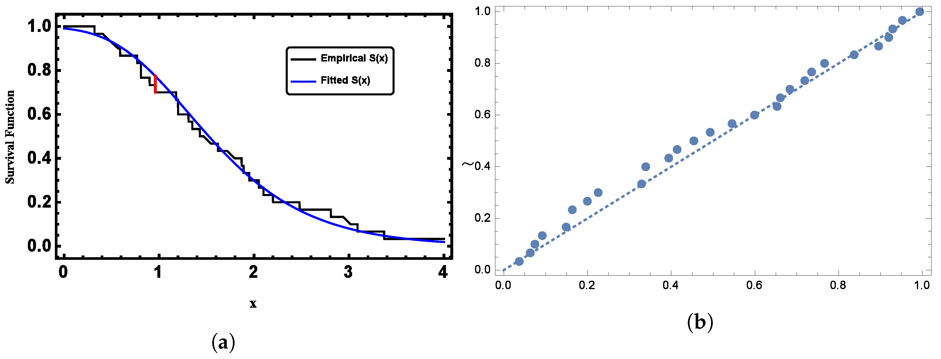
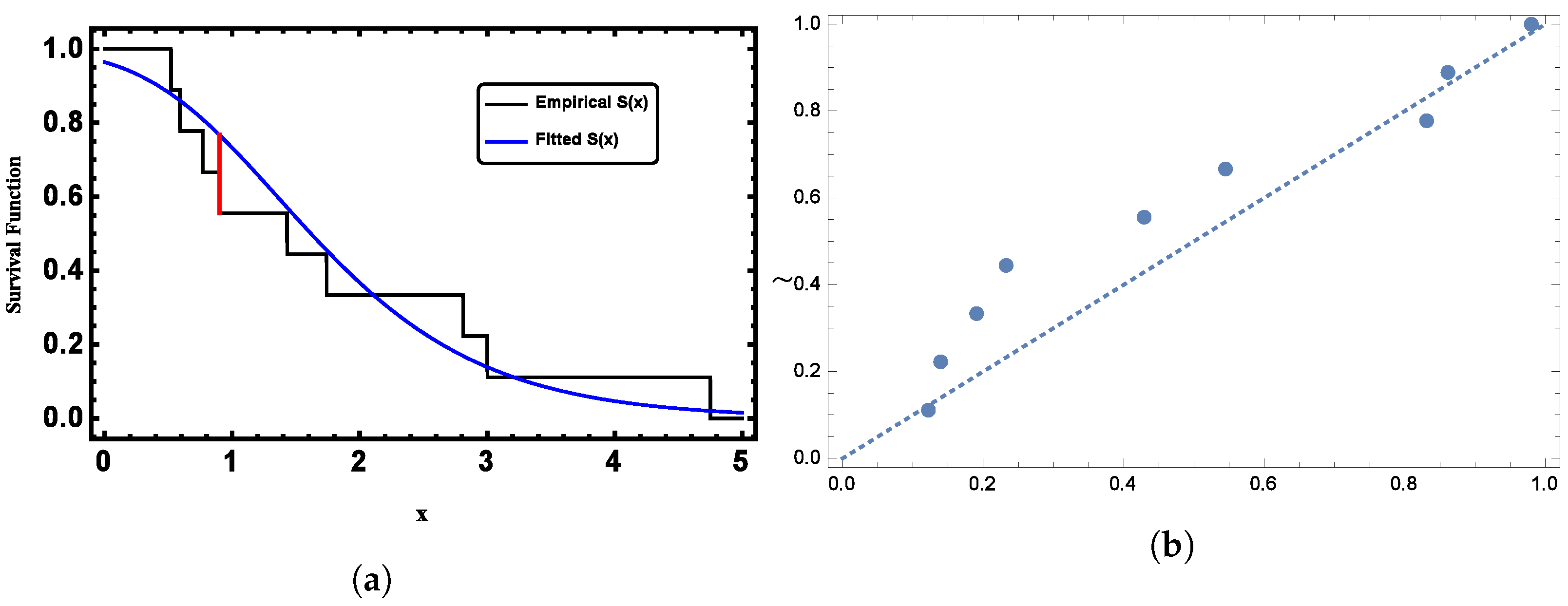
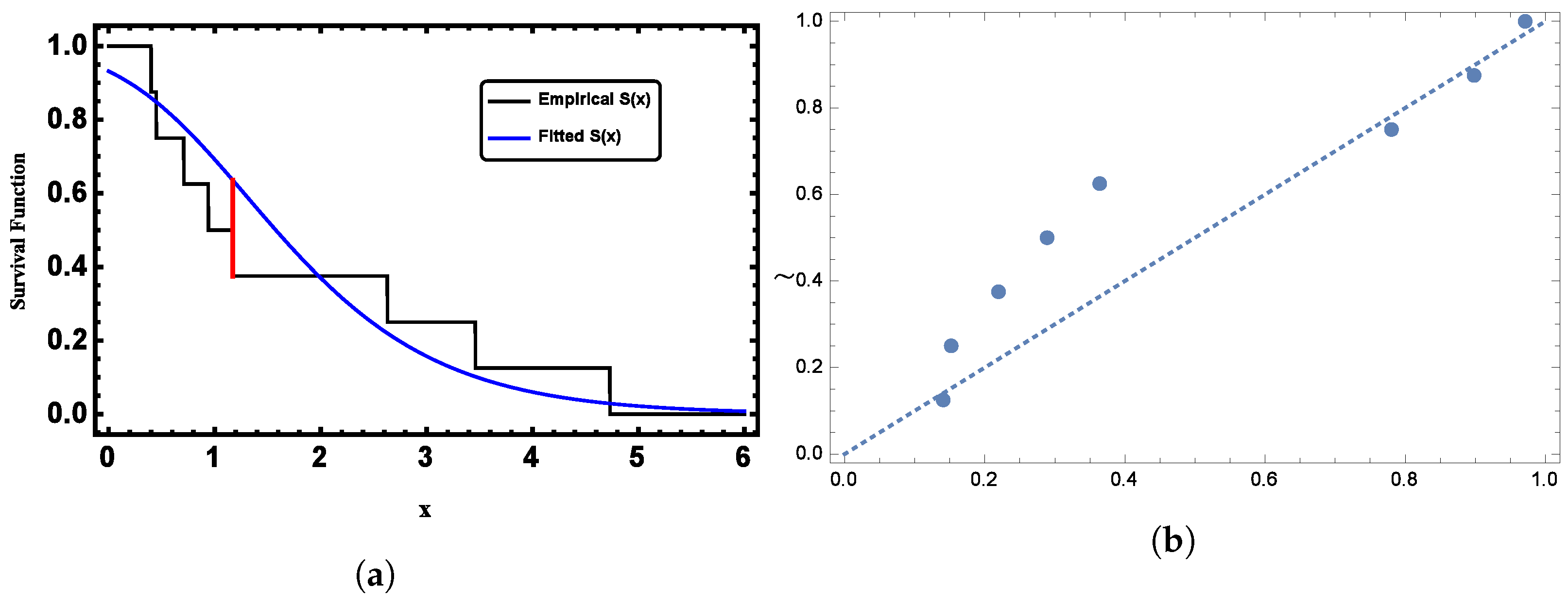
5. Application to Random Censored Data

In this section, we analyze two real datasets to illustrate the applicability of the GL distribution to censored data. The datasets and their corresponding fits are described as follows.

5.1. Dataset I

The first real dataset consisted of thirty consecutive values of March precipitation (in inches) recorded in Minneapolis/St. Paul, as reported by Hinkley [30]. The data points were as follows: $0.{77}^{*},1.{74}^{*},0.81,1.2,1.95,1.2,0.47,1.{43}^{*},3.37,2.2,3^{*},3.09,1.51,2.1,0.{52}^{*},1.62,1.31,$ $0.32,0.{59}^{*},0.81,2.{81}^{*},1.87,1.18,1.35,4.{75}^{*},2.48,0.96,1.89,0.9^{*},$ and $2.05.$ The censored observations are marked with asterisks.

The Kolmogorov–Smirnov (K-S) test was used to evaluate if the given data conformed to a GL distribution. The K-S statistic and its corresponding p-value were 0.0744 and 0.9918, respectively. This widely recognized measure of the goodness-of-fit suggests that the proposed model is appropriate for fitting the given censored data. Visually, as shown in Figure 6, it is evident that the GL distribution closely matched the pattern of the censored data.

For the censored observations $0.{77}^{*},1.{74}^{*},1.{43}^{*},3^{*},0.{52}^{*},0.{59}^{*},2.{81}^{*},4.{75}^{*},$ and $0.9^{*}$, we employed the K-S test to assess whether the data followed a GL distribution. The K-S test yielded a statistic of 0.2119, with a corresponding p-value of 0.7394. These results from this widely accepted goodness-of-fit measure indicate that the proposed GL model is suitable for fitting the given censored data. Figure 7 provides visual confirmation, clearly demonstrating that the GL distribution closely aligns with the pattern observed in the censored data.

Based on the dataset used in this study, we calculated estimates using MLEs for $\kappa =6.5$, $\alpha =2.0$, and $\psi =1.2$. These results are presented in

Table 1. Estimates for the censored Dataset I using classical and Bayesian methods.

Parameters	MLE		MCMC
	Mean	Length	SE	GE		Length
				$\mathit{\sigma }\mathbf{=}\mathbf{-}\mathbf{3}$	$\mathit{\sigma }\mathbf{=}\mathbf{3}$
$\kappa$	6.7388	4.3964	3.3807	3.5517	3.052	2.9426
$\psi$	1.2077	0.8179	1.4098	1.4514	1.3339	0.9597
$\alpha$	1.9703	2.9016	1.4441	1.2777	0.9546	1.1590

, along with the outcomes of the 95% ACIs. For Bayesian estimation, we used the MCMC method with a total of 12,000 samples. To ensure the stability of the estimation process, the first 2000 samples were discarded during the ’burn-in’ phase. Non-informative priors with hyperparameters set to $a_i=0$ for i from 1 to 6 were used to derive the Bayesian estimates for $\kappa$, $\psi$, and $\alpha$ under both the SE and GE loss functions. The Bayesian estimation results are comprehensively displayed in Table 1. Additionally, the 95% CRIs for $\kappa$, $\psi$, and $\alpha$ are detailed in Table 1.

5.2. Dataset II

The second dataset represented the time intervals between failures for a repairable item, as provided by Murthy et al. [31]. The dataset included the following values: $1.43,0.11,0.{71}^{*},0.77,2.{63}^{*},1.49,3.{46}^{*},2.46,0.59,0.74,1.23,0.{94}^{*},4.36,0.{40}^{*},1.74,4.{73}^{*},2.23,$ $0.{45}^{*},0.70,1.06,1.46,0.30,1.82,2.37,0.63,1.23,1.24,1.97,1.86,$ and $1.{17}^{*}.$ The censored observations are marked with asterisks. The K-S test was conducted to assess whether the data followed a GL distribution. The K-S statistic was 0.1104, with a corresponding p-value of 0.8192. This well-established measure of the goodness-of-fit indicated that the proposed model is suitable for the censored data. As illustrated in Figure 8, the GL distribution fit the pattern observed in the censored data very closely.

For the set of censored observations $0.{71}^{*},2.{63}^{*},3.{46}^{*},0.{94}^{*},0.{40}^{*},4.{73}^{*},0.{45}^{*},$ and $1.{17}^{*}$, we applied the K-S test to evaluate the data’s conformity to a GL distribution. The K-S test produced a statistic of 0.2610 accompanied by a p-value of 0.5613. These results from this widely accepted goodness-of-fit measure suggest that the proposed GL model is appropriate for the given censored data. Visual confirmation is provided in Figure 9, which clearly demonstrates that the GL distribution closely aligned with the pattern exhibited by the censored observations.

Using Dataset II, we computed estimates via MLEs for $\kappa =6.0$, $\alpha =1.5$, and $\psi =0.9$. These results are displayed in

Table 2. Estimates for the censored Dataset II using classical and Bayesian methods.

Parameters	MLE		MCMC
	Mean	Length	SE	GE		Length
				$\mathit{\sigma }\mathbf{=}\mathbf{-}\mathbf{3}$	$\mathit{\sigma }\mathbf{=}\mathbf{3}$
$\kappa$	5.6053	3.4173	3.1897	3.3337	2.9106	2.6732
$\psi$	1.2749	0.9024	1.2943	1.3288	1.2303	0.8077
$\alpha$	1.8565	2.7112	1.0529	1.1514	0.8706	1.2587

, and the corresponding 95% ACIs are provided in the same table. For Bayesian estimation, we employed the MCMC method, generating a total of 12,000 samples. To ensure the stability of the estimation process, the first 2000 samples were discarded during the burn-in phase. Non-informative priors with hyperparameters set to $a_i=0$ for $i=1$ to 6 were used to obtain Bayesian estimates for $\kappa$, $\psi$, and $\alpha$ under both the SE and GE loss functions. The Bayesian estimation results are comprehensively presented in Table 2. Additionally, the 95% CRIs for $\kappa$, $\psi$, and $\alpha$ are detailed in the same table.

6. Simulation Study

As shown in this section, a Monte Carlo simulation study was performed to assess the effectiveness and performance of various estimation techniques. We generated a randomly censored sample from the GL distribution using an algorithm. For the simulation, the parameters were set as $\kappa =3.5$, $\psi =2.5$, and $\alpha =1.5$. Maximum likelihood estimates for $\kappa$, $\psi$, and $\alpha$ were computed along with the ARB for different sample sizes. In the Bayesian analysis, we employed a gamma prior for all parameters, setting the hyper-parameters of the prior distribution as $a_1=a_3=a_5=3.5$ and $a_2=a_4=a_6=2.7$. The Bayesian estimates of the parameters were obtained under the SE and GE loss functions using the MCMC method. From a long chain of length, 10,000 were generated by the M-H algorithm, and the first 1000 values were discarded to eliminate the influence of initial parameter values.

The ARB was calculated using the following formula:

$$\mathrm{ARB}\left(\widehat{\varphi }\right)={\displaystyle \frac{\left|\frac{{\sum }_{i=1}^{1000}{\widehat{\varphi }}_i}{1000}-\varphi \right|}{\varphi }},\mathrm{where}i=1,2,3,\mathrm{and}({\varphi }_1,{\varphi }_2,{\varphi }_3)=(\kappa ,\psi ,\alpha ).$$

(28)

The classical and Bayesian estimates for the parameters $\kappa$, $\psi$, and $\alpha$, along with the corresponding ARB values, are discussed in

Table 3. Classical and Bayesian estimates for the parameter $\psi$, with the corresponding ARB values in parentheses.

n	MLE		MCMC
	Mean	Length	SE	GE		Length
				$\mathit{\sigma }\mathbf{=}\mathbf{-}\mathbf{3}$	$\mathit{\sigma }\mathbf{=}\mathbf{3}$
30	2.1608	1.4883	1.6984	1.7413	1.621	1.3497
	(0.7357)		(0.3206)	(0.3035)	(0.3516)
35	2.4911	1.347	2.1529	2.1970	2.0706	1.2092
	(0.6036)		(0.2688)	(0.2212)	(0.2718)
45	2.6678	1.3204	1.8509	1.8816	1.7932	0.9275
	(0.5671)		(0.2597)	(0.2474)	(0.2466)
55	2.4055	1.0928	1.9053	1.9311	1.8551	0.8669
	(0.5078)		(0.2379)	(0.2276)	(0.2579)
65	2.622	1.0621	2.0253	2.0500	1.9779	0.8688
	(0.4488)		(0.2199)	(0.2191)	(0.2089)
75	2.7086	1.0765	2.0835	2.1046	2.0429	0.8155
	(0.4235)		(0.2066)	(0.2081)	(0.2028)
85	2.5626	0.9429	2.1141	2.1351	2.0741	0.8076
	(0.4151)		(0.2043)	(0.2059)	(0.2004)
95	2.7228	0.9294	2.1670	2.1851	2.132	0.7695
	(0.4091)		(0.1932)	(0.1926)	(0.1972)
105	2.4087	0.7825	1.8364	1.8502	1.8093	0.6276
	(0.3365)		(0.1654)	(0.1599)	(0.1763)
115	2.6026	0.7167	2.0464	2.0606	2.0189	0.6132
	(0.3111)		(0.1514)	(0.1458)	(0.1425)

,

Table 4. Classical and Bayesian estimates for the parameter $\kappa$, with the corresponding ARB values in parentheses.

n	MLE		MCMC
	Mean	Length	SE	GE		Length
				$\mathit{\sigma }\mathbf{=}\mathbf{-}\mathbf{3}$	$\mathit{\sigma }\mathbf{=}\mathbf{3}$
30	3.6186	2.5604	2.2174	2.2845	2.0805	1.7035
	(0.8339)		(0.3665)	(0.3473)	(0.4056)
35	4.2924	2.4981	2.5072	2.5777	2.3653	1.6407
	(0.7264)		(0.2836)	(0.2635)	(0.3242)
45	3.1662	1.6388	1.9893	2.0306	1.9065	1.1317
	(0.6954)		(0.2316)	(0.2198)	(0.2553)
55	3.5482	1.6268	2.3282	2.3699	2.2435	1.1218
	(0.5138)		(0.2248)	(0.2129)	(0.2290)
65	3.3718	1.4416	2.2436	2.2763	2.1780	1.0605
	(0.4266)		(0.2159)	(0.2096)	(0.2077)
75	4.0464	1.3465	2.4913	2.5247	2.4241	1.0328
	(0.3561)		(0.2082)	(0.2087)	(0.2074)
85	3.7482	1.3281	2.4507	2.4802	2.3911	1.0109
	(0.3409)		(0.2028)	(0.2014)	(0.2018)
95	3.5422	1.2378	2.3801	2.4051	2.3303	0.9581
	(0.3121)		(0.1932)	(0.1828)	(0.1912)
105	3.3041	1.1063	2.2305	2.2515	2.1883	0.8396
	(0.3056)		(0.1627)	(0.1567)	(0.1608)
115	3.6497	1.0549	2.3962	2.4174	2.3537	0.8208
	(0.1528)		(0.1540)	(0.1493)	(0.1475)

and

Table 5. Classical and Bayesian estimates for the parameter $\alpha$, with the corresponding ARB values in parentheses.

n	MLE		MCMC
	Mean	Length	SE	GE		Length
				$\mathit{\sigma }\mathbf{=}\mathbf{-}\mathbf{3}$	$\mathit{\sigma }\mathbf{=}\mathbf{3}$
30	1.1860	1.7966	0.7858	0.8634	0.6473	0.9941
	(0.5093)		(0.4762)	(0.4244)	(0.4085)
35	1.2735	1.7000	0.8466	0.9221	0.7126	0.9855
	(0.4951)		(0.4356)	(0.3853)	(0.4249)
45	1.1590	1.3621	0.6437	0.6864	0.5634	0.6468
	(0.4273)		(0.3708)	(0.3424)	(0.3244)
55	1.1035	1.1560	0.6959	0.7345	0.6242	0.6296
	(0.3644)		(0.3361)	(0.3103)	(0.3039)
65	1.0371	1.0073	0.6347	0.6655	0.5761	0.5413
	(0.3386)		(0.3069)	(0.3064)	(0.3015)
75	1.6173	1.0049	0.7967	0.8276	0.7383	0.5126
	(0.3282)		(0.2988)	(0.2483)	(0.2478)
85	1.1491	0.9650	0.7025	0.7278	0.6536	0.5252
	(0.2339)		(0.2617)	(0.2348)	(0.2343)
95	1.0893	0.8689	0.6548	0.6762	0.6134	0.4626
	(0.2138)		(0.2135)	(0.2092)	(0.2011)
105	1.0506	0.7989	0.6083	0.6267	0.5730	0.4116
	(0.1996)		(0.1944)	(0.1822)	(0.1810)
115	1.1886	0.6625	0.6745	0.6926	0.6395	0.4096
	(0.1476)		(0.1303)	(0.1383)	(0.1237)

.

Based on the results of the simulation study, we conclude that

• The ARB decreases as the sample size increases.
• The ARB is lower in the Bayesian approach compared to the classical approach, indicating that the MCMC method performs better than MLE.
• It was observed that the length of the ACI was greater than that of the Bayesian intervals.
• The ARB was lower in the Bayesian approach under the GE loss function compared to the SE loss function, suggesting that the GE method outperforms the SE method.

7. Concluding Remarks

In conclusion, we explored both the interval and point estimates of the parameters, focusing on classical methods, particularly MLE. We derived ACIs for the parameters using MLE and examined Bayesian estimators with informative priors for both the SE and GE loss functions. To compare the performance of classical and Bayesian estimators, we conducted a comprehensive computational analysis through a Monte Carlo simulation study. The findings indicate that the Bayesian intervals tend to be shorter than the classical ACI lengths, suggesting a potential advantage in using Bayesian methods for parameter estimation.

Looking ahead, future research should aim to enhance these methodologies further, exploring additional estimation techniques and their applications in various contexts. This could lead to improved accuracy and reliability in parameter estimation for the generalized logistic distribution under random censoring scenarios.

References

1. Gilbert, J.P. Random Censorship. Ph.D. Thesis, University of Chicago, Chicago, IL, USA, 1962. [Google Scholar]
2. Breslow, N.; Crowley, J. A large sample study of the life table and product limit estimates under random censorship. Ann. Stat. 1974, 2, 437–453. [Google Scholar] [CrossRef]
3. Koziol, J.; Green, S. A Cramer–von Mises statistic for randomly censored data. Biometrika 1976, 633, 465–474. [Google Scholar] [CrossRef]
4. Ghitany, M.E.; Al-Awadhi, S. Maximum likelihood estimation of Burr XII distribution parameters under random censoring. J. App. Stat. 2002, 29, 955–965. [Google Scholar] [CrossRef]
5. Liang, T. Empirical Bayes testing for uniform distributions with random censoring. J. Stat. Theory Pract. 2008, 2, 633–649. [Google Scholar] [CrossRef]
6. Saleem, M.; Aslam, M. On Bayesian analysis of the Rayleigh survival time assuming the random censor time. Pak. J. Stat. 2009, 25, 71–82. [Google Scholar]
7. Danish, M.Y.; Aslam, M. Bayesian inference for the randomly censored Weibull distribution. J. Stat. Comput. Simul. 2014, 84, 215–230. [Google Scholar] [CrossRef]
8. Vivekanand, H.K.; Kumar, K. Estimation in Maxwell distribution with randomly censored data. J. Stat. Comput. Simul. 2015, 85, 3560–3578. [Google Scholar]
9. Garg, R.; Dube, M.; Kumar, K.; Krishna, H. On randomly censored generalized inverted exponential distribution. Am. J. Math. Manag. Sci. 2016, 35, 361–379. [Google Scholar] [CrossRef]
10. Krishna, H.; Goel, N. Maximum likelihood and Bayes estimation in randomly censored geometric distribution. J. Probab. Stat. 2017, 2017, 4860167. [Google Scholar] [CrossRef]
11. Krishna, H.; Goel, N. Classical and Bayesian inference in two parameter exponential distribution with randomly censored data. Comput. Stat. 2018, 33, 249–275. [Google Scholar] [CrossRef]
12. Kumar, K.; Kumar, I. Estimation in inverse Weibull distribution based on randomly censored data. Statistica 2019, 79, 47–74. [Google Scholar]
13. Garg, R.; Dube, M.; Krishna, H. Estimation of parameters and reliability characteristics in Lindley distribution using randomly censored data. Stat. Opt. Inform. Comput. 2020, 8, 80–97. [Google Scholar] [CrossRef]
14. Ajmal, M.; Danish, M.Y.; Arshad, I.A. Objective Bayesian analysis for Weibull distribution with application to random censorship model. J. Stats. Comput. Simul. 2022, 92, 43–59. [Google Scholar] [CrossRef]
15. Goel, N.; Krishna, H. Different methods of estimation in two parameter Geometric distribution with randomly censored data. Int. J. Syst. Assur. Eng. Manag. 2022, 13, 1652–1665. [Google Scholar] [CrossRef]
16. Hasaballah, M.M.; Al-Babtain, A.A.; Hossain, M.M.; Bakr, M.E. Theoretical Aspects for Bayesian Predictions Based on Three-Parameter Burr-XII Distribution and Its Applications in Climatic Data. Symmetry 2023, 15, 1552. [Google Scholar] [CrossRef]
17. Hasaballah, M.M.; Tashkandy, Y.A.; Balogun, O.S.; Bakr, M.E. Bayesian inference for the inverse Weibull distribution based on symmetric and asymmetric balanced loss functions with application. Eksploat. Niezawodn. Maint. Reliab. 2024, 26, 187158. [Google Scholar] [CrossRef]
18. Hasaballah, M.M.; Tashkandy, Y.A.; Balogun, O.S.; Bakr, M.E. Statistical inference of unified hybrid censoring scheme for generalized inverted exponential distribution with application to COVID-19 data. AIP Adv. 2024, 14, 045111. [Google Scholar] [CrossRef]
19. Hasaballah, M.M.; Balogun, O.S.; Bakr, M.E. Point and interval estimation based on joint progressive censoring data from two Rayleigh-Weibull distribution with applications. Phys. Scr. 2024, 99, 8. [Google Scholar] [CrossRef]
20. Balakrishnan, N.; Leung, M.Y. Order statistics from the type I generalized logistic distribution. Commun. Stat. Simul. Comput. 1988, 17, 25–50. [Google Scholar] [CrossRef]
21. Balakrishnan, N. Handbook of the Logistic Distribution, 2nd ed.; Marcel Dekker: New York, NY, USA, 2010; pp. 50–77. [Google Scholar]
22. Gupta, R.D.; Kundu, D. Generalized logistic distributions. J. Appl. Stat. Sci. 2010, 18, 51–66. [Google Scholar]
23. Alkasasbeh, M.R.; Raqab, M.Z. Estimation of the generalized logistic distribution parameters: Comparative study. Stat. Methodol. 2009, 6, 262–279. [Google Scholar] [CrossRef]
24. Asgharzadeh, A. Point and interval estimation for a generalized logistic distribution under progressive type-II censoring. Commun. Stat. Theory Methods 2006, 35, 1685–1702. [Google Scholar] [CrossRef]
25. Johnson, N.L.; Kotz, S.; Balakrishnan, N. Continuous Univariate Distributions, 2nd ed.; Wiley and Sons: New York, NY, USA, 1995; Volume 2. [Google Scholar]
26. Li, M.; Yan, L.; Qiao, Y.; Cai, X.; Said, K.K. Generalized Fiducial Inference for the Stress–Strength Reliability of Generalized Logistic Distribution. Symmetry 2023, 15, 1365. [Google Scholar] [CrossRef]
27. Asgharzadeh, A.; Valiollahi, R.; Raqab, M.Z. Estimation of the stress–strength reliability for the generalized logistic distribution. Stat. Methodol. 2013, 15, 73–94. [Google Scholar] [CrossRef]
28. Metropolis, N.; Rosenbluth, A.W.; Rosenbluth, M.N.; Teller, A.H.; Teller, E. Equations of state calculations by fast computing machines. J. Chem. Phys. 1953, 21, 1087–1091. [Google Scholar] [CrossRef]
29. Neal, R.M. Slice sampling. Ann. Stat. 2003, 31, 705–767. [Google Scholar] [CrossRef]
30. Hinkley, D. On quick choice of power transformations. Appl. Stat. 1977, 26, 67–69. [Google Scholar] [CrossRef]
31. Murthy, D.N.P.; Xie, M.; Jiang, R. Weibull models. In Wiley Series in Probability and Statistics; Wiley: Hoboken, NJ, USA, 2004. [Google Scholar]
Figure 1. Density plot of the GL distribution for different values of κ , with ψ = 1 .
Symmetry 16 01240 g001
Figure 2. Density plot of the GL distribution for different values of κ , with ψ > 1 .
Symmetry 16 01240 g002
Figure 3. Density plot of the GL distribution for different values of κ , with ψ < 1 .
Symmetry 16 01240 g003
Figure 4. Illustration of the CDF of the GL distribution for various values of κ , with ψ as constant.
Symmetry 16 01240 g004
Figure 5. (a) The hazard rate function of the GL distribution for different values of κ . (b) The survival plots of the GL distribution for various values of κ .
Symmetry 16 01240 g005
Figure 6. (a) Plots of the fitted function compared to the empirical CDF for Dataset I. and (b) Plots of the PP plot for Dataset I.
Symmetry 16 01240 g006
Figure 7. (a) Plots of the fitted function compared to the empirical CDF for the censored observations from Dataset I. and (b) Plots of the PP plot for the censored observations from Dataset I.
Symmetry 16 01240 g007
Figure 8. (a) Plots of the fitted function compared to the empirical CDF for Dataset II. and (b) Plots of the PP plot for Dataset II.
Symmetry 16 01240 g008
Figure 9. (a) Plots of the fitted function compared to the empirical CDF for the censored observations from Dataset II. and (b) Plots of the PP plot for the censored observations from Dataset II.
Symmetry 16 01240 g009