Abstract
This paper aims to adapt and apply genetic distance metrics in biomedical signal processing to improve the classification and monitoring of neurological disorders, specifically Alzheimer’s disease and frontotemporal dementia. The primary objectives are: (1) to quantify the variability in EEG signal patterns among the distinct subtypes of neurodegenerative disorders and healthy individuals, and (2) to explore the potential of a novel genetic similarity metric in establishing correlations between brain signal dynamics and clinical progression. Using a dataset of resting-state EEG recordings (eyes closed) from 88 subjects (36 with Alzheimer’s disease, 23 with frontotemporal dementia, and 29 healthy individuals), a comparative analysis of brain activity patterns was conducted. Symmetry plays a critical role in the proposed genetic similarity metric, as it captures the balanced relationships between intra- and inter-group EEG signal patterns. Our findings demonstrate that this approach significantly improves disease subtype identification and highlights the potential of the genetic similarity metric to optimize the predictive models. Furthermore, this methodology supports the development of personalized therapeutic interventions tailored to individual patient profiles, making a novel contribution to the field of neurological signal analysis and advancing the application of EEG in personalized medicine.
1. Introduction
Neurological disorders, such as Alzheimer’s disease and dementia, exhibit significant variability in clinical presentation and progression. Factors such as the age of onset, rate of cognitive decline, and treatment response differ widely among patients, making it crucial to understand and quantify this variability to develop personalized treatments and predict disease progression.
Biomedical signal processing techniques, such as electroencephalography (EEG), can reveal the variability in brain activity patterns among patients with Alzheimer’s disease and dementia. These variations often correlate with symptom severity and disease progression. By analyzing brain signals, it becomes possible to identify the subtypes of these disorders, facilitating personalized treatment strategies. However, variability can complicate the early and accurate diagnosis of Alzheimer’s disease and dementia. It may lead to the misdiagnosis or delayed identification of the disease. Conversely, quantifying variability could enable the personalization of treatments. For instance, by identifying the different subtypes of the disease, it becomes possible to tailor the responses to specific therapies, illustrating how the genetic distance and variability in brain signals can inform the treatment choices.
Personalized medicine, as described by [1], involves tailoring medical treatments based on an individual’s genetic information to predict their response to therapies and select the most effective options. Similarly, the National Research Council [2] defines personalized medicine, or precision medicine, as an approach that incorporates the individual variations in genes, environment, and lifestyle to improve prevention, diagnosis, and treatment. This personalized strategy enhances the therapeutic efficacy, minimizes side effects by avoiding unsuitable treatments, and optimizes resource allocation. It has expanded to include not only genetic data but also biomarkers, lifestyle, and environmental factors, finding significant applications in fields like oncology, where the therapies target specific genetic mutations, and cardiology, where treatments account for genetic and physiological factors.
The concept of genetic distance, originally proposed for algorithm selection in the Asymmetric Travelling Salesman Problem (ATSP) [3], has been adapted to biomedical signal processing to quantify the variability in patient data, particularly in neurological disorders like Alzheimer’s disease and dementia. In this context, the genetic distance quantifies the similarity or difference between physiological signals, such as electroencephalograms (EEGs) or electrocardiograms (ECGs), across individuals or within the same individual over time. This metric reflects the signal divergence or similarity, enabling the identification of patterns indicative of pathological conditions, disease progression, or treatment response.
The term “genetic” is attributed to the quantification of molecular markers; for example, in a jungle, a lion and a leopard exhibit similar characteristics, but some differences are reflected in their genes. Similarly, the genetic distance in biomedical signals reflects how similar or divergent these signals are, enabling the identification of patterns that may be indicative of a pathological condition, its progression, or response to treatment.
For instance, in patients with neurological disorders such as Alzheimer’s disease or dementia, the genetic distance can be utilized to assess the differences in brain activity, aiding in the distinction between disease subtypes, predicting disease progression, and personalizing therapeutic interventions. This metric is obtained by analyzing the frequency and distribution of the specific features of biomedical signals, where similarity is observed when shared features have a frequency greater than a certain threshold.
This paper explores the use of EEG analysis as an accessible and cost-effective alternative to genetic testing for personalizing treatments in neurological disorders. By identifying the patterns in EEG signals, the study aims to classify the disease subtypes, monitor progression, and support early intervention, particularly in resource-limited settings. Furthermore, it evaluates the effectiveness and accessibility of this approach compared to traditional genetic methods, focusing on its potential to broaden the reach of personalized medicine.
The use of biomedical signals, such as electroencephalograms (EEGs) and electrocardiograms (ECGs), offers a more accessible and cost-effective alternative to genetic testing, which can be prohibitively expensive [4]. Many medical facilities already possess the necessary equipment to capture these signals, eliminating the need for new technological investments. Furthermore, this approach enables more patients, particularly in resource-limited settings, to access personalized treatments, facilitating its implementation in various regions of the world and promoting greater equity in healthcare [2].
The analysis of biomedical signals, such as EEG, presents a viable alternative for the early detection and continuous monitoring of neurological disorders such as Alzheimer’s disease [5]. By identifying the specific patterns in these signals, it is possible to personalize treatments effectively, tailoring them to the individual patient’s needs without relying on costly genetic analysis [6]. This approach not only facilitates early intervention but also allows for the accurate tracking of disease progression, thereby optimizing treatment [7].
The rising incidence of neurological disorders, including Alzheimer’s disease and dementia, calls for novel strategies to comprehend and address these intricate conditions. The recent progress in biomedical signal processing has created fresh opportunities for the analysis of physiological data, allowing researchers to measure the variability in patient responses. This paper suggests that the notion of genetic distance, which has been conventionally employed in genetics to evaluate the similarities or differences between organisms, can be suitably modified to examine the variability in physiological signals among individuals suffering from neurological disorders.
Symmetry is a key principle across various scientific fields, symbolizing balance, proportion, and structure within complex systems. In neurological signal processing, it plays a crucial role in examining the balance or imbalance in brain activity patterns among healthy individuals and those affected by neurodegenerative conditions. This research utilizes symmetry by introducing a genetic distance metric that harmonizes intra- and inter-group differences, enabling a more refined classification of disease subtypes. Genetic distance, in its traditional form, measures the divergence in genetic markers, such as SNPs or microsatellites, across populations or individuals. We have adapted this concept to biomedical signal processing by redefining the genetic distance as a quantitative measure of the differences in signal patterns. Specifically, our metric evaluates the variability in features like frequency, amplitude, and phase, which may reflect the genetic, environmental, or pathological influences. Unlike traditional genetic distances based solely on genetic markers, our metric incorporates the dynamic and temporal characteristics of EEG signals, making it uniquely suited for applications in neurological disorders. This redefinition bridges genetic variability with physiological signal analysis, allowing for subtle changes in brain activity to be quantified and linked to disease progression or treatment responses.
2. Theoretical Foundations
2.1. Genetic Distance
The genetic distance is a quantitative measure used to assess the similarity or divergence between individuals, populations, or genetic markers, such as SNPs, insertions, deletions, and microsatellites. In biomedical signal processing, this concept is adapted to quantify the differences in signal patterns, such as EEG, between individuals or over time.
In biomedical signals, the genetic distance quantifies the similarity or divergence in patterns based on features such as frequency, amplitude, and phase, which reflect genetic, environmental, or pathological influences. This metric is crucial for identifying and classifying the patterns associated with medical conditions, enabling the detection of subtle changes indicative of disease progression or treatment response.
Common distance metrics in biomedical signal analysis include the following:
- Modified Euclidean Distance: incorporates weights for features, allowing adjustments based on their importance [8].
- Mahalanobis Distance: accounts for correlations between variables, which is useful for multivariate datasets [9].
- Entropy-based Distance: quantifies the divergence between probability distributions using Shannon entropy [10].
While effective in specific contexts, these metrics may fail to capture the dynamic and non-linear variability present in biomedical signals.
Genetic distances can be categorized into two main groups:
- Geometric Distances: these measure similarity based on the allele frequencies across genetic systems, often visualized geometrically as distances between points on a hypersphere. Examples include chord distance [11] and Rogers distance [12].
- Evolutionary Model-based Distances: These account for the variation caused by mutation and genetic drift, assuming that the markers are not influenced by natural selection. Distances based on the infinite allele model treat each mutation as creating a new allele, making all allelic states equally related.
The proposed genetic similarity metric was compared with commonly used distance metrics (Table 1) to demonstrate its advantages in EEG-based neurological disorder analysis. This comparison highlights the strengths and limitations of each method, emphasizing how our approach captures signal variability and provides clinically relevant insights.

Table 1.
Strengths and limitations of distance metrics in biomedical signal analysis.
Genetic distances reflect the biological variation influenced by factors such as genetic flow, drift, and geographic distribution [13,14]. Genetic distances do not always correlate with physical or geographic barriers, as observed in populations with significant genetic divergence despite proximity [15,16].
In genetic studies, similar profiles may result from homoplasy (evolutionary convergence) rather than direct relationships, an idea adapted here for signal analysis to interpret the variability in physiological patterns [17,18].
2.2. Relevant Characteristics of Biomedical Signals
Feature extraction involves analyzing biomedical signals, to decompose the complex signal into simpler, quantifiable components. The important features are as follows:
- Frequency bands. Specific intervals within the EEG frequency spectrum, such as Delta (0.5–4 Hz), Theta (4–8 Hz), Alpha (8–13 Hz), Beta (13–30 Hz), and Gamma (>30 Hz) [19]. Analyzing the power distribution in these bands provides insights into brain states and cognitive processes, offering crucial features for neurological analysis.
- Entropy. A measure of signal complexity or variability, used in EEG analysis to differentiate between chaotic and organized patterns, providing insights into neural dynamics [20].
- Dominant Frequency. The frequency with the highest amplitude in a signal, indicative of specific cognitive or pathological states, serving as a key feature in brain activity assessment [21].
- Other Metrics. Amplitude variance, peak duration, and zero-crossing rate offer additional insights into signal dynamics, complementing frequency and entropy analyses [22,23].
2.3. Biomedical Signal Processing Techniques Relevant to the Study
Biomedical signal processing plays a critical role in the early diagnosis and monitoring of neurodegenerative diseases like Alzheimer’s and dementia, enabling the analysis and identification of anomalous brain activity patterns indicative of these conditions [24].
Techniques like EEG, MRI, PET, voice analysis, evoked potential signals, and heart rate variability (HRV) are widely used for studying Alzheimer’s and other dementias [19]. The integration of these methods enhances early diagnosis and monitoring, enabling timely interventions and personalized treatments.
- Electroencephalography (EEG). Biomedical signal processing plays a critical role in the early diagnosis and monitoring of neurodegenerative diseases like Alzheimer’s and dementia, enabling the analysis and identification of anomalous brain activity patterns indicative of these conditions [24].
- Magnetic Resonance Imaging (MRI). Produces detailed brain images to identify structural changes like hippocampal atrophy, commonly observed in Alzheimer’s. It supports hippocampal volumetry and functional connectivity analysis.
- Positron Emission Tomography (PET). Measures glucose metabolism and detects abnormal protein deposits (beta-amyloid, tau) to differentiate Alzheimer’s from other dementias.
- Evoked Potential Signal Analysis. Evaluates the brain responses to stimuli, revealing cognitive impairments and aiding in the early detection of mild cognitive impairment (MCI).
- Heart Rate Variability (HRV) Analysis. Monitors autonomic dysfunction and its link to dementia progression by analyzing the variability in heartbeat intervals.
- Voice and Language Analysis. Detects cognitive decline through changes in speech patterns, including verbal coherence and language complexity, offering a non-invasive diagnostic tool.
- Machine Learning and Deep Learning techniques. Process biomedical data to classify brain images and predict disease progression, leveraging patterns in EEG and fMRI data.
2.4. Relationship Between Genetic Variability and Patterns in Brain Signals
Biomedical signals enable early diagnosis, disease monitoring, and cognitive function assessment. The key applications include identifying the early signs of disease, evaluating the treatment effectiveness, and understanding the impact of neurodegenerative disorders on cognitive processes [25,26,27].
The genetic studies of Alzheimer’s disease (AD) highlight a network of genes involved in the immune response, metabolism, and neurodegeneration [28]. Familial AD is linked to mutations in PSEN1, PSEN2, and APP, while sporadic AD, primarily affecting individuals over 65, is associated with genetic variants like the APOE ε4 allele [29,30,31].
The United Kingdom Biobank [32] identified brain networks vulnerable to ageing, Alzheimer’s, and modifiable risk factors like diabetes and air pollution, underscoring their role in brain frailty beyond age and sex.
One study found that genetic variants primarily influence cognitive development, being associated with increased education and brain volume, but not dementia, suggesting that cognition has limited value as a biomarker of neurodegeneration [33]. The genetic variability in FOXP2 is linked to frontotemporal dementia (FTD), affecting the age of onset, cognitive abilities, and brain atrophy [34,35]. These findings suggest that FOXP2 regulatory pathways influence the brain areas impacted by dementia.
2.5. Subtypes of Alzheimer’s Disease
Alzheimer’s disease can be classified into several subtypes, each distinguished by specific characteristics, including progression rate, predominant symptoms, and pathological patterns. These classifications are primarily based on clinical and neuropathological research.
- Late-onset Alzheimer’s disease (LOAD). The most common form of Alzheimer’s disease, affecting individuals over 65 years of age. Understanding factors influencing LOAD progression is increasingly critical due to global ageing trends.
- Early-Onset Alzheimer’s Disease (EOAD). Occurs before the age of 65, representing 5–10% of cases. EOAD progresses more aggressively due to a higher burden of tau and amyloid pathology [36,37,38,39].
- Atypical presentations of Alzheimer’s disease (AD). Include variants like primary progressive aphasia (PPA), posterior cortical atrophy (PCA), and corticobasal syndrome (CBS). These atypical forms require tailored diagnostic and management strategies due to distinct neuroanatomical and neuropsychological profiles [40,41,42].
- Alzheimer’s disease and vascular dementia (VaD). Frequently co-occurring, vascular factors such as hypertension and diabetes exacerbate Alzheimer’s progression. Research highlights the impact of vascular risk factors on cognitive decline [43,44,45,46].
- Familial Alzheimer’s disease (FAD). A genetically inherited form of Alzheimer’s disease, often presenting before 65, associated with mutations in APP, PSEN1, and PSEN2 genes [46,47,48,49,50]. Though rare (1–2% of cases), FAD provides critical insights into Alzheimer’s pathophysiology.
There are other subtypes:
- Neuroanatomical subtypes. Neuroanatomical subtypes, identified through MRI and PET imaging, highlight the distinct patterns of brain atrophy linked to clinical symptoms, enhancing the diagnostic accuracy and intervention planning [51].
- Clinical subtypes. Clinical subtypes, based on cognitive profiles, biomarkers, and imaging findings, offer a nuanced framework for understanding Alzheimer’s, as proposed by the Dubois criteria [52].
- Biomarker subtypes. Biomarker-based subtypes leverage the advancements in molecular imaging and fluid biomarkers to categorize Alzheimer’s, enhancing our understanding of its pathophysiology.
- Brain wave pattern subtypes. Subtypes identified through EEG analysis reveal the differences in brain wave patterns (Alpha, Beta, Theta, Delta), correlating with cognitive states and Alzheimer’s progression.
Alzheimer’s spectrum disorder (ASD) refers to the range of clinical and biological manifestations of Alzheimer’s disease, from mild cognitive impairment to advanced dementia. This spectrum is critical for understanding the disease progression and for the development of appropriate therapeutic interventions. Recent research has emphasized the importance of biomarkers and neuroimaging techniques in the identification and classification of the different stages of the disease:
- 5.
- The preclinical stage of Alzheimer’s disease (AD). The preclinical stage occurs before clinical symptoms manifest, marked by beta-amyloid and tau accumulation detectable via biomarkers and imaging.
- 6.
- Mild cognitive impairment (MCI). MCI represents an intermediate stage between normal ageing and dementia. Biomarkers like phosphorylated tau and imaging techniques such as PET provide accurate risk assessments for progression to dementia [53,54].
3. Methodology
The genetic distance metric introduced in this study integrates the concept of symmetry by assigning equal weight to the differences in EEG features, such as frequency band powers, across the participants. This methodology provides a balanced depiction of the variability both within and between clinical groups, improving the metric’s interpretability in analyzing neurological disorders.
Box 1 illustrates the methodological process designed to investigate the relationship between the genetic distance and patterns in brain signals, with a focus on personalizing the treatment for neurological disorders such as Alzheimer’s and dementia. The diagram details each of the key stages, from data collection and pre-processing to calculating the genetic distance, analyzing the variability, developing predictive models, and applying these results in the creation of personalized treatment plans.
Box 1. Pseudocode 1 methodological process.
1. Data Collection
a. Define the EEG dataset path.
b. Load participant metadata from a TSV file (participant_id, group).
c. Initialize the data structures to store results:
- Powers per frequency band.
- Basic signal statistics.
- Clustering results and statistical analysis.
2. Data Preprocessing
For each participant in the dataset:
a. Load the corresponding EEG file.
If the file does not exist:
- Log an error and continue to the next participant.
b. Filter the signal for the relevant frequencies (1–40 Hz).
c. Extract the raw data from the signal (form: channels x time).
d. Calculate the basic statistics for each channel:
- Mean.
- Standard deviation.
- Range.
e. Calculate the average powers per frequency band (Delta, Theta, Alpha, Beta) using Welch’s method.
f. Store the calculated statistics and powers in the corresponding data structures.
3. The Genetic Distance Matrix Calculation quantifies the degree of similarity or divergence in EEG signal patterns across participants. This is essential for clustering participants into subtypes, enabling the identification of distinct disease patterns and facilitating personalized treatment strategies. Additionally, the matrix supports the exploration of the relationships between EEG signal variability and clinical biomarkers, enhancing the clinical relevance of the proposed methodology.
a. Initialize an empty distance matrix of size n × n (n = number of participants).
b. Define the weights (wk) for each trait based on its biological relevance, informed by prior studies and domain-specific knowledge.
c. For each pair of participants (i, j):
-Calculate the adapted genetic distance:
- Where:
- D (i, j): adapted genetic distance between participants i and j.
- wk: weight assigned to feature k based on its biological relevance.
- xik and xjk: values of feature k for participants i and j.
- Store D (i, j) in the distance matrix.
c. Display the distance matrix as a heat map.
d. Save the distance matrix for further analysis.
4. Classification of Subtypes by Clustering
For each group of participants (Alzheimer’s, Dementia, Control):
a. Select the relevant characteristics (power and statistics).
b. Apply the K-Means algorithm to cluster into 3 subtypes.
c. Assign subtype labels to each participant.
d. Store the results in a file for further analysis.
5. Statistical Analysis
a. Perform ANOVA tests for each frequency band within each group:
- Compare the differences between the subtypes.
b. Record the statistics of the results (F and p-values).
6. Visualization and Generation of the Results
a. Create graphs to represent the results:
- Power distribution by subtype and group.
- Heat map of distances between the participants.
b. Generate a final report including:
- Overall summary of the analysis.
- Representative graphs.
- Clustering and ANOVA results.
c. Save all the results in accessible formats (CSV, images, PDF)
3.1. Data Collection
Brain signals are the electrical and chemical manifestations of neural activity, captured by using techniques such as electroencephalography (EEG), magnetoencephalography (MEG), or functional magnetic resonance imaging (fMRI). The patterns in these signals reflect the synchronous and asynchronous activity of neural networks.
In this research, we used a dataset containing resting-state EEG [55] recordings with eyes closed, collected from a total of 88 subjects. This dataset included 36 patients diagnosed with Alzheimer’s disease, 23 with frontotemporal dementia, and 29 healthy individuals, allowing for a comparative analysis of the brain activity patterns associated with different neurodegenerative conditions and subjects without pathologies. The data are publicly available and can be downloaded from the OpenNeuro repository hosted on GitHub, ensuring their accessibility for future studies and independent validation.
3.2. Data Preprocessing
In this phase, the preprocessing pipeline ensures the removal of artefacts and noise that could distort the biomedical signals, while preparing the data for analysis. The steps include signal cleaning, normalization, and the extraction of the relevant features for the subsequent analysis. Each step is outlined below to provide transparency and reproducibility.
- Artefact Removal. Non-neural artefacts, such as eye blinks, muscle noise, and electrical interference, were addressed using the established preprocessing techniques. Independent Component Analysis (ICA) and notch filters were applied to remove these artefacts effectively.
- Signal Filtering. The EEG signals were band-pass filtered to retain frequencies between 1 and 40 Hz, which are relevant for capturing the neural activity associated with cognitive and neurological processes. This step eliminates low-frequency drifts and high-frequency noise, ensuring that the signal contains meaningful neural activity.
- Raw Data Extraction. The filtered EEG data were extracted in a matrix format, where rows represented individual channels (electrodes) and columns represented time samples. This structure allowed for channel-specific analysis across the entire signal duration.
- Feature Extraction. Several features were computed from the preprocessed EEG data to characterize the signal for subsequent analysis:
- (a)
- Power in Specific Frequency Bands: The average power within Delta (1–4 Hz), Theta (4–8 Hz), Alpha (8–12 Hz), and Beta (13–30 Hz) bands was calculated using Welch’s method. This method estimates the power spectral density by segmenting the signal into overlapping windows and applying a smoothing function.
- (b)
- Basic Signal Statistics: for each channel, we computed the mean, standard deviation, and range to summarize the overall signal variability and amplitude characteristics.
- (c)
- Entropy: Shannon entropy was computed to quantify the signal complexity and predictability.
- (d)
- Dominant Frequency: the frequency with the highest power within the spectrum was identified as the dominant frequency for each channel.
- Normalization. Each extracted feature (power in frequency bands, entropy, dominant frequency) was normalized to ensure that all the features contributed equally to the subsequent genetic distance calculation. This step balanced the impact of features with different scales or magnitudes.
- Multidimensional Representation. The extracted features were organized into a multidimensional space, where each dimension corresponded to a specific signal feature. Each participant’s EEG data were represented as a point in this space, facilitating the computation of genetic distances between signals.
- Data Storage. The processed data, including feature matrices and computed statistics, were stored in structured formats for integration with the genetic distance metric and subsequent clustering analysis.
3.3. Genetic Distance Calculation
The genetic distance is a quantitative measure of the similarity or difference between the genomes of different individuals or populations. In this study, the genetic distance was adapted for biomedical signal processing, specifically to quantify the variability in EEG patterns associated with neurological disorders. By calculating the genetic distance between each pair of participants, the method allows for the identification of the subtle variations in signal features such as frequency, amplitude, and phase. These variations are critical for distinguishing between the subtypes of neurodegenerative diseases, such as Alzheimer’s disease and frontotemporal dementia, and for understanding intra- and inter-group relationships.
The adapted genetic distance is calculated as follows (Equation (1)):
- -
- D (i, j) represents the genetic distance between participants i and j.
- -
- wk is the weight assigned to feature k based on its biological relevance.
- -
- xik and xjk are the values of feature k for participants i and j.
The features selected for this calculation include the following:
- -
- Frequency band powers: Delta (0.5–4 Hz), Theta (4–8 Hz), Alpha (8–13 Hz), and Beta (13–30 Hz). These bands are well-established indicators of cognitive states and neurological dysfunctions.
- -
- Statistical metrics: Mean, standard deviation, and amplitude variability, which capture the dynamic and temporal characteristics of EEG signals.
Weights (wk) were normalized to ensure that all the features contributed proportionally to the distance measure. This prevents any single feature from dominating the calculation and ensures a balanced assessment of signal variability.
This approach facilitates the identification of the biologically meaningful patterns in EEG signals, distinguishing between intra- and inter-group variations. The calculated distance matrix is visualized as a heat map (see the results section), providing an intuitive representation of participant similarities and differences.
The Genetic Distance Matrix provides the foundation for clustering participants into subtypes (Section 4) and enables statistical analyses (Section 5) to identify the significant differences between the groups and subtypes. This step bridges the physiological variability with clinical biomarkers, offering a novel and comprehensive framework for personalized medicine.
The genetic distance between two biomedical signals is calculated as the distance between the corresponding points in multidimensional space. Depending on the type of features and the clinical context, different distance metrics may be used.
Genetic distance, traditionally used to quantify the differences in DNA sequences and genetic markers such as SNPs and microsatellites, has been adapted to biomedical signal analysis to measure the variability in physiological patterns. Unlike traditional metrics such as Mahalanobis or weighted Euclidean distance, the Genetic Similarity Measure incorporates biologically relevant weights and domain-specific features, enabling it to capture the subtle changes in signal characteristics such as frequency, amplitude, and phase. These changes reflect the genetic, environmental, and pathological influences. By redefining the genetic distance in this way, it becomes possible to evaluate the variability in signals in a biologically interpretable manner, offering insights into disease progression and responses to treatment. The integration of this concept into signal processing bridges the gap between genetic and physiological variability, providing richer insights into individual health profiles.
This redefined genetic distance proves particularly valuable in biomedical signal processing, where measuring the divergence between signals is critical for identifying and classifying the patterns related to medical conditions. By leveraging this biologically informed metric (Table 2), researchers can uncover the nuanced variations in signal properties that conventional methods may overlook. This capability enhances the diagnostic precision and fosters personalized treatment strategies. For example, by tracking the changes in the genetic distance pre- and post-treatment, it is possible to evaluate the effectiveness of interventions and adapt therapeutic strategies accordingly. Such advancements hold immense potential for improving the early detection, disease management, and the development of tailored therapeutic interventions for neurological disorders. Table 2 summarizes the key differences between the Mahalanobis distance and the Genetic Similarity Measure. While the Mahalanobis distance is covariance based and assumes Gaussian distribution, the Genetic Similarity Measure is more flexible, incorporating domain-specific features selected for their biological relevance. This flexibility makes it better suited to capturing the intrinsic variability in biomedical signals and linking it to clinically meaningful patterns.
Table 2.
Mahalanobis distance versus genetic distance.
The resulting genetic distance is interpreted in terms of clinical variability. A smaller distance indicates high similarity between the signals, suggesting the stability or similarity in health status, while a larger distance may indicate a significant variability linked to disease progression or the response to treatment. For instance, if a treatment reduces the genetic distance between signals from the same individual (pre- and post-treatment), it may indicate a positive therapeutic response. This capability demonstrates how the Genetic Similarity Measure bridges physiological variability and clinical outcomes, enabling more precise and actionable insights in personalized medicine.
3.4. Variability Analysis
In this phase, both intra-individual and inter-individual variability is quantified using the genetic distance. Statistical models are applied to identify the significant differences. The analysis allows the understanding of how signals vary within and between individuals over time, which is key to identifying specific disease patterns.
The genetic distance may reflect the similarity in the inheritance of traits that affect the brain structure and function, such as the volume of certain brain areas, the density of synapses, or the efficiency of neural pathways. The variations in genes that regulate neurotransmitters, receptors, or ion channels may alter the patterns of brain activity, such as oscillations in different frequency bands (Alpha, Beta, Gamma) or functional connectivity.
Genetic differences in synapse-related genes, such as those coding for synaptic proteins, can lead to variations in the power and timing of brain oscillations, which could be captured by measuring the genetic distance between individuals.
To study the relationship between the genetic distance and brain patterns, the genetic distance is first calculated and correlated with the differences in brain signal patterns, such as the amplitude of specific oscillations, coherence between brain regions, or overall functional connectivity.
Statistical or machine learning techniques can be used to model how genetic distance predicts the variations in brain patterns, which could help identify the subgroups of individuals with similar brain characteristics and their genetic correlations.
3.5. Disease Subtyping
Here, patients are grouped into subtypes based on the genetic distance using clustering techniques. The identification of subtypes helps to classify patients into groups with similar characteristics, which can influence the personalization of treatment.
4. Results
In this section, we present the findings derived from the analysis of EEG signals performed on the 88 participants of this study, distributed in three groups: individuals diagnosed with Alzheimer’s disease, frontotemporal dementia, and healthy subjects. Through a combined analysis approach, traditional frequency band power metrics (Delta, Theta, Alpha, Beta), statistical metrics (mean, standard deviation, range), and a novel genetic distance metric specifically designed to characterize the similarity or divergence between brain signal patterns were integrated.
All data processing and analysis were performed using a standard desktop computer with python and a Jupyter Notebook, equipped with a quad-core processor, 16 GB of RAM, and an SSD storage disk. This highlights the feasibility of performing complex biomedical signal analysis without the need for the access to advanced computational infrastructure, facilitating study replication in resource-limited environments.
The results reveal both inter- and intra-group variability, facilitating the identification of specific subtypes in each clinical condition. This analysis confirms the known differences, such as the reduced potencies in the Alpha and Beta bands in Alzheimer’s patients, and uncovers the particular patterns associated with the subtypes in each group.
The use of clustering techniques allowed the identification of subtypes with possible correlations to disease progression and treatment response. In addition, the genetic distance metrics offered an accurate way to measure the similarity between individuals, providing new insights for analyzing the complexity of biomedical data. This advance is positioned as a key resource for the development of personalized strategies in the classification and treatment of neurological disorders.
The first step was the collection and organization of the data. The EEG dataset was routed and participants’ metadata were loaded from a TSV file, which contained information such as identifier and group (Alzheimer’s, frontotemporal dementia, or healthy). This step ensured the correct linkage between the EEG data and the characteristics of each participant. Subsequently, structures were prepared to store the results, including the powers by frequency band (Delta, Theta, Alpha, Beta), basic statistics of the signals (mean, standard deviation, and range), and the results of clustering and statistical analysis. This systematic organization allowed for an efficient workflow, coherently integrating all the metrics analyzed. Table 3 summarizes the main characteristics of the participants.
Table 3.
The main characteristics of the participants.
The analysis of the distances between the participants was carried out by constructing a multidimensional space based on the powers of the frequency bands and basic statistics of the EEG signals. This space allowed us to quantify the similarities and differences between the participants in terms of their key neurophysiological characteristics. To measure these differences, an adapted genetic distance metric that integrates multiple EEG features was used. This metric weights features such as frequency, amplitude, phase, and band powers (Delta, Theta, Alpha, Beta) according to their biological relevance, using a formula based on the square root of the sum of the squared differences, scaled by their respective weights. The resulting distance matrix is represented by a heat map, providing a clear visualization of the relationships between the participants. Finally, this matrix was saved for further analysis, serving as a basis for classification and grouping into subtypes.
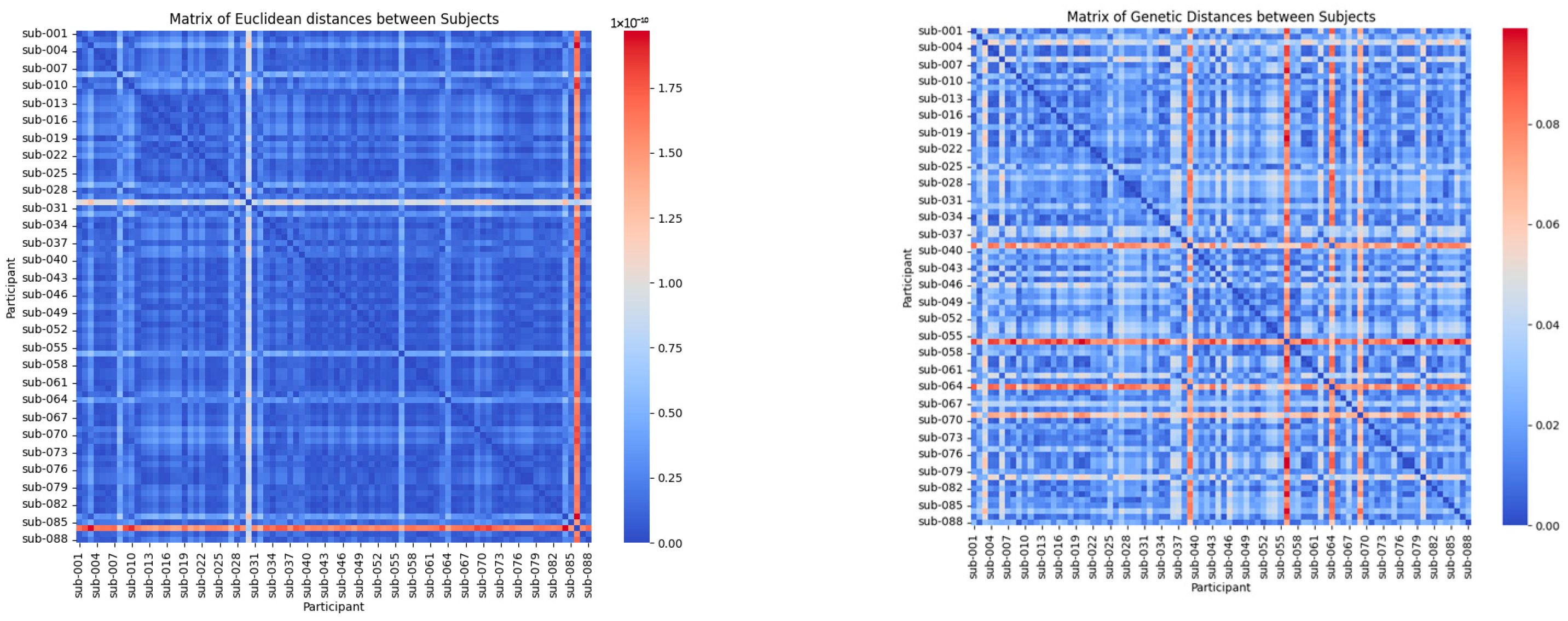
The heat maps in Figure 1 provide a visual representation of the relationships between the participants based on two distinct metrics: the Mahalanobis distance and the adapted genetic distance metric.
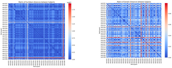
Figure 1.
Mahalanobis distance-based and metric distance-based.
The Mahalanobis distance-based heat map provides a global perspective of the multivariate variations between the participants by considering the correlations between the variables. In this visualization, lighter colours (closer to red) indicate significant differences in EEG signal patterns, while darker shades (closer to blue) represent higher similarity. This approach is particularly effective for identifying the broad patterns and trends across clinical groups, such as distinguishing participants with Alzheimer’s disease, frontotemporal dementia, and healthy controls. By offering a high-level overview, the Mahalanobis distance helps to cluster the participants based on shared characteristics, revealing the general relationships within the dataset.
The genetic distance-based heat map focuses on biologically relevant features, such as Delta, Theta, Alpha, and Beta band strengths, to capture the detailed differences and similarities between the participants. In this map, areas in shades of red highlight greater differences in EEG signals, while blue shades emphasize higher similarity. Unlike the Mahalanobis approach, this metric allows for the identification of finer intra-group variations, making it possible to detect specific subtypes within clinical groups. These subtypes may correlate with disease progression or individual variability, offering actionable insights for personalized medicine. This detailed perspective underscores the utility of the genetic distance metric in capturing clinically relevant patterns that might otherwise be overlooked.
The Mahalanobis distance provides a global perspective, clustering the participants into broader clinical groups, while the adapted genetic distance metric captures the fine-grained differences, enabling the identification of subtypes and detailed intra-group patterns. Together, these complementary metrics offer a comprehensive analysis, combining global variability insights with clinically relevant, detailed relationships.
This pattern allows for the identification of the similarities within the same clinical groups and the marked differences between the participants from different groups, providing an overview of how the data cluster according to the statistically relevant characteristics.
The heat map generated with the adapted genetic distance metric reflects the similarities and differences between the participants, prioritizing biological features such as Delta, Theta, Alpha, and Beta band strengths. The areas in shades of red highlight greater differences between EEG signals, while blue shades indicate greater similarity. This approach highlights the specific differences within the clinical groups, allowing the identification of the detailed patterns and potential subtypes that could be related to disease progression or individual variations.
The Mahalanobis distance provides a global view of the differences between the participants, which is useful for identifying the general patterns across the clinical groups. In contrast, the adapted genetic distance metric allows for capturing specific similarities and differences based on prioritized characteristics, making it a powerful tool for identifying the subtypes within the clinical groups. This is clearly reflected in the heat maps, where the genetic distance shows more detailed and potentially clinically relevant patterns.
At this stage, the classification of subtypes within each clinical group (Alzheimer’s, Dementia, and Control) was performed using clustering techniques, specifically the K-Means algorithm. The relevant features, including frequency band strengths (Delta, Theta, Alpha, and Beta) and basic statistical metrics (mean, standard deviation, and range), were selected. These features capture both brain electrical activity and signal variability, allowing for an accurate representation of the individual differences within each group. Each participant was assigned to one of the three subtypes identified in the analysis.
The clustering results highlight the symmetrical relationships identified within and across the groups, with the genetic distance metric effectively balancing the intra-group homogeneity and inter-group divergence. This balance allows for clearer distinctions between the subtypes, particularly in early-stage versus advanced neurological disorders.
The choice of three subtypes is guided by the hypothesis that EEG signals reflect distinct stages or levels of severity within each clinical condition. For Alzheimer’s disease, the subtypes correspond to progressive stages—early, intermediate, and advanced—enabling a detailed characterization of disease progression. In dementia, the subtypes may represent phenotypic variations or differential responses to treatment, reflecting the heterogeneity of the condition. For the control group, the subtypes likely capture individual differences, such as variability in age or cognitive status.
These findings provide valuable insights into the heterogeneity of the clinical groups. By identifying the subtypes within each group, this approach supports the development of personalized treatment strategies tailored to specific stages or phenotypes, offering a deeper understanding of the progression of and variability in neurological disorders.
Table 4 shows the distribution of subtypes within each clinical group (Alzheimer’s—A, Control—C, and Frontotemporal Dementia—F), reflecting how the participants were divided according to the characteristics of their EEG signals. The group column indicates the clinical group to which each participant belongs, while the subtype column corresponds to the subtype assigned to each individual based on the clustering analysis previously performed. The numbers column shows the number of participants within each subtype for each group.
Table 4.
Subtypes.
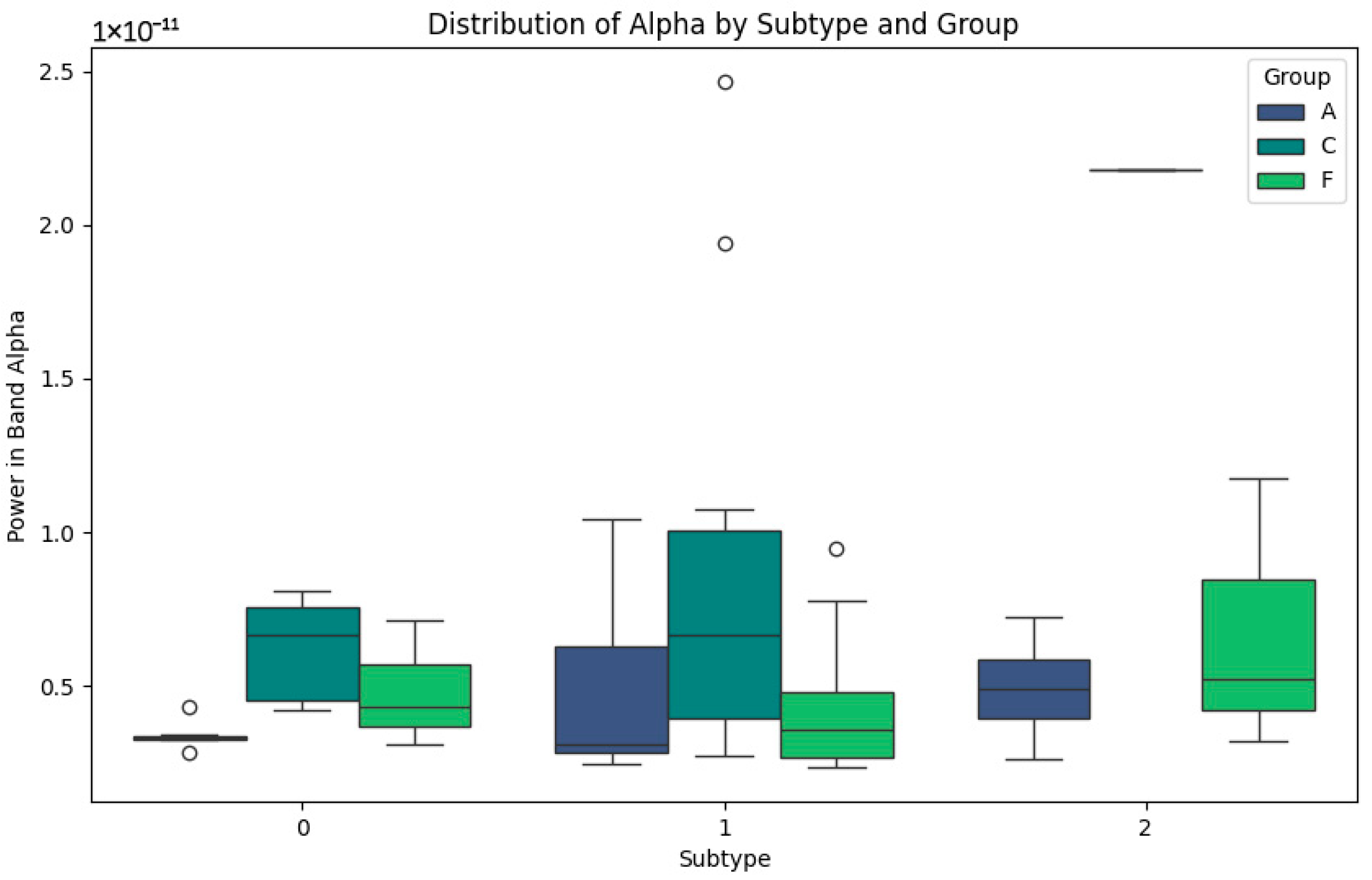
In Figure 2 representing the Alpha band, the differentiated patterns between the subtypes are highlighted. In subtype 0, power values are low for groups A (Alzheimer’s) and F (Frontotemporal Dementia), indicating the alterations in this band, possibly related to cognitive impairment. In contrast, the subjects in group C (Control) show slightly higher values, reflecting the stability in normal cortical activity. For subtype 1, group C shows a greater dispersion of Alpha powers, with higher maximum values, possibly reflecting a greater cognitive processing capacity. In subtype 2, group F values are more homogeneous, which may correlate with more consistent patterns of disease progression. This Alpha band analysis suggests that the differences in power are closely related to the levels of cognitive impairment and cortical activity, with the variability within the subtypes being indicative of the different clinical stages and subtypes defined in each group.

Figure 2.
Alpha-band subtypes.
Figure 3 shows faster and more specific cortical activity patterns. In subtype 0, the power values are low in all the groups, especially in group A, which could be indicative of advanced cognitive impairment. In group F, although the values are low, slight increases are observed which could be a sign of residual cortical activity. In subtype 1, group C maintains stable values and a lower dispersion, reflecting cortical processing typical of healthy subjects. On the other hand, in group F, high power peaks are identified, which could be related to compensatory cortical responses. In subtype 2, the Beta band shows higher values in group F, reflecting possible differences in neuronal activity that could be correlated with the specific features of frontotemporal dementia. In contrast, group A maintains consistently low levels, reaffirming its relationship with greater cortical involvement.
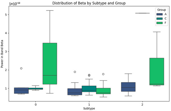
Figure 3.
Beta-band subtypes.
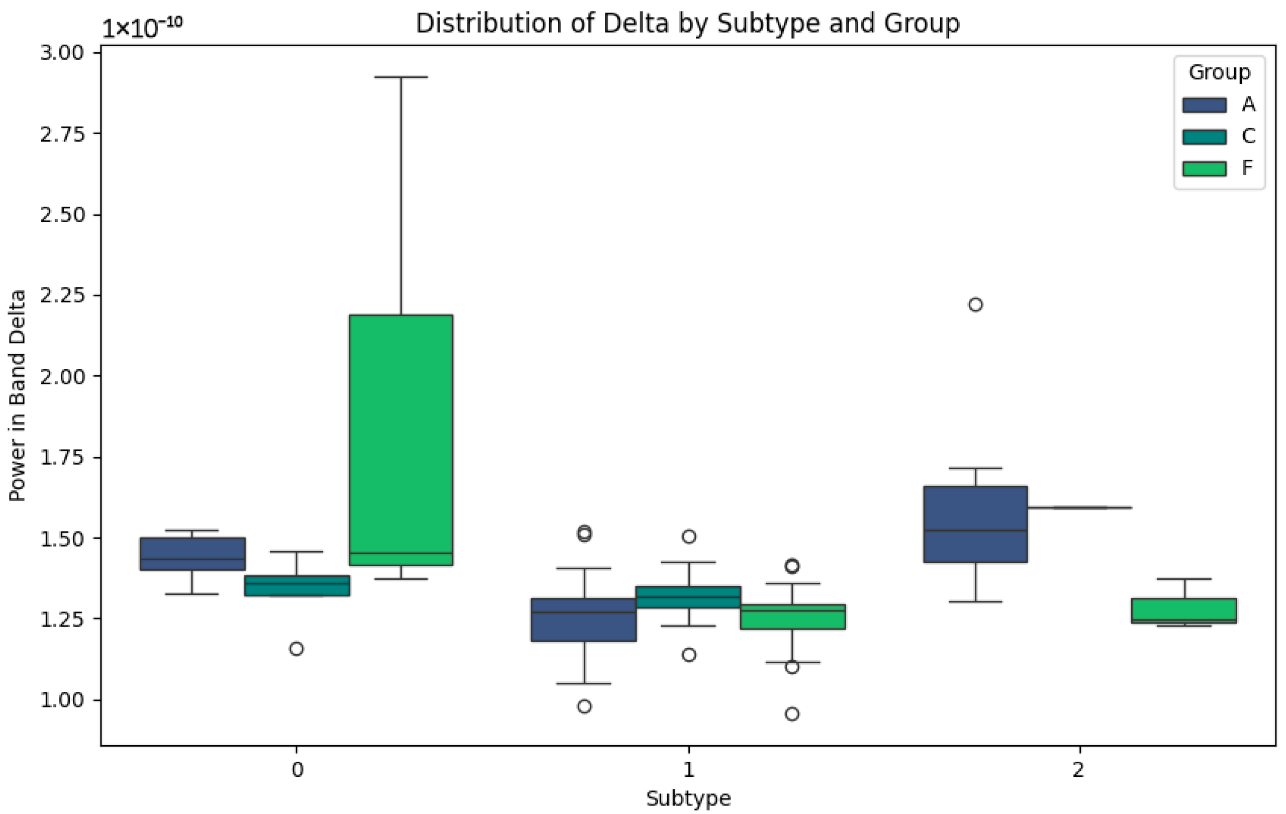
The Delta band, associated with slow waves and brain repair processes, presents interesting patterns in Figure 4. In subtype 0, group A shows higher values than C and F, possibly indicating an attempt at neuronal compensation in Alzheimer’s patients. In groups C and F, the lower values reflect more normal or less affected activity in this band. For subtype 1, elevated values are observed in group F, which could be representative of the particular features of frontotemporal dementia, such as distinct degenerative processes. In subtype 2, groups C and F show consistently low values, which could indicate stability or lesser involvement in this band. This behaviour contrasts with group A, where the values remain higher, possibly due to the compensatory responses in the advanced stages of the disease.

Figure 4.
Delta-band subtypes.
Figure 5 representing the Theta band, related to memory and attention, highlights the differences between the subtypes. In subtype 0, groups A and C show low power values, while group F shows slightly higher values, reflecting differential activity. In subtype 1, group F shows high variability, with high peaks of potency that could be associated with the compensatory responses or individual differences in disease progression. Finally, in subtype 2, the Theta power values are lower in group F, while group A maintains low but consistent values. This pattern could reflect the progressive impairment of the Theta band in neurodegenerative diseases and its relative stability in healthy subjects in group C.
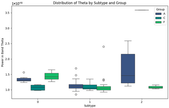
Figure 5.
Theta-band subtypes.
In the statistical analysis (Table 5), ANOVA tests were performed for each frequency band (Delta, Theta, Alpha, and Beta) within each clinical group (Alzheimer’s, Dementia, and Control). This approach allowed a comparison of the differences in the EEG signal characteristics between the subtypes previously identified via clustering. ANOVA tests assessed whether the observed differences in band strengths between the subtypes were statistically significant, providing a deeper understanding of the variability within each clinical group. The results are summarized in terms of the key statistical values, such as the F-statistic and p-values, which indicate the magnitude and significance of the differences between the subtypes. This statistical analysis not only supports the validity of the subtype classification, but also highlights the frequency bands most relevant for differentiation between the disease states and patterns in the control groups, helping to identify the potential markers of clinical progression or stability.
Table 5.
Statistical analysis.
By integrating the concept of symmetry into the genetic distance metric, this study not only advances the classification of the neurological subtypes but also underscores the importance of balanced variability representation in biomedical signal processing. Symmetry facilitates a holistic understanding of how brain signal patterns relate to disease progression, paving the way for personalized interventions.
5. Conclusions
The incorporation of symmetry into the genetic distance metric has proven instrumental in enhancing the subtype classification and understanding variability in neurological disorders. This study demonstrates how symmetry can be a powerful conceptual and analytical tool in biomedical signal analysis. The comparative analysis demonstrates that the genetic similarity metric not only captures the dynamic and non-linear properties of EEG signals but also enables the identification of the subtle signal variations linked to disease states. These findings underscore its potential for applications in neurological disorder monitoring and personalized treatment strategies.
Delta and Theta bands tend to increase as the disease progresses, while Alpha and Beta bands show a marked decrease, particularly in the Alzheimer’s and Dementia groups (Table 6). The analysis of subtypes through genetic distance and band-specific potencies allows the identification of the distinct patterns within each clinical group, providing a powerful tool for the classification and monitoring of disease progression.
Table 6.
Conclusions on bands.
This study establishes a promising basis for applying advanced tools in clinical practice and developing personalized treatments for neurological disorders such as Alzheimer’s disease and frontotemporal dementia. The integration of genetic distance with brain patterns and clinical subtypes allows us to better understand the progression of these diseases and to design therapeutic interventions tailored to the unique characteristics of each patient.
The identified subtypes offer valuable insights for designing personalized therapeutic strategies. By recognizing the distinct stages and phenotypes in Alzheimer’s disease and dementia, clinicians can tailor treatments to the specific needs of each subgroup, improving outcomes and resource allocation. This study provides a framework for translating the clustering results into targeted interventions, emphasizing the role of precision medicine in neurodegenerative disorders.
We recommend future research to assess the longitudinal evolution of subtypes and their response to specific treatments. It would also be useful to explore how environmental and lifestyle factors interact with genetic and brain patterns in the progression of neurological diseases. Correlating genetic distance with specific biomarkers represents an important step in broadening its clinical applicability. Among the biomarkers to prioritize in future studies are the following:
- Amyloid-beta levels, associated with the accumulation of amyloid plaques, which are a hallmark of Alzheimer’s disease.
- Tau protein levels, indicative of neurofibrillary tangles and neuronal degradation.
- Markers of neuroinflammation, such as cytokines, which are increasingly recognized as key players in neurological diseases.
Longitudinal analyses can enhance the model’s accuracy by capturing the dynamic changes in EEG signals and biomarkers over time. This approach provides a more comprehensive view of the disease progression, enabling the identification of early transition points in the disease state and improving predictive modelling. By focusing on intra-individual changes, longitudinal studies reduce the variability caused by inter-individual differences and improve the robustness of the findings.
Combining predictive models based on the genetic distance with specific brain patterns allows for the development of more precise and personalized treatments. This represents a step toward individualized medicine, maximizing the efficacy of interventions while minimizing the adverse effects. Future studies could leverage multi-modal data, including EEG, biomarkers, and environmental factors, to create integrated models capable of advancing the clinical applications and improving patient outcomes.
Author Contributions
Conceptualization, J.A.R.-V. and O.D.-P.; methodology, J.A.R.-V., R.A.B.-C., and M.A.M.-V.; software, E.S.-A. and J.C.R.-F.; validation, A.F.-P., M.A.R.-J. and J.M.X.-P.; formal analysis, O.D.-P.; investigation, J.A.R.-V. and M.A.M.-V.; resources, R.A.B.-C. and M.A.R.-J.; data curation, J.C.R.-F. and E.S.-A.; writing—original draft preparation, J.A.R.-V. and A.F.-P.; writing—review and editing, O.D.-P. and J.M.X.-P.; visualization, M.A.M.-V. and E.S.-A.; supervision, J.A.R.-V. and O.D.-P.; project administration, J.A.R.-V.; funding acquisition, R.A.B.-C. All authors have read and agreed to the published version of the manuscript.
Funding
This research received no external funding.
Data Availability Statement
The EEG dataset analyzed in this study is publicly available from the OpenNeuro repository at https://github.com/OpenNeuroDatasets/ds004504 (accessed on 19 January 2025). This dataset includes recordings from participants diagnosed with Alzheimer’s disease, frontotemporal dementia, and healthy controls. No new data were generated during this study.
Acknowledgments
The authors wish to express their gratitude to the Universidad Politécnica de Pachuca, LANAVEX, and CONAHCYT for their invaluable support in providing resources, facilities, and guidance throughout this research.
Conflicts of Interest
The authors declare no conflicts of interest.
References
- Ginsburg, G.S.; McCarthy, J.J. Personalized medicine: Revolutionizing drug discovery and patient care. Trends Biotechnol. 2001, 19, 491–496. [Google Scholar] [CrossRef] [PubMed]
- National Research Council. Toward Precision Medicine: Building a Knowledge Network for Biomedical Research and a New Taxonomy of Disease; The National Academies Press: Washington, DC, USA, 2011. [Google Scholar]
- Pérez-Ortega, J.; Pazos, R.A.; Ruiz-Vanoye, J.A.; Frausto-Solís, J.; González-Barbosa, J.; Fraire-Huacuja, H.; Díaz-Parra, O. A genetic distance metric to discriminate the selection of algorithms for the general ATSP problem. J. Intell. Fuzzy Syst. 2010, 21, 57–64. [Google Scholar] [CrossRef]
- Ginsburg, G.S.; Willard, H.F. Genomic and personalized medicine: Foundations and applications. Transl. Res. 2009, 154, 277–287. [Google Scholar] [CrossRef] [PubMed]
- Collins, F.S.; Varmus, H. A new initiative on precision medicine. N. Engl. J. Med. 2015, 372, 793–795. [Google Scholar] [CrossRef] [PubMed]
- Ashley, E.A. The precision medicine initiative: A new era of medicine. J. Am. Med. Assoc. 2016, 316, 1357–1358. [Google Scholar]
- Kahn, J.P.; Mastroianni, A.C. The ethics of precision medicine. Am. J. Bioeth. 2016, 16, 3–12. [Google Scholar]
- Zhang, Y.; Zhou, X. A modified Euclidean distance for feature weighting in pattern recognition. Pattern Recognit. Lett. 2015, 42, 80–86. [Google Scholar]
- Mahalanobis, P.C. On the generalized distance in statistics. Proc. Natl. Inst. Sci. India. 1936, 2, 49–55. [Google Scholar]
- Shannon, C.E. A mathematical theory of communication. Bell Syst. Tech. J. 1948, 27, 379–423. [Google Scholar] [CrossRef]
- Cavalli-Sforza, L.L.; Edwards, A.W.F. Phylogenetic analysis: Models and estimation procedures. Am. J. Hum. Genet. 1967, 19, 233–257. [Google Scholar]
- Rogers, J.S. Measures of genetic similarity and genetic distances. Stud. Genet. VII 1972, 7213, 145–153. [Google Scholar]
- Relethford, J.H. Genetic drift can obscure population history: Problem and solution. Hum. Biol. 1996, 68, 29–44. [Google Scholar] [PubMed]
- Harpending, H.C.; Jenkins, T. Genetic distance among southern African populations. In Methods and Theories of Anthropological Genetics; Crawford, M.H., Workman, P.L., Eds.; University of New Mexico Press: Albuquerque, NC, USA, 1973; pp. 177–199. [Google Scholar]
- Takezaki, N.; Nei, M. Empirical tests of the reliability of phylogenetic trees constructed with microsatellite DNA. Genetics 1996, 178, 385–392. [Google Scholar] [CrossRef]
- Belle, E.M.; Barbujani, G. Worldwide analysis of multiple microsatellites: Language diversity has a detectable influence on DNA diversity. Am. J. Phys. Anthropol. 2007, 133, 1137–1146. [Google Scholar] [CrossRef]
- Paixão, T.; Phadke, S.; Azevedo, R.; Zufall, R. Sex ratio evolution under probabilistic sex determination. Evolution 2011, 65, 2050–2060. [Google Scholar] [CrossRef]
- Engelsma, K.A.; Calus, M.P.; Bijma, P.; Windig, J.J. Estimating genetic diversity across the neutral genome with the use of dense marker maps. Genet. Sel. Evol. 2010, 42, 12. [Google Scholar] [CrossRef]
- Liu, C.; Yu, D.; Ma, X.; Xie, S.; Zhang, H. Neural evidence for image quality perception based on algebraic topology. PLoS ONE 2021, 16, e0261223. [Google Scholar] [CrossRef]
- Simons, S.; Espino, P.; Abásolo, D. Fuzzy entropy analysis of the electroencephalogram in patients with Alzheimer’s disease: Is the method superior to sample entropy? Entropy 2018, 20, 21. [Google Scholar] [CrossRef]
- Groppe, D.M.; Bickel, S.; Keller, C.J.; Jain, S.K.; Hwang, S.T.; Harden, C.; Mehta, A.D. Dominant frequencies of resting human brain activity as measured by the electrocorticogram. NeuroImage 2013, 79, 223–233. [Google Scholar] [CrossRef]
- Zhao, L.; Wei, S.; Tang, H.; Liu, C. Multivariable fuzzy measure entropy analysis for heart rate variability and heart sound amplitude variability. Entropy 2016, 18, 430. [Google Scholar] [CrossRef]
- Nieto-del-Amor, F.; Beskhani, R.; Ye-Lin, Y.; Garcia-Casado, J.; Diaz-Martinez, A.; Monfort-Ortiz, R.; Diago-Almela, V.J.; Hao, D.; Prats-Boluda, G. Assessment of dispersion and bubble entropy measures for enhancing preterm birth prediction based on electrohysterographic signals. Sensors 2021, 21, 6071. [Google Scholar] [CrossRef] [PubMed]
- Walker, M.P.; Ayre, G.; Perry, E.; Wesnes, K.; McKeith, I.; Tovee, M.; Edwardson, J.; Ballard, C. Quantification and characterisation of fluctuating cognition in dementia with Lewy bodies and Alzheimer’s disease. Dement. Geriatr. Cogn. Disord. 2000, 11, 327–335. [Google Scholar] [CrossRef] [PubMed]
- Zieselman, A.L.; Fisher, J.; Hu, T.; Andrews, P.C.; Greene, C.S.; Shen, L.; Saykin, A.J.; Moore, J.H.; for the Alzheimer’s Disease Neuroimaging Initiative. Computational genetics analysis of grey matter density in Alzheimer’s disease. BioData Min. 2014, 7, 17. [Google Scholar] [CrossRef]
- Qiang, Z.; Duan, K.; Miao, Y.; Tan, J. Identification of genetic markers and immune infiltration characteristics of Alzheimer’s disease through weighted gene co-expression network analysis. Front. Neurol. 2022, 13, 947781. [Google Scholar] [CrossRef]
- Zhou, K.; Wang, L.; Wu, L.; Wu, Q.; Zhu, L.; Yang, X.; Li, D. Key genes associated with Alzheimer’s disease and periodontitis. Preprint 2022. [Google Scholar] [CrossRef]
- Pluta, R.; Ułamek-Kozioł, M.; Januszewski, S.; Czuczwar, S.J. From brain ischemia to Alzheimer-like neurodegeneration. Neuropsychiatry 2018, 8, 1000510. [Google Scholar] [CrossRef]
- Weiner, M.W.; Veitch, D.P.; Aisen, P.S.; Beckett, L.A.; Cairns, N.J.; Green, R.C.; Harvey, D.; Jack, C.R.; Jagust, W.; Liu, E.; et al. The Alzheimer’s Disease Neuroimaging Initiative: A review of papers published since its inception. Alzheimer’s Dement. 2022, 18, e63–e73. [Google Scholar]
- Kim, H.; Jung, S.; Kim, J.; Jang, H.; Kang, S.H.; Hwangbo, S.; Kim, J.P.; Kim, S.Y.; Kim, B.; Kim, S.; et al. Identifying novel genetic variants for brain amyloid deposition: A genome-wide association study in the Korean population. Alzheimer’s Res. Ther. 2021, 13, e854. [Google Scholar] [CrossRef]
- Johansen, M.; Joensen, S.; Restorff, M.; Stórá, T.; Christy, D.; Gustavsson, E.K.; Bian, J.; Guo, Y.; Farrer, M.J.; Petersen, M.S. Polygenic risk of Alzheimer’s disease in the Faroe Islands. Eur. J. Neurol. 2022, 29, 2192–2200. [Google Scholar] [CrossRef]
- Lumsden, A.; Mulugeta, A.; Zhou, A.; Hyppönen, E. Apolipoprotein E (APOE) genotype-associated disease risks: A phenome-wide, registry-based, case-control study utilising the UK Biobank. EBioMedicine 2020, 59, e102954. [Google Scholar] [CrossRef]
- Law, Z.K.; Todd, C.; Mehraram, R.; Schumacher, J.; Baker, M.R.; LeBeau, F.E.N.; Yarnall, A.; Onofrj, M.; Bonanni, L.; Thomas, A.; et al. The role of EEG in the diagnosis, prognosis and clinical correlations of dementia with Lewy bodies: A systematic review. Diagnostics 2020, 10, 616. [Google Scholar] [CrossRef] [PubMed]
- Ahmed, A.H.M.; Ahmed, K.A.H.M.; Omer, M.E.A.; Siddig, A.A. Incidence of epilepsy among elderly Sudanese patients with Alzheimer’s disease: A prospective cohort study on 480 patients, Khartoum, Sudan. Preprint 2021. [Google Scholar] [CrossRef]
- Miltiadous, A.; Tzimourta, K.D.; Afrantou, T.; Ioannidis, P.; Grigoriadis, N.; Tsalikakis, D.G.; Angelidis, P.; Tsipouras, M.G.; Glavas, E.; Giannakeas, N.; et al. A dataset of scalp EEG recordings of Alzheimer’s disease, frontotemporal dementia and healthy subjects from routine EEG. Data 2023, 8, 95. [Google Scholar] [CrossRef]
- Wan, K.; Ma, Z.; Zhou, X.; Zhang, Y.-M.; Yu, X.-F.; You, M.-Z.; Huang, C.-J.; Zhang, W.; Sun, Z.-W. A novel probable pathogenic PSEN2 mutation p.Phe369Ser associated with early-onset Alzheimer’s disease in a Chinese Han family: A case report. Front. Aging Neurosci. 2021, 13, e710075. [Google Scholar] [CrossRef]
- Mendez, M.F. Early-onset Alzheimer’s disease. Neurol. Clin. 2017, 35, 263–281. [Google Scholar] [CrossRef]
- Tort-Merino, A.; Falgàs, N.; Allen, I.E.; Balasa, M.; Olives, J.; Contador, J.; Castellví, M.; Juncà-Parella, J.; Guillén, N.; Borrego-Écija, S.; et al. Early-onset Alzheimer’s disease shows a distinct neuropsychological profile and more aggressive trajectories of cognitive decline than late-onset. Ann. Clin. Transl. Neurol. 2022, 9, 1962–1973. [Google Scholar] [CrossRef]
- Falgàs, N.; Allen, I.E.; Spina, S.; Grant, H.; Escudero, S.D.P.; Merrilees, J.; Gearhart, R.; Rosen, H.J.; Kramer, J.H.; Seeley, W.W.; et al. The severity of neuropsychiatric symptoms is higher in early-onset than late-onset Alzheimer’s disease. Eur. J. Neurol. 2021, 29, 957–967. [Google Scholar] [CrossRef]
- Wolk, D.A. Amyloid imaging in atypical presentations of Alzheimer’s disease. Curr. Neurol. Neurosci. Rep. 2013, 13, e412. [Google Scholar] [CrossRef]
- Tsantzali, I.; Paraskevas, P.; Paraskevas, S.; Paraskevas, S.G.; Efthimiopoulos, S.; Tsivgoulis, G. Atypical presentations of Alzheimer’s disease: Beyond amnestic dementia. Clin. Exp. Investig. 2020, 1–4. [Google Scholar]
- Sakae, N.; Josephs, K.; Litvan, I.; Murray, M.E.; Duara, R.; Uitti, R.J.; Wszolek, Z.K.; van Gerpen, J.; Graff-Radford, N.R.; Dickson, D.W. Clinicopathologic subtype of Alzheimer’s disease presenting as corticobasal syndrome. Alzheimer’s Dement. 2019, 15, 1218–1228. [Google Scholar] [CrossRef]
- Ferrari-Souza, J.; Brum, W.; Hauschild, L.; Da Ros, L.U.; Ferreira, P.C.L.; Bellaver, B.; Leffa, D.T.; Bieger, A.; Tissot, C.; Lussier, F.Z.; et al. Vascular risk burden is a key player in the early progression of Alzheimer’s disease. Neurobiol. Aging 2024, 136, 88–98. [Google Scholar] [CrossRef] [PubMed]
- Bangen, K.J.; Nation, D.A.; Delano-Wood, L.; Da Ros, L.U.; Ferreira, P.C.L.; Bellaver, B.; Leffa, D.T.; Bieger, A.; Tissot, C.; Lussier, F.Z.; et al. Aggregate effects of vascular risk factors on cerebrovascular changes in autopsy-confirmed Alzheimer’s disease. Alzheimer’s Dement. 2014, 11, 394. [Google Scholar] [CrossRef] [PubMed]
- Ewers, M.; Mielke, M.M.; Hampel, H. Blood-based biomarkers of microvascular pathology in Alzheimer’s disease. Exp. Gerontol. 2010, 45, 75–79. [Google Scholar] [CrossRef] [PubMed]
- Kowalska, A.; Pruchnik-Wolińska, D.; Florczak, J.; Modestowicz, R.; Szczech, J.; Kozubski, W.; Rossa, G.; Wender, M. Genetic study of familial cases of Alzheimer’s disease. Acta Biochim. Pol. 2004, 51, 245–252. [Google Scholar] [CrossRef]
- Finckh, U.; Kuschel, C.; Anagnostouli, M.; Patsouris, E.; Pantes, G.V.; Gatzonis, S.; Kapaki, E.; Davaki, P.; Lamszus, K.; Stavrou, D.; et al. Novel mutations and repeated findings of mutations in familial Alzheimer disease. Neurogenetics 2005, 6, 85–89. [Google Scholar] [CrossRef]
- Rosenthal, S.L.; Kamboh, M.I. Late-onset Alzheimer’s disease genes and the potentially implicated pathways. Curr. Genet. Med. Rep. 2014, 2, 85–101. [Google Scholar] [CrossRef]
- Sherrington, R.; Rogaev, E.I.; Liang, Y.; Rogaeva, E.A.; Levesque, G.; Ikeda, M.; Chi, H.; Lin, C.; Li, G.; Holman, K.; et al. Cloning of a gene bearing missense mutations in early-onset familial Alzheimer’s disease. Nature 1995, 375, 754–760. [Google Scholar] [CrossRef]
- Goate, A.; Chartier-Harlin, M.C.; Mullan, M.; Brown, J.; Crawford, F.; Fidani, L.; Giuffra, L.; Haynes, A.; Irving, N.; James, L.; et al. Segregation of a missense mutation in the amyloid precursor protein gene with familial Alzheimer’s disease. Nature 1991, 349, 704–706. [Google Scholar] [CrossRef]
- Selkoe, D.J. The genetics and molecular pathology of Alzheimer’s disease: Roles of amyloid and the presenilins. Neuron 1997, 19, 1151–1154. [Google Scholar]
- Murray, M.E.; Graff-Radford, N.R.; Ross, O.A.; Petersen, R.C.; Duara, R.; Dickson, D.W. Neuropathologically defined subtypes of Alzheimer’s disease with distinct clinical characteristics: A retrospective study. Lancet Neurol. 2011, 10, 785–796. [Google Scholar] [CrossRef]
- Arriagada, J.; Villalobos, R. Proteína tau como biomarcador en Alzheimer preclínico. ARS Medica Rev. Cienc. Médicas 2022, 47, 56–67. [Google Scholar] [CrossRef]
- Reiman, E.M.; Quiroz, Y.T.; Fleisher, A.S.; Chen, K.; Velez-Pardo, C.; Jimenez-Del-Rio, M.; Fagan, A.M.; Shah, A.R.; Alvarez, S.; Arbelaez, A.; et al. Brain imaging and fluid biomarker analysis in young adults at genetic risk for autosomal dominant Alzheimer’s disease in the Presenilin 1 E280A kindred: A case-control study. Lancet Neurol. 2012, 11, 1048–1056. [Google Scholar] [CrossRef]
- OpenNeuro. A Dataset of EEG Recordings from: Alzheimer’s Disease, Frontotemporal Dementia and Healthy Subjects. Available online: https://github.com/OpenNeuroDatasets/ds004504. (accessed on 26 November 2024).


Disclaimer/Publisher’s Note: The statements, opinions and data contained in all publications are solely those of the individual author(s) and contributor(s) and not of MDPI and/or the editor(s). MDPI and/or the editor(s) disclaim responsibility for any injury to people or property resulting from any ideas, methods, instructions or products referred to in the content. |
© 2025 by the authors. Licensee MDPI, Basel, Switzerland. This article is an open access article distributed under the terms and conditions of the Creative Commons Attribution (CC BY) license (https://creativecommons.org/licenses/by/4.0/).