Abstract
Using a Dyson–Schwinger approach, we perform an analysis of the non-trivial ground state of thermal Yang–Mills theory in the non-perturbative regime where chiral symmetry is dynamically broken by a mass gap. Basic thermodynamic observables such as energy density and pressure are derived analytically, using Jacobi elliptic functions. The results are compared with the lattice results. Good agreement is found at low temperatures, providing a viable scenario for a gas of massive glue states populating higher levels of the spectrum of the theory. At high temperatures, a scenario without glue states consistent with a massive scalar field is observed, showing an interesting agreement with lattice data. The possibility is discussed that the results derived in this analysis open up a novel pathway beyond lattice to precision studies of phase transitions with false vacuum and cosmological relics that depend on the equations of state in strong coupled gauge theories of the type of Quantum Chromodynamics (QCD).
1. Introduction
Nowadays, only lattice simulations and other very limited theoretical approaches can reliably analyze the key observables in quantum Yang–Mills theories at finite temperatures in the strong coupling regime. Existing analytic methods such as the Polyakov loop model [1,2] still rely on sets of unknown non-perturbative parameters in the effective potential obtained by properly fitting lattice data. The exact form of the coefficients of a thermodynamic potential is found by an appropriate fit to the corresponding lattice data [3], which fully determines this potential for a given theory. Such a lattice-inspired effective model has been extensively employed in view of cosmological studies involving dark sectors (see, e.g., Ref. [4]).
In this work, we develop an approach enabling a fully analytical treatment of non-perturbative quantum field thermodynamics in terms of physical parameters alone. Our technique provides, in principle, a systematic way of incorporating finite temperature corrections to the exact Green function in the framework of a Dyson–Schwinger approach with a non-trivial ground state [5,6,7,8]. We consider a pure Yang–Mills theory, i.e., a gauge theory that has no other degrees of freedom than its potentials. It should be noted that Yang–Mills theories appear in nature only in interaction with other fields like fermions and scalars, such as in the Standard Model or QCD. Therefore, the idealized situation without other fields we consider here can only be compared to lattice calculations [9,10]. We demonstrate the robustness of our method by computing the effective action of a pure Yang–Mills quantum thermal theory under the symmetry group in the non-perturbative regime. The latter is then used to estimate some of the basic thermodynamic observables such as energy density and pressure. This is achieved by computing the effective energy–momentum tensor of the Yang–Mills theory and evaluating the thermal averages of its components in terms of the correlation functions [11,12]. Comparing the thermodynamic observables with the lattice data available for or colors [3] reveals an overall consistency in our results, suggesting that our method captures the most essential features of non-perturbative Yang–Mills dynamics at low temperatures. A recent approach with a free gas of glueballs shows a similar consistency [13]. As pure Yang–Mills theory is not seen in experiments, we emphasize that a proof of principle of the symmetry breaking in Yang–Mills theory can only be obtained by comparison with lattice calculations [3]. Our aim is to show how, from calculations based on the full theory, very good fits can be obtained at low and high temperatures, providing a sound physical interpretation for the lattice results.
To properly frame this work, we study a Yang–Mills theory without interactions with other fields like quarks or scalars. This is done by starting with the full theory and developing an exact solution that is afterwards fitted to the lattice results presented in Ref. [3]. This procedure should prove the soundness of our technique for thermal field theory too. It should be emphasized that, at low temperatures, the results presented in Ref. [3] are too few to obtain a significant result beyond and Yang–Mills theories. Therefore, we limit our analysis to these cases.
The paper is structured as follows. In Section 2, we present our technique to obtain an exact solution of the quantum Yang–Mills theory. In Section 3, we show how the partition function is obtained in our case. In Section 4, we derive all the thermodynamic variables for the Yang–Mills theory. In Section 5, we evaluate the partition function and present our results in comparison with lattice data. Finally, in Section 6, we give our conclusions.
2. Gaussian Solution of Quantum Yang–Mills Theory
We study an exact solution of the quantum Yang–Mills field theory that provides a Gaussian partition function [5,6,7,8,14]. It is worthwhile to study such a solution because exact solutions in quantum field theory are quite rare and are mostly given for non-physical models alone. We expect that the solution found here represents the behavior of the Yang–Mills theory. In order to simplify the presentation, we consider a Yang–Mills theory with a gauge group. The action at the classical level is given by
(latin letters represent group indices taking the values ), where is a generic source and an element of the algebra. The field strength tensor is given by
where g is the coupling constant and are the structure constants of the gauge group, leading to the classical equations of motion given by
In the following, we will provide a solution to Equation (3). The classical equation of motion generalizes to the quantum case by introducing a gauge fixing term and ghost fields and by considering the partition function (also known as the generating functional, cf., e.g., Ref. [15])
From the partition function, we can derive the pure correlation functions
and mixed correlation functions, for instance,
Our aim is to find a Gaussian solution where all the correlation functions can be expressed by and , given the expectation values of the gauge field, that is, the cumulant expansion of the partition function. It should be emphasized that the first two Dyson–Schwinger equations give the analogues of the classical equations of motion and the propagator of the theory, respectively, if the quantum corrections are properly accounted for.
This aim can be achieved by solving the Dyson–Schwinger Equations [5,6,7,8]
and
To solve these equations, we use a mapping theorem on the solutions of the classical Yang–Mills equations of motion [16,17] in order to take all components for the 1P-correlation function as equal,
where are sets of constants (e.g., for ), and is a scalar field to be determined. We also take
where we have made explicit the projector, and is a scalar propagator to be determined. Anticipating this ansatz, the anti-symmetry of was already used in Equations (7) and (8). In doing so, we are able to obtain both and in closed form and, in principle, compute the partition function at any desired order for this Gaussian solution. By direct substitution, we see immediately that
with . As is a constant, we can identify this as a mass correction that arises from quantum effects,
In the following, we will neglect this correction that, after renormalization, is assumed to have a small effect on the spectrum of the theory [7]. The two-point correlation function we obtain is translation invariant. We show this in Appendix A. Though the description of the Yang–Mills theory by a Lagrange density invariant unveils a symmetry under the gauge group that is broken by the introduction of the gauge fixing parameter, this is not the symmetry we concentrate on in this paper. Instead, we investigate the breaking of the chiral symmetry of this theory by a mass gap generated dynamically.
3. Partition Function in the IR Regime
Neglecting the mass correction, the solution for and can be obtained by taking
in terms of integration constants and , where the gluon momentum p satisfies the dispersion relation , and is the Jacobi elliptic function of the first kind with parameter . In our approach, is treated as a background field or as a specific non-trivial vacuum. For more details on the solution, cf. Appendix B.
In a first approximation that holds in the infrared (IR) limit of the Yang–Mills theory (confined phase), our approach allows us to truncate the functional series derived from Equation (4) at the quadratic term with the exact translationally invariant two-point function , while the three- and four-point functions are represented as products of one- and two-point functions evaluated at different points. Because of this, the theory is manifestly translation invariant at the level of observables where the Lehmann–Symanzik–Zimmermann reduction formula is assumed to hold.
In the considered approximation with the partition function truncated at the quadratic order, the IR truncated partition function reads [18]
The momentum space propagator in the Feynman gauge takes the shape
(see Appendix A for a derivation), where
and the mass spectrum reads
in terms of the mass of the lowest excitation, . Note that is a physical parameter in the same way as the scale of asymptotic freedom is generated dynamically in QCD by perturbation theory. We can identify this parameter with the string tension normally evaluated at . Stopping to the two-point correlation function, one obtains
Due to the sum, this is equivalent to a product of partition functions of an infinite set of scalar fields (i.e., glue states of mass ), each with weight (the factor 2 arises from the Minkowski metric, assuming all the currents are equal). Such a truncation represents a gas of free massive glue states. For such a gas, we expect a very good agreement at low temperatures, as we will see below. Finally, one can use the functional identity
Turning back to the partition function of each of the scalar field separately, one can write the Yang–Mills partition function in Equation (14) as
up to an overall multiplicative constant that is irrelevant for further considerations. Indeed, the source-free Yang–Mills partition function in the non-perturbative regime can be seen as a partition function of a system of infinitely many free scalar fields, where each field contributes with different weights, depending on its mass determined by Equation (20).
We see that, in the IR limit, the spectrum of the theory is quite different from that of the UV limit, where the true states of the theory are massless gluons and we have asymptotic freedom. In the IR limit, we have an infinite spectrum of massive particles that, in our approximation, are not interacting with each other. If we also use this spectrum for the regime of asymptotic freedom as well, i.e., for high temperatures, this will yield an infinite free energy for the model. We will see that for the high-temperature limit, the omission of the gluon states beyond the lowest one is a fairly good approximation.
4. Thermal Yang–Mills Theory
In what follows, we aim to derive the basic thermodynamic properties of the thermal Yang–Mills theory. Note that Equation (20) is the partition function of an infinite number of free scalar fields. Raised to the exponent, the product over the scalar fields adds a further sum over the scalar field modes. In the imaginary-time formulation, Equation (20) can be rewritten as [19]
where (with ) are the Matsubara frequencies. Furthermore, making use of the representation
with , performing the summation
and turning to the continuum limit for momentum in the system of volume V, we arrive at the final form for the partition function of the thermal Yang–Mills theory, given by
Here, the first expression in square brackets represents the contribution of the zero-point fluctuations of fields with mass in the ground state. In general, the vacuum term does not affect the thermodynamic observables in the thermal equilibrium but effectively renormalizes the physical observables by absorbing divergences emerging in the summation over k as , such that the physics is recovered through a finite, properly regulated, partition function, .
For further considerations, it is instructive to turn to a more compact representation in terms of a dimensionless variable (with ), such that
where a proper regularization of the summation is implied, is the standard thermal integral for a given state with mass defined in Equation (17), is the inverse of the temperature measured in units of the mass gap , and is the pressure of the free gluon gas. In what follows, we are interested in analyzing such thermodynamic observables of the quantum Yang–Mills fields like pressure
which is essentially the (normalized) partition function (cf. Equation (23)), and energy density
as well as the trace of the energy-momentum tensor (trace anomaly), .
The characteristic energy scale for the Yang–Mills theory will enter our analysis through the ratio , where is the mass gap of the theory and the critical temperature of the phase transition, which will be the only parameter to be fitted against the lattice data. The critical temperature is known from lattice data being around for and around for , according to Ref. [20].
5. Evaluation of the Partition Function
In order to determine the pressure and energy density, we have to evaluate . This is known in series form as
(see Appendix C for a derivation), where is a modified Bessel function. In the low-temperature limit, no convergence problems arise, and the series can be trusted enough for a comparison with lattice data. On the other hand, for , i.e., the high-temperature limit, this is no longer true for the series (29), as it should be expected by the infinite spectrum of free particles we are considering. The reason is that we are using an IR approximate solution to evaluate the UV limit of the Yang–Mills theory. This would be possible only by setting the mass gap of the theory to zero.
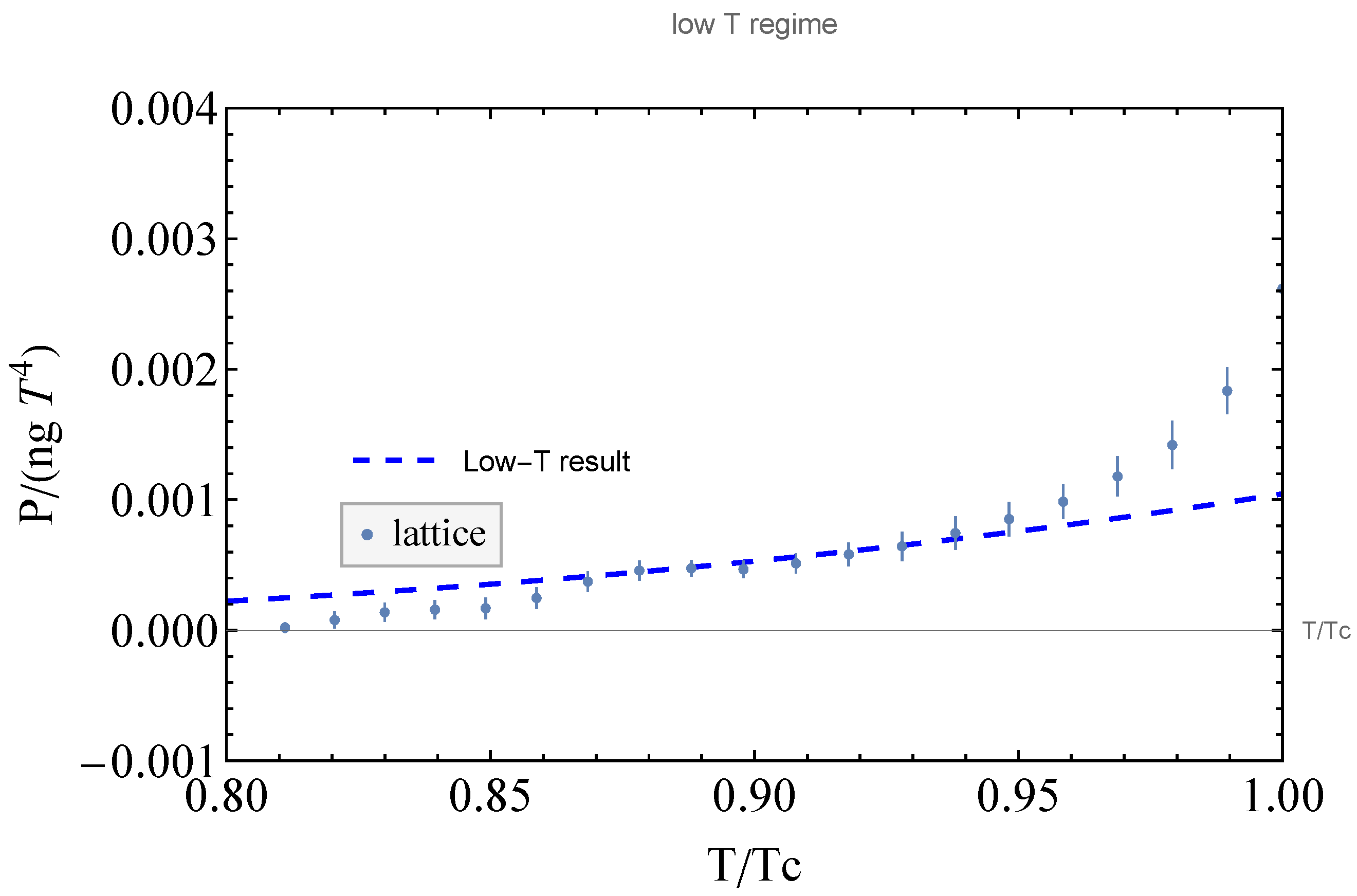
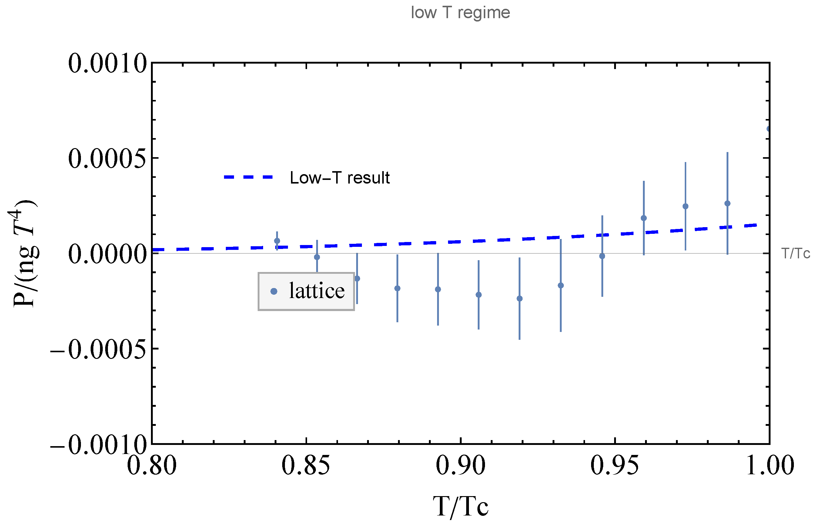
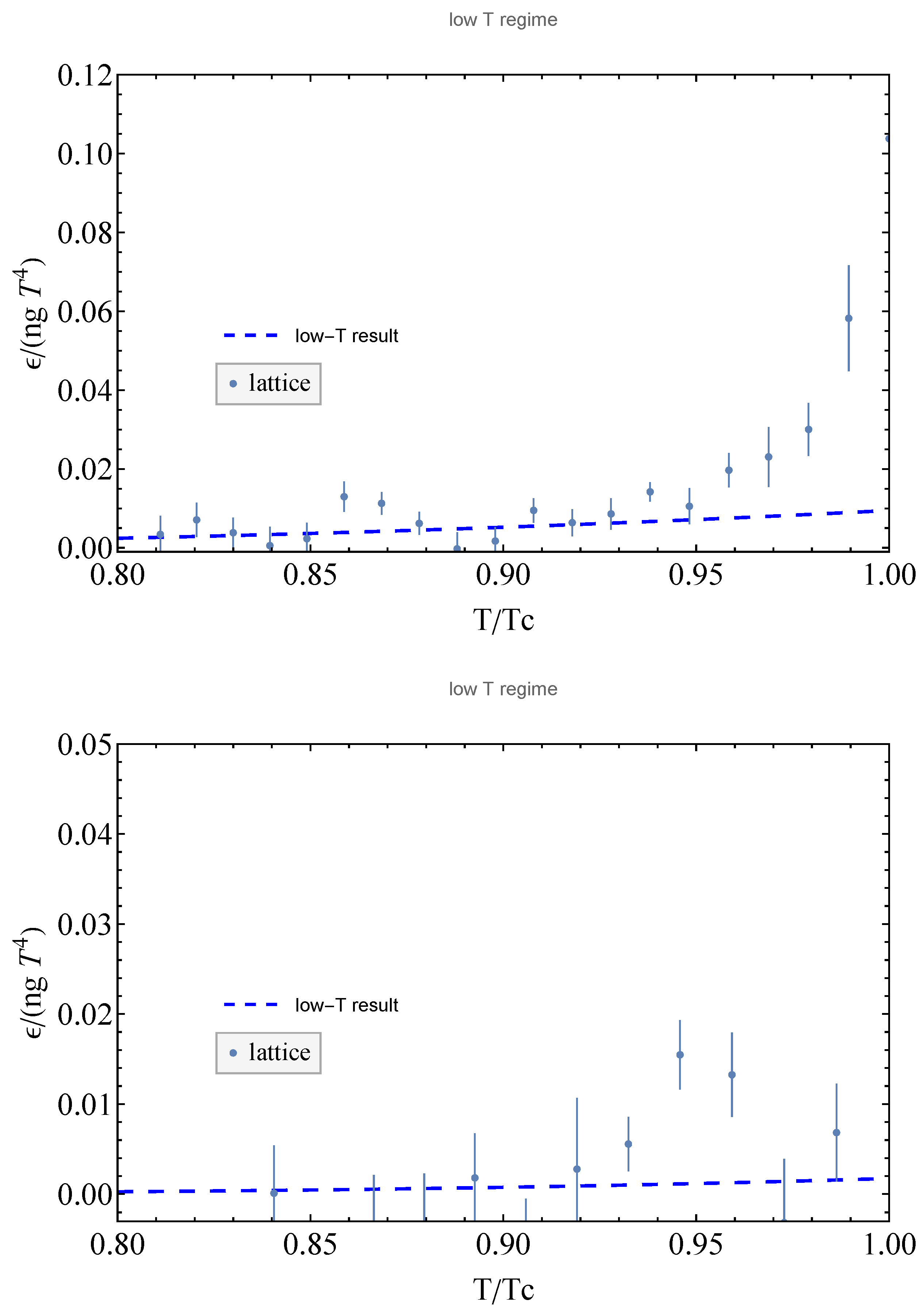
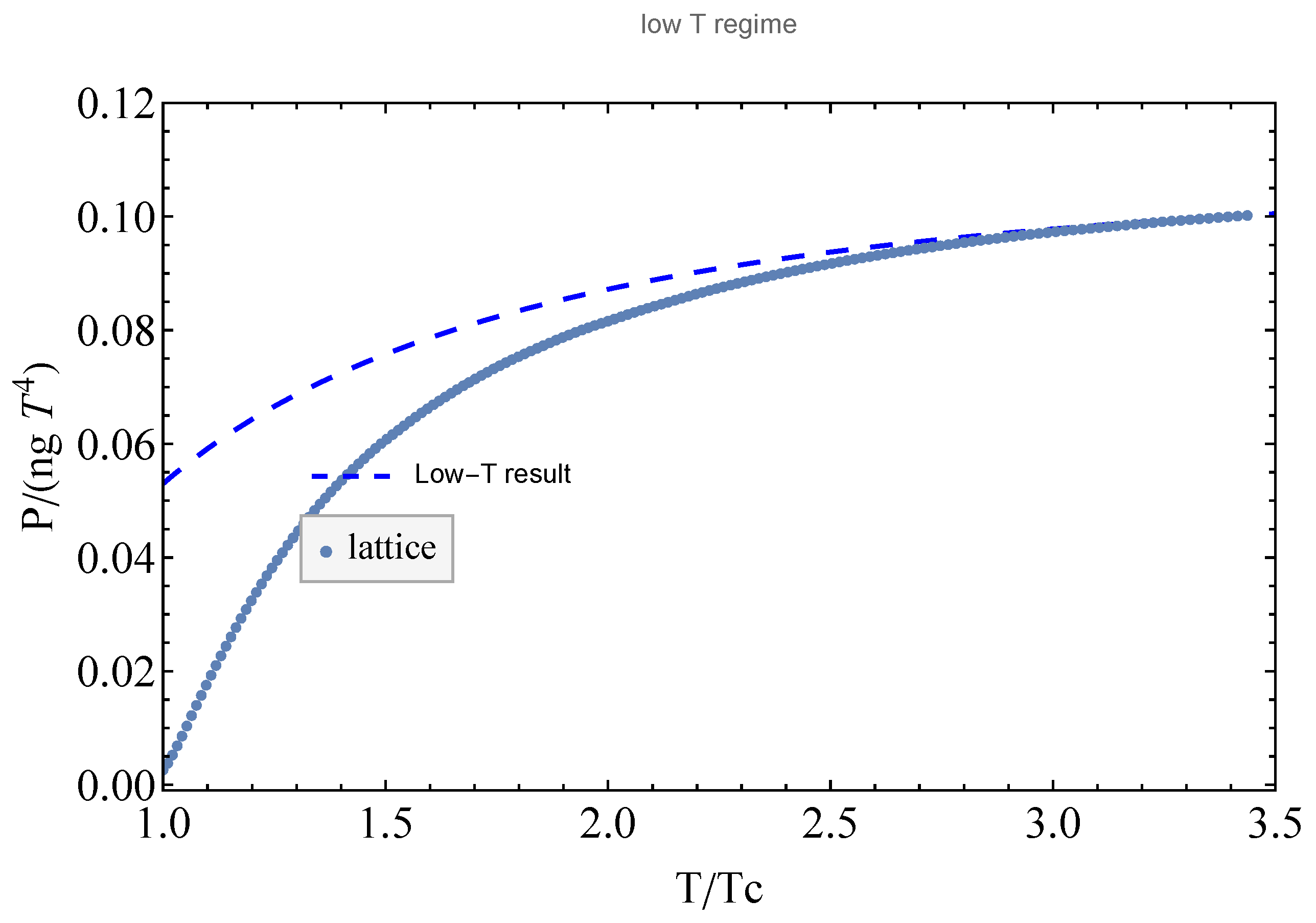
In the following plots, we compare our results for the pressure and the energy density for and with those from the lattice. As a single fitting parameter for both plots, we use the ratio . For the pressure displayed in Figure 1, we see a fairly good approximation , where is the mass gap for . Both masses are obtained independently by a fit. Because of this, they already take into account the number of colors. For the energy density, we obtain the result shown in Figure 2. Again, we have good agreement, with the dependency on the number of colors being the same as that for the pressure. We see that the ratio , both for the pressure and energy density, is very similar within the errors of the corresponding fits.
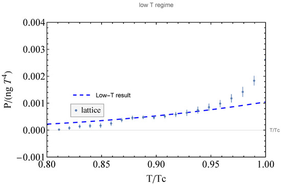
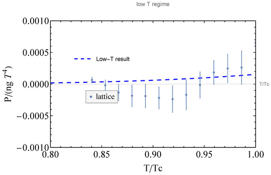
Figure 1.
Upper: Plot of the pressure p for with the fitted ratio compared to the lattice data. Lower: The same for with the fitted ratio .
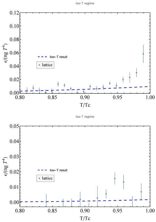
Figure 2.
Upper: Plot of the energy density for with the fitted ratio compared to the lattice data. Lower: The same for with the fitted ratio .
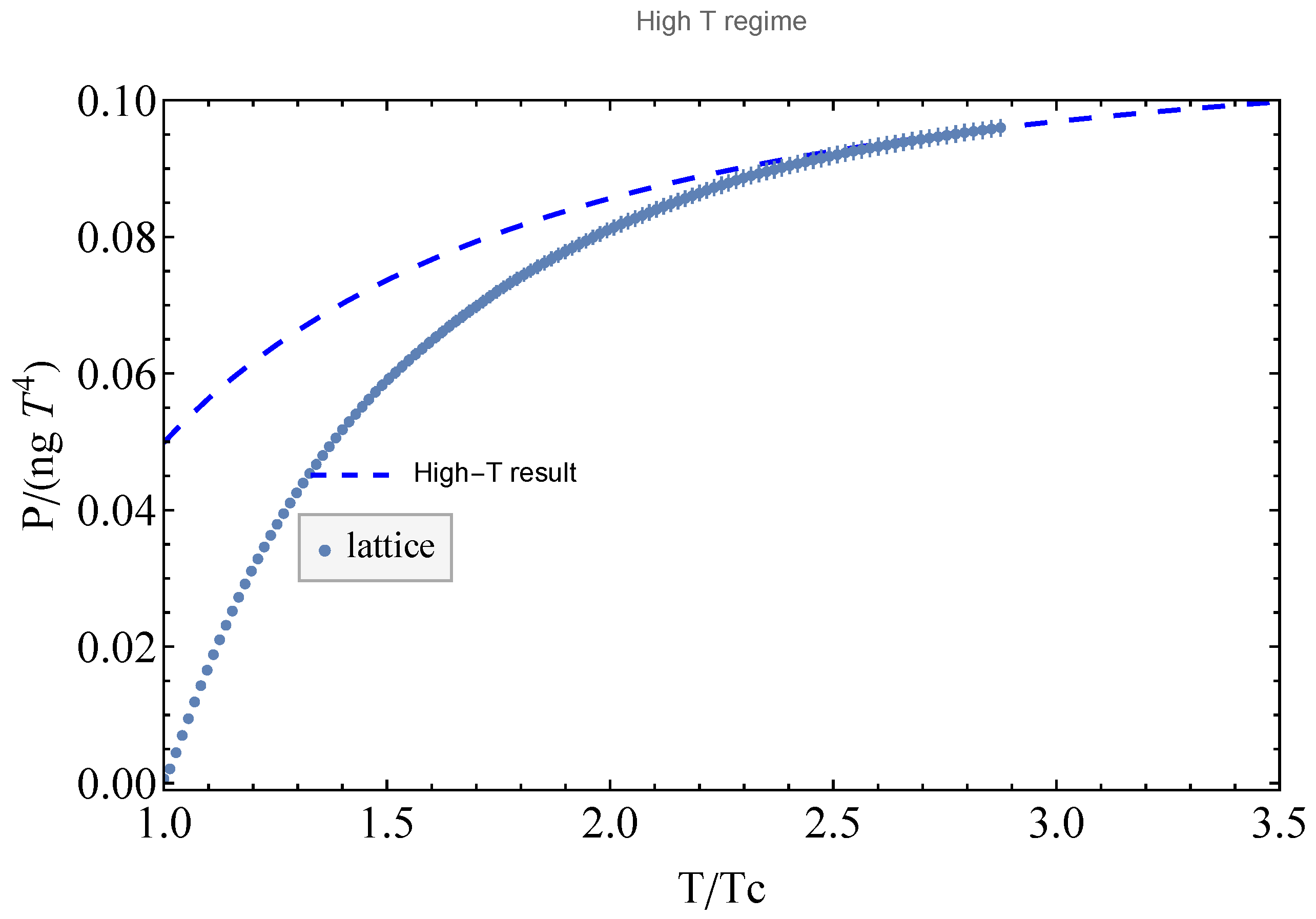
In the high-temperature regime, where perturbative QCD can be satisfactorily applied [21], we achieve the somewhat surprising result that the corresponding thermal series for a scalar field seems to fit very well to the results, mostly for the case of the energy density. We would like to emphasize that the fits we obtain in this regime cannot be successful for the same values of the ratio . The reason is that we are just extending our approach with a spectrum of massive glue particles to a regime with massless gluons. In addition, the glueball mass can entail some dependence on the temperature that we are not able to catch at this stage [22]. The achievement of satisfactory results, in the high-temperature limit (i.e., for small values of ) too, warrants some extended discussion. For this we consider the expansion
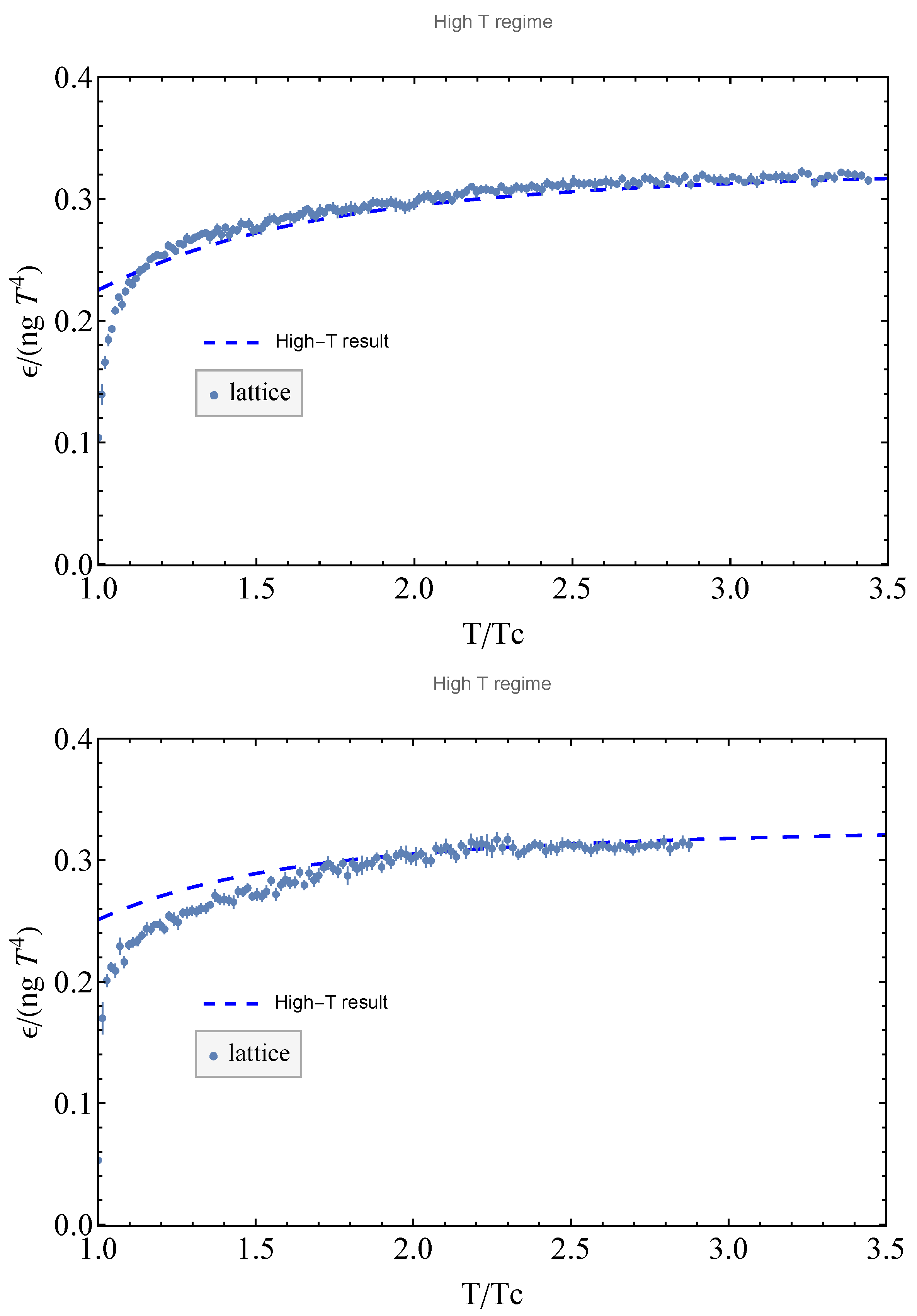
where is the Euler–Mascheroni constant. This corresponds to considering Equation (29) for only a single term and expanding for high temperatures for . The corresponding plots are given in Figure 3 and Figure 4. From these plots, it can be easily observed how harsh our approximation is compared to standard perturbative computation. Nevertheless, for the energy density in the high-temperature regime, we obtain Figure 4. The agreement in this case is excellent with the rule for the ratio and the number of colors satisfied again.

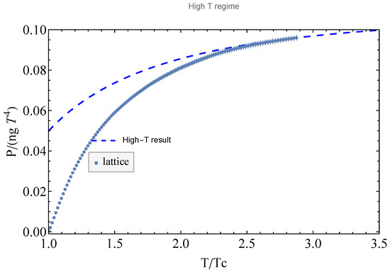
Figure 3.
Upper: Plot of the pressure p for in the high-temperature limit with the fitted ratio compared to the lattice data. Lower: The same for with the fitted ratio .
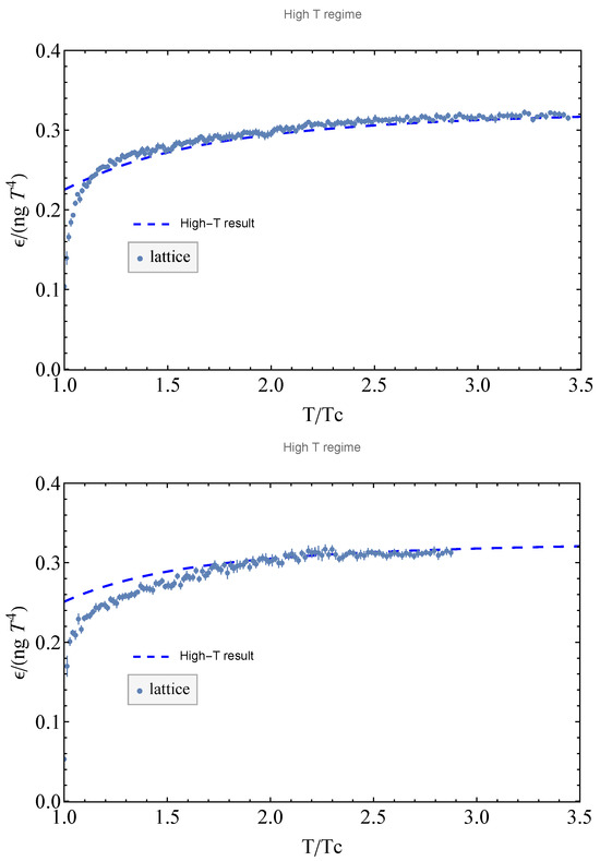
Figure 4.
Upper: Plot of the energy density for with the fitted ratio , as compared to the lattice data. Right: The same for with the fitted ratio .
We have fitted each quantity separately, as we cannot expect that the ratio will stay the same, and for consistency reasons. For the high-temperature limit, the ratio for the energy density is somewhat distant from the one for the pressure for . Overall, the agreement is excellent for a single fit parameter. Taking into account that we are working with asymptotic series with zero radius of convergence, we seem to have evaluated the optimal number of terms for a satisfactory agreement with lattice data.
6. Discussion and Conclusions
In this work, we have presented the non-perturbative partition function of the thermal Yang–Mills theory in the framework of Dyson–Schwinger equations with a non-trivial ground state in analytic form. Utilizing a novel technique for solving these equation in a differential form, we find very good consistency for the resulting thermodynamical observables—pressure and energy density—with the corresponding lattice results available for and colors. Our analytical approach provides a pathway for obtaining thermodynamic characteristics in terms of input parameters to a given action of the Yang–Mills theory. Indeed, in the considered IR limit of the theory, we show that the functional series for the partition function, already truncated at the quadratic term, shows good agreement between our results and the lattice data at low temperatures. While a standard technique could be applied for high temperatures, we considered the solution for the scalar field and found very good agreement for the energy density.
As the quadratic approximation already captures the most essential features of non-perturbative Yang–Mills dynamics at low temperatures, we believe that, with a complete evaluation of the partition function going beyond the quadratic order and accounting for higher-order correlation functions, a more precise behavior could be found, possibly with evidence for a smooth transition from a low-energy spectrum with glue states to that of a pure massless gluon spectrum, as observed in the asymptotic freedom regime.
A scenario with a spectrum of massive glue state excitations in a thermal setting for the Yang–Mills theory, starting from the available lattice data, has already been devised in the literature [23,24]. In our study, we demonstrate that the same behavior can be obtained analytically.
Cosmological first-order phase transitions (FOPT) in the early universe are known to radiate gravitational waves (GWs), which are potentially detectable in upcoming GW missions like LISA [25,26,27,28]. If such a signal were to be detected, this would inevitable give hints for new physics, since the electroweak and QCD phase transitions in the standard model are known as cross-overs, not as FOPT. Consequently, studying such GW signals could allow us to probe the dynamics of otherwise completely inaccessible dark or hidden sectors [29,30,31]. Therefore, we envisage a possible application of our approach to studies of such phase transitions in the early universe, particularly for strong coupling. Yang–Mills theories, featuring color confinement string FOPTs [3,32], naturally appear in several well-motivated viable extensions of the standard model; see studies in Refs. [33,34,35,36,37,38,39,40,41]. Since the only free and independent parameter here is the confinement scale, these scenarios can be deemed minimal, thus serving as suitable benchmark models. Previous attempts to study the GW signal in such models in Refs. [42,43,44,45,46,47,48,49] suffer from uncertainties related to non-perturbative effects, or rely on lattice calculations or methods like AdS/CFT [50] due to the strong coupling involved. We envisage the method developed in this paper to make quantitative estimates for such scenarios. As this is beyond the scope of the present paper, we plan to take up this subject in a future publication, given the timeline of the LISA experiment that is coming very soon and LiGO already taking data at present.
Our results are expected to also have a strong impact on a possible resolution of the long-standing problem of deriving the QCD equation of the state and the precise reconstruction of the QCD phase diagram, critical for many ongoing studies in particle physics (e.g., physics of the quark–gluon plasma) and astrophysics (e.g., the dynamics of neutron stars), and other issues in cosmology (e.g., dark matter, dark energy, and inflation); see Refs. [51,52,53].
Author Contributions
Conceptualization, M.F. and A.G.; methodology, M.F., A.G. and S.G.; software, M.F. and A.G.; validation, M.F., A.G. and S.G.; formal analysis, M.F. and A.G.; investigation, M.F. and A.G.; resources, M.F. and A.G.; data curation, M.F.; writing—original draft preparation, M.F.; writing—review and editing, S.G.; visualization, M.F.; supervision, M.F. and S.G.; project administration. All authors have read and agreed to the published version of the manuscript.
Funding
This research received no external funding.
Data Availability Statement
Data are contained within the article.
Acknowledgments
The authors thank Marco Panero for providing the data of the lattice computations for the purpose of comparison. We are also grateful to Roman Pasechnik and Zhi-Wei Wang who were greatly helpful during the first stage of this project.
Conflicts of Interest
The authors declare no conflicts of interest.
Appendix A. Two-Point Correlation Function and Spectrum
We have to solve the set of Dyson–Schwinger Equation (11); cf. Refs. [5,6,7,8]. The aim is to obtain a Fubini–Lipatov solution to represent the vacuum of the theory and a translation invariant two-point correlation function. Actually, both the equations can be solved analytically using Jacobi elliptic functions [54,55]. In physics, elliptic integrals and functions appear, for instance, for the exact solution of the physical pendulum, in the small angle approximation limited by the mathematical pendulum that obeys a linear differential equation. Without going into too much detail, the period of a physical pendulum is expressed in terms of the incomplete elliptic integral
with parameter , where the complete elliptic integral given by . The Jacobi elliptic functions are defined via this incomplete elliptic integral by the inversion of the equation , in the sense that , , and . Using the Jacobi elliptic sine, we can write
where , and and are two integration constants. This function is a solution for the nonlinear differential equation shown in the first line of (11), provided the dispersion relation
holds. It is interesting to point out that also solves the first equation in (11). Therefore, to choose one or the other solution spontaneously breaks the symmetry. Similarly, one can show that the two-point correlation function can be written in the form
where , with being the complete elliptic integral of the first kind. The technique is shown in Ref. [14] for the classical case but also applies straightforwardly here. The mass spectrum is
In order to go back to Equation (16), we set . In this case we obtain and . Inserting this back into Equation (A4), we are able to obtain the coefficients given in the main text.
Appendix B. One-Point Correlation Function
In taking instead of , Equation (7) for maps the classical equation of motion very well, given by
once we select the Feynman gauge [5]. However, there is an important difference as follows: Equation (7) contains a quantum correction of the form . After regularizing the divergences, this correction can have the effect of a small shift in the spectrum of the theory [7] that can be neglected. Our aim is to show how the Jacobi elliptic functions are suited to this equation. By taking the mixed symbols, in the simple case of ( is the group index), in the form
and using the mapping theorem between a scalar field and the Yang–Mills field [16,17],
solves
that is the first of Equation (11) for when the quantum corrections are neglected. Considering a solution of the form , we obtain
Therefore,
Using the identity [56], Equation (A9) is solved, provided the dispersion relation for holds. If the quantum corrections are neglected, we then obtain
that is Equation (13).
Appendix C. Evaluation of the Partition Function
Noting that the exponential function grants convergence for , one can expand
Because of the convergence of this series, one can freely interchange the integration and summation to obtain
The integral term can be rewritten in a known form via the change of variables . This yields (see Ref. [57], 3.389.4)
where is a modified Bessel function of the second kind. This yields Equation (29) in the main text. In physics, Bessel functions describe the vibration modes of a circular membrane, being solutions to the Bessel differential equation . Modified Bessel functions are those that obey the modified Bessel differential equation . An integral representation of the modified Bessel function of the second kind (diverging at the origin) is given by
References
- Pisarski, R. Quark gluon plasma as a condensate of SU(3) Wilson lines. Phys. Rev. D 2000, 62, 111501. [Google Scholar] [CrossRef]
- Sannino, F. Polyakov loops versus hadronic states. Phys. Rev. D 2002, 66, 034013. [Google Scholar] [CrossRef]
- Panero, M. Thermodynamics of the QCD plasma and the large-N limit. Phys. Rev. Lett. 2009, 103, 232001. [Google Scholar] [CrossRef] [PubMed]
- Carenza, P.; Pasechnik, R.; Salinas, G.; Wang, Z. Glueball Dark Matter Revisited. Phys. Rev. Lett. 2022, 129, 261302. [Google Scholar] [CrossRef] [PubMed]
- Frasca, M. Quantum Yang–Mills field theory. Eur. Phys. J. Plus 2017, 132, 38, Erratum in Eur. Phys. J. Plus 2017, 132, 242. [Google Scholar] [CrossRef]
- Frasca, M. Confinement in a three-dimensional Yang–Mills theory. Eur. Phys. J. C 2017, 77, 255. [Google Scholar] [CrossRef]
- Frasca, M. Spectrum of Yang–Mills theory in 3 and 4 dimensions. Nucl. Part. Phys. Proc. 2018, 294–296, 124–128. [Google Scholar] [CrossRef]
- Chaichian, M.; Frasca, M. Condition for confinement in non-Abelian gauge theories. Phys. Lett. B 2018, 781, 33–39. [Google Scholar] [CrossRef]
- Koberinski, A. Mathematical developments in the rise of Yang–Mills gauge theories. Synthese 2021, 198 (Suppl. S16), 3747–3777. [Google Scholar]
- Brink, L.; Phua, K.K. (Eds.) Proceedings of the Conference on 60 Years of Yang–Mills Gauge Field Theories: C.N. Yang’s Contributions to Physics, Nanyang Technological University, Singapore, 25–28 May 2015; World Scientific Publishing Co. Pte Ltd.: Singapore, 2016. [Google Scholar]
- Silva, J.; Khanna, F.; Matos Neto, A.; Santana, A. Generalized Bogolyubov transformation for confined fields: Applications in Casimir effect. Phys. Rev. A 2002, 66, 052101. [Google Scholar] [CrossRef]
- Santos, A.; Khanna, F. Casimir effect and Stefan–Boltzmann law in Yang–Mills theory at finite temperature. Int. J. Mod. Phys. A 2019, 34, 1950128. [Google Scholar] [CrossRef]
- Trotti, E.; Jafarzade, S.; Giacosa, F. Thermodynamics of the glueball resonance gas. Eur. Phys. J. C 2023, 83, 390. [Google Scholar] [CrossRef]
- Frasca, M.; Groote, S. Exact solutions to non-linear classical field theories. Symmetry 2024, 16, 1504. [Google Scholar] [CrossRef]
- Böhm, M.; Denner, A.; Joos, H. Gauge Theories of the Strong and Electroweak Interaction; B.G. Teubner: Stuttgart, Germany, 2001. [Google Scholar]
- Frasca, M. Infrared Gluon and Ghost Propagators. Phys. Lett. B 2008, 670, 73–77. [Google Scholar] [CrossRef]
- Frasca, M. Mapping a massless scalar field theory on a Yang–Mills theory: Classical case. Mod. Phys. Lett. A 2009, 24, 2425–2432. [Google Scholar] [CrossRef]
- Frasca, M.; Ghoshal, A.; Groote, S. Nambu–Jona-Lasinio model correlation functions from QCD. Nucl. Part. Phys. Proc. 2022, 318–323, 138–141. [Google Scholar] [CrossRef]
- Le Bellac, M. Thermal Field Theory; Cambridge University Press: Cambridge, UK, 2008. [Google Scholar]
- Lucini, B.; Panero, M. SU(N) gauge theories at large N. Phys. Rept. 2013, 526, 93–163. [Google Scholar] [CrossRef]
- Borsanyi, S.; Endrodi, G.; Fodor, Z.; Katz, S.; Szabo, K. Precision SU(3) lattice thermodynamics for a large temperature range. J. High Energy Phys. 2012, 7, 56. [Google Scholar] [CrossRef]
- Silva, P.J.; Oliveira, O.; Bicudo, P.; Cardoso, N. Gluon screening mass at finite temperature from the Landau gauge gluon propagator in lattice QCD. Phys. Rev. D 2014, 89, 074503. [Google Scholar] [CrossRef]
- Peshier, A.; Kampfer, B.; Pavlenko, O.; Soff, G. A Massive quasiparticle model of the SU(3) gluon plasma. Phys. Rev. D 1996, 54, 2399–2402. [Google Scholar] [CrossRef]
- Castorina, P.; Greco, V.; Jaccarino, D.; Zappalà, D. A Reanalysis of Finite Temperature SU(N) Gauge Theory. Eur. Phys. J. C 2011, 71, 1826. [Google Scholar] [CrossRef]
- Auclair, P.; Bacon, D.; Baker, T.; Barreiro, T.; Bartolo, N.; Belgacem, E.; Bellomo, N.; Ben-Dayan, I.; Bertacca, D.; Besancon, M.; et al. Cosmology with the Laser Interferometer Space Antenna. Living Rev. Rel. 2023, 26, 5. [Google Scholar]
- Amaro-Seoane, P.; Audley, H.; Babak, S.; Baker, J.; Barausse, E.; Bender, P.; Berti, E.; Binetruy, P.; Born, M.; Bortoluzzi, D.; et al. Laser Interferometer Space Antenna. arXiv 2017, arXiv:1702.00786. [Google Scholar]
- Janssen, G.; Hobbs, G.; McLaughlin, M.; Bassa, C.G.; Deller, A.T.; Kramer, M.; Hobbs, G.; McLaughlin, M.; Bassa, C.G.; Deller, A.T.; et al. Gravitational wave astronomy with the SKA. Proc. Sci. 2015, AASKA14, 37. [Google Scholar]
- Yagi, K.; Seto, N. Detector configuration of DECIGO/BBO and identification of cosmological neutron-star binaries. Phys. Rev. D 2011, 83, 044011, Erratum in Phys. Rev. D 2017, 95, 109901. [Google Scholar]
- Schwaller, P. Gravitational Waves from a Dark Phase Transition. Phys. Rev. Lett. 2015, 115, 181101. [Google Scholar] [CrossRef]
- Breitbach, M.; Kopp, J.; Madge, E.; Opferkuch, T.; Schwaller, P. Dark, Cold, and Noisy: Constraining Secluded Hidden Sectors with Gravitational Waves. J. Cosmol. Astropart. Phys. 2019, 7, 7. [Google Scholar] [CrossRef]
- Fairbairn, M.; Hardy, E.; Wickens, A. Hearing without seeing: Gravitational waves from hot and cold hidden sectors. J. High Energy Phys. 2019, 7, 44. [Google Scholar]
- Svetitsky, B.; Yaffe, L.G. Critical Behavior at Finite Temperature Confinement Transitions. Nucl. Phys. B 1982, 210, 423–447. [Google Scholar]
- Gross, D.J.; Harvey, J.A.; Martinec, E.J.; Rohm, R. The Heterotic String. Phys. Rev. Lett. 1985, 54, 502–505. [Google Scholar]
- Dixon, L.J.; Harvey, J.A.; Vafa, C.; Witten, E. Strings on Orbifolds. Nucl. Phys. B 1985, 261, 678–686. [Google Scholar]
- Dixon, L.J.; Harvey, J.A.; Vafa, C.; Witten, E. Strings on Orbifolds. 2. Nucl. Phys. B 1986, 274, 285–314. [Google Scholar] [CrossRef]
- Acharya, B.S. M theory, Joyce orbifolds and super Yang–Mills. Adv. Theor. Math. Phys. 1999, 3, 227–248. [Google Scholar] [CrossRef]
- Halverson, J.; Morrison, D.R. On gauge enhancement and singular limits in G2 compactifications of M-theory. J. High Energy Phys. 2016, 4, 100. [Google Scholar]
- Asadi, P.; Kramer, E.D.; Kuflik, E.; Ridgway, G.W.; Slatyer, T.R.; Smirnov, J. Thermal squeezeout of dark matter. Phys. Rev. D 2021, 104, 095013. [Google Scholar] [CrossRef]
- Asadi, P.; Kramer, E.D.; Kuflik, E.; Ridgway, G.W.; Slatyer, T.R.; Smirnov, J. Accidentally Asymmetric Dark Matter. Phys. Rev. Lett. 2021, 127, 211101. [Google Scholar] [CrossRef] [PubMed]
- Bai, Y.; Schwaller, P. Scale of dark QCD. Phys. Rev. D 2014, 89, 063522. [Google Scholar] [CrossRef]
- Schwaller, P.; Stolarski, D.; Weiler, A. Emerging Jets. J. High Energy Phys. 2015, 5, 59. [Google Scholar] [CrossRef]
- Halverson, J.; Long, C.; Maiti, A.; Nelson, B.; Salinas, G. Gravitational waves from dark Yang–Mills sectors. J. High Energy Phys. 2021, 5, 154. [Google Scholar] [CrossRef]
- Bigazzi, F.; Caddeo, A.; Cotrone, A.L.; Paredes, A. Fate of false vacua in holographic first-order phase transitions. J. High Energy Phys. 2020, 12, 200. [Google Scholar] [CrossRef]
- Bigazzi, F.; Caddeo, A.; Cotrone, A.L.; Paredes, A. Dark Holograms and Gravitational Waves. J. High Energy Phys. 2021, 4, 94. [Google Scholar] [CrossRef]
- Huang, W.C.; Reichert, M.; Sannino, F.; Wang, Z.W. Testing the dark SU(N) Yang–Mills theory confined landscape: From the lattice to gravitational waves. Phys. Rev. D 2021, 104, 035005. [Google Scholar] [CrossRef]
- Wang, X.; Huang, F.P.; Zhang, X. Bubble wall velocity beyond leading-log approximation in electroweak phase transition. arXiv 2011, arXiv:2011.12903. [Google Scholar]
- Kang, Z.; Zhu, J.; Matsuzaki, S. Dark confinement-deconfinement phase transition: A roadmap from Polyakov loop models to gravitational waves. J. High Energy Phys. 2021, 9, 60. [Google Scholar]
- Yamada, M.; Yonekura, K. Cosmic F- and D-strings from pure Yang–Mills theory. Phys. Lett. B 2023, 838, 137724. [Google Scholar]
- Yamada, M.; Yonekura, K. Cosmic strings from pure Yang–Mills theory. Phys. Rev. D 2022, 106, 123515. [Google Scholar] [CrossRef]
- Morgante, E.; Ramberg, N.; Schwaller, P. Gravitational waves from dark SU(3) Yang–Mills theory. Phys. Rev. D 2023, 107, 036010. [Google Scholar] [CrossRef]
- Hindmarsh, M.; Philipsen, O. WIMP dark matter and the QCD equation of state. Phys. Rev. D 2005, 71, 087302. [Google Scholar] [CrossRef]
- Drees, M.; Hajkarim, F.; Schmitz, E. The Effects of QCD Equation of State on the Relic Density of WIMP Dark Matter. J. Cosmol. Astropart. Phys. 2015, 6, 25. [Google Scholar]
- Hajkarim, F.; Schaffner-Bielich, J.; Wystub, S.; Wygas, M. Effects of the QCD equation of state and lepton asymmetry on primordial gravitational waves. Phys. Rev. D 2019, 99, 103527. [Google Scholar]
- Bateman, H. Higher Transcendental Functions [Volumes I–III]; Bateman Manuscript Project; McGraw-Hill Book Company: New York, NY, USA, 1953. [Google Scholar]
- Whittaker, E.T.; Watson, G.N. A Course of Modern Analysis, 4th ed.; Cambridge University Press: Cambridge, UK, 1927. [Google Scholar]
- [DLMF]. NIST Digital Library of Mathematical Functions; Olver, F.W.J., Olde Daalhuis, A.B., Lozier, D.W., Schneider, B.I., Boisvert, R.F., Clark, C.W., Miller, B.R., Saunders, B.V., Cohl, H.S., McClain, M.A., Eds.; Release 1.1.6 of 2022-06-30. Available online: https://dlmf.nist.gov/ (accessed on 23 March 2025).
- Gradshteyn, I.S.; Ryzhik, I.M. Table of Integrals, Series, and Products, 7th ed.; Translated from the Russian; Jeffrey, A.; Zwillinger, D., Translators; Elsevier; Academic Press: Amsterdam, The Netherlands, 2007; p. xlviii+1171, ISBNs: 978-0-12-373637-6; 0-12-373637-4. [Google Scholar]
Disclaimer/Publisher’s Note: The statements, opinions and data contained in all publications are solely those of the individual author(s) and contributor(s) and not of MDPI and/or the editor(s). MDPI and/or the editor(s) disclaim responsibility for any injury to people or property resulting from any ideas, methods, instructions or products referred to in the content. |
© 2025 by the authors. Licensee MDPI, Basel, Switzerland. This article is an open access article distributed under the terms and conditions of the Creative Commons Attribution (CC BY) license (https://creativecommons.org/licenses/by/4.0/).