Fractional Landweber Regularization Method for Identifying the Source Term of the Time Fractional Diffusion-Wave Equation

Abstract

In this paper, the inverse problem of identifying the source term of the time fractional diffusion-wave equation is studied. This problem is ill-posed, i.e., the solution (if it exists) does not depend on the measurable data. Under the priori bound condition, the condition stable result and the optimal error bound are all obtained. The fractional Landweber iterative regularization method is used to solve this inverse problem. Based on the priori regularization parameter selection rule and the posteriori regularization parameter selection rule, the error estimation between the regularization solution and the exact solution is obtained. Moreover, the error estimations are all order optimal. At the end, three numerical examples are given to prove the effectiveness and stability of this regularization method.

1. Introduction

In this paper, the problem of identifying the source term of the time fractional diffusion-wave equation is considered. The following time fractional diffusion-wave equation is studied:

$$\left\{\begin{array}{cc}{D}_t^{\alpha }u(x,t)=u_{xx}(x,t)+f\left(x\right),\hfill & (x,t)\in \overline{\Omega }\times [0,T],1<\alpha \le 2,\hfill \\ u(x,t)=0,\hfill & x\in \partial \Omega ,\hfill \\ u(x,0)=\varphi \left(x\right),\hfill & x\in \Omega ,\hfill \\ u_t(x,0)=\psi \left(x\right),\hfill & x\in \Omega ,\hfill \\ u(x,T)=g\left(x\right),\hfill & x\in \Omega ,\hfill \end{array}\right.$$

(1)

where $D_t^{\alpha }$ is the Caputo fractional derivative of order $\alpha (1<\alpha \le 2)$, which is defined as follows

$$D_t^{\alpha }u(x,t)={\displaystyle \frac{1}{\Gamma (2-\alpha )}}{\int }_a^t{\displaystyle \frac{{\partial }^{2}u(x,s)}{\partial s^2}}{\displaystyle \frac{ds}{{(t-s)}^{\alpha -1}}},1<\alpha \le 2,$$

where $\Gamma (·)$ is a gamma function and $\Omega$ is a bounded domain with a sufficiently smooth boundary. The Caputo derivative is a definition of a fractional derivative that is particularly useful in solving fractional differential equations with physically interpretable initial conditions. Unlike the Riemann–Liouville fractional derivative, the Caputo derivative allows initial conditions to be expressed in terms of standard integer-order derivatives, making it more suitable for modeling real-world problems. The Caputo fractional derivative has power-law decay properties, which can naturally describe the historical dependence and long-term memory effects of the system; for example, in viscoelastic materials, the influence of historical deformation on the current state during the stress relaxation process of materials (integer-order derivatives can only describe instantaneous response). In abnormal diffusion, Caputo fractional order equations can describe super-diffusion or sub-diffusion.

There are some other fractional derivative:

(1)

Riemann–Liouville derivative [1]:

$$D_{a+}^{\alpha }u(x,t)={\displaystyle \frac{1}{\Gamma (n-\alpha )}}{\left({\displaystyle \frac{d}{dt}}\right)}^n{\int }_a^t{\displaystyle \frac{f\left(\tau \right)}{{(t-\tau )}^{\alpha -n+1}}}d\tau ,$$

where $\Gamma (·)$ is a gamma function and a is the lower limit of integration (often $a=0$, $n=\left[a\right]$ (the smallest integer $\ge a$)). Unlike integer-order derivatives, the Riemann–Liouville derivative depends on the entire history of $f\left(t\right)$ from a to t.

(2)

Caputo–Hadamard fractional derivative [2,3]:

$${}_{CH}D_{a,t}^{\alpha }u(x,t)={\displaystyle \frac{1}{\Gamma (1-\alpha )}}{\int }_a^t{(log{\displaystyle \frac{t}{w}})}^{-\alpha }\delta u(x,w)dw,0<\alpha <1,$$

where $\delta =t{\displaystyle \frac{d}{dt}}$, $\Gamma \left(x\right)$ is a Gamma function. The Caputo–Hadamard fractional derivative is particularly useful for modeling systems with geometric or multiplicative memory effects.

(3)

Caputo–Fabrizio fractional derivative [4]:

$${}_{CF}D_{0,t}^{\alpha }\nu \left(t\right)={\displaystyle \frac{1}{1-\alpha }}{\int }_0^{t}exp(-{\displaystyle \frac{\alpha }{1-\alpha }}(t-z)){\displaystyle \frac{\partial \nu \left(z\right)}{\partial z}}dz,fort\ge 0.$$

Fractional models have become practically necessary in various fields due to their ability to capture complex phenomena that traditional integer-order models cannot adequately describe. Here is a structured summary of the key reasons:

1.

Memory and non-local effects: fractional derivatives inherently account for memory and history dependence, which is crucial in materials science (e.g., viscoelasticity) and processes with long-range temporal correlations. Integer-order models require additional terms or integrals to approximate such effects, increasing complexity.

2.

Anomalous diffusion: in systems like biological tissues or porous media, diffusion often follows a power-law rather than linear growth (as in Fick’s law). Fractional diffusion equations directly model such sub-diffusion or super-diffusion, whereas integer-order models fail to capture these dynamics without unrealistic assumptions.

3.

Power-law dynamics: natural systems frequently exhibit power-law relaxation or frequency responses (e.g., electrochemical impedance, viscoelastic damping). Fractional models naturally describe these behaviors, avoiding the need for infinite exponential terms in integer-order frameworks.

4.

Parsimonious representation: fractional models often require fewer parameters to describe complex behavior. For example, a single fractional-order term can replace multiple integer-order terms, simplifying control systems and reducing computational overhead.

5.

Non-locality in space and time: fractional operators are non-local, making them suitable for phenomena with spatial or temporal long-range interactions. Integer-order models would need ad hoc modifications to incorporate such effects.

6.

Improved data fitting and prediction: experimental data with power-law decay or non-exponential relaxation (e.g., drug transport in tissues, financial time series) often align better with fractional models, yielding lower fitting errors and more accurate predictions.

7.

Robust control systems: fractional-order controllers provide enhanced robustness and tuning flexibility compared traditional PID controllers, particularly for systems with uncertain or complex dynamics.

• Limitations of integer-order models:

1.

Inability to inherently model memory or history-dependent processes.

2.

Require higher-order terms or complex systems to approximate fractional behavior.

3.

Fail to capture power-law dynamics and anomalous diffusion without oversimplification.

While integer-order models remain sufficient for many well-understood systems, fractional models are indispensable in scenarios involving memory, non-locality, power-law responses, or anomalous diffusion. Their practical necessity arises from their accuracy, efficiency, and alignment with observed natural and engineered systems, despite the computational challenges they may pose.

Selecting fractional orders in real-world applications requires a systematic approach that balances theoretical insights, empirical data, and practical constraints. Below are the key guidelines organized for clarity:

1.

Understand the system’s physical/behavioral basis: for systems exhibiting properties between two states (e.g., viscoelastic materials between solid and fluid), choose orders closer to 0 (viscous) or 1 (elastic) based on dominance.

2.

Anomalous diffusion: in sub-diffusion (slower spread) or super-diffusion (faster spread), match the order to the diffusion exponent observed experimentally. Memory effects: lower orders (e.g., $0<\alpha <1$) is called sub-diffusion. $1<\alpha <2$ is called super-diffusion.

In Equation (1), the problem is a positive one when the source term, $f\left(x\right)$, initial value, $\varphi \left(x\right)$, and $\psi \left(x\right)$ are known. If the source term, $f\left(x\right)$, is unknown, use the additional data $u(x,T)=g\left(x\right)$ to identify the unknown source, $f\left(x\right)$. This is an inverse problem. In addition, it is assumed that the exact data, $g\left(x\right)$, with the measured data, $g^{\delta }\left(x\right)$, satisfy the following noise assumption

$$\parallel g^{\delta }\left(x\right)-g\left(x\right)\parallel \le \delta .$$

(2)

In other words, Formula (2) is also equivalent to

$$\parallel h^{\delta }\left(x\right)-h\left(x\right)\parallel \le \delta ,$$

(3)

where $h_n=g_n-E_{\alpha ,1}(-{\lambda }_n{T}^{\alpha }){\varphi }_n-T{E}_{\alpha ,2}(-{\lambda }_n{T}^{\alpha }){\psi }_n$, $\parallel ·\parallel$ is the $L^2(\Omega )$ norm and $\delta$ is the noise level.

In recent years, the time fractional diffusion equation has been studied by many mathematical researchers. As a generalization of the classical diffusion equation and the wave equation, we are not unfamiliar with it, and it can be applied to simulate actual diffusion and wave phenomena such as fluid flow and oil formation. There are many studies on the identification of the unknown term in the time fractional diffusion equation, and there are also studies on the simultaneous identification of two unknown terms in the time fractional diffusion equation, for example, the identification of unknown items such as the initial value, the source term, and the fractional order. In Ref. [5], the classical Tikhonov regularization method and the simplified Tikhonov regularization method are used to solve the inverse problem of space-dependent sources in the time fractional diffusion equation, and a series of studies are carried out. In Ref. [6], the authors consider the inverse problem of simultaneous inversion of the source term and initial value of the time fractional diffusion equation based on the Fourier method, and give error estimations under the selection rules of the priori and posteriori regularization parameters. In Ref. [7], the authors derive the construction of the solution of the inverse problem by using the Landweber iterative method of the corresponding conjugate operator equation of the first type of operator equation based on the Fourier method, and give the priori and posteriori error estimations by selecting the appropriate regularization parameter. There are few studies on the identification of the unknown terms in the time fractional diffusion-wave equation, but more studies on its numerical methods. In Ref. [8], the authors develop two finite difference methods for the time fractional sub-diffusion equation with Dirichlet boundary conditions, in which the time direction is approximated by the fractional linear multi-step method and the spatial direction is approximated by the finite element method. In Ref. [9], the original problem is reduced to the initial boundary value problem on the bounded computational domain, which is equivalent to or approximate to the original problem by using the exact boundary condition or the approximate boundary condition on the artificial boundary, and the reduced problem on the bounded computational domain is solved by the finite difference method. In Ref. [10], the authors use the two-point gradient method to solve the zero-order coefficient inverse problem numerically and obtain some properties of the forward operator that guarantee the convergence of the algorithm.

With the promotion of the science and technology revitalization strategy, the limitations of many actual models describing natural phenomena do not meet the conditions of “correct models”, which is called an ill-posed problem. To recover the well-posedness of the inverse problem, the regularization method is mainly used. The basic idea of the regularization method is to redefine the concept of the solution of the ill-posed problem by using part of the additional information of the problem, and introduce the linear functional to give a stable method to approximate the solution of the original problem. In the process of solving the inverse problem, a variety of regularization methods have emerged, such as the Landweber iterative regularization method [11,12,13], Tikhonov regularization method [14], the quasi-boundary regularization method [15,16,17], the quasi-reversible regularization method [18], the truncated regularization method [19,20,21,22], the mollification method [23], the Fourier method [24], and so on.

The paper is structured as follows. In Section 2, some auxiliary lemmas, and the solution and conditional stability result of the source term, $f\left(x\right)$, are given. In Section 3, some basic theoretical knowledge and the optimal error bound of the inverse problem (1) are given. In Section 4, we apply the fractional Landweber iterative regularization method to solve the ill-posed problem (1) to recover its stability. In Section 5, we apply three numerical examples to verify the effectiveness and feasibility of the fractional Landweber iterative regularization method. And finally, a brief conclusion of the paper is given in Section 6.

2. Some Auxiliary Results and the Conditional Stability Result of the Problem (1)

In this section, all the work we do is to prepare for the subsequent application of regularization methods to recover the stability of Formula (1). The definition and some properties of the Mittag-Leffler function are given, and the exact solution of the source term, $f\left(x\right)$, in Equation (1) is obtained by a simple calculation. At the end, we give the conditional stability result of the source term in order to facilitate the calculation of the posteriori error estimation.

2.1. Some Auxiliary Results

In this part, we will introduce some significant lemmas and some properties of the Mittag-Leffler function needed to complete the paper.

Definition 1.

Suppose ${\lambda }_n$ and $X_n\left(x\right)$ are the Dirichlet eigenvalues and eigenfunctions of ${\displaystyle \frac{{\partial }^2}{\partial x^2}}$ on the domain Ω, they satisfy

$$\left\{\begin{array}{cc}-{\displaystyle \frac{{\partial }^2}{\partial x^2}}{X}_n\left(x\right)={\lambda }_n{X}_n\left(x\right),\hfill & x\in \Omega ,\hfill \\ X_n\left(x\right)=0,\hfill & x\in \partial \Omega ,\hfill \end{array}\right.$$

(4)

where $0<{\lambda }_1\le {\lambda }_2\le \cdots \le {\lambda }_n\le \cdots$, ${lim}_{n\to \infty }{\lambda }_n=+\infty$ and $X_n\left(x\right)\in H^2(\Omega )\bigcap H_0^1(\Omega )$. As we all know, ${\left\{X_n\left(x\right)\right\}}_{n=1}^{\infty }$ is an orthogonal basis in $L^2(\Omega )$.

Definition 2.

For any $p>0$, we define the following space

$$H^p(\Omega )=\left\{f\in L^2(\Omega )|\sum _{n=1}^{\infty }{\lambda }_n^p{\left|(f,X_n)\right|}^2<\infty \right\},$$

(5)

where $(·,·)$ represents the inner product in $L^2(\Omega )$, and $H^p(\Omega )$ is the Hilbert space with the norm

$${\parallel f(·)\parallel }_{H^p(\Omega )}:={\left(\sum _{n=1}^{\infty }{\lambda }_n^p{\left|(f,X_n)\right|}^2\right)}^{{\displaystyle \frac{1}{2}}}.$$

(6)

Definition 3

([1]). The Mittag-Leffler function is defined as follows

$$E_{\alpha ,\beta }\left(z\right)=\sum _{k=0}^{\infty }{\displaystyle \frac{z^k}{\Gamma (\alpha k+\beta )}},z\in C,$$

(7)

where $\alpha >0$ and $\beta \in R$ are arbitrary constants.

Lemma 1

([1]). If $\lambda >0$, the following equation holds

$${\int }_0^{\infty }{e}^{-pt}{t}^{\alpha m+\beta -1}{E}_{\alpha ,\beta }^{\left(m\right)}(\pm a{t}^{\alpha })dt={\displaystyle \frac{m!p^{\alpha -\beta }}{{(p^{\alpha }\mp a)}^{m+1}}},Re\left(p\right)>{\left|a\right|}^{{\displaystyle \frac{1}{\alpha }}},$$

(8)

where $E_{\alpha ,\beta }^{\left(m\right)}\left(y\right):={\displaystyle \frac{d^m}{d{y}^m}}{E}_{\alpha ,\beta }\left(y\right)$.

Lemma 2

([25]). For the Mittag-Leffler function, we have the following properties

$$E_{\alpha ,\beta }\left(z\right)=z·E_{\alpha ,\alpha +\beta }\left(z\right)+{\displaystyle \frac{1}{\Gamma \left(\beta \right)}},$$

(9)

where $\alpha >0$ and $\beta \in R$ are arbitrary constants.

Lemma 3

([26]). For any $0<\alpha <1$ and $z\ge 0$, there is $0\le E_{\alpha ,1}(-z)\le 1$ and $E_{\alpha ,1}(-z)$ is a strictly decreasing function, that is,

$${(-1)}^n{\displaystyle \frac{d^{\alpha }}{d{z}^{\alpha }}}{E}_{\alpha ,1}(-z)\ge 0,z\ge 0.$$

(10)

Lemma 4.

Supposing that $p>0$, $0<\mu <1$, $T>0$, and $0<{\lambda }_1<{\lambda }_n$, the following inequality holds

$$r_1\left(s\right)={\displaystyle \frac{\mu s^{2-\frac{p}{2}}}{C_1^2+\mu s^2}}\le \left\{\begin{array}{ccc}{C}_6{\mu }^{{\displaystyle \frac{p}{4}}},\hfill & \hfill & 0<p<4,\hfill \\ C_7\mu ,\hfill & \hfill & p\ge 4,\hfill \end{array}\right.$$

(11)

where $s:={\lambda }_n$, $C_6:={\displaystyle \frac{1}{4}}{p}^{{\displaystyle \frac{p}{4}}}{C}_1^{-{\displaystyle \frac{p}{2}}}{(4-p)}^{1-{\displaystyle \frac{p}{4}}}$, $C_7:={\displaystyle \frac{{\lambda }_1^{2-\frac{p}{2}}}{C_1^2}}$.

Proof. 

when $0<p<4$, $s_0$ satisfies $r_1^{\prime }\left(s_0\right)=0$, then we obtain

$$s_0={\left({\displaystyle \frac{(4-p)C_1^2}{p\mu }}\right)}^{{\displaystyle \frac{1}{2}}},$$

Thereby,

$$r_1\left(s\right)\le r_1\left(s_0\right)={\displaystyle \frac{\mu {\left({\left(\frac{(4-p)C_1^2}{p\mu }\right)}^{\frac{1}{2}}\right)}^{2-\frac{p}{2}}}{C_1^2+\mu \frac{(4-p)C_1^2}{p\mu }}}={\displaystyle \frac{1}{4}}{p}^{{\displaystyle \frac{p}{4}}}{C}_1^{-{\displaystyle \frac{p}{2}}}{(4-p)}^{1-{\displaystyle \frac{p}{4}}}{\mu }^{{\displaystyle \frac{p}{4}}}=C_6{\mu }^{{\displaystyle \frac{p}{4}}},$$

when $p\ge 4$, we obtain

$$r_1\left(s\right)={\displaystyle \frac{\mu s^{2-\frac{p}{2}}}{C_1^2+\mu s^2}}\le {\displaystyle \frac{{\lambda }_1^{2-\frac{p}{2}}}{C_1^2}}\mu =C_7\mu .$$

□

Lemma 5.

Supposing that $p>0$, $0<\mu <1$, $T>0$, and $0<{\lambda }_1<{\lambda }_n$, the following inequality holds

$$r_2\left(s\right)={\displaystyle \frac{\mu s^{1-\frac{p}{2}}}{C_1^2+\mu s^2}}\le \left\{\begin{array}{ccc}{C}_8{\mu }^{{\displaystyle \frac{p+2}{4}}},\hfill & \hfill & 0<p<2,\hfill \\ C_9\mu ,\hfill & \hfill & p\ge 2,\hfill \end{array}\right.$$

(12)

where $s:={\lambda }_n$, $C_8:={\displaystyle \frac{1}{4}}{C}_1^{-{\displaystyle \frac{p+2}{2}}}{(2-p)}^{{\displaystyle \frac{2-p}{4}}}{(p+2)}^{{\displaystyle \frac{p+2}{4}}}$, $C_9:={\displaystyle \frac{{\lambda }_1^{1-\frac{p}{2}}}{C_1^2}}$.

Proof. 

when $p\ge 4$, $s_0$ satisfies $r_2^{\prime }\left(s_0\right)=0$, then we obtain

$$s_0={\left({\displaystyle \frac{(2-p)C_1^2}{(p+2)\mu }}\right)}^{{\displaystyle \frac{1}{2}}}.$$

Thereby,

$$r_2\left(s\right)\le r_2\left(s_0\right)={\displaystyle \frac{\mu {\left({\left(\frac{(2-p)C_1^2}{(p+2)\mu }\right)}^{\frac{1}{2}}\right)}^{1-\frac{p}{2}}}{C_1^2+\mu \frac{(2-p)C_1^2}{(p+2)\mu }}}={\displaystyle \frac{1}{4}}{C}_1^{-{\displaystyle \frac{p+2}{2}}}{(2-p)}^{{\displaystyle \frac{2-p}{4}}}{(p+2)}^{{\displaystyle \frac{p+2}{4}}}{\mu }^{{\displaystyle \frac{p+2}{4}}},$$

when $p\ge 2$, we obtain

$$r_2\left(s\right)={\displaystyle \frac{\mu s^{1-\frac{p}{2}}}{C_1^2+\mu s^2}}\le {\displaystyle \frac{{\lambda }_1^{1-\frac{p}{2}}}{C_1^2}}\mu .$$

□

2.2. Solution of the Problem (1)

In this part, we will give the exact solution of the problem (1) and analyze its ill-posedness. In addition, the conditional stability result is given, which will be used in the calculation of the posterior error estimation.

At the very beginning, using the method of separation of variables, Laplace transform and inverse Laplace transform, we obtain the solution of the problem (1)

$$u(x,t)=\sum _{n=1}^{\infty }\left(E_{\alpha ,1}(-{\lambda }_n{t}^{\alpha }){\varphi }_n+t{E}_{\alpha ,2}(-{\lambda }_n{t}^{\alpha }){\psi }_n+t^{\alpha }{E}_{\alpha ,\alpha +1}(-{\lambda }_n{t}^{\alpha })f_n\right)X_n\left(x\right),$$

(13)

where ${\varphi }_n:=(\varphi \left(x\right),X_n\left(x\right))$, ${\psi }_n:=(\psi \left(x\right),X_n\left(x\right))$, and $f_n:=(f\left(x\right),X_n\left(x\right))$ are the Fourier coefficients. According to Equation (13) and $u(x,T)=g\left(x\right)$, we obtain the source term, $f\left(x\right)$, as follows

$$f\left(x\right)=\sum _{n=1}^{\infty }{\displaystyle \frac{h_n}{{\lambda }_n^{-1}(1-E_{\alpha ,1}(-{\lambda }_n{T}^{\alpha }))}}{X}_n\left(x\right),$$

(14)

where $h_n=g_n-E_{\alpha ,1}(-{\lambda }_n{T}^{\alpha }){\varphi }_n-T{E}_{\alpha ,2}(-{\lambda }_n{T}^{\alpha }){\psi }_n$, $h_n=(h\left(x\right),X_n\left(x\right))$, and $g_n=(g\left(x\right),X_n\left(x\right))$ are the Fourier coefficients.

In order to solve the ill-posed problem (1) successfully, a linear self-adjoint operator $K:f(·)\to h(·)$ is defined. Of course, the problem (1) can be converted to the following operator equation: $Kf\left(x\right)=h\left(x\right)={\sum }_{n=1}^{\infty }{\lambda }_n^{-1}(1-E_{\alpha ,1}(-{\lambda }_n{T}^{\alpha }))f_n{X}_n\left(x\right)$. From the above equation, the singular value is $K_n:={\lambda }_n^{-1}(1-E_{\alpha ,1}(-{\lambda }_n{T}^{\alpha }))$ and its eigenfunction is $X_n\left(x\right)$.

When $n\to \infty$, ${\lambda }_n\to \infty$, $K_n\to \infty$, it can be seen from Formula (14) that a small error in $h\left(x\right)$ will cause a huge change in the source term, $f\left(x\right)$. Therefore, this is a typical ill-posed problem, which will be solved by the regularization method in this paper. Here, we give the prior bound as follows

$${\parallel f(·)\parallel }_{H^p(\Omega )}={\left(\sum _{n=1}^{\infty }{\lambda }_n^p{f}_n^2\right)}^{{\displaystyle \frac{1}{2}}}\le E,$$

(15)

where p and E are both constants.

2.3. The Conditional Stability Result of the Problem (1)

Theorem 1.

Suppose $f\left(x\right)$ satisfies the prior bound condition in Equation (15), then we obtain the conditional stability of the source term, $f\left(x\right)$, as follows

$$\parallel f(·)\parallel \le C_1^{-{\displaystyle \frac{p}{p+2}}}{E}^{{\displaystyle \frac{2}{p+2}}}{\parallel h\left(x\right)\parallel }^{{\displaystyle \frac{p}{p+2}}},p>0,$$

(16)

where $C_1:=1-E_{\alpha ,1}(-{\lambda }_1{T}^{\alpha }).$

Proof. 

By combining Formulas (14) and (15) and the Hölder inequality, we obtain

$$\begin{array}{cc}\hfill {\parallel f\left(x\right)\parallel }^2& =\parallel \sum _{n=1}^{\infty }{\displaystyle \frac{h_n}{{\lambda }_n^{-1}(1-E_{\alpha ,1}(-{\lambda }_n{T}^{\alpha }))}}{X}_n\left(x\right){\parallel }^2\hfill \\ & =\sum _{n=1}^{\infty }{\displaystyle \frac{h_n^2}{{\lambda }_n^{-2}{(1-E_{\alpha ,1}(-{\lambda }_n{T}^{\alpha }))}^2}}\hfill \\ & =\sum _{n=1}^{\infty }{\displaystyle \frac{h_n^{\frac{4}{p+2}}}{{\lambda }_n^{-2}{(1-E_{\alpha ,1}(-{\lambda }_n{T}^{\alpha }))}^2}}{h}_n^{{\displaystyle \frac{2p}{p+2}}}\hfill \\ & =\sum _{n=1}^{\infty }{\left({\displaystyle \frac{h_n^2}{{\left({\lambda }_n^{-1}(1-E_{\alpha ,1}(-{\lambda }_n{T}^{\alpha }))\right)}^{p+2}}}\right)}^{{\displaystyle \frac{2}{p+2}}}{\left(h_n^2\right)}^{{\displaystyle \frac{p}{p+2}}}\hfill \\ & \le {\left(\sum _{n=1}^{\infty }{\displaystyle \frac{h_n^2}{{\left({\lambda }_n^{-1}(1-E_{\alpha ,1}(-{\lambda }_n{T}^{\alpha }))\right)}^{p+2}}}\right)}^{{\displaystyle \frac{2}{p+2}}}{\left(\sum _{n=1}^{\infty }{h}_n^2\right)}^{{\displaystyle \frac{p}{p+2}}}\hfill \\ & ={\left(\sum _{n=1}^{\infty }{\lambda }_n^p{(1-E_{\alpha ,1}(-{\lambda }_n{T}^{\alpha }))}^{-p}{f}_n^2\right)}^{{\displaystyle \frac{2}{p+2}}}{\left(\sum _{n=1}^{\infty }{h}_n^2\right)}^{{\displaystyle \frac{p}{p+2}}}\hfill \\ & \le {\left(1-E_{\alpha ,1}(-{\lambda }_1{T}^{\alpha })\right)}^{-{\displaystyle \frac{2p}{p+2}}}{\left(\sum _{n=1}^{\infty }{\lambda }_n^p{f}_n^2\right)}^{{\displaystyle \frac{2}{p+2}}}{\left(\sum _{n=1}^{\infty }{h}_n^2\right)}^{{\displaystyle \frac{p}{p+2}}}\hfill \\ & \le {\left(1-E_{\alpha ,1}(-{\lambda }_1{T}^{\alpha })\right)}^{-{\displaystyle \frac{2p}{p+2}}}{E}^{{\displaystyle \frac{4}{p+2}}}{\parallel h\left(x\right)\parallel }^{{\displaystyle \frac{2p}{p+2}}}.\hfill \end{array}$$

Therefore,

$$\parallel f\left(x\right)\parallel \le {(1-E_{\alpha ,1}(-{\lambda }_1{T}^{\alpha }))}^{-{\displaystyle \frac{p}{p+2}}}{E}^{{\displaystyle \frac{2}{p+2}}}{\parallel h\left(x\right)\parallel }^{{\displaystyle \frac{p}{p+2}}}.$$

The proof of Theorem 1 is completed. □

3. Preliminary Results of the Problem (1) and Optimal Error Bound

3.1. Preliminary Results of the Problem (1)

Suppose K is a self-adjoint bounded and linear operator from X to Y, both X and Y are infinite-dimensional Hilbert space, and the range, $R\left(K\right)$, of the operator K is nonclosed. That is, the inverse problem represented by the following operator equation is ill-posed [27,28]

$$Kx=y,$$

(17)

where $x\in X$, $y\in Y$. The following noise assumption is satisfied between the measured data with error and the noisy data without error

$$\parallel y-y^{\delta }\parallel \le \delta .$$

(18)

Suppose $R:Y\to X$ is an arbitrary mapping whose x is approximated by $y^{\delta }$. As we have seen, R is the worst-case error, which is defined as [28]

$$\Delta (\delta ,M,R):=sup\{\parallel R{y}^{\delta }-x\parallel |x\in M,y^{\delta }\in Y,\parallel Kx-y^{\delta }\parallel \le \delta \}.$$

(19)

It describes that method R may produce a large error when the solution, x, of Equation (17) is transformed in the set. Here the worst-case error for all $R:Y\to X$ is defined as the optimal error bound, that is,

$$\Delta (\delta ,M):=\underset{R}{inf}\Delta (\delta ,M,R).$$

(20)

For the method $R_0$, the optimal and order optimal are defined as follows [27]

(i).

Optimal if $\Delta (\delta ,M,R_0)=\Delta (\delta ,M)$;

(ii).

The order is optimal if $\Delta (\delta ,M,R_0)\le C\Delta (\delta ,M)$, where $C\ge 1$.

• According to [29], we obtain

$$\Delta (\delta ,M)\ge \omega (\delta ,M),$$

(21)

where $\omega (\delta ,M)$, the modulus of the continuous operator $K^{-1}$, it is defined as follows

$$\omega (\delta ,M):=sup\{\parallel x_1-x_2\parallel |x_1,x_2\in M,\parallel K{x}_1-K{x}_2\parallel \le \delta \}.$$

(22)

As we know, the elements of M satisfy a certain source condition

$$M_{\phi ,E}=\{x\in X|x={\left[\phi \left(K^{*}K\right)\right]}^{{\displaystyle \frac{1}{2}}}v,\parallel v\parallel \le E\}.$$

(23)

The operator function $\phi \left(K^{*}K\right)$ is defined by the following spectral representation [29,30]

$$\phi \left(K^{*}K\right)={\int }_0^a\phi \left(\lambda \right)d{E}_{\lambda },$$

(24)

where $E_{\lambda }$ represents the spectral family of the operator function $K^{*}K$, a is a constant that satisfies $\parallel K^{*}K\parallel \le a$, $\phi \in C\left(\sigma \left(K^{*}K\right)\right)$, and $\phi \left(0\right)=0$, $\sigma \left(K^{*}K\right)$ represents the spectrum of operator $K^{*}K$. Therefore, we obtain the lower bound of Equation (20) as follows [29]

$$\Delta (\delta ,M_{\phi ,E})=\omega (\delta ,M_{\phi ,E}).$$

(25)

Assumption 1

([29]). The function $\phi \left(\lambda \right)$ is a continuous function with the following properties

(i).

${lim}_{\lambda \to 0}\phi \left(\lambda \right)=0$;

(ii).

φ is a strictly monotonically increasing function on $(0,a]$;

(iii).

$\rho \left(\lambda \right)=\lambda {\phi }^{-1}\left(\lambda \right):(0,\phi \left(a\right)]\to (0,a\phi \left(a\right)]$ is convex.

Theorem 2

([29]). Supposing that $M_{\phi ,E}$ is given by Formula (23), Assumption 1 holds and ${\displaystyle \frac{{\delta }^2}{E^2}}\in \sigma \left(K^{*}K\phi \left(K^{*}K\right)\right)$, then we obtain

$$\omega (\delta ,M_{\phi ,E})=E\sqrt{{\rho }^{-1}\left({\displaystyle \frac{{\delta }^2}{E^2}}\right)}.$$

(26)

According to Formula (25) and Theorem 2, the optimal error bound can be obtained. But there are two difficulties in applying them. Firstly, the convexity of $\rho$ is difficult to verify. Secondly, even for very small $\delta$, ${\displaystyle \frac{{\delta }^2}{E^2}}$, it does not necessarily belong to $\sigma \left(K^{*}K\phi \left(K^{*}K\right)\right)$. Fortunately, we can overcome the first and second difficulties by Lemmas 6 and 7, respectively.

Lemma 6

([31]). Suppose that ρ is not necessarily convex, we obtain

(i).

$E\sqrt{{\rho }^{-1}\left({\displaystyle \frac{{\delta }^2}{E^2}}\right)}\le \omega (\delta ,M_{\phi ,E})\le \sqrt{2}E\sqrt{{\rho }^{-1}\left({\displaystyle \frac{{\delta }^2}{E^2}}\right)}$, where ${\displaystyle \frac{{\delta }^2}{E^2}}\in \sigma \left(K^{*}K\phi \left(K^{*}K\right)\right)$;

(ii).

$\omega (\delta ,M_{\phi ,E})\le \sqrt{2}E\sqrt{{\rho }^{-1}\left({\displaystyle \frac{{\delta }^2}{E^2}}\right)}$, where ${\displaystyle \frac{{\delta }^2}{E^2}}\notin \sigma \left(K^{*}K\phi \left(K^{*}K\right)\right)$.

Lemma 7

([31]). Suppose that $K^{*}K$ is a compact operator and that ${\lambda }_1>{\lambda }_2>\cdots$ is an ordered eigenvalue of $K^{*}K$. If there exists a constant $k>0$, such that $\phi \left({\lambda }_{i+1}\right)\ge k\phi \left({\lambda }_i\right)$ for any $i\in N$, we obtain

$$\omega (\delta ,M_{\phi ,E})\ge \sqrt{k}E\sqrt{{\rho }^{-1}\left({\displaystyle \frac{{\delta }^2}{E^2}}\right)},$$

where $\delta \in (0,{\delta }_1]$, ${\delta }_1=E\sqrt{{\lambda }_1\phi \left({\lambda }_1\right)}$. By Lemmas 6 and 7, we can introduce the optimality of order.

3.2. Optimal Error Bound of the Problem (1)

We give the optimal error bound for the ill-posed problem (1) with the known information. When the following source condition is satisfied, we can reconstruct the source term, $f\left(x\right)$, with the additional data $h^{\delta }\in L^2(\Omega )$ effectively

$$f(·)\in M_{p,E}=\{f(·)\in L^2{(\Omega )|\parallel f(·)\parallel }_{H^p(\Omega )}\le E,p>0\}.$$

(27)

From Section 2, the operator K is denoted as

$$K={\lambda }_n^{-1}(1-E_{\alpha ,1}(-{\lambda }_n{T}^{\alpha })).$$

(28)

Remark: 

$K:L^2(\Omega )\to L^2(\Omega )$ is a self-adjoint, linear, and compact operator, where $K_n={\lambda }_n^{-1}(1-E_{\alpha ,1}(-{\lambda }_n{T}^{\alpha }))$ is its eigenvalue and $X_n\left(x\right)$ is its eigenfunction.

Proposition 1.

We write the source condition in Equation (27) in the equivalent form of Equation (23) by using the spectral function $\phi =\phi \left(\lambda \right)$ as follows

$$M_{p,E}=\{f(·)\in L^2(\Omega )|\parallel {\left[\phi \left(K^{*}K\right)\right]}^{-{\displaystyle \frac{1}{2}}}f(·)\parallel \le E\},$$

(29)

where $\phi =\phi \left(\lambda \right)$ is given by the following parameter

$$\left\{\begin{array}{c}\lambda \left(l\right)=l^2{(1-E_{\alpha ,1}(-l{T}^{\alpha }))}^2,\hfill \\ \phi \left(l\right)=l^{-p},\hfill \end{array}\right.$$

(30)

where $l:={\lambda }_n$, $1\le l<\infty$.

Proof. 

According to ${\parallel f(·)\parallel }_{H^p(\Omega )}\le E$ in Formula (27), we obtain

$$\parallel l^{{\displaystyle \frac{p}{2}}}f(·)\parallel \le E.$$

(31)

Combining Equations (29) and (31), it is easy to obtain

$$\phi \left(K^{*}K\right)=l^{-p}.$$

In other words,

$$\lambda \left(l\right)=K^{*}K=l^2{(1-E_{\alpha ,1}(-l{T}^{\alpha }))}^2.$$

□

Proposition 2

([31]). The function $\phi \left(\lambda \right)$ defined in Equation (30) is continuous and has the following properties

(i).

${lim}_{\lambda \to 0}\phi \left(\lambda \right)=0$;

(ii).

$\phi \left(\lambda \right)$ is a strictly monotonically increasing function;

(iii).

$\rho \left(\lambda \right)=\lambda {\phi }^{-1}\left(\lambda \right)$ is strictly monotonic and has the following parameter form

$$\left\{\begin{array}{c}\lambda \left(l\right)=l^{-p},\hfill \\ \rho \left(l\right)=l^{2-p}{(1-E_{\alpha ,1}(-l{T}^{\alpha }))}^2.\hfill \end{array}\right.$$

(32)

(iv).

${\rho }^{-1}\left(\lambda \right)$ is strictly monotonically increasing and is represented by the following parameter forms

$$\left\{\begin{array}{c}\lambda \left(l\right)=l^{2-p}{(1-E_{\alpha ,1}(-l{T}^{\alpha }))}^2,\hfill \\ \rho \left(l\right)=l^{-p}.\hfill \end{array}\right.$$

(33)

(v).

For the function ${\rho }^{-1}\left(\lambda \right)$, the following equation holds

$${\rho }^{-1}\left(\lambda \right)={\left(C_{\alpha ,T}\right)}^{{\displaystyle \frac{2p}{p+2}}}{\lambda }^{{\displaystyle \frac{p}{p+2}}},\lambda \to 0,$$

(34)

where $C_{\alpha ,T}=\Gamma (1-\alpha )T^{\alpha }$ is a constant related to α and T.

Proof. 

The proof of this proposition is omitted, refer to [31]. □

Theorem 3

([31]). Suppose Equations (3) and (27) hold, and the optimal error bound for the inverse problem (1) is formulated as follows

(i).

If ${\displaystyle \frac{{\delta }^2}{E^2}}\in \sigma \left(K^{*}K\phi \left(K^{*}K\right)\right)$ and $\delta \to 0$, we obtain

$${\left(C_{\alpha ,T}\right)}^{{\displaystyle \frac{p}{p+2}}}{\delta }^{{\displaystyle \frac{p}{p+2}}}{E}^{{\displaystyle \frac{2}{p+2}}}\le \omega (\delta ,M_{p,E})\le \sqrt{2}{\left(C_{\alpha ,T}\right)}^{{\displaystyle \frac{p}{p+2}}}{\delta }^{{\displaystyle \frac{p}{p+2}}}{E}^{{\displaystyle \frac{2}{p+2}}};$$

(35)

(ii).

If ${\displaystyle \frac{{\delta }^2}{E^2}}\notin \sigma \left(K^{*}K\phi \left(K^{*}K\right)\right)$ and $\delta \to 0$, we obtain

$${\left({\displaystyle \frac{1}{4}}\right)}^{{\displaystyle \frac{p}{2}}}{\left(C_{\alpha ,T}\right)}^{{\displaystyle \frac{p}{p+2}}}{\delta }^{{\displaystyle \frac{p}{p+2}}}{E}^{{\displaystyle \frac{2}{p+2}}}\le \omega (\delta ,M_{p,E})\le \sqrt{2}{\left(C_{\alpha ,T}\right)}^{{\displaystyle \frac{p}{p+2}}}{\delta }^{{\displaystyle \frac{p}{p+2}}}{E}^{{\displaystyle \frac{2}{p+2}}}.$$

(36)

Proof. 

According to Equation (35), we obtain

$$E\sqrt{{\rho }^{-1}\left({\displaystyle \frac{{\delta }^2}{E^2}}\right)}=E\sqrt{{\left(C_{\alpha ,T}\right)}^{{\displaystyle \frac{2p}{p+2}}}{\left({\displaystyle \frac{{\delta }^2}{E^2}}\right)}^{{\displaystyle \frac{p}{p+2}}}}={\left(C_{\alpha ,T}\right)}^{{\displaystyle \frac{p}{p+2}}}{\delta }^{{\displaystyle \frac{p}{p+2}}}{E}^{{\displaystyle \frac{2}{p+2}}}.$$

□

From Lemma 6, the proof of (i) is completed. According to Equation (30), we obtain

$${\displaystyle \frac{\phi \left({\lambda }_{i+1}\right)}{\phi ({\lambda }_i}}={\displaystyle \frac{i^{2p}}{{(i+1)}^{2p}}}\ge {\left({\displaystyle \frac{1}{4}}\right)}^p.$$

Let $k={\left({\displaystyle \frac{1}{4}}\right)}^p$ in Lemma 7, and the proof of (ii) is completed.

4. Fractional Landweber Iterative Regularization Method and Its Convergence Error Estimation

In Section 2, we analyze the ill-posedness of solving the source term, $f\left(x\right)$, in Equation (1). Therefore, the fractional Landweber iterative regularization method to recover the stability of $f\left(x\right)$ is given in this section. Firstly, the fractional Landweber iterative regular solution is given by applying the deformation $f=(I-a{\left(K^{*}K\right)}^{{\displaystyle \frac{\beta +1}{2}}})f+a{\left(K^{*}K\right)}^{{\displaystyle \frac{\beta -1}{2}}}{K}^{*}h$ of operator equation $Kf=h$. In addition, the error estimation between the exact solution and the regular solution of the source term, $f\left(x\right)$, based on a prior regularization parameter selection rule and a posterior regularization parameter selection rule are given, respectively. In order to recover the source term, $f\left(x\right)$, it is necessary to solve the following integral equation

$$\left(Kf\right)\left(x\right):={\int }_{\Omega }k(x,\xi )f\left(\xi \right)d\xi =h\left(x\right),$$

(37)

where the kernel function is defined as

$$k(x,\xi )=\sum _{n=1}^{\infty }{\lambda }_n^{-1}(1-E_{\alpha ,1}(-{\lambda }_n{T}^{\alpha }))X_n\left(x\right)X_n\left(\xi \right),$$

where $k(x,\xi )=k(\xi ,x)$ and $K:L_2(\Omega )\to L_2(\Omega )$ is a self-adjoint compact operator. From the above equation, we also find that the singular value of the operator K is as follows

$${\sigma }_n={\lambda }_n^{-1}(1-E_{\alpha ,1}(-{\lambda }_n{T}^{\alpha })),n=1,2,\cdots .$$

Moreover, the fractional Landweber regularization method is used to find its regular solution, which is expressed as $f^{m,\delta }\left(x\right)$ in this paper. Replacing $f=(I-a{\left(K^{*}K\right)}^{{\displaystyle \frac{\beta +1}{2}}})f+a{\left(K^{*}K\right)}^{{\displaystyle \frac{\beta -1}{2}}}{K}^{*}h$ with the deformation of the operator $Kf=h$ gives the following iterative format

$$f^{0,\delta }\left(x\right)=0,f^{m,\delta }\left(x\right)=(I-a{\left(K^{*}K\right)}^{{\displaystyle \frac{\beta +1}{2}}})f^{m-1,\delta }\left(x\right)+a{\left(K^{*}K\right)}^{{\displaystyle \frac{\beta -1}{2}}}{K}^{*}{h}^{\delta }\left(x\right),$$

(38)

where m is both the number of iterative steps and the regularization parameter, I is a unit operator, and a is a relaxation factor that satisfies $0<a<{\displaystyle \frac{1}{{\parallel K\parallel }^{\beta +1}}}$. From the simple derivation of the above iterative scheme, we obtain the following fractional Landweber iterative regularization operator

$$R_m:=a\sum _{n=0}^{m-1}{(I-a{(K^{*}K)}^{{\displaystyle \frac{\beta +1}{2}}})}^n{\left(K^{*}K\right)}^{{\displaystyle \frac{\beta -1}{2}}}{K}^{*},0<\beta \le 1,m=1,2,3,\cdots .$$

(39)

Therefore, we obtain the regular solution of the source term, $f\left(x\right)$, as

$$f^{m,\delta }\left(x\right)=\sum _{n=1}^{\infty }{\displaystyle \frac{1-{(1-a{\left({\lambda }_n^{-1}(1-E_{\alpha ,1}(-{\lambda }_n{T}^{\alpha }))\right)}^{\beta +1})}^m}{{\lambda }_n^{-1}(1-E_{\alpha ,1}(-{\lambda }_n{T}^{\alpha }))}}{h}_n^{\delta }{X}_n\left(x\right),$$

(40)

$$f^m\left(x\right)=\sum _{n=1}^{\infty }{\displaystyle \frac{1-{(1-a{\left({\lambda }_n^{-1}(1-E_{\alpha ,1}(-{\lambda }_n{T}^{\alpha }))\right)}^{\beta +1})}^m}{{\lambda }_n^{-1}(1-E_{\alpha ,1}(-{\lambda }_n{T}^{\alpha }))}}{h}_n{X}_n\left(x\right).$$

(41)

Remark 1.

In the following sections, $f^{m,\delta }\left(x\right)$ stands for the regular solution with error and $f^m\left(x\right)$ stands for the regular solution without error.

4.1. The Error Estimation Based on a Prior Regularization Parameter Selection Rule

Based on the prior regularization parameter selection rule, we obtain the convergence error estimation between the exact solution (14) and the regular solution (40) of the source term of the problem (1).

Theorem 4.

Let the exact solution of the source term, $f\left(x\right)$, of the inverse problem (1) be Equation (14) and the fractional Landweber iterative regular solution be (40) and (41). Suppose that the noise assumption (3) and the prior bound condition (15) of $f\left(x\right)$ both hold, then we obtain the regularization parameter $m=\left[{\left({\displaystyle \frac{E}{\delta }}\right)}^{{\displaystyle \frac{2(\beta +1)}{p+2}}}\right]$ and the following convergence error estimation

$$\parallel f^{m,\delta }\left(x\right)-f\left(x\right)\parallel \le D_1{\delta }^{{\displaystyle \frac{p}{p+2}}}{E}^{{\displaystyle \frac{2}{p+2}}},$$

(42)

where $\left[{\left({\displaystyle \frac{E}{\delta }}\right)}^{{\displaystyle \frac{2(\beta +1)}{p+2}}}\right]$ denotes the largest integer less than or equal to ${\left({\displaystyle \frac{E}{\delta }}\right)}^{{\displaystyle \frac{2(\beta +1)}{p+2}}}$ and $D_1:=a^{{\displaystyle \frac{1}{\beta +1}}}+{\left({\displaystyle \frac{p}{a{(1-E_{\alpha ,1}(-{\lambda }_1{T}^{\alpha }))}^{\beta +1}}}\right)}^{{\displaystyle \frac{p}{2(\beta +1)}}}$ is a positive constant.

Proof. 

By applying the triangle inequality, we obtain

$$\parallel f^{m,\delta }\left(x\right)-f\left(x\right)\parallel \le \parallel f^{m,\delta }\left(x\right)-f^m\left(x\right)\parallel +\parallel f^m\left(x\right)-f\left(x\right)\parallel .$$

(43)

□

• For the first term on the right-hand side of Formula (43), by applying Formulas (3), (40), and (41), we obtain

$$\begin{array}{cc}\hfill \parallel f^{m,\delta }\left(x\right)-f^m\left(x\right)\parallel & =\parallel \sum _{n=1}^{\infty }{\displaystyle \frac{1-{(1-a{\left({\lambda }_n^{-1}(1-E_{\alpha ,1}(-{\lambda }_n{T}^{\alpha }))\right)}^{\beta +1})}^m}{{\lambda }_n^{-1}(1-E_{\alpha ,1}(-{\lambda }_n{T}^{\alpha }))}}(h_n^{\delta }-h_n)X_n\left(x\right)\parallel \hfill \\ & ={\left(\sum _{n=1}^{\infty }{\left({\displaystyle \frac{1-{(1-a{\left({\lambda }_n^{-1}(1-E_{\alpha ,1}(-{\lambda }_n{T}^{\alpha }))\right)}^{\beta +1})}^m}{{\lambda }_n^{-1}(1-E_{\alpha ,1}(-{\lambda }_n{T}^{\alpha }))}}\right)}^2{(h_n^{\delta }-h_n)}^2\right)}^{{\displaystyle \frac{1}{2}}}\hfill \\ & \le \underset{n\ge 1}{sup}\left|{\displaystyle \frac{1-{(1-a{\left({\lambda }_n^{-1}(1-E_{\alpha ,1}(-{\lambda }_n{T}^{\alpha }))\right)}^{\beta +1})}^m}{{\lambda }_n^{-1}(1-E_{\alpha ,1}(-{\lambda }_n{T}^{\alpha }))}}\right|{\left(\sum _{n=1}^{\infty }{(h_n^{\delta }-h_n)}^2\right)}^{{\displaystyle \frac{1}{2}}}\hfill \\ & \le \underset{n\ge 1}{sup}\left|A\left({\lambda }_n\right)\right|\delta ,\hfill \end{array}$$

(44)

where $A\left({\lambda }_n\right):={\displaystyle \frac{1-{(1-a{\left({\lambda }_n^{-1}(1-E_{\alpha ,1}(-{\lambda }_n{T}^{\alpha }))\right)}^{\beta +1})}^m}{{\lambda }_n^{-1}(1-E_{\alpha ,1}(-{\lambda }_n{T}^{\alpha }))}}$. It follows from Bernoulli’s inequality that we obtain

$${(1-a{\left({\lambda }_n^{-1}(1-E_{\alpha ,1}(-{\lambda }_n{T}^{\alpha }))\right)}^{\beta +1})}^m\ge 1-ma{\left({\lambda }_n^{-1}(1-E_{\alpha ,1}(-{\lambda }_n{T}^{\alpha }))\right)}^{\beta +1}.$$

Therefore,

$$1-{(1-a{\left({\lambda }_n^{-1}(1-E_{\alpha ,1}(-{\lambda }_n{T}^{\alpha }))\right)}^{\beta +1})}^m\le ma{\left({\lambda }_n^{-1}(1-E_{\alpha ,1}(-{\lambda }_n{T}^{\alpha }))\right)}^{\beta +1}.$$

In the nature of things, we perform the calculation of Formula (44) as follows

$$\begin{array}{cc}\hfill \parallel f^{m,\delta }\left(x\right)-f^m\left(x\right)\parallel & \le \underset{n\ge 1}{sup}\left|{\displaystyle \frac{{(1-{(1-a{\left({\lambda }_n^{-1}(1-E_{\alpha ,1}(-{\lambda }_n{T}^{\alpha }))\right)}^{\beta +1})}^m)}^{\frac{1}{\beta +1}}}{{\lambda }_n^{-1}(1-E_{\alpha ,1}(-{\lambda }_n{T}^{\alpha }))}}\right|\delta \hfill \\ & \le \underset{n\ge 1}{sup}\left|{\displaystyle \frac{{\left(ma\right)}^{\frac{1}{\beta +1}}{\lambda }_n^{-1}(1-E_{\alpha ,1}(-{\lambda }_n{T}^{\alpha }))}{{\lambda }_n^{-1}(1-E_{\alpha ,1}(-{\lambda }_n{T}^{\alpha }))}}\right|\delta \hfill \\ & ={\left(ma\right)}^{{\displaystyle \frac{1}{\beta +1}}}\delta .\hfill \end{array}$$

(45)

Next, we estimate the second term on the right-hand side of Formula (43). Using Formulas (14) and (41) and the priori bound condition (15), we obtain

$$\begin{array}{cc}\hfill \parallel f^m{\left(x\right)-f\left(x\right)\parallel }^2& =\parallel \sum _{n=1}^{\infty }{\displaystyle \frac{1-{(1-a{\left({\lambda }_n^{-1}(1-E_{\alpha ,1}(-{\lambda }_n{T}^{\alpha }))\right)}^{\beta +1})}^m}{{\lambda }_n^{-1}(1-E_{\alpha ,1}(-{\lambda }_n{T}^{\alpha }))}}{h}_n{X}_n\left(x\right)\hfill \\ & -\sum _{n=1}^{\infty }{\displaystyle \frac{h_n}{{\lambda }_n^{-1}(1-E_{\alpha ,1}(-{\lambda }_n{T}^{\alpha }))}}{X}_n\left(x\right){\parallel }^2\hfill \\ & =\parallel \sum _{n=1}^{\infty }{\displaystyle \frac{{(1-a{\left({\lambda }_n^{-1}(1-E_{\alpha ,1}(-{\lambda }_n{T}^{\alpha }))\right)}^{\beta +1})}^m}{{\lambda }_n^{-1}(1-E_{\alpha ,1}(-{\lambda }_n{T}^{\alpha }))}}{h}_n{X}_n\left(x\right){\parallel }^2\hfill \\ & =\sum _{n=1}^{\infty }{\displaystyle \frac{{(1-a{\left({\lambda }_n^{-1}(1-E_{\alpha ,1}(-{\lambda }_n{T}^{\alpha }))\right)}^{\beta +1})}^{2m}}{{\lambda }_n^{-2}{(1-E_{\alpha ,1}(-{\lambda }_n{T}^{\alpha }))}^2}}{h}_n^2\hfill \\ & =\sum _{n=1}^{\infty }{\left({(1-a{\left({\lambda }_n^{-1}(1-E_{\alpha ,1}(-{\lambda }_n{T}^{\alpha }))\right)}^{\beta +1})}^m{\lambda }_n^{-{\displaystyle \frac{p}{2}}}\right)}^2{\lambda }_n^p{f}_n^2\hfill \\ & \le \underset{n\ge 1}{sup}|B\left({\lambda }_n\right){|}^2\sum _{n=1}^{\infty }{\lambda }_n^p{f}_n^2\hfill \\ & \le \underset{n\ge 1}{sup}|B\left({\lambda }_n\right){|}^2{E}^2,\hfill \end{array}$$

(46)

where $B\left({\lambda }_n\right):={(1-a{\left({\lambda }_n^{-1}(1-E_{\alpha ,1}(-{\lambda }_n{T}^{\alpha }))\right)}^{\beta +1})}^m{\lambda }_n^{-{\displaystyle \frac{p}{2}}}$. Now, a simple treatment of $B\left({\lambda }_n\right)$ is performed as follows

$$\begin{array}{cc}\hfill B\left({\lambda }_n\right)& ={(1-a{\left({\lambda }_n^{-1}(1-E_{\alpha ,1}(-{\lambda }_n{T}^{\alpha }))\right)}^{\beta +1})}^m{\lambda }_n^{-{\displaystyle \frac{p}{2}}}\hfill \\ & \le {(1-a{\left({\lambda }_n^{-1}(1-E_{\alpha ,1}(-{\lambda }_1{T}^{\alpha }))\right)}^{\beta +1})}^m{\lambda }_n^{-{\displaystyle \frac{p}{2}}}.\hfill \end{array}$$

Let $C\left(s\right):={(1-a{\left({\displaystyle \frac{1-E_{\alpha ,1}(-{\lambda }_1{T}_{\alpha })}{s}}\right)}^{\beta +1})}^m{s}^{-{\displaystyle \frac{p}{2}}}$, where $s:={\lambda }_n$. Suppose $s_0$ satisfies $C^{\prime }\left(s_0\right)=0$, then we obtain

$$s_0:={\left({\displaystyle \frac{p}{2ma(\beta +1){(1-E_{\alpha ,1}(-{\lambda }_1{T}^{\alpha }))}^{\beta +1}+pa{(1-E_{\alpha ,1}(-{\lambda }_1{T}^{\alpha }))}^{\beta +1}}}\right)}^{-{\displaystyle \frac{1}{\beta +1}}},$$

and then we perform a simple calculation

$$\begin{array}{cc}\hfill C\left(s\right)& \le C\left(s_0\right)\le s_0^{-{\displaystyle \frac{p}{2}}}\hfill \\ & ={\left({\displaystyle \frac{p}{2ma(\beta +1){(1-E_{\alpha ,1}(-{\lambda }_1{T}^{\alpha }))}^{\beta +1}+pa{(1-E_{\alpha ,1}(-{\lambda }_1{T}^{\alpha }))}^{\beta +1}}}\right)}^{{\displaystyle \frac{p}{2(\beta +1)}}}\hfill \\ & \le {\left({\displaystyle \frac{p}{2ma(\beta +1){(1-E_{\alpha ,1}(-{\lambda }_1{T}^{\alpha }))}^{\beta +1}}}\right)}^{{\displaystyle \frac{p}{2(\beta +1)}}}\hfill \\ & \le {\left({\displaystyle \frac{p}{a{(1-E_{\alpha ,1}(-{\lambda }_1{T}^{\alpha }))}^{\beta +1}}}\right)}^{{\displaystyle \frac{p}{2(\beta +1)}}}{(m+1)}^{-{\displaystyle \frac{p}{2(\beta +1)}}}\hfill \\ & =C_2{(m+1)}^{-{\displaystyle \frac{p}{2(\beta +1)}}},\hfill \end{array}$$

where $C_2:={\left({\displaystyle \frac{p}{a{C}_1^{\beta +1}}}\right)}^{{\displaystyle \frac{p}{2(\beta +1)}}}$ is a positive constant.

Now, we obtain the complete estimation of the second term on the right-hand side of Formula (43) as follows

$$\parallel f^m\left(x\right)-f\left(x\right)\parallel \le C_2{(m+1)}^{-{\displaystyle \frac{p}{2(\beta +1)}}}E.$$

(47)

Combining Formulas (45) and (46), the regularization parameter, m, is selected as $\left[{\left({\displaystyle \frac{E}{\delta }}\right)}^{{\displaystyle \frac{2(\beta +1)}{p+2}}}\right]$. Then, according to Formula (43), we obtain

$$\begin{array}{cc}\hfill \parallel f^{m,\delta }-f\left(x\right)\parallel & \le \parallel f^{m,\delta }\left(x\right)-f^m\left(x\right)\parallel +\parallel f^m\left(x\right)-f\left(x\right)\parallel \hfill \\ & \le {\left(ma\right)}^{{\displaystyle \frac{1}{\beta +1}}}\delta +C_2{(m+1)}^{-{\displaystyle \frac{p}{2(\beta +1)}}}E\hfill \\ & \le (a^{{\displaystyle \frac{1}{\beta +1}}}+C_2){\delta }^{{\displaystyle \frac{p}{p+2}}}{E}^{{\displaystyle \frac{2}{p+2}}},\hfill \end{array}$$

where $C_2:={\left({\displaystyle \frac{p}{a{(1-E_{\alpha ,1}(-{\lambda }_1{T}^{\alpha }))}^{\beta +1}}}\right)}^{{\displaystyle \frac{p}{2(\beta +1)}}}={\left({\displaystyle \frac{p}{a{C}_1^{\beta +1}}}\right)}^{{\displaystyle \frac{p}{2(\beta +1)}}}$ is a positive constant.

The proof of Theorem 4 is completed.

4.2. The Error Estimation Based on a Posterior Regularization Parameter Selection Rule

Based on the priori regularization parameter selection rule, we obtain the convergence error estimation between the exact solution (14) and the regular solution (40) of the source term, $f\left(x\right)$, of the problem (1). As we all know, the selection of the prior regularization parameter depends on the prior bound, E, of the exact solution of the source term, $f\left(x\right)$. However, it is not easy to obtain. Therefore, in another case, we adopt the posterior regularization parameter selection rule based on Morozov’s discrepancy principal to determine m, so as to facilitate the convergence error estimation, $\parallel f^{m,\delta }\left(x\right)-f\left(x\right)\parallel$, between the exact solution, $f\left(x\right)$, and the regular solution, $f^{m,\delta }\left(x\right)$.

Morozov’s discrepancy principal is expressed as

$$\parallel K{f}^{m,\delta }\left(x\right)-h^{\delta }\left(x\right)\parallel \le \tau \delta ,\tau >1,$$

(48)

and the iterative stops when $m=m\left(\delta \right)$ appears for the first time, where $\parallel h^{\delta }\parallel \ge \tau \delta$.

Lemma 8.

Let $\rho \left(m\right)=\parallel K{f}^{m,\delta }\left(x\right)-h^{\delta }\left(x\right)\parallel$, then the following four properties hold

(a) 

$\rho \left(m\right)$ is a continuous function;

(b) 

 $\underset{m\to 0}{lim}\rho \left(m\right)=\parallel h^{\delta }\left(x\right)\parallel ;$

(c) 

 $\underset{m\to +\infty }{lim}\rho \left(m\right)=0;$

(d) 

$\rho \left(m\right)$ is a strictly monotonically decreasing function for any $m\in (0,+\infty )$.

Proof. 

The above four properties can be proved by the following expression

$$\rho \left(m\right)={\left(\sum _{n=1}^{\infty }{(1-a{\left({\lambda }_n^{-1}(1-E_{\alpha ,1}(-{\lambda }_n{T}^{\alpha }))\right)}^{\beta +1})}^{2m}{\left(h_n^{\delta }\right)}^2\right)}^{{\displaystyle \frac{1}{2}}}.$$

Thus, this lemma implies that the choice of the regularization parameter, m, in Formula (48) is unique. □

Lemma 9.

Assuming that the noise assumption (3) and the prior bound condition (15) hold, the selection rule of regularization parameter m is given by Formula (48), and we obtain

$$m\le {\displaystyle \frac{p+2}{2a\beta C_1^{\beta +1}{(\tau -1)}^{\frac{2(\beta +1)}{p+2}}}}{\left({\displaystyle \frac{E}{\delta }}\right)}^{{\displaystyle \frac{2(\beta +1)}{p+2}}},$$

(49)

where $C_1:=1-E_{\alpha ,1}(-{\lambda }_1{T}^{\alpha })$ is a positive constant.

Proof. 

According to Formula (41), we express the regular solution without error in terms of the fractional Landweber iterative regularization operator as follows

$$f^m\left(x\right)=R_{m}h=\sum _{n=1}^{\infty }{\displaystyle \frac{1-{(1-a{\left({\lambda }_n^{-1}(1-E_{\alpha ,1}(-{\lambda }_n{T}^{\alpha }))\right)}^{\beta +1})}^m}{{\lambda }_n^{-1}(1-E_{\alpha ,1}(-{\lambda }_n{T}^{\alpha }))}}{h}_n{X}_n\left(x\right).$$

(50)

Therefore, we obtain

$$\begin{array}{cc}\hfill \parallel K{R}_m{h-h\parallel }^2& =\parallel \sum _{n=1}^{\infty }{(1-a{\left({\lambda }_n^{-1}(1-E_{\alpha ,1}(-{\lambda }_n{T}^{\alpha }))\right)}^{\beta +1})}^m{h}_n{X}_n\left(x\right){\parallel }^2\hfill \\ & =\sum _{n=1}^{\infty }{(1-a{\left({\lambda }_n^{-1}(1-E_{\alpha ,1}(-{\lambda }_n{T}^{\alpha }))\right)}^{\beta +1})}^{2m}{h}_n^2.\hfill \end{array}$$

(51)

□

Because of $|1-a{\left({\lambda }_n^{-1}(1-E_{\alpha ,1}(-{\lambda }_n{T}^{\alpha }))\right)}^{\beta +1}|<1$, then we obtain $\parallel K{R}_{m-1}-I\parallel \le 1$. In addition, we know that for Formula (37) the iterative stops when $m=m\left(\delta \right)$ appears for the first time, and then it is easy to find that m is the minimum satisfying Formula (48). Therefore,

$$\begin{array}{cc}\hfill \parallel K{R}_{m-1}h-h\parallel & =\parallel K{R}_{m-1}h-K{R}_{m-1}{h}^{\delta }+K{R}_{m-1}{h}^{\delta }-h^{\delta }+h^{\delta }-h\parallel \hfill \\ & =\parallel (K{R}_{m-1}-I)h^{\delta }+(K{R}_{m-1}-I)h-(K{R}_{m-1}-I)h^{\delta }\parallel \hfill \\ & =\parallel (K{R}_{m-1}-I)h^{\delta }-(K{R}_{m-1}-I)(h^{\delta }-h)\parallel \hfill \\ & \ge \parallel (K{R}_{m-1}-I)h^{\delta }\parallel -\parallel (K{R}_{m-1}-I)(h^{\delta }-h)\parallel \hfill \\ & \ge (\tau -1)\delta .\hfill \end{array}$$

(52)

Next, we use the priori bound condition (15) to process $\parallel K{R}_{m-1}h-h\parallel$ to obtain the following equation

$$\begin{array}{cc}\hfill \parallel K{R}_{m-1}{h-h\parallel }^2& =\parallel \sum _{n=1}^{\infty }{(1-a{\left({\lambda }_n^{-1}(1-E_{\alpha ,1}(-{\lambda }_n{T}^{\alpha }))\right)}^{\beta +1})}^{m-1}{h}_n{X}_n\left(x\right){\parallel }^2\hfill \\ & =\sum _{n=1}^{\infty }{(1-a{\left({\lambda }_n^{-1}(1-E_{\alpha ,1}(-{\lambda }_n{T}^{\alpha }))\right)}^{\beta +1})}^{2(m-1)}{h}_n^2\hfill \\ & =\sum _{n=1}^{\infty }{\left({(1-a{\left({\lambda }_n^{-1}(1-E_{\alpha ,1}(-{\lambda }_n{T}^{\alpha }))\right)}^{\beta +1})}^{m-1}{\lambda }_n^{-(1+{\displaystyle \frac{p}{2}})}(1-E_{\alpha ,1}(-{\lambda }_n{T}^{\alpha }))\right)}^2{\lambda }_n^p{f}_n^2\hfill \\ & \le \underset{n\ge 1}{sup}|D\left({\lambda }_n\right){|}^2\sum _{n=1}^{\infty }{\lambda }_n^p{f}_n^2\hfill \\ & \le \underset{n\ge 1}{sup}|D\left({\lambda }_n\right){|}^2{E}^2,\hfill \end{array}$$

where $D\left({\lambda }_n\right):={(1-a{\left({\lambda }_n^{-1}(1-E_{\alpha ,1}(-{\lambda }_n{T}^{\alpha }))\right)}^{\beta +1})}^{m-1}{\lambda }_n^{-(1+{\displaystyle \frac{p}{2}})}$. Now, a simple treatment of $D\left({\lambda }_n\right)$ is performed as follows

$$\begin{array}{cc}\hfill D\left({\lambda }_n\right)& ={(1-a{\left({\lambda }_n^{-1}(1-E_{\alpha ,1}(-{\lambda }_n{T}^{\alpha }))\right)}^{\beta +1})}^{m-1}{\lambda }_n^{-(1+{\displaystyle \frac{p}{2}})}\hfill \\ & \le {(1-a{\left({\lambda }_n^{-1}(1-E_{\alpha ,1}(-{\lambda }_1{T}^{\alpha }))\right)}^{\beta +1})}^{m-1}{\lambda }_n^{-(1+{\displaystyle \frac{p}{2}})}.\hfill \end{array}$$

Let $F\left(s\right):={\left(1-a{\left({\displaystyle \frac{1-E_{\alpha ,1}(-{\lambda }_1{T}^{\alpha })}{s}}\right)}^{\beta +1}\right)}^{m-1}{s}^{-(1+{\displaystyle \frac{p}{2}})}$, where $s:={\lambda }_n$. Suppose $s_0$ satisfies $F^{\prime }\left(s_0\right)=0$, we obtain

$$s_0:={\left({\displaystyle \frac{p+2}{2(m-1)a(\beta +1){(1-E_{\alpha ,1}(-{\lambda }_1{T}^{\alpha }))}^{\beta +1}+(p+2)a{(1-E_{\alpha ,1}(-{\lambda }_1{T}^{\alpha }))}^{\beta +1}}}\right)}^{-{\displaystyle \frac{1}{\beta +1}}},$$

and then we perform a simple calculation

$$\begin{array}{cc}\hfill F\left(s\right)& \le F\left(s_0\right)\le s_0^{-{\displaystyle \frac{p+2}{2}}}\hfill \\ & \le {\left({\displaystyle \frac{p+2}{2(m-1)a(\beta +1){(1-E_{\alpha ,1}(-{\lambda }_1{T}^{\alpha }))}^{\beta +1}+(p+2)a{(1-E_{\alpha ,1}(-{\lambda }_1{T}^{\alpha }))}^{\beta +1}}}\right)}^{{\displaystyle \frac{p+2}{2(\beta +1)}}}\hfill \\ & \le {\left({\displaystyle \frac{p+2}{2(m-1)a(\beta +1){(1-E_{\alpha ,1}(-{\lambda }_1{T}^{\alpha }))}^{\beta +1}}}\right)}^{{\displaystyle \frac{p+2}{2(\beta +1)}}}\hfill \\ & \le {\left({\displaystyle \frac{p+2}{2ma\beta {(1-E_{\alpha ,1}(-{\lambda }_1{T}^{\alpha }))}^{\beta +1}}}\right)}^{{\displaystyle \frac{p+2}{2(\beta +1)}}}.\hfill \end{array}$$

Therefore,

$$\parallel K{R}_{m-1}h-h\parallel \le {\left({\displaystyle \frac{p+2}{2ma\beta {(1-E_{\alpha ,1}(-{\lambda }_1{T}^{\alpha }))}^{\beta +1}}}\right)}^{{\displaystyle \frac{p+2}{2(\beta +1)}}}E.$$

(53)

Combining Formulas (52) and (53), we obtain

$$(\tau -1)\delta \le {\left({\displaystyle \frac{p+2}{2ma\beta {(1-E_{\alpha ,1}(-{\lambda }_1{T}^{\alpha }))}^{\beta +1}}}\right)}^{{\displaystyle \frac{p+2}{2(\beta +1)}}}E.$$

(54)

It can be obtained from the above equation

$$m\le {\displaystyle \frac{p+2}{2a\beta {(1-E_{\alpha ,1}(-{\lambda }_1{T}^{\alpha }))}^{\beta +1}{(\tau -1)}^{\frac{2(\beta +1)}{p+2}}}}{\left({\displaystyle \frac{E}{\delta }}\right)}^{{\displaystyle \frac{2(\beta +1)}{p+2}}}.$$

The proof of Lemma 9 is completed.

Theorem 5.

Let the exact solution of the source term, $f\left(x\right)$, of the inverse problem (1) be (14) and the fractional Landweber iterative regular solution be (40) and (41). Suppose that the noise assumption (3) and the prior bound condition (15) of $f\left(x\right)$ both hold, and the regularization parameter $m=m\left(\delta \right)$ is chosen by Formula (49) given by Morozov’s discrepancy principal, then we obtain

$$\parallel f^{m,\delta }\left(x\right)-f\left(x\right)\parallel \le D_2{\delta }^{{\displaystyle \frac{p}{p+2}}}{E}^{{\displaystyle \frac{2}{p+2}}},$$

(55)

where $D_2:={\left({\displaystyle \frac{p+2}{2\beta {(1-E_{\alpha ,1}(-{\lambda }_1{T}^{\alpha }))}^{\beta +1}}}\right)}^{{\displaystyle \frac{1}{\beta +1}}}{\left({\displaystyle \frac{1}{\tau -1}}\right)}^{{\displaystyle \frac{2}{p+2}}}+{\left({\displaystyle \frac{\tau +1}{1-E_{\alpha ,1}(-{\lambda }_1{T}^{\alpha })}}\right)}^{{\displaystyle \frac{p}{p+2}}}$ is a positive constant.

Proof. 

According to the triangle inequality, we obtain

$$\parallel f^{m,\delta }\left(x\right)-f\left(x\right)\parallel \le \parallel f^{m,\delta }\left(x\right)-f^m\left(x\right)\parallel +\parallel f^m\left(x\right)-f\left(x\right)\parallel .$$

(56)

□

Applying Formulas (45) and (49) to the first term on the right-hand side of Formula (56), we obtain

$$\begin{array}{cc}\hfill \parallel f^{m,\delta }\left(x\right)-f^m\left(x\right)\parallel & \le {\left(ma\right)}^{{\displaystyle \frac{1}{\beta +1}}}\delta \hfill \\ & \le {\left({\displaystyle \frac{p+2}{2\beta {(1-E_{\alpha ,1}(-{\lambda }_1{T}^{\alpha }))}^{\beta +1}}}\right)}^{{\displaystyle \frac{1}{\beta +1}}}{\left({\displaystyle \frac{1}{\tau -1}}\right)}^{{\displaystyle \frac{2}{p+2}}}{\delta }^{{\displaystyle \frac{p}{p+2}}}{E}^{{\displaystyle \frac{2}{p+2}}}.\hfill \end{array}$$

(57)

For the second term on the right-hand side of Formula (56), we intend to use the conditional stability for estimation. To properly apply the conditional stability (16), we have to show that $\parallel f^m{\left(x\right)-f\left(x\right)\parallel }_{H^p(\Omega )}\le E$ for the first time

$$\begin{array}{cc}\hfill \parallel f^m{\left(x\right)-f\left(x\right)\parallel }_{H^p(\Omega )}& =\parallel \sum _{n=1}^{\infty }{\displaystyle \frac{1-{(1-a{\left({\lambda }_n^{-1}(1-E_{\alpha ,1}(-{\lambda }_n{T}^{\alpha }))\right)}^{\beta +1})}^m}{{\lambda }_n^{-1}(1-E_{\alpha ,1}(-{\lambda }_n{T}^{\alpha }))}}{h}_n{X}_n\left(x\right)\hfill \\ & -\sum _{n=1}^{\infty }{\displaystyle \frac{h_n}{{\lambda }_n^{-1}(1-E_{\alpha ,1}(-{\lambda }_n{T}^{\alpha }))}}{X}_n\left(x\right){\parallel }_{H^p(\Omega )}\hfill \\ & =\parallel \sum _{n=1}^{\infty }{\displaystyle \frac{{(1-a{\left({\lambda }_n^{-1}(1-E_{\alpha ,1}(-{\lambda }_n{T}^{\alpha }))\right)}^{\beta +1})}^m}{{\lambda }_n^{-1}(1-E_{\alpha ,1}(-{\lambda }_n{T}^{\alpha }))}}{h}_n{X}_n\left(x\right){\parallel }_{H^p(\Omega )}\hfill \\ & \le \parallel \sum _{n=1}^{\infty }{\displaystyle \frac{h_n}{{\lambda }_n^{-1}(1-E_{\alpha ,1}(-{\lambda }_n{T}^{\alpha }))}}{X}_n\left(x\right){\parallel }_{H^p(\Omega )}\hfill \\ & =\parallel \sum _{n=1}^{\infty }{f}_n{X}_n\left(x\right){\parallel }_{H^p(\Omega )}\hfill \\ & \le E.\hfill \end{array}$$

(58)

Next, we estimate $\parallel K(f^m\left(x\right)-f\left(x\right))\parallel$ as follows

$$\begin{array}{cc}\hfill \parallel K(f^m\left(x\right)-f\left(x\right))\parallel & =\parallel \sum _{n=1}^{\infty }{(1-a{\left({\lambda }_n^{-1}(1-E_{\alpha ,1}(-{\lambda }_n{T}^{\alpha }))\right)}^{\beta +1})}^m{h}_n{X}_n\left(x\right)\parallel \hfill \\ & =\parallel \sum _{n=1}^{\infty }{(1-a{\left({\lambda }_n^{-1}(1-E_{\alpha ,1}(-{\lambda }_n{T}^{\alpha }))\right)}^{\beta +1})}^m(h_n-h_n^{\delta }+h_n^{\delta })X_n\left(x\right)\parallel \hfill \\ & \le \parallel \sum _{n=1}^{\infty }{(1-a{\left({\lambda }_n^{-1}(1-E_{\alpha ,1}(-{\lambda }_n{T}^{\alpha }))\right)}^{\beta +1})}^m(h_n-h_n^{\delta })X_n\left(x\right)\parallel \hfill \\ & +\parallel \sum _{n=1}^{\infty }{(1-a{\left({\lambda }_n^{-1}(1-E_{\alpha ,1}(-{\lambda }_n{T}^{\alpha }))\right)}^{\beta +1})}^m{h}_n^{\delta }{X}_n\left(x\right)\parallel \hfill \\ & \le (\tau +1)\delta .\hfill \end{array}$$

(59)

Combining Formula (59) with the conditional stability (16), we obtain the estimation of the second term on the right-hand side of Formula (56) as follows

$$\parallel f^m\left(x\right)-f\left(x\right)\parallel \le {\left({\displaystyle \frac{\tau +1}{1-E_{\alpha ,1}(-{\lambda }_1{T}^{\alpha })}}\right)}^{{\displaystyle \frac{p}{p+2}}}{\delta }^{{\displaystyle \frac{p}{p+2}}}{E}^{{\displaystyle \frac{2}{p+2}}}.$$

(60)

Combining Formulas (56), (57), and (60), we obtain

$$\parallel f^{m,\delta }\left(x\right)-f\left(x\right)\parallel \le \left({\left({\displaystyle \frac{p+2}{2\beta C_1^{\beta +1}}}\right)}^{{\displaystyle \frac{1}{\beta +1}}}{\left({\displaystyle \frac{1}{\tau -1}}\right)}^{{\displaystyle \frac{2}{p+2}}}+{\left({\displaystyle \frac{\tau +1}{C_1}}\right)}^{{\displaystyle \frac{p}{p+2}}}\right){\delta }^{{\displaystyle \frac{p}{p+2}}}{E}^{{\displaystyle \frac{2}{p+2}}}.$$

The proof of Theorem 9 is completed.

Remark 2.

The fractional Landweber method is useful for solving this inverse problem, but its slow convergence, noise sensitivity, and computational cost limit its practicality for large-scale or highly ill-posed problems.

Remark 3.

A typical regularization method, such as the Tikhonov regularization method, has a saturation effect, which means that the error order does not increase with the improvement of smoothness, and its order is ${\delta }^{{\displaystyle \frac{2}{3}}}$. However, the fractional Landweber regularization method does not have a saturation effect, and the error order is ${\delta }^{{\displaystyle \frac{p}{p+2}}}$.

Remark 4.

From Equations (35), (36), (42), and (55) we can see that, under the priori and posteriori regularization parameter choice rules, we obtain the same order convergent, ${\delta }^{{\displaystyle \frac{p}{p+2}}}$, which is consistent with the order optimal according to the optimal error bound of the problem (1).

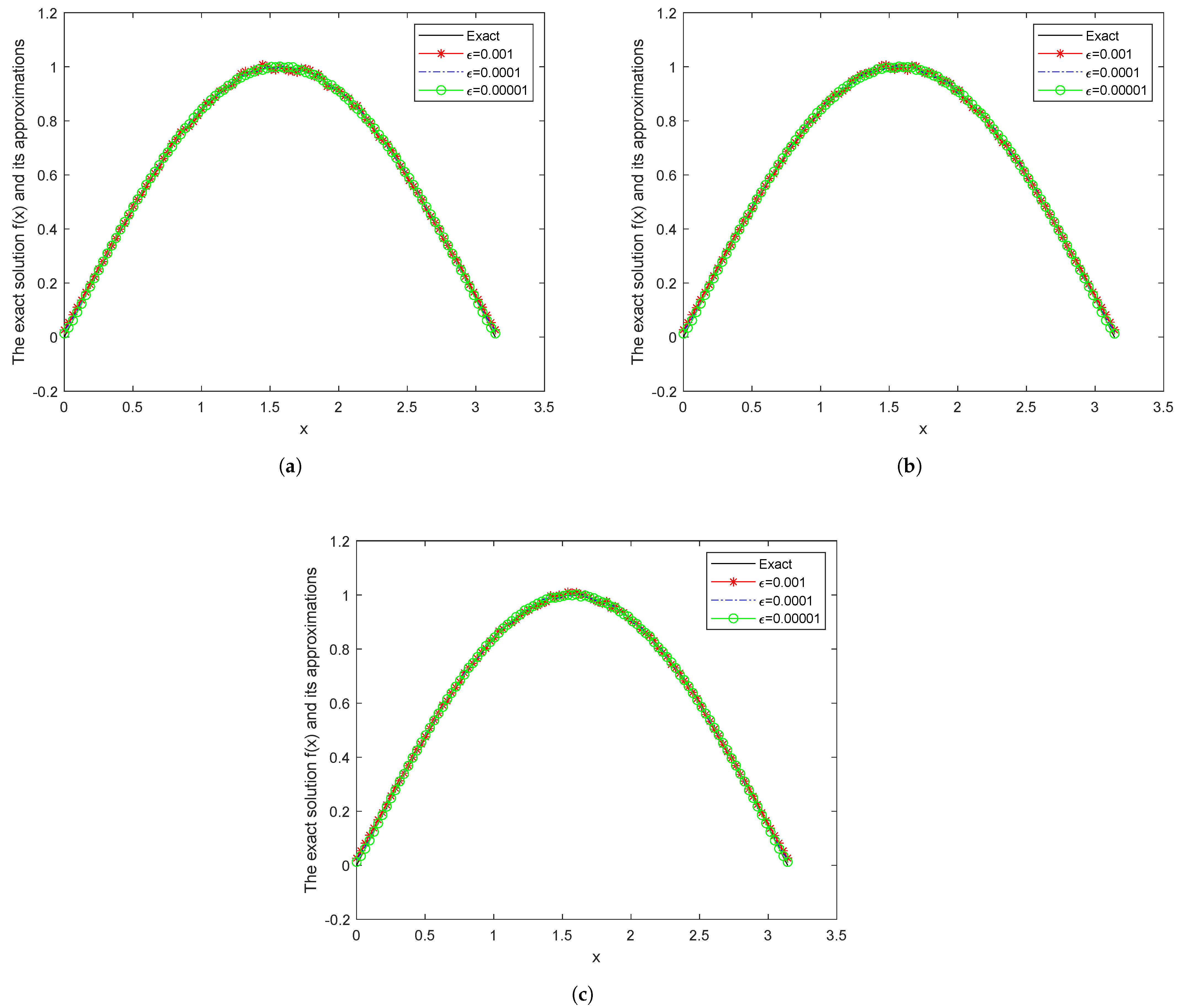
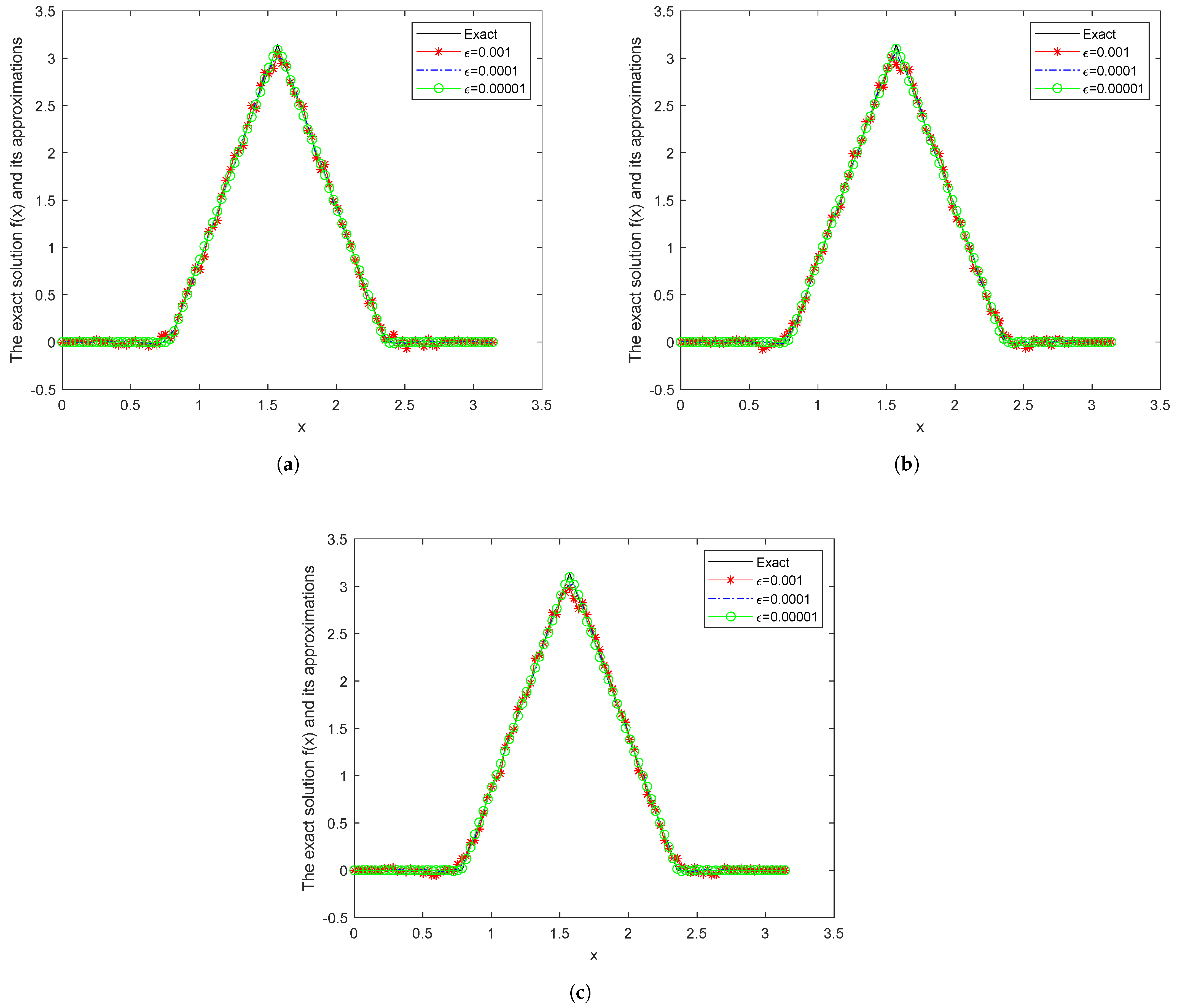
5. Numerical Results

In this section, we mainly apply Matlab software (R2024a) for simulating. Three numerical examples are given to illustrate the effectiveness and feasibility of the fractional Landweber regularization method. On the one hand, the initial functions $\varphi \left(x\right)$ and $\psi \left(x\right)$ are utilized to solve the final value function $g\left(x\right)$ in turn, that is, to solve the function $h\left(x\right)$. As we all know, this is a forward problem. On the other hand, we find the corresponding regular solution via $g\left(x\right)$ using Formula (40). Naturally, this is an inverse problem.

Let $T=1$, $\Omega =(0,\pi )$, $M=100$, $N=50$, $\tau =1.1$ in Formula (48), and some basic definitions are given as follows

$$x_i=ih(i=0,1,\cdots ,M),t_n=n\tau (n=0,1,\cdots ,N),$$

(61)

where $h={\displaystyle \frac{\pi }{M}}$ represents the step size in the spatial direction and $\tau ={\displaystyle \frac{1}{N}}$ represents the step size in the temporal direction. For the function u at each grid node, we will denote it as approximately $u_i^n\approx u(x_i,t_n)$, where $i=0,1,\dots ,M$, $n=0,1,\dots ,N$.

Consider the following one-dimensional forward problem

$$\left\{\begin{array}{cc}{D}_t^{\alpha }u(x,t)=u_{xx}(x,t)+f\left(x\right),\hfill & (x,t)\in (0,\pi )\times (0,1),1<\alpha \le 2,\hfill \\ u(0,t)=u(\pi ,t)=0,\hfill & t\in [0,1],\hfill \\ u(x,0)=\varphi \left(x\right),\hfill & x\in (0,\pi ),\hfill \\ u_t(x,0)=\psi \left(x\right),\hfill & x\in (0,\pi ),\hfill \\ u(x,1)=g\left(x\right),\hfill & x\in (0,\pi ).\hfill \end{array}\right.$$

(62)

Naturally, we use a finite difference method to discretize the terms in Formula (1) as follows:

$$D_t^{\alpha }u(x,t)\approx {\displaystyle \frac{{\tau }^{1-\alpha }}{\Gamma (3-\alpha )}}\left(b_0{\displaystyle \frac{1}{\tau }}(u_i^n-u_i^{n-1})-\sum _{j=1}^{n-1}(b_{n-j-1}-b_{n-j}){\displaystyle \frac{1}{\tau }}(u_i^j-u_i^{j-1})-b_{n-1}\psi \left(x_i\right)\right),$$

(63)

$$u_{xx}(x,t)\approx {\displaystyle \frac{u_{i+1}^n-2u_i^n+u_{i-1}^n}{h^2}},$$

(64)

where $b_0=1$, $b_k={(k+1)}^{2-\alpha }-k^{2-\alpha }$.

Let $U^n=(u_1^n,u_2^n,\cdots ,u_{M-1}^n)$, $\varphi =({\varphi }_1,{\varphi }_2,\cdots ,{\varphi }_{M-1})$, $\psi =({\psi }_1,{\psi }_2,\cdots ,{\psi }_{M-1})$, and therefore the following iterative scheme is written in terms of the discrete matrix

$$A{U}^1=f+r{\displaystyle \frac{1}{\tau }}{b}_0\varphi +r{b}_0\psi ,$$

(65)

$$A{U}^n=f+r{\displaystyle \frac{1}{\tau }}\sum _{j=2}^{n-1}(2b_{n-j}-b_{n-j-1}-b_{n-j+1})U^{j-1}+r(2b_0-b_1){\displaystyle \frac{1}{\tau }}{U}^{n-1}-r{\displaystyle \frac{1}{\tau }}(b_{n-2}-b_{n-1})\varphi \left(x\right)+r{b}_{n-1}\psi \left(x\right),$$

(66)

where A is the tridiagonal matrix, which is denoted as follows

$$A_{(M-1)\times (M-1)}=\left(\begin{array}{ccccc}r{b}_0{\displaystyle \frac{1}{\tau }}+{\displaystyle \frac{2}{h^2}}& -{\displaystyle \frac{1}{h^2}}& & & \\ -{\displaystyle \frac{1}{h^2}}& r{b}_0{\displaystyle \frac{1}{\tau }}+{\displaystyle \frac{2}{h^2}}& -{\displaystyle \frac{1}{h^2}}& & \\ & -{\displaystyle \frac{1}{h^2}}& r{b}_0{\displaystyle \frac{1}{\tau }}+{\displaystyle \frac{2}{h^2}}& -{\displaystyle \frac{1}{h^2}}& \\ & & \ddots & \ddots & \ddots \\ & & & -{\displaystyle \frac{1}{h^2}}& r{b}_0{\displaystyle \frac{1}{\tau }}+{\displaystyle \frac{2}{h^2}}\end{array}\right),$$

(67)

where $r={\displaystyle \frac{{\tau }^{1-\alpha }}{\Gamma (3-\alpha )}}$.

The final value $U^N=g$ is obtained by numerical simulation of the above difference scheme through the forward problem. In practical applications, the priori bound, E, is difficult to obtain, that is, numerical simulation is difficult under the priori regularization parameter selection rule. Subsequently, we consider this problem in a different way and undertake numerical simulation under the posteriori regularization parameter selection rule. A random disturbance is added to the final value data, $g\left(x\right)$, to generate noise data, $g^{\delta }\left(x\right)$, to participate in the calculation process of the regular solution

$$g^{\delta }=g+ϵ·randn\left(size\left(g\right)\right),$$

(68)

that is to say,

$$h^{\delta }=h+ϵ·randn\left(size\left(h\right)\right),$$

(69)

where $ϵ$ represents the relative error level and $randn(·)$ represents the normal distribution with mean 0 and variance 1. The absolute error level can be obtained according to the following equation

$$\delta =\parallel g\left(x\right)-g^{\delta }\left(x\right)\parallel =\sqrt{{\displaystyle \frac{1}{M+1}}{\sum }_{i=1}^{M+1}(g_i-g_i^{\delta })}.$$

(70)

In addition, we are also able to obtain the relative error level of $f\left(x\right)$ as follows

$$\epsilon =\sqrt{{\displaystyle \frac{\sum {(f-f^{\delta })}^2}{f^2}}}.$$

(71)

Finally, we obtain the fractional Landweber iterative regular solution using the following formula

$$f^{m,\delta }\left(x\right)=\sum _{n=1}^{\infty }{\displaystyle \frac{1-{(1-a{\left({\lambda }_n^{-1}(1-E_{\alpha ,1}(-{\lambda }_n{T}^{\alpha }))\right)}^{\beta +1})}^m}{{\lambda }_n^{-1}(1-E_{\alpha ,1}(-{\lambda }_n{T}^{\alpha }))}}{h}_n^{\delta }{X}_n\left(x\right).$$

(72)

Three numerical examples are given below, which are the smooth function, the piecewise smooth function, and the non-smooth function.

Example 1.

Smooth function

$$f\left(x\right)=sin\left(x\right),x\in [0,\pi ].$$

(73)

Example 2.

Piecewise smooth function

$$\begin{array}{c}\hfill f\left(x\right)=\left\{\begin{array}{ccc}0,\hfill & \hfill & 0\le x\le {\displaystyle \frac{\pi }{4}},\hfill \\ 4(x-{\displaystyle \frac{\pi }{4}}),\hfill & \hfill & {\displaystyle \frac{\pi }{4}}<x\le {\displaystyle \frac{\pi }{2}},\hfill \\ -4(x-{\displaystyle \frac{3\pi }{4}}),\hfill & \hfill & {\displaystyle \frac{\pi }{2}}<x\le {\displaystyle \frac{3\pi }{4}},\hfill \\ 0,\hfill & \hfill & {\displaystyle \frac{3\pi }{4}}<x\le \pi .\hfill \end{array}\right.\end{array}$$

(74)

Example 3.

Non-smooth function

$$\begin{array}{c}\hfill f\left(x\right)=\left\{\begin{array}{ccc}0,\hfill & \hfill & 0\le x\le {\displaystyle \frac{\pi }{5}},\hfill \\ 1,\hfill & \hfill & {\displaystyle \frac{\pi }{5}}<x\le {\displaystyle \frac{2\pi }{5}},\hfill \\ 0,\hfill & \hfill & {\displaystyle \frac{2\pi }{5}}<x\le {\displaystyle \frac{3\pi }{5}},\hfill \\ -1,\hfill & \hfill & {\displaystyle \frac{3\pi }{5}}<x\le {\displaystyle \frac{4\pi }{5}},\hfill \\ 0,\hfill & \hfill & {\displaystyle \frac{4\pi }{5}}<x\le \pi .\hfill \end{array}\right.\end{array}$$

(75)

Figure 1 shows a comparison between the exact solution, $f\left(x\right)$, of Example 1 and the fractional Landweber iterative regular solution, $f^{m,\delta }\left(x\right)$, for different values of $\alpha$($\alpha =1.3,1.5,1.7$) at the relative error level for $ϵ=0.001,0.0001,0.00001$.

Figure 2 shows a comparison between the exact solution, $f\left(x\right)$, of Example 2 and the fractional Landweber iterative regular solution, $f^{m,\delta }\left(x\right)$, for different values of $\alpha$($\alpha =1.3,1.5,1.7$) at the relative error level for $ϵ=0.001,0.0001,0.00001$.

Figure 3 shows a comparison between the exact solution, $f\left(x\right)$, of Example 3 and the fractional Landweber iterative regular solution, $f^{m,\delta }\left(x\right)$, for different values of $\alpha$($\alpha =1.3,1.5,1.7$) at the relative error level for $ϵ=0.001,0.0001,0.00001$.

When $\alpha =1.3,1.5,1.7$, we observe that the image fitting effectiveness under the three noise levels is exceptional, with minimal discrepancies in the effects. It is known that the fractional Landweber iterative regularization method is effective. In addition, we find that the fitting effect of $\alpha =1.3$ is better than $\alpha =1.5,1.7$. Moreover, the numerical result of Example 1 is better than those of Examples 2 and 3, because Example 1 is continuous function.

Table 1. Comparison of the iterative steps corresponding to Example 1 for various values of $ϵ$ and $\alpha$.

$\mathit{ϵ}$		0.001	0.0001	0.00001
$\alpha =1.3$	Fractional Landweber	19	92	558
$\alpha =1.5$	Fractional Landweber	20	127	616
$\alpha =1.7$	Fractional Landweber	22	130	639

,

Table 2. Comparison of the iterative steps corresponding to Example 2 for various values of $ϵ$ and $\alpha$.

$\mathit{ϵ}$		0.001	0.0001	0.00001
$\alpha =1.3$	Fractional Landweber	110	350	1314
$\alpha =1.5$	Fractional Landweber	113	391	1421
$\alpha =1.7$	Fractional Landweber	118	434	1613

, and

Table 3. Comparison of the iterative steps corresponding to Example 3 for various values of $ϵ$ and $\alpha$.

$\mathit{ϵ}$		0.001	0.0001	0.00001
$\alpha =1.3$	Fractional Landweber	749	5162	15,481
$\alpha =1.5$	Fractional Landweber	782	5637	15,724
$\alpha =1.7$	Fractional Landweber	840	5648	15,766

, respectively, show the iterative steps of Example 1, Example 2, and Example 3, corresponding to different values of $ϵ$ and $\alpha$ under the fractional Landweber iterative regularization method.

From Table 1, Table 2 and Table 3, when $\alpha$ is constant, the smaller $ϵ$ is, the longer the iterative steps of the fractional Landweber iterative regularization method are, but the better the numerical fitting effect is.

6. Conclusions

In this paper, the problem of identifying the source term for the time fractional diffusion-wave equation is investigated. The fractional Landweber iterative regularization method is adopted, and the corresponding regularization solution is obtained. After obtaining the conditional stability of the source term, $f\left(x\right)$, the error estimations are given, respectively, based on the priori regularization parameter selection rule and the posteriori regularization parameter selection rule. In addition, we give three numerical examples to verify the effectiveness and feasibility of the selected regularization method. The error estimations we obtained are order optimal based on the optimal error bound theory. In the future, we will continue our work on the inverse problem of the time fractional diffusion-wave equation, such as identifying the initial value and identifying two or three unknown terms.

References

1. Podlubny, I. Fractional Differential Equations; Elsevier: Amsterdam, The Netherlands, 1999. [Google Scholar]
2. Li, C.; Wang, Z. Mathematical analysis and the local discontinuous galerkin method for caputo–hadamard fractional partial differential equation. J. Sci. Comput. 2020, 85, 1–27. [Google Scholar] [CrossRef]
3. Gohar, M.; Li, C.; Li, Z. Finite difference methods for caputo–hadamard fractional differential equations. Mediterr. J. Math. 2020, 17, 1–26. [Google Scholar] [CrossRef]
4. Al-Salti, N.; Kerbal, E. Boundary-value problems for fractional heat equation involving Caputo-Fabrizio derivative. New Trends Math. Sci. 2016, 4, 79–89. [Google Scholar] [CrossRef]
5. Wang, J.G.; Zhou, Y.B.; Wei, T. Two regularization methods to identify a space-dependent source for the time-fractional diffusion equation-ScienceDirect. Appl. Numer. Math. 2013, 68, 39–57. [Google Scholar] [CrossRef]
6. Ruan, Z.S.; Yang, J.Z.; Lu, X.L. Tikhonov regularization method for simultaneous inversion of the source term and initial data in a time-fractional diffusion equation. E. Asian J. Appl. Math. 2015, 5, 273–300. [Google Scholar] [CrossRef]
7. Wen, J.; Liu, Z.X.; Yue, C.W.; Wang, S.J. Landweber iteration method for simultaneous inversion of the source term and initial data in a time-fractional diffusion equation. J. Appl. Math. Comput. 2022, 68, 3219–3250. [Google Scholar] [CrossRef]
8. Zeng, F.H.; Li, C.P.; Liu, F.; Turner, I. The use of finite difference/element approaches for solving the time-fractional subdiffusion equation. SIAM J. Sci. Comput. 2013, 35, A2976–A3000. [Google Scholar] [CrossRef]
9. Brunner, H.; Han, H.; Yin, D. Artificial boundary conditions and finite difference approximations for a time-fractional diffusion-wave equation on a two-dimensional unbounded spatial domain. J. Comput. Phys. 2014, 276, 541–562. [Google Scholar] [CrossRef]
10. Wei, T.; Xian, J. Determining a time-dependent coefficient in a time-fractional diffusion-wave equation with the Caputo derivative by an additional integral condition. J. Comput. Appl. Math. 2022, 404, 113910–113982. [Google Scholar] [CrossRef]
11. Yang, F.; Yan, L.L.; Liu, H.; Li, X.X. Regularization Methods for identifying the unknown source of sobolev equation with fractional Laplacian. J. Appl. Anal. Comput. 2025, 15, 198–225. [Google Scholar]
12. Garmatter, D.; Haasdonk, B.; Harrach, B. A reduced basis Landweber method for nonlinear inverse problems. Inverse Probl. 2016, 32, 035001. [Google Scholar] [CrossRef]
13. Liang, Y.Q.; Yang, F.; Li, X.X. Two Regularization Methods for Identifying the Initial Value of Time-Fractional Telegraph Equation. J. Appl. Anal. Comput. 2025. [Google Scholar] [CrossRef]
14. Cheng, W.; Fu, C.L.; Qian, Z. A modified Tikhonov regularization method for a spherically symmetric three-dimensional inverse heat conduction problem. Math. Comput. Simul. 2007, 75, 97–112. [Google Scholar] [CrossRef]
15. Liang, Y.Q.; Yang, F.; Li, X.X. A hybrid regularization method for identifying the source term and the initial value simultaneously for fractional pseudo-parabolic equation with involution. Numer. Algorithms 2024. [Google Scholar] [CrossRef]
16. Wang, J.G.; Zhou, Y.B.; Wei, T. A posteriori regularization parameter choice rule for the quasi-boundary value method for the backward time-fractional diffusion problem. Appl. Math. Lett. 2013, 26, 741–747. [Google Scholar] [CrossRef]
17. Wei, T.; Wang, J.G. A modified quasi-boundary value method for the backward time-fractional diffusion problem. Esaim-Math. Model. Num. 2014, 48, 603–621. [Google Scholar] [CrossRef]
18. Wang, Y.C.; Wu, B. On the convergence rate of an improved quasi-reversibility method for an inverse source problem of a nonlinear parabolic equation with nonlocal diffusion coefficient. Appl. Math. Lett. 2021, 5, 107491. [Google Scholar] [CrossRef]
19. Zhang, H.W.; Wei, T. A Fourier truncated regularization method for a Cauchy problem of a semi-linear elliptic equation. J. Inverse-Ill Probl. 2014, 22, 143–168. [Google Scholar] [CrossRef]
20. Yan, X.K.; He, Q.L.; Wang, Y.F. Truncated trust region method for nonlinear inverse problems and application in full-waveform inversion. J. Comput. Appl. Math. 2022, 404, 113896. [Google Scholar] [CrossRef]
21. Chen, Z.; Chan, T.H.T. A truncated generalized singular value decomposition algorithm for moving force identification with ill-posed problems. J. Sound Vib. 2017, 401, 297–310. [Google Scholar] [CrossRef]
22. Zhang, Y.X.; Fu, C.L.; Ma, Y.J. An a posteriori parameter choice rule for the truncation regularization method for solving backward parabolic problems. J. Comput. Appl. Math. 2014, 255, 150–160. [Google Scholar]
23. Murio, D.A. The mollification method and the numerical solution of the inverse heat conduction problem by finite differences. Comput. Math. Appl. 1989, 17, 1385–1396. [Google Scholar]
24. Nevolin, V.I. Using numerical solutions in the fourier method for the Fokker-Planck-Kolmogorov equation in the analysis of first-order stochastic nonlinear systems for nonlinear detectors. Radiophys. Quantum Electron. 2003, 46, 288–295. [Google Scholar]
25. Haubold, H.J.; Mathai, A.M.; Saxena, R.K. Mittag-Leffler Functions and Their Applications. J. Appl. Math. 2009, 2011, 298628. [Google Scholar] [CrossRef]
26. Pollard, H. The completely monotonic character of the Mittag-Leffler function. Bull. Amer. Math. Soc. 1948, 54, 1115–1116. [Google Scholar] [CrossRef]
27. Tautenhahn, U. Optimality for ill-posed problems under general source conditions. Numer. Funct. Anal. Optim. 2007, 19, 377–398. [Google Scholar]
28. Tautenhahn, U. Optimal stable approximations for the sideways heat equation. J. Inverse Ill-Pose Probl. 1997, 5, 287–307. [Google Scholar] [CrossRef]
29. Engl, H.W.; Hanke, M.; Neubauer, A. Regularization of Inverse Problems; Springer: Dordrecht, The Netherlands, 1996. [Google Scholar]
30. Tautenhahn, U.; Gorenflo, R. On optimal regularization methods for fractional differentiation. J. Math. Anal. Appl. 1999, 18, 449–467. [Google Scholar]
31. Tautenhahn, U.; HäMarik, U.; Hofmann, B.; Shao, Y. Conditional stability estimates for ill-posed PDE problems by using interpolation. Numer. Funct. Anal. Optim. 2013, 34, 1370–1417. [Google Scholar] [CrossRef]
Figure 1. The comparison of the exact solution,  f ( x ) , and its fractional Landweber iterative regular solution,  f m , δ ( x ) , of Example 1 with (ac α = 1.3 , 1.5 , 1.7  for  ϵ = 0.001 , 0.0001 , 0.00001 .
Symmetry 17 00554 g001
Figure 2. The comparison of the exact solution,  f ( x ) , and its fractional Landweber iterative regular solution,  f m , δ ( x ) , of Example 2 with (ac α = 1.3 , 1.5 , 1.7  for  ϵ = 0.001 , 0.0001 , 0.00001 .
Symmetry 17 00554 g002
Figure 3. The comparison of the exact solution,  f ( x ) , and its fractional Landweber iterative regular solution,  f m , δ ( x ) , of Example 3 with (ac α = 1.3 , 1.5 , 1.7  for  ϵ = 0.001 , 0.0001 , 0.00001 .
Symmetry 17 00554 g003