Parameter Estimation in Multifactor Uncertain Differential Equation with Symmetry Analysis for Stock Prediction

Abstract

Multifactor uncertain differential equations (MUDEs) are effective tools to model dynamic systems under multi-source noise. With the widespread use of MUDEs, parameter estimation as the bridge between the observed data and the MUDE becomes increasingly important. Thus, how to estimate unknown parameters in a MUDE under a multi-source noise environment is a challenge. To address this, this paper innovatively proposes a moment method to estimate the unknown parameters in a MUDE and illustrates two numerical examples to show the process of estimating parameters. Furthermore, since the system or environment is complex and constantly changing, the parameters in the MUDE are not constants but time-varying functions in many cases. Therefore, parameter estimation for time-varying functions is another challenge. In order to deal with this, this paper develops a method of parameter estimation for time-varying functions in the MUDE based on the moment method. As an application, this method of parameter estimation for time-varying functions is used to model China Merchants Bank stock.

1. Introduction

1.1. Background on SDEs and UDEs

Stochastic differential equations (SDEs) are aimed at modeling the time evolution of a dynamic system under random influence. They have been widely used in fields such as physics, medicine, biology, economics, finance, geophysics, oceanography, and others. Once the form of the SDE is determined to model a dynamic system, it typically contains unknown parameters. Since the equation itself is not completely known without the estimated parameters, it is even more impossible to obtain the result we want by using random analysis, which shows that parameter estimation in SDEs is important and fundamental. Many researchers have proposed lots of methods. In linear homogeneous SDEs, Taraskin [1] presented maximum likelihood estimation. In nonlinear homogeneous SDEs, Kutoyants [2] studied maximum likelihood estimation and Bayes estimation, Prakasa [3] proposed maximum probability estimation, Lanska [4] investigated minimum contrast estimation, Yoshida [5] introduced M-estimation, and Dietz and Kutoyants [6] studied minimum distance estimation. In nonlinear nonhomogeneous SDEs, Kutoyants [2,7] studied maximum likelihood estimation and Bayes estimation.

However, SDEs may fail to model the time evolution of a dynamic system when the white noise is described by a Wiener process because the variance of the noise tends to infinity. For example, Liu [8] pointed out two paradoxes in applying stochastic differential equations to stock prices, and Yang and Yao [9] proposed some paradoxes about applying stochastic heat equations in modeling real heat conduction. To deal with this issue, the Liu process as a likeness of the Wiener process was proposed by Liu [10]. If the white noise is described by a Liu process, then the variance of the noise is 1 rather than infinity. And for this reason, uncertain differential equations (UDEs) driven by the Liu process were established by Liu [10]. Furthermore, Ye [11] and Zhu [12] explored the theoretical basis of uncertain partial differential equations driven by the Liu process. Until now, UDEs have been applied in many fields, such as finance (Liu [8], Jia et al. [13]), optimal control (Zhu [14]), differential games (Yang and Gao [15]), and so on.

1.2. Literature Review

As UDEs find increasing applications, parameter estimation has become increasingly important. In different kinds of UDEs, parameter estimation has been studied extensively during the recent years. In first-order UDEs, Yao and Liu [16] investigated moment estimation, Liu [17] proposed generalized moment estimation, Yang et al. [18] studied minimum cover estimation, and Sheng et al. [19] investigated least squares estimation. In high-order UDEs, Liu and Yang [20] discussed moment estimation. Then, Ye and Liu [21] employed an uncertain hypothesis test [22] to test whether or not a UDE fits the observed data. As applications of UDEs, the moment method was employed to estimate the unknown parameters in an uncertain SIR model by Chen et al. [23] and those in an uncertain SEIAR model by Jia and Chen [24] to study COVID-19 spread. Moreover, Lio and Liu [25] studied how to estimate the unknown initial value of an uncertain differential equation based on observed data. Furthermore, UDEs have also applied in many fields, such as physics [26,27], chemistry [28], and finance [29,30].

These studies focused on UDEs driven by only one Liu process. This will limit the model to considering noise interference from only one source. However, in many cases, a system tends to be disturbed by multiple sources of noise. For example, in a system composed of multiple components, each component will be disturbed by noise, and then the entire system will be disturbed by multi-source noise. In this case, multifactor uncertain differential equations (MUDEs) (Li et al. [31]) are effective tools to model the system performance. As powerful tools for studying the time evolution of a dynamic system under multi-source noise, MUDEs are widely used in finance, engineering, and other fields. In order to combine observational data to conduct MUDEs, how to estimate unknown parameters in MUDEs is an important topic. To address this, Liu and Yang [32] studied parameter estimation in a pharmacokinetic model based on a MUDE. For a more general MUDE, Zhang et al. [33] tried to estimate unknown parameters by using approximate linear substitution. Wu and Liu [34] used the least squares estimation method to estimate unknown parameters in a MUDE and Liu and Zhou [35] applied a MUDE to modeling an RL Electrical Circuit.

1.3. Research Gap and Contribution

The existing literature on parameter estimation of MUDEs suggests that parameter estimation methods only apply to specific MUDEs or do not make full use of distribution information. In addition, there is a lack of discussion on the estimation of MUDEs in the case of time-varying parameters. The contribution of this paper is to introduce a new method, i.e., the moment method, to estimate unknown parameters in MUDEs. Moreover, to deal with the situation where the parameters in the MUDE are not constants but time-varying functions since the system is complex and constantly changing, this paper further study the parameter estimation for time-varying functions in the MUDE. As an application, this method of parameter estimation for time-varying functions is used to model China Merchants Bank stock.

The rest of this paper is organized as follows. Section 2 introduces an approach about how to employ the moment method to estimate unknown parameters in a MUDE. Section 3 illustrates two numerical examples to show the process of estimating unknown parameters in the MUDE. Section 4 further develops parameter estimation for time-varying functions in the MUDE, which is summarized as an algorithm in Section 5. As an application, Section 6 applies this approach of parameter estimation for time-varying functions to modeling China Merchants Bank stock. Finally, some conclusions are made in Section 7.

2. Parameter Estimation

This section tries to explore the parameter estimation in a UDE containing multiple uncertain processes, i.e., a MUDE.

Definition 1

([31]). Suppose $C_{1t},C_{2t},\cdots ,C_{nt}$ are independent Liu processes, and $f,g_1,g_2,\cdots ,g_n$ are measurable functions. Then,

$$\mathrm{d}{X}_t=f(t,X_t)\mathrm{d}t+\sum _{i=1}^n{g}_i(t,X_t)\mathrm{d}{C}_{it}$$

(1)

is called a multifactor uncertain differential equation. A solution is an uncertain process $X_t$ that satisfies (1) identically in t.

In the practical application of a MUDE, how to estimate the unknown parameters in a MUDE that fits the observed data as much as possible is a core problem. Let us consider a MUDE

$$\mathrm{d}{X}_t=f(t,X_t,\mathit{\theta })\mathrm{d}t+\sum _{i=1}^n{g}_i(t,X_t,\mathit{\theta })\mathrm{d}{C}_{it}$$

(2)

where $C_{1t},C_{2t},\cdots ,C_{nt}$ are independent Liu processes, and $f,g_1,g_2,\cdots ,g_n$ are known functions, but $\mathit{\theta }$ are unknown vectors of parameters. Suppose

$$x_{t_1},x_{t_2},\cdots ,x_{t_m}$$

are observed values of $X_t$ at the times $t_1,t_2,\cdots ,t_m$, with $t_1<t_2<\cdots <t_m$, respectively. Note that for each j, the multifactor uncertain differential Equation (2) has a different form,

$$X_{t_{j+1}}=X_{t_j}+f(t_j,X_{t_j},\mathit{\theta })(t_{j+1}-t_j)+\sum _{i=1}^n{g}_i(t_j,X_{t_j},\mathit{\theta })(C_{i{t}_{j+1}}-C_{i{t}_j}),$$

i.e.,

$$X_{t_{j+1}}-X_{t_j}-f(t_j,X_{t_j},\mathit{\theta })(t_{j+1}-t_j)=\sum _{i=1}^n{g}_i(t_j,X_{t_j},\mathit{\theta })(C_{i{t}_{j+1}}-C_{i{t}_j}).$$

Dividing both sides of the above equation by

$$\sum _{i=1}^n|g_i(t_j,X_{t_j},\mathit{\theta })|(t_{j+1}-t_j),$$

we obtain

$${\displaystyle \frac{X_{t_{j+1}}-X_{t_j}-f(t_j,X_{t_j},\mathit{\theta })(t_{j+1}-t_j)}{{\displaystyle \sum _{i=1}^n|g_i(t_j,X_{t_j},\mathit{\theta })|(t_{j+1}-t_j)}}}={\displaystyle \frac{{\displaystyle \sum _{i=1}^n{g}_i(t_j,X_{t_j},\mathit{\theta })(C_{i{t}_{j+1}}-C_{i{t}_j})}}{{\displaystyle \sum _{i=1}^n|g_i(t_j,X_{t_j},\mathit{\theta })|(t_{j+1}-t_j)}}}.$$

(3)

Substitute $X_{t_j}$ and $X_{t_{j+1}}$ with the the observed data $x_{t_j}$ and $x_{t_{j+1}}$ in the (3), and write

$$h_j\left(\mathit{\theta }\right)={\displaystyle \frac{x_{t_{j+1}}-x_{t_j}-f(t_j,x_{t_j},\mathit{\theta })(t_{j+1}-t_j)}{{\displaystyle \sum _{i=1}^n|g_i(t_j,x_{t_j},\mathit{\theta })|(t_{j+1}-t_j)}}},$$

and

$${\xi }_j={\displaystyle \frac{{\displaystyle \sum _{i=1}^n{g}_i(t_j,x_{t_j},\mathit{\theta })(C_{i{t}_{j+1}}-C_{i{t}_j})}}{{\displaystyle \sum _{i=1}^n|g_i(t_j,x_{t_j},\mathit{\theta })|(t_{j+1}-t_j)}}}.$$

On the one hand, it follows from (3) that for each j with $1\le j\le m-1$, $h_j\left(\mathit{\theta }\right)$ can be regarded as a sample of ${\xi }_j$. On the other hand, since $C_{1t},C_{2t},\cdots ,C_{nt}$ are independent Liu processes, we have

$$\begin{array}{cc}\hfill {\xi }_j& \sim {\displaystyle \frac{{\displaystyle \sum _{i=1}^n{g}_i(t_j,x_{t_j},\mathit{\theta })\mathcal{N}(0,t_{j+1}-t_j)}}{{\displaystyle \sum _{i=1}^n|g_i(t_j,x_{t_j},\mathit{\theta })|(t_{j+1}-t_j)}}}\hfill \\ & ={\displaystyle \frac{{\displaystyle \sum _{i=1}^n\mathcal{N}(0,|g_i(t_j,x_{t_j},\mathit{\theta })|(t_{j+1}-t_j))}}{{\displaystyle \sum _{i=1}^n|g_i(t_j,x_{t_j},\mathit{\theta })|(t_{j+1}-t_j)}}}\hfill \\ & ={\displaystyle \frac{{\displaystyle \mathcal{N}\left(0,\sum _{i=1}^n|g_i(t_j,x_{t_j},\mathit{\theta })|(t_{j+1}-t_j)\right)}}{{\displaystyle \sum _{i=1}^n|g_i(t_j,x_{t_j},\mathit{\theta })|(t_{j+1}-t_j)}}}\hfill \\ & =\mathcal{N}(0,1)\hfill \end{array}$$

for $j=1,2,\cdots ,m-1$. That is, ${\xi }_j,j=1,2,\cdots ,m-1$ identically follow a standard normal uncertainty distribution $\mathcal{N}(0,1)$. Thus, $h_j\left(\mathit{\theta }\right)$, $j=1,2,\cdots ,m-1$ can be regarded as $m-1$ samples of the standard normal uncertainty distribution $\mathcal{N}(0,1)$. Next, we will employ the moment method to estimate the unknown parameters. Since for each positive integer k, the k-th sample moment is

$${\displaystyle \frac{1}{m-1}}\sum _{j=1}^{m-1}{h}_j^k\left(\mathit{\theta }\right),$$

and the k-th population moment of $\mathcal{N}(0,1)$ is

$${\left({\displaystyle \frac{\sqrt{3}}{\pi }}\right)}^k{\int }_0^1{\left(ln{\displaystyle \frac{\alpha }{1-\alpha }}\right)}^k\mathrm{d}\alpha ,$$

the moment estimate $\mathit{\theta }$ should solve the system of equations

$${\displaystyle \frac{1}{m-1}}\sum _{j=1}^{m-1}{h}_j^k\left(\mathit{\theta }\right)={\left({\displaystyle \frac{\sqrt{3}}{\pi }}\right)}^k{\int }_0^1{\left(ln{\displaystyle \frac{\alpha }{1-\alpha }}\right)}^k\mathrm{d}\alpha ,k=1,2,\cdots ,p,$$

(4)

where p is the number of unknown parameters. As supplementary knowledge of population moments, the k-th population moments [36] of an uncertain variable $\xi$ with the inverse uncertainty distribution ${\Phi }^{-1}$ are

$$E\left[{\xi }^k\right]={\int }_0^1{\left({\Phi }^{-1}\left(\alpha \right)\right)}^k\mathrm{d}\alpha$$

where k is a positive integer. For example, if an uncertain variable $\xi \sim \mathcal{N}(0,1)$, then we have

$${\Phi }^{-1}\left(\alpha \right)={\displaystyle \frac{\sqrt{3}}{\pi }}ln{\displaystyle \frac{\alpha }{1-\alpha }},$$

and Ma et al. [37] provided the calculation formulas for the k-th moments of a standard normal uncertain variable, i.e.,

$$E\left[{\xi }^k\right]={\left({\displaystyle \frac{\sqrt{3}}{\pi }}\right)}^k{\int }_0^1{\left(ln{\displaystyle \frac{\alpha }{1-\alpha }}\right)}^k\mathrm{d}\alpha =(2^k-2)3^{{\displaystyle \frac{k}{2}}}|B_k|,$$

where $B_k$ are the k-th Bernoulli numbers, $k=1,2,\cdots$, respectively. Specially, we have $E\left[{\xi }^k\right]=0$ for any positive odd number k, and

$$E\left[{\xi }^2\right]=1,E\left[{\xi }^4\right]={\displaystyle \frac{21}{5}},E\left[{\xi }^6\right]={\displaystyle \frac{279}{7}}.$$

Then, let us summarize the above process with the following corollaries.

Theorem 1.

Consider a multifactor uncertain differential equation

$$\mathrm{d}{X}_t=f(t,X_t,\mathit{\theta })\mathrm{d}t+\sum _{i=1}^n{g}_i(t,X_t,\mathit{\theta })\mathrm{d}{C}_{it}$$

(5)

where $C_{1t},C_{2t},\cdots ,C_{nt}$ are independent Liu processes, and $f,g_1,g_2,\cdots ,g_n$ are known functions, but $\mathit{\theta }$ are unknown vectors of parameters. Suppose $x_{t_1},x_{t_2},\cdots ,x_{t_m}$ are observed values of $X_t$ at the times $t_1,t_2,\cdots ,t_m$, with $t_1<t_2<\cdots <t_m$, respectively. Then, the moment estimate of $\mathit{\theta }$ is the solution of the system of equations

$${\displaystyle \frac{1}{m-1}}\sum _{j=1}^{m-1}{\left({\displaystyle \frac{x_{t_{j+1}}-x_{t_j}-f(t_j,x_{t_j},\mathit{\theta })(t_{j+1}-t_j)}{{\sum }_{i=1}^n|g_i(t_j,x_{t_j},\mathit{\theta })|(t_{j+1}-t_j)}}\right)}^k={\left({\displaystyle \frac{\sqrt{3}}{\pi }}\right)}^k{\int }_0^1{\left(ln{\displaystyle \frac{\alpha }{1-\alpha }}\right)}^k\mathrm{d}\alpha$$

(6)

for $k=1,2,\cdots ,p$, where p is the number of unknown parameters.

Proof. 

It follows from (4) that the moment estimate of $\mathit{\theta }$ is the solution of the system (6). The corollary is proved. □

Corollary 1.

Consider a multifactor uncertain differential equation

$$\mathrm{d}{X}_t=\mu \mathrm{d}t+{\sigma }_1\mathrm{d}{C}_{1t}+{\sigma }_2{X}_t\mathrm{d}{C}_{2t}$$

(7)

where $C_{1t}$ and $C_{2t}$ are two independent Liu processes, and $\mu ,{\sigma }_1>0$ and ${\sigma }_2>0$ are unknown parameters. Suppose $x_{t_1},x_{t_2},\cdots ,x_{t_m}$ are observed values of $X_t$ at the times $t_1,t_2,\cdots ,t_m$, with $t_1<t_2<\cdots <t_m$, respectively. Then, the moment estimate of $\mu ,{\sigma }_1$, and ${\sigma }_2$ is the solution of the system of equations

$$\left\{\begin{array}{c}{\displaystyle \frac{1}{m-1}}\sum _{j=1}^{m-1}{\displaystyle \frac{x_{t_{j+1}}-x_{t_j}-\mu (t_{j+1}-t_j)}{(|{\sigma }_1|+|{\sigma }_2{x}_{t_j}|)(t_{j+1}-t_j)}}=0\hfill \\ {\displaystyle \frac{1}{m-1}}\sum _{j=1}^{m-1}{\left({\displaystyle \frac{x_{t_{j+1}}-x_{t_j}-\mu (t_{j+1}-t_j)}{(|{\sigma }_1|+|{\sigma }_2{x}_{t_j}|)(t_{j+1}-t_j)}}\right)}^2=1\hfill \\ {\displaystyle \frac{1}{m-1}}\sum _{j=1}^{m-1}{\left({\displaystyle \frac{x_{t_{j+1}}-x_{t_j}-\mu (t_{j+1}-t_j)}{(|{\sigma }_1|+|{\sigma }_2{x}_{t_j}|)(t_{j+1}-t_j)}}\right)}^3=0.\hfill \end{array}\right.$$

(8)

Proof. 

Since there are only three unknown parameters in (7) and the first three moments of $\mathcal{N}(0,1)$ are $0,1,0$, the system of Equation (6) becomes (8). It follows from Theorem 1 that the moment estimate of $\mu ,{\sigma }_1$, and ${\sigma }_2$ is the solution of the system of Equation (8). The corollary is proved. □

Corollary 2.

Consider a multifactor uncertain differential equation

$$\mathrm{d}{X}_t=cos({\mu }_{1}t+{\mu }_2{X}_t)\mathrm{d}t+sin\left({\sigma }_1{X}_t\right)\mathrm{d}{C}_{1t}+cos\left({\sigma }_2{X}_t\right)\mathrm{d}{C}_{2t}$$

(9)

where $C_{1t}$ and $C_{2t}$ are two independent Liu processes, and ${\mu }_1,{\mu }_2,{\sigma }_1>0$ and ${\sigma }_2>0$ are unknown parameters. Suppose $x_{t_1},x_{t_2},\cdots ,x_{t_m}$ are observed values of $X_t$ at the times $t_1,t_2,\cdots ,t_m$, with $t_1<t_2<\cdots <t_m$, respectively. Then, the moment estimate of ${\mu }_1,{\mu }_2,{\sigma }_1$, and ${\sigma }_2$ is the solution of the system of equations

$$\left\{\begin{array}{c}{\displaystyle \frac{1}{m-1}}\sum _{j=1}^{m-1}{\displaystyle \frac{x_{t_{j+1}}-x_{t_j}-cos({\mu }_1{t}_j+{\mu }_2{x}_{t_j})(t_{j+1}-t_j)}{(|sin\left({\sigma }_1{x}_{t_j}\right)|+|cos\left({\sigma }_2{x}_{t_j}\right)|)(t_{j+1}-t_j)}}=0\hfill \\ {\displaystyle \frac{1}{m-1}}\sum _{j=1}^{m-1}{\left({\displaystyle \frac{x_{t_{j+1}}-x_{t_j}-cos({\mu }_1{t}_j+{\mu }_2{x}_{t_j})(t_{j+1}-t_j)}{(|sin\left({\sigma }_1{x}_{t_j}\right)|+|cos\left({\sigma }_2{x}_{t_j}\right)|)(t_{j+1}-t_j)}}\right)}^2=1\hfill \\ {\displaystyle \frac{1}{m-1}}\sum _{j=1}^{m-1}{\left({\displaystyle \frac{x_{t_{j+1}}-x_{t_j}-cos({\mu }_1{t}_j+{\mu }_2{x}_{t_j})(t_{j+1}-t_j)}{(|sin\left({\sigma }_1{x}_{t_j}\right)|+|cos\left({\sigma }_2{x}_{t_j}\right)|)(t_{j+1}-t_j)}}\right)}^3=0\hfill \\ {\displaystyle \frac{1}{m-1}}\sum _{j=1}^{m-1}{\left({\displaystyle \frac{x_{t_{j+1}}-x_{t_j}-cos({\mu }_1{t}_j+{\mu }_2{x}_{t_j})(t_{j+1}-t_j)}{(|sin\left({\sigma }_1{x}_{t_j}\right)|+|cos\left({\sigma }_2{x}_{t_j}\right)|)(t_{j+1}-t_j)}}\right)}^4={\displaystyle \frac{21}{5}}.\hfill \end{array}\right.$$

(10)

Proof. 

Since there are only four unknown parameters in (9) and the first four moments of $\mathcal{N}(0,1)$ are $0,1,0,21/5$, the system of Equation (6) becomes (10). It follows from Theorem 1 that the moment estimate of ${\mu }_1,{\mu }_2,{\sigma }_1$, and ${\sigma }_2$ is the solution of the system of Equation (10). The corollary is proved. □

Corollary 3.

Consider a multifactor uncertain differential equation

$$\mathrm{d}{X}_t=(a-b{X}_t)\mathrm{d}t+\mu \mathrm{d}{C}_{1t}+\sigma X_t\mathrm{d}{C}_{2t}$$

(11)

where $C_{1t}$ and $C_{2t}$ are two independent Liu processes, and $a,b,\mu >0$ and $\sigma >0$ are unknown parameters. Suppose $x_{t_1},x_{t_2},\cdots ,x_{t_m}$ are observed values of $X_t$ at the times $t_1,t_2,\cdots ,t_m$, with $t_1<t_2<\cdots <t_m$, respectively. Then, the moment estimate of $a,b,\mu$ and σ is the solution of the system of equations

$$\left\{\begin{array}{c}{\displaystyle \frac{1}{m-1}}\sum _{j=1}^{m-1}{\displaystyle \frac{x_{t_{j+1}}-x_{t_j}-(a-b{x}_{t_j})(t_{j+1}-t_j)}{(|\mu |+|\sigma x_{t_j}|)(t_{j+1}-t_j)}}=0\hfill \\ {\displaystyle \frac{1}{m-1}}\sum _{j=1}^{m-1}{\left({\displaystyle \frac{x_{t_{j+1}}-x_{t_j}-(a-b{x}_{t_j})(t_{j+1}-t_j)}{(|\mu |+|\sigma x_{t_j}|)(t_{j+1}-t_j)}}\right)}^2=1\hfill \\ {\displaystyle \frac{1}{m-1}}\sum _{j=1}^{m-1}{\left({\displaystyle \frac{x_{t_{j+1}}-x_{t_j}-(a-b{x}_{t_j})(t_{j+1}-t_j)}{(|\mu |+|\sigma x_{t_j}|)(t_{j+1}-t_j)}}\right)}^3=0\hfill \\ {\displaystyle \frac{1}{m-1}}\sum _{j=1}^{m-1}{\left({\displaystyle \frac{x_{t_{j+1}}-x_{t_j}-(a-b{x}_{t_j})(t_{j+1}-t_j)}{(|\mu |+|\sigma x_{t_j}|)(t_{j+1}-t_j)}}\right)}^4={\displaystyle \frac{21}{5}}.\hfill \end{array}\right.$$

(12)

Proof. 

Since there are only four unknown parameters in (11) and the first four moments of $\mathcal{N}(0,1)$ are $0,1,0,21/5$, the system of Equation (6) becomes (12). It follows from Theorem 1 that the moment estimate of ${\mu }_1,{\mu }_2,{\sigma }_1$ and ${\sigma }_2$ is the solution of the system of Equation (12). The corollary is proved. □

3. Numerical Examples

Example 1.

Let us apply the method in Section 2 to estimating the unknown parameters $\mu ,{\sigma }_1>0$ and ${\sigma }_2>0$ in the multifactor uncertain differential equation

$$\mathrm{d}{X}_t=\mu \mathrm{d}t+{\sigma }_1\mathrm{d}{C}_{1t}+{\sigma }_2{X}_t\mathrm{d}{C}_{2t}$$

(13)

based on the observed data shown in

Table 1. Observed data in Example 1.

t	0.24	0.49	0.84	1.1	1.33	1.58	1.8	2.05	2.44
$x_t$	3.74	4.85	3.95	4.31	1.67	1.17	1.98	2.36	2.03
t	2.7	3.08	3.34	3.62	3.98	4.35	4.57	4.81	5.15
$x_t$	3.13	5.16	2.73	3.14	5.72	6.48	10.23	10	11.88
t	5.43	5.68	5.95	6.28	6.61	6.94	7.23
$x_t$	14.51	13.39	10.09	5.94	7.96	8.53	10.92

and Figure 1, which are generated by the simulation of the following equation:

$$\mathrm{d}{X}_t=1.5\mathrm{d}t+1.5\mathrm{d}{C}_{1t}+2X_t\mathrm{d}{C}_{2t}.$$

It follows from Corollary 1 that the moment estimate of $\mu ,{\sigma }_1$ and ${\sigma }_2$ is the solution of the system of equations

$$\left\{\begin{array}{c}{\displaystyle \frac{1}{24}}\sum _{j=1}^{24}{\displaystyle \frac{x_{t_{j+1}}-x_{t_j}-\mu (t_{j+1}-t_j)}{(|{\sigma }_1|+|{\sigma }_2{x}_{t_j}|)(t_{j+1}-t_j)}}=0\hfill \\ {\displaystyle \frac{1}{24}}\sum _{j=1}^{24}{\left({\displaystyle \frac{x_{t_{j+1}}-x_{t_j}-\mu (t_{j+1}-t_j)}{(|{\sigma }_1|+|{\sigma }_2{x}_{t_j}|)(t_{j+1}-t_j)}}\right)}^2=1\hfill \\ {\displaystyle \frac{1}{24}}\sum _{j=1}^{24}{\left({\displaystyle \frac{x_{t_{j+1}}-x_{t_j}-\mu (t_{j+1}-t_j)}{(|{\sigma }_1|+|{\sigma }_2{x}_{t_j}|)(t_{j+1}-t_j)}}\right)}^3=0.\hfill \end{array}\right.$$

By using Matlab (Matlab R2020a, optimization toolbox), we can calculate that the root of the above system of equations is

$$\mu =1.7472,{\sigma }_1=1.4513,{\sigma }_2=1.9155.$$

Thus, the multifactor uncertain differential equation should be

$$\mathrm{d}{X}_t=1.7472\mathrm{d}t+1.4513\mathrm{d}{C}_{1t}+1.9155X_t\mathrm{d}{C}_{2t}.$$

The mean relative error between the estimated value and the real value of the parameters is

$$\mathrm{MRE}={\displaystyle \frac{{\displaystyle \left|\frac{1.7472-1.5}{1.5}\right|+\left|\frac{1.4513-1.5}{1.5}\right|+\left|\frac{1.9155-2}{2}\right|}}{3}}=0.0798.$$

This indicates that the estimated value is close to the real value, and thus the estimate is appropriate.

Example 2.

Let us apply the method in Section 2 to estimating the unknown parameters ${\mu }_1,{\mu }_2,{\sigma }_1>0$, and ${\sigma }_2>0$ in the multifactor uncertain differential equation

$$\mathrm{d}{X}_t=cos({\mu }_{1}t+{\mu }_2{X}_t)\mathrm{d}t+sin\left({\sigma }_1{X}_t\right)\mathrm{d}{C}_{1t}+cos\left({\sigma }_2{X}_t\right)\mathrm{d}{C}_{2t}$$

(14)

based on the observed data shown in

Table 2. Observed data in Example 2.

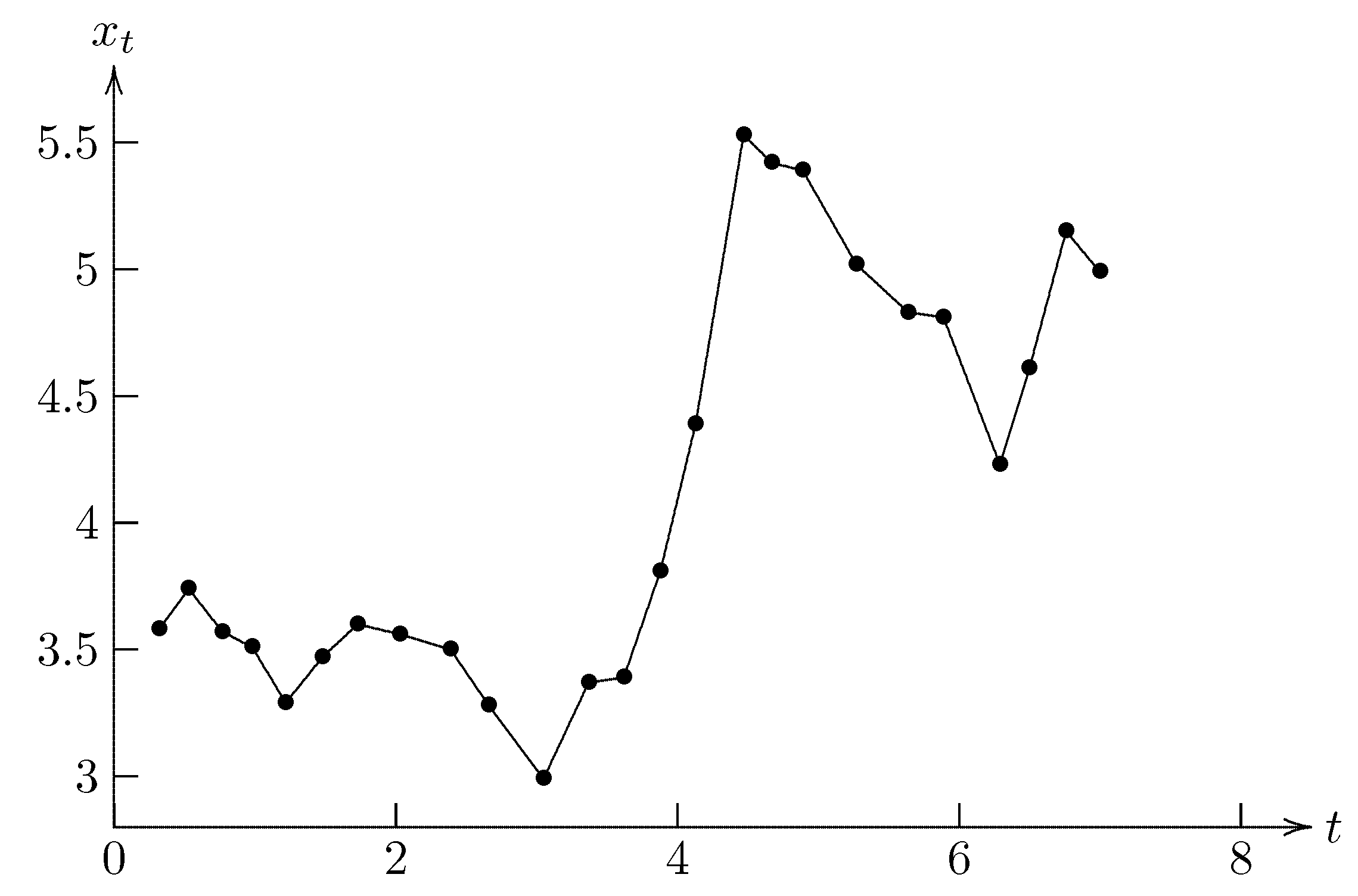
t	0.32	0.53	0.77	0.98	1.22	1.48	1.73	2.03	2.39
$x_t$	3.58	3.74	3.57	3.51	3.29	3.47	3.6	3.56	3.5
t	2.66	3.05	3.37	3.62	3.88	4.13	4.47	4.67	4.89
$x_t$	3.28	2.99	3.37	3.39	3.81	4.39	5.53	5.42	5.39
t	5.27	5.64	5.89	6.29	6.5	6.76	7
$x_t$	5.02	4.83	4.81	4.23	4.61	5.15	4.99

and Figure 2, which are generated by the simulation of the following equation:

$$\mathrm{d}{X}_t=cos(t+X_t)\mathrm{d}t+sin\left(X_t\right)\mathrm{d}{C}_{1t}+cos\left(X_t\right)\mathrm{d}{C}_{2t}.$$

It follows from Corollary 2 that the moment estimate of ${\mu }_1,{\mu }_2,{\sigma }_1$ and ${\sigma }_2$ is the solution of the system of equations

$$\left\{\begin{array}{c}{\displaystyle \frac{1}{24}}\sum _{j=1}^{24}{\displaystyle \frac{x_{t_{j+1}}-x_{t_j}-cos({\mu }_1{t}_j+{\mu }_2{x}_{t_j})(t_{j+1}-t_j)}{(|sin\left({\sigma }_1{x}_{t_j}\right)|+|cos\left({\sigma }_2{x}_{t_j}\right)|)(t_{j+1}-t_j)}}=0\hfill \\ {\displaystyle \frac{1}{24}}\sum _{j=1}^{24}{\left({\displaystyle \frac{x_{t_{j+1}}-x_{t_j}-cos({\mu }_1{t}_j+{\mu }_2{x}_{t_j})(t_{j+1}-t_j)}{(|sin\left({\sigma }_1{x}_{t_j}\right)|+|cos\left({\sigma }_2{x}_{t_j}\right)|)(t_{j+1}-t_j)}}\right)}^2=1\hfill \\ {\displaystyle \frac{1}{24}}\sum _{j=1}^{24}{\left({\displaystyle \frac{x_{t_{j+1}}-x_{t_j}-cos({\mu }_1{t}_j+{\mu }_2{x}_{t_j})(t_{j+1}-t_j)}{(|sin\left({\sigma }_1{x}_{t_j}\right)|+|cos\left({\sigma }_2{x}_{t_j}\right)|)(t_{j+1}-t_j)}}\right)}^3=0\hfill \\ {\displaystyle \frac{1}{24}}\sum _{j=1}^{24}{\left({\displaystyle \frac{x_{t_{j+1}}-x_{t_j}-cos({\mu }_1{t}_j+{\mu }_2{x}_{t_j})(t_{j+1}-t_j)}{(|sin\left({\sigma }_1{x}_{t_j}\right)|+|cos\left({\sigma }_2{x}_{t_j}\right)|)(t_{j+1}-t_j)}}\right)}^4={\displaystyle \frac{21}{5}}.\hfill \end{array}\right.$$

By using Matlab (Matlab R2020a, optimization toolbox), we can calculate that the root of the above system of equations is

$${\mu }_1=1.0802,{\mu }_2=0.9798,{\sigma }_1=1.0910,{\sigma }_2=0.9199.$$

Thus, the multifactor uncertain differential equation should be

$$\mathrm{d}{X}_t=cos(1.0802t+0.9798X_t)\mathrm{d}t+sin\left(1.0910X_t\right)\mathrm{d}{C}_{1t}+cos\left(0.9199X_t\right)\mathrm{d}{C}_{2t}.$$

The mean relative error between the estimated value and the real value of the parameters is

$$\mathrm{MRE}={\displaystyle \frac{{\displaystyle \left|\frac{1.0802-1}{1}\right|+\left|\frac{0.9798-1}{1}\right|+\left|\frac{1.0910-1}{1}\right|+\left|\frac{0.9199-1}{1}\right|}}{4}}=0.0679.$$

This indicates that the estimated value is close to the real value, and thus the estimate is appropriate.

4. Parameter Estimation for Time-Varying Functions

The theory of mean reversion emphasizes that stock price shows a certain property of mean reversion in the long run, although it is affected by many factors. In the financial field, mean reversion theory is widely used and has proven to be effective. Poterba and Summers [38] supported this view by analyzing the US stock market. On the other hand, the noise of stock price growth is partly due to price factors related to the stock’s own price, and partly due to price factors unrelated to the stock’s own price. In order to describe these two sources of different noise, the stock price $X_t$ is usually modeled by the multifactor mean-reverting model (11) in uncertain finance, i.e.,

$$\mathrm{d}{X}_t=(a-b{X}_t)\mathrm{d}t+\mu \mathrm{d}{C}_{1t}+\sigma X_t\mathrm{d}{C}_{2t}.$$

However, since the situation in the real stock market is complex and rapidly changing, the parameters $a,b,\mu ,\sigma$ are not constants but time-varying functions. Although the general trend makes stock price subject to the multifactor mean-reverting model, the parameters of the multifactor mean-reverting model may change over time. Thus, it is more appropriate to assume that the stock price $X_t$ follows the general multifactor mean-reverting model,

$$\mathrm{d}{X}_t=(a_t-b_t{X}_t)\mathrm{d}t+{\mu }_t\mathrm{d}{C}_{1t}+{\sigma }_t{X}_t\mathrm{d}{C}_{2t}.$$

(15)

Suppose $x_{t_1},x_{t_2},\cdots ,x_{t_m}$ are observed data of stock price $X_t$ at the times $t_1,t_2,\cdots ,t_m$, with $t_1<t_2<\cdots <t_m$, respectively. The main idea of estimating $a_t,b_t,{\mu }_t,{\sigma }_t$ based on the observed data $x_{t_1},x_{t_2},\cdots ,x_{t_m}$ is to suppose that $a_t,b_t,{\mu }_t,{\sigma }_t$ remain constant over a small time interval, and thus, in each time interval, they can be estimated with the moment method discussed in Section 2. The detailed process is as follows.

First, let us estimate $a_{t_1},b_{t_1},{\mu }_{t_1},{\sigma }_{t_1}$ with the data $x_{t_1},x_{t_2},\cdots ,x_{t_k}$, where k is a given step. Suppose the model (15) has a different form,

$$X_{t_{j+1}}=X_{t_j}+(a_{t_1}-b_{t_1}{X}_{t_j})+{\mu }_{t_1}(C_{1t_{j+1}}-C_{1t_j})+{\sigma }_{t_1}{X}_{t_j}(C_{2t_{j+1}}-C_{2t_j}),j=1,2,\cdots ,k-1.$$

It follows from Corollary 3 that the moment estimate of $a_{t_1},b_{t_1},{\mu }_{t_1},{\sigma }_{t_1}$ solves the system of equations

$$\left\{\begin{array}{c}{\displaystyle \frac{1}{k-1}}\sum _{j=1}^{k-1}{\displaystyle \frac{x_{t_{j+1}}-x_{t_j}-(a_{t_1}-b_{t_1}{x}_{t_j})(t_{j+1}-t_j)}{(|{\mu }_{t_1}|+|{\sigma }_{t_1}{x}_{t_j}|)(t_{j+1}-t_j)}}=0\hfill \\ {\displaystyle \frac{1}{k-1}}\sum _{j=1}^{k-1}{\left({\displaystyle \frac{x_{t_{j+1}}-x_{t_j}-(a_{t_1}-b_{t_1}{x}_{t_j})(t_{j+1}-t_j)}{(|{\mu }_{t_1}|+|{\sigma }_{t_1}{x}_{t_j}|)(t_{j+1}-t_j)}}\right)}^2=1\hfill \\ {\displaystyle \frac{1}{k-1}}\sum _{j=1}^{k-1}{\left({\displaystyle \frac{x_{t_{j+1}}-x_{t_j}-(a_{t_1}-b_{t_1}{x}_{t_j})(t_{j+1}-t_j)}{(|{\mu }_{t_1}|+|{\sigma }_{t_1}{x}_{t_j}|)(t_{j+1}-t_j)}}\right)}^3=0\hfill \\ {\displaystyle \frac{1}{k-1}}\sum _{j=1}^{k-1}{\left({\displaystyle \frac{x_{t_{j+1}}-x_{t_j}-(a_{t_1}-b_{t_1}{x}_{t_j})(t_{j+1}-t_j)}{(|{\mu }_{t_1}|+|{\sigma }_{t_1}{x}_{t_j}|)(t_{j+1}-t_j)}}\right)}^4={\displaystyle \frac{21}{5}}.\hfill \end{array}\right.$$

Next, let us estimate $a_{t_2},b_{t_2},{\mu }_{t_2},{\sigma }_{t_2}$ with the data $x_{t_2},x_{t_3},\cdots ,x_{t_{k+1}}$. It follows from Corollary 3 that the moment estimate of $a_{t_2},b_{t_2},{\mu }_{t_2},{\sigma }_{t_2}$ solves the system of equations

$$\left\{\begin{array}{c}{\displaystyle \frac{1}{k-1}}\sum _{j=2}^k{\displaystyle \frac{x_{t_{j+1}}-x_{t_j}-(a_{t_2}-b_{t_2}{x}_{t_j})(t_{j+1}-t_j)}{(|{\mu }_{t_2}|+|{\sigma }_{t_2}{x}_{t_j}|)(t_{j+1}-t_j)}}=0\hfill \\ {\displaystyle \frac{1}{k-1}}\sum _{j=2}^k{\left({\displaystyle \frac{x_{t_{j+1}}-x_{t_j}-(a_{t_2}-b_{t_2}{x}_{t_j})(t_{j+1}-t_j)}{(|{\mu }_{t_2}|+|{\sigma }_{t_2}{x}_{t_j}|)(t_{j+1}-t_j)}}\right)}^2=1\hfill \\ {\displaystyle \frac{1}{k-1}}\sum _{j=2}^k{\left({\displaystyle \frac{x_{t_{j+1}}-x_{t_j}-(a_{t_2}-b_{t_2}{x}_{t_j})(t_{j+1}-t_j)}{(|{\mu }_{t_2}|+|{\sigma }_{t_2}{x}_{t_j}|)(t_{j+1}-t_j)}}\right)}^3=0\hfill \\ {\displaystyle \frac{1}{k-1}}\sum _{j=2}^k{\left({\displaystyle \frac{x_{t_{j+1}}-x_{t_j}-(a_{t_2}-b_{t_2}{x}_{t_j})(t_{j+1}-t_j)}{(|{\mu }_{t_2}|+|{\sigma }_{t_2}{x}_{t_j}|)(t_{j+1}-t_j)}}\right)}^4={\displaystyle \frac{21}{5}}.\hfill \end{array}\right.$$

As an analogy, we can obtain the estimated values $a_{t_i},b_{t_i},{\mu }_{t_i},{\sigma }_{t_i}$, where $i=1,2,\cdots ,m-k+1$.

5. Algorithm for General Multifactor Mean-Reverting Model

The following algorithm is designed to summarize the method of parameter estimation for time-varying functions discussed in the previous section.

Step 1: With the data $x_{t_1},x_{t_2},\cdots ,x_{t_m}$ and a given step k, for each i ($i=1,2,\cdots ,m-k+1$), calculate the moment estimate of $a_{t_i},b_{t_i},{\mu }_{t_i},{\sigma }_{t_i}$ by solving the system of Equation (12) based on the data $x_{t_i},x_{t_{i+1}},\cdots ,x_{t_{i+k-2}}$.

Step 2: For each i ($i=1,2,\cdots ,m-k+1$), calculate the forecast value ${\widehat{x}}_{t_i}$ by

$${\widehat{x}}_{t_i}={\int }_0^1{X}_{t_i}^{\alpha }\mathrm{d}\alpha ,$$

and the confidence interval $[X_{t_i}^{\beta },X_{t_i}^{1-\beta }]$ at a given confidence level $\beta$, where $X_{t_i}^{\alpha }$ is the $\alpha$-path of (15) with the initial point $x_{t_i}$.

In order to select the step k of the above algorithm, we focus on the prediction error (PE) of the last actual data $x_{t_m}$, and want to minimize that prediction error. Thus, we define

$$\mathrm{PE}\left(k\right)=|x_{t_m}-{\widehat{x}}_{t_m}|$$

where ${\widehat{x}}_{t_m}$ is the forecast value of $x_{t_m}$ based on the k data in front of $x_{t_m}$, i.e., $x_{t_{m-k+1}},x_{t_{m-k+2}}$, $\cdots ,x_{t_{m-1}}$. Then, the solution of the following minimization problem

$$\underset{k}{min}\mathrm{PE}\left(k\right)$$

is the step to choose.

6. Application to China Merchants Bank Stock

The data included in this study are the closing price of China Merchants Bank for 300 trading days from 3 April 2019 to 29 June 2020. The unit is CNY 0.1 (see Figure 3a). Suppose that the closing price of China Merchants Bank follows a general multifactor mean-reverting model (15). Then, we employ the algorithm in Section 5 to simulate to obtain parameter estimations and predictions.

At first, we calculate the PE(k) for each step k with $1\le k\le 15$, which is shown in Figure 3b. When $k=4$, PE(k) reaches the minimum 2.64. Thus, we take the step $k=4$. By following the algorithm in Section 5 and taking a confidence level of $\beta =80\%$, we obtain the forecast price and forecast high and low prices of China Merchants Bank shown in Figure 4, the parameter estimations of $a_t$ and $b_t$ shown in Figure 5, and the parameter estimations of ${\mu }_t$ and ${\sigma }_t$ shown in Figure 6. From Figure 4, we can see the forecast high and low prices are basically symmetrical with respect to the real price. From Figure 5 and Figure 6, the parameters in multifactor mean-reverting model (15) change greatly, which indicates that they are not constants but time-varying functions.

The forecast value of the closing price of China Merchants Bank on the next trading day (i.e., 30 June 2020) is 337.67, and the $80\%$-confidence interval is

$$[320.96,354.12].$$

The actual closing price on 30 June 2020 was 337.2, with the low and high prices on that day being 336.4 and 339.6, respectively. From the view of forecast results, our method is efficient. In addition, on the one hand, for each $i=5,6,\cdots ,300$, if the real stock price $x_{t_i}$ falls in the corresponding $80\%$ confidence interval $[X_{t_i}^{0.2},X_{t_i}^{0.8}]$, then the prediction at time $t_i$ is considered to be successful. Then, that is 278 successes in total. The correct rate of forecasting is

$$r={\displaystyle \frac{278}{296}}=93.6\%.$$

On the other hand, for each $i=5,6,\cdots ,300$, compute the mean relative error between the predicted stock prices and the real stock prices,

$$\mathrm{MRE}={\displaystyle \frac{1}{296}}\sum _{i=5}^{300}\left|{\displaystyle \frac{{\widehat{x}}_{t_i}-x_{t_i}}{x_{t_i}}}\right|=0.49\%,$$

where ${\widehat{x}}_{t_i}$ and $x_{t_i}$ are the predicted stock price and the real stock price, respectively. This index means that the difference between the predicted stock price and the real stock price is $0.49\%$ on average, which indicates that our method and the prediction effect are generally efficient.

7. Conclusions

MUDEs are effective tools to model dynamic systems under multi-source noise. With the widespread use of MUDEs, how to estimate unknown parameters in a MUDE has become an important research topic. To address this, this paper innovatively introduced an approach to employ the moment method to estimate parameters in a MUDE under the framework of uncertainty theory. Then, two numerical examples were illustrated to show the estimation process.

Furthermore, traditional parameter estimation methods are limited to the fact that the parameters in the MUDE are fixed constants. However, since the system or environment is complex and constantly changing, the parameters in the MUDE are not constants but time-varying functions in many cases. In order to deal with the situation where the parameters in the MUDE are not constants but time-varying functions, this paper further studied the parameter estimation for time-varying functions in a MUDE. As an application, this method was used to model China Merchants Bank stock.

In the future, the research frontiers MUDEs can be approached in two directions. One is the research innovation of estimation methods. Researchers can further apply the generalized moment method in parameter estimation of MUDEs to make up for the defect that the equations of moment estimation may have no solution. In addition, more methods of MUDEs can be studied, such as initial value estimation, maximum likelihood estimation, consistency of estimators, and non-gaussian moments. The other is the expansion of application field. Since MUDEs are tools to deal with multi-source noise, they can be used for system modeling in multi-complex scenes and multi-noise environments. Thus, the application fields of MUDEs can be expanded, such as economics, system modeling, and reliability analysis.

References

- Taraskin, A. On the asymptotic normality of vector-valued stochastic integrals and estimates of drift parameters of a multidimensional diffusion process. Theory Probab. Math. Stat. 1974, 2, 209–224. [Google Scholar]
- Kutoyants, Y.A. Estimation of the trend parameter of a diffusion process in the smooth case. Theory Probab. Its Appl. 1977, 22, 399–406. [Google Scholar] [CrossRef]
- Prakasa, R. The Bernstein-von Mises theorem for a class of diffusion processes. Theory Random Process. 1980, 9, 95–101. [Google Scholar]
- Lanksa, V. Minimum contrast estimation in diffusion processes. J. Appl. Probab. 1979, 16, 65–75. [Google Scholar] [CrossRef]
- Yoshida, N. Robust M-estimators in diffusion processes. Ann. Inst. Stat. Math. 1988, 40, 799–820. [Google Scholar] [CrossRef]
- Dietz, H.M.; Kutoyants, Y.A. A class of minimum-distance estimators for diffusion processes with ergodic properties. Stat. Risk Model. 1997, 15, 211–227. [Google Scholar] [CrossRef]
- Kutoyants, Y.A. Parameter estimation for stochastic processes. Acta Math. 1984, 112, 1–40. [Google Scholar]
- Liu, B. Toward uncertain finance theory. J. Uncertain. Anal. Appl. 2013, 1, 1. [Google Scholar] [CrossRef]
- Yang, X.; Yao, K. Uncertain partial differential equation with application to heat conduction. Fuzzy Optim. Decis. Mak. 2017, 16, 379–403. [Google Scholar] [CrossRef]
- Liu, B. Some research problems in uncertainty theory. J. Uncertain Syst. 2009, 3, 3–10. [Google Scholar]
- Ye, T.Q. Partial derivatives of uncertain fields and uncertain partial differential equations. Fuzzy Optim. Decis. Mak. 2024, 23, 199–217. [Google Scholar] [CrossRef]
- Zhu, Y. On uncertain partial differential equations. Fuzzy Optim. Decis. Mak. 2024, 23, 219–237. [Google Scholar] [CrossRef]
- Jia, L.; Li, D.; Guo, F.; Zhang, B. Knock-in options of mean-reverting stock model with floating interest rate in uncertain environment. Int. J. Gen. Syst. 2024, 53, 331–351. [Google Scholar] [CrossRef]
- Zhu, Y. Uncertain optimal control with application to a portfolio selection model. Cybern. Syst. 2010, 41, 535–547. [Google Scholar] [CrossRef]
- Yang, X.; Gao, J. Uncertain differential games with application to capitalism. J. Uncertain. Anal. Appl. 2013, 1, 17. [Google Scholar] [CrossRef]
- Yao, K.; Liu, B. Parameter estimation in uncertain differential equations. Fuzzy Optim. Decis. Mak. 2020, 19, 1–12. [Google Scholar] [CrossRef]
- Liu, Z. Generalized moment estimation for uncertain differential equations. Appl. Math. Comput. 2021, 392, 125724. [Google Scholar] [CrossRef]
- Yang, X.F.; Liu, Y.; Park, G. Parameter estimation of uncertain differential equation with application to financial market. Chaos Solitons Fract. 2021, 139, 110026. [Google Scholar] [CrossRef]
- Sheng, Y.H.; Yao, K.; Chen, X. Least squares estimation in uncertain differential equations. IEEE Trans. Fuzzy Syst. 2020, 28, 2651–2655. [Google Scholar] [CrossRef]
- Liu, Z.; Yang, Y. Moment estimations for parameters in high-order uncertain differential equations. J. Intell. Fuzzy Syst. 2020, 39, 1–9. [Google Scholar] [CrossRef]
- Ye, T.Q.; Liu, B. Uncertain hypothesis test for uncertain differential equations. Fuzzy Optim. Decis. Mak. 2023, 22, 195–211. [Google Scholar] [CrossRef]
- Ye, T.Q.; Liu, B. Uncertain hypothesis test with application to uncertain regression analysis. Fuzzy Optim. Decis. Mak. 2022, 21, 157–174. [Google Scholar] [CrossRef]
- Chen, X.; Li, J.; Xiao, C.; Yang, P. Numerical solution and parameter estimation for uncertain SIR model with application to COVID-19. Fuzzy Optim. Decis. Mak. 2021, 20, 189–208. [Google Scholar] [CrossRef]
- Jia, L.; Chen, W. Uncertain SEIAR model for COVID-19 cases in China. Fuzzy Optim. Decis. Mak. 2021, 20, 243–259. [Google Scholar] [CrossRef]
- Lio, W.; Liu, B. Initial value estimation of uncertain differential equations and zero-day of COVID-19 spread in China. Fuzzy Optim. Decis. Mak. 2021, 20, 177–188. [Google Scholar] [CrossRef]
- Jia, L.F.; Dai, W. Uncertain spring vibration equation. J. Ind. Manag. Optim. 2022, 18, 2401. [Google Scholar] [CrossRef]
- Xie, J.; Lio, W.; Kang, R. Analysis of simple pendulum with uncertain differential equation. Chaos Solitons Fract. 2024, 185, 115145. [Google Scholar] [CrossRef]
- Tang, H.; Yang, X.F. Uncertain chemical reaction equation. Appl. Math. Comput. 2021, 411, 126479. [Google Scholar] [CrossRef]
- Wu, C.Y.; Yang, L.; Zhang, C.K. Uncertain stochastic optimal control with jump and its application in a portfolio game. Symmetry 2022, 14, 1885. [Google Scholar] [CrossRef]
- Li, Z.X.; Ye, T.Q.; Jin, T.; Song, Y.F.; Xiao, S.J. Uncertain optimal control problem of production and inventory under time-varying customer demand. J. Ind. Manag. Optim. 2025, 21, 2175–2193. [Google Scholar] [CrossRef]
- Li, S.; Peng, J.; Zhang, B. Multifactor uncertain differential equation. J. Uncertain. Anal. Appl. 2015, 3, 7. [Google Scholar] [CrossRef]
- Liu, Z.; Yang, Y. Pharmacokinetic model based on multifactor uncertain differential equation. Appl. Math. Comput. 2020, 392, 125722. [Google Scholar] [CrossRef]
- Zhang, N.; Sheng, Y.H.; Zhang, J.; Wang, X.L. Parameter estimation in multifactor uncertain differential equation. J. Intell. Fuzzy Syst. 2021, 41, 2865–2878. [Google Scholar] [CrossRef]
- Wu, N.X.; Liu, Y. Least squares estimation of multifactor uncertain differential equations with applications to the stock market. Symmetry 2024, 16, 904. [Google Scholar] [CrossRef]
- Liu, Y.; Zhou, L.J. Modeling RL electrical circuit by multifactor uncertain differential equation. Symmetry 2021, 13, 2103. [Google Scholar] [CrossRef]
- Liu, B. Uncertainty Theory, 4th ed.; Springer: Berlin/Heidelberg, Germany, 2015. [Google Scholar]
- Ma, G.Z.; Yang, X.F.; Yao, X. A relation between moments of Liu process and Bernoulli numbers. Fuzzy Optim. Decis. Mak. 2021, 20, 261–272. [Google Scholar] [CrossRef]
- Poterba, J.; Summers, L. Mean reversion in stock prices: Evidence and implications. J. Financ. Econ. 1988, 22, 27–59. [Google Scholar] [CrossRef]