Abstract
This paper investigates the pth moment exponential stability of random impulsive delayed nonlinear systems (RIDNS) with multiple periodic delayed impulses. Moreover, the continuous dynamics are described by random delay differential equations whose random disturbances are driven by second-order moment processes. Using the periodic impulsive intensity (PII), average delay time (ADT), average impulsive delay (AID), as well as the Lyapunov method, we present some pth exponential stability criteria for impulsive random delayed nonlinear systems with multiple delayed impulses. Furthermore, the criterion is unified, which is not only applicable to stable or unstable original systems but also takes into account the coexistence of stabilizing and destabilizing impulses. The periodic structure of impulses and their intensities introduces an intrinsic temporal symmetry, which plays a critical role in determining the stability behavior of the system. This symmetry-based perspective highlights the fundamental impact of regularly recurring impulsive actions on system dynamics. Several illustrated examples are given to verify the effectiveness of our results.
Keywords:
impulsive random delayed nonlinear systems; exponential stability; multiple periodic delayed impulses; periodic impulsive intensity; average-delay impulse MSC:
AMS 2000 Subject Classification
1. Introduction
Symmetry is a fundamental organizing principle in the analysis of dynamical systems. In particular, temporal symmetry—recurrence of structures or actions with a fixed cadence—often endows complex systems with regularity that can be harnessed for stability and control. Periodic impulsive actions are a canonical embodiment of temporal symmetry: they inject discrete, structured interventions into a continuous-time evolution, creating a hybrid dynamic where the flow is periodically “reset,” “amplified,” or “damped” depending on the impulse magnitude and timing. In many engineered and natural processes—networked control loops, cyber–physical architectures, sampled-data implementations, biochemical rhythms—such periodic interventions are not incidental but intrinsic. Understanding how this temporal symmetry interacts with delays and randomness to preserve or break stability is therefore a central question.
From a stability perspective, impulses and delays have a delicate, bidirectional influence. Impulses can be designed to contract trajectories and recover robustness lost in the continuous flow; they can also inject energy and push trajectories away from equilibria if too strong or too frequent. Delays, likewise, may encode essential memory and filtering effects but also degrade phase information and worsen feedback mismatch. The situation is further compounded by random disturbances—ubiquitous in realistic environments—which may be better modeled by finite second-moment random processes than by idealized white noise. The resulting hybrid systems marry continuous dynamics, discrete jumps, time delays in both media, and random fluctuations—a combination that challenges classical Lyapunov and comparison-based analyses.
A substantial literature has addressed individual facets of this problem. Impulsive and hybrid stability theories are well established and have produced a variety of sufficient criteria for stability and performance [1,2,3,4,5,6]. For time-delay dynamics, many results handle delays in the continuous flow, including improved bounds via average delay time (ADT) or auxiliary functionals [7,8,9,10]. On the random side, there has been sustained progress for random differential equations (RDEs) driven by second-moment processes—an expressive framework beyond white-noise SDEs and more suitable in many applications—covering stability, noise-to-state properties, and switching [11,12,13,14,15,16,17,18,19,20,21,22,23,24,25]. However, most available results treat these components in isolation or impose structural limitations for tractability.
The limitations are most evident when one focuses on periodic impulsive mechanisms. First, existing studies that explicitly incorporate periodic impulses often remain either deterministic [26] or stochastic without delays inside the impulses [27]. Second, even when impulses are allowed to vary, a global restriction such as over a period is routinely enforced, effectively presuming that impulses are stabilizing on aggregate and thereby excluding regimes where stabilizing and destabilizing impulses coexist. Third, delays are typically confined to the continuous dynamics [9,20,21,22,23,24,25] or taken to be constant and thus less representative of real timing jitter; the impact of time-varying delays in the impulsive channel itself has been largely overlooked. These gaps matter in practice: sampled controllers and event schedulers frequently exhibit periodic yet heterogeneous “impulse intensities,” while network and actuation pipelines induce time-varying offsets both in streaming data and in discrete updates.
Motivated by these observations, we revisit the stability of random impulsive delayed nonlinear systems (RIDNS) subject to multiple periodic delayed impulses. Our viewpoint is symmetry-driven: the periodic pattern of impulses introduces a discrete time-translation symmetry over each period, and the question is whether the combined effect of the continuous evolution, the random disturbance, and the delayed impulses preserves this symmetry as a stabilizing regularity or breaks it as a destabilizing resonance. To make this interaction quantitative, we aggregate the per-impulse intensities over a period into a single scalar that measures the net symmetry effect of the periodic resetting; we complement this with average impulsive delay (AID) to account for timing asymmetries within the period and with average delay time (ADT) to encode the cadence of interventions. This trinity—periodic intensity, average delay, average cadence—coupled with a Lyapunov construction tailored to RDE-driven flows, yields concise conditions that transparently expose the trade-offs among impulse design, delay budget, and disturbance level.
Our analysis operates at the level of pth-moment exponential stability, a natural yardstick for random systems that balances tractability with strength of guarantee. In contrast to frameworks that require uniformly stabilizing impulses or restrict delays to the flow, we allow (i) coexistence of stabilizing and destabilizing impulses across a period, (ii) time-varying delays in both continuous and impulsive channels, and (iii) random disturbances modeled by finite second-moment processes. The resulting criteria read as inequalities that combine the aggregated impulse effect, the average delay burden, the dwell-time budget, and a disturbance-dependent term; importantly, they specialize cleanly in both directions—when the underlying continuous part is contractive, the inequalities quantify how much destabilizing impulse energy and delay can be tolerated; when the underlying flow is expansive, they specify how frequent and strong the stabilizing impulses must be to restore symmetry and enforce stability.
Beyond their conceptual economy, the criteria are practically interpretable. The aggregate periodic intensity (defined via a logarithmic sum over one period) is the symmetry proxy: its sign distinguishes symmetry-preserving (stabilizing) versus symmetry-breaking (destabilizing) impulse patterns. The AID term quantifies where the impulse acts relative to the flow—longer average delays shift effective actuation further “out of phase,” weakening contraction or amplifying expansion. The ADT term encodes when the impulse acts—shorter delay times increase corrective cadence but raise bandwidth and energy costs. These levers align with the design knobs available in networked control and embedded implementations, and they provide clear guidelines for balancing performance with resource constraints.
In terms of related work, our results unify and generalize several strands. Compared with analyses that treat only delays in the continuous dynamics [9,20,21,22,23,24,25], we explicitly allow delays to enter the impulsive map, capturing latency in actuation or sample-hold pipelines. Compared with studies of periodic impulses that require [26,27], we remove this global restriction by working with the periodic impulsive intensity and by coupling it with AID and ADT; this reveals stability regimes with mixed stabilizing/destabilizing impulses that prior criteria could not certify. Relative to RDE-based stability results [11,12,13,14,15,16,17,18,19,20,21,22,23,24,25], we incorporate a hybrid impulsive structure with time-varying delays in both channels while keeping the disturbance model at the finite second-moment level, which is broad enough for many real signals but still amenable to Lyapunov estimates. The upshot is a compact set of sufficient conditions that are directly computable in typical applications and that we corroborate with simulations on two-dimensional RIDNS featuring stable and unstable continuous parts, respectively.
Applications of the framework span multiple domains. In networked and cyber–physical systems, periodic transmissions and controller updates are constrained by schedulers; AID captures network and computation latency, whereas ADT reflects scheduling cadence. In intelligent manufacturing, periodic inspection/actuation cycles interact with transport and processing delays; our criteria gauge how much throughput jitter can be tolerated without sacrificing stability. In biological and medical contexts, periodic dosing or stimuli act as impulses with non-negligible administration delays; the analysis clarifies when such protocols entrain (stabilize) a rhythm or disrupt it. Across these settings, the symmetry lens helps explain and design periodic interventions that are robust to random disturbances and timing imperfections. The contributions of this paper are threefold.
(1) Symmetry-based quantification via periodic impulsive intensity (PII).
We introduce PII as a single scalar that aggregates impulse intensities over one period (the logarithmic sum), thereby serving as a temporal-symmetry metric for periodic interventions. Unlike approaches that reason about each impulse in isolation or require , PII accommodates mixed sequences with stabilizing and destabilizing impulses and ties their net effect to stability in a transparent way. This provides a compact language to compare and design periodic impulse patterns.
(2) A unified pth-moment exponential stability criterion for RIDNS with delayed impulses.
By coupling PII, AID, and ADT with a Lyapunov construction for RDE-driven flows, we derive sufficient conditions for pth-moment exponential stability that hold for both stable and unstable continuous subsystems and that permit time-varying delays in both continuous and impulsive channels. The inequalities explicitly display disturbance contributions, delay burdens, and cadence trade-offs, thereby generalizing and unifying prior criteria that either forbade destabilizing impulses, ignored delays within impulses, or confined delays to be constant.
(3) Dual roles of delayed impulses and design implications.
Our analysis characterizes when delayed impulses stabilize an otherwise unstable flow (symmetry restoration) and when they destabilize an otherwise stable flow (symmetry breaking). This duality refines the common intuition that “more frequent/stronger impulses help”: the benefit depends critically on where (AID) and when (ADT) impulses act relative to the continuous dynamics and the disturbance level. The resulting guidance translates directly into scheduling and timing constraints in networked, embedded, and biological applications.
2. Preliminaries
Notations: denotes the family of all -measurable bounded -valued random variables with , where represent the set of all piecewise right continuous function with its norm = from to and represent the spectral norm and Euclidean norm, respectively. Let , , . For any matrix A, and represent the transpose and the largest eigenvalue of A, respectively.
In this paper, we examine the following RIDNS with multiple periodic delayed impulses:
where , , , and present the system state and its right-hand derivative, respectively. , , , . Assume that f and g are locally Lipschitz. For all , suppose , , and in order to guarantee the existence and uniqueness of the trivial solution for system (1) [9]. Moreover, is a stochastic process that follows the assumption outlined below:
(A1): Regarding the stochastic process , it is independent of the initial value and has a finite second-order moment, specified by:
where is a positive constant.
Definition 1.
For the initial value , if there exist two positive constants and satisfying
then the trivial solution of system (1) is said to be pth moment exponentially stable (p-ES).
Definition 2 [28].
Let denote the number of impulses in the interval . If there exist positive constants and such that
Then is called the elasticity number, and is referred to as the average delay time (ADT).
Definition 3 [29].
Let represent the number of impulses in . If there exist positive constants and , such that for any sequence of impulsive instants in the following inequality holds:
then is called the preset value, and is referred to as the average impulsive delay (AID).
Definition 4 [30].
A function is defined as a uniformly asymptotically stable function (UASF) if there exist constants and such that for any ,
Definition 5.
For any impulsive intensity sequence , if , , then is called periodic impulses. Let , then is called periodic impulsive intensity (PII).
Remark 1.
The introduction of the periodic impulse intensity (PII) provides a concise quantitative measure to evaluate the cumulative effect of impulses over a cycle. Specifically, , where indicates that the periodic impulses may be destabilizing, while implies stabilizing effects. This criterion offers an intuitive and powerful tool for classifying impulse sequences, simplifying the analysis of complex interactions into a single scalar value. Compared with traditional single-impulse analysis, the PII-based framework captures the aggregated impact of periodic impulses, thereby enhancing both theoretical understanding and practical applicability across various domains such as control theory and biological systems.
3. Main Results
In this section, we will develop a set of sufficient conditions for the pth moment exponential stability of system (1) by employing the concepts of periodic impulsive intensity (PII), average impulsive delay (AID), average delay time (ADT), and the Lyapunov method. In addition, the criterion is comprehensive, as it applies to both stable and unstable original systems, while also considering the coexistence of stabilizing and destabilizing impulses.
Assumption 1.
Assume that exist : , with , a piecewise continuous function , and real parameters , , such that
(A2) ;
(A3) ,
, ;
(A4) .
(A5) there is a function δ such that .
Remark 2.
Based on (A3), for any , we obtain
This indicates that if , the continuous system is stable; if , the continuous system maybe unstable.
Remark 3.
In fact, there exist processes that satisfy assumption (A5). For instance, if is a zero-mean wide-sense stationary process and there exists a parameter such that
then based on Remark 5 in [18], the function δ can be chosen as
Theorem 1.
Suppose that Assumption 1 holds, with and the following additional assumptions:
is UASF with parameters c and d;
,
the system (2.1) is p-ES.
Proof.
We first prove that for , the number of impulses is , there is
For any , it follows from (A3) that we obtain
According to Gronwall inequality, we get
When , it follows from (3) that
and
then it can be checked from (A4) that
For any , we obtain
For , by iterating from 0 to , where is the number of impulses, it can be verified that
thus Theorem 1 holds.
The floor function of denoted is the largest integer less than or equal to . Obviously, . Define , . We claim that
In fact, if , we have
if we have
By taking the expectations on both sides of Theorem 1, it follows that
where . According to (A2), we have
Using (A2) and Definition 1, we can conclude that system (1) exhibits exponential stability in the pth moment. □
Remark 4.
This criterion in Theorem 1 is comprehensive, as it applies to both stable and unstable original systems, while also considering the coexistence of stabilizing and destabilizing impulses.
Remark 5.
When , it indicates that the original system is stable. The condition in (A7) further suggests several key requirements for maintaining stability: should not be too large, implying that the periodic impulsive intensity (PII) must be controlled to avoid destabilizing effects. should not be too large, meaning that impulsive delays should not be excessive, as long delays could undermine system stability. should not be too small, meaning that impulses should not occur too frequently, as frequent impulses could also destabilize the original system.
Remark 6.
When , it indicates that the original system is unstable. We must rely on the stabilizing effects of periodic impulses. To achieve stability, the term must be controlled carefully. This condition suggests the following: The numerator must be less than zero. Specifically, (the periodic impulsive intensity (PII)) needs to be sufficiently small to counteract the destabilizing effects. Additionally, , representing the average impulsive delay (AID), should not be too large, as longer delays could exacerbate instability. The average delay time(ADT) should be small enough, meaning that stabilizing impulses must occur frequently. A shorter ensures that the stabilizing effects of the impulses are applied regularly enough to overcome the system’s inherent instability.
When , we obtain the following corollary.
Corollary 1.
Suppose that Assumption 1 holds, , , and the following additional assumptions:
,
then system Definition 1 is p-ES.
Proof.
Similar to Theorem 1, we have
where , , . Based on (A2) and Definition 1, it follows that system (1) achieves pth moment exponential stability. □
Remark 7.
Through (A8), we can see that AID has a dual effect: it can stabilize unstable systems as well as destabilize stable systems.
When , the periodic impulses are not affected by delays, and we obtain the following corollary.
Corollary 2.
Suppose that Assumption A1 holds, with , , and the following additional assumptions:
is UASF with parameters c and d,
then system Definition 1 is p-ES.
Proof.
Similar to Theorem 1, we have
where . Based on (A2) and Definition 1, it follows that system (1) achieves pth moment exponential stability. □
Remark 8.
RIDNS have been studied in the literature [9,20,21,22,23,24,25]. However, in [9,20,21,22,23,24], delays were only considered in continuous dynamics. Furthermore, in [25], the time delay in the continuous system was treated as a constant, whereas in our work, the delay is modeled as a time-varying function. In [21,22,25], all impulsive intensities are the same constant. The impact of multiple impulses is considered in [9,24]. However, we consider the effect of multiple periodic delayed impulses on the system.
Remark 9.
Periodic impulses have been studied in the literature [26,27]. In [26], periodic impulses were analyzed in a deterministic system, while ref. [27] focused on a stochastic system. However, neither of these works considered delays within the impulsive system itself: they only dealt with delays in the continuous dynamics. Additionally, both studies required , which is equivalent to the condition in our system where the periodic impulsive intensity (PII) , whereas in our work, the PII is more flexible, allowing for a broader range of conditions. In particular, our concept of PII can be applied to both deterministic and stochastic systems. In this sense, we have addressed the lingering issue in these two works regarding how to remove the restriction .
4. Examples
We examine the following two-dimensional RIDNS with multiple periodic delayed impulses:
, with . , here T is a uniformly distributed random variable on . Since , , thus (A1) and (A5) holds with , .
Remark 10.
Although the above example is presented in a purely mathematical form, it is closely related to practical problems. For instance, system (4) can be viewed as a simplified model of networked control systems subject to time-varying transmission delays, random disturbances, and impulsive updates caused by scheduling or packet dropout events. Such dynamics are common in engineering applications such as spacecraft attitude control and secure communication systems. Therefore, this example not only illustrates the applicability of our theoretical criteria but also reflects potential engineering relevance.
Let the Lyapunov function
On the one hand, it follows from the mean value theorem that there exists a constant that
On account of , then condition (A2) is satisfied with , , . On the other hand, we can get
We can further derive
Regarding condition (A4), for all , we have
thus .
Case 1. Let , , and
, , , , .
From (5), we have , that is , thus , . From (6), we have , . Thus (A3), (A6) holds. Additionally, ; this indicates that the continuous system is stable. We have , . To ensure that (A7) holds, namely
it is sufficient to
If we let , , , , thus , this indicates (A7) holds. Thus the condition in Theorem 1 is satisfied, which verifies that system Definition 1 is p-ES, and its simulation is shown in Figure 1.
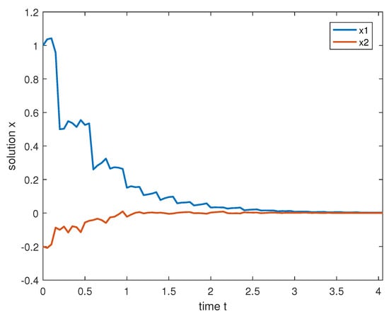
Figure 1.
The behaviors of the system (4) in Case 1.
Case 2. Let same in case 1, i.e. , , and let , then from (4), , i.e. , . This indicates that the continuous system is unstable. Letting , , we have , . To ensure that (A7) holds, namely
it is sufficient to
We can let , , , , thus . this indicate (A7) also holds. Thus, the condition in Theorem 1 is satisfied, which verifies that system Definition 1 is p-ES, and its simulation is shown in Figure 2.
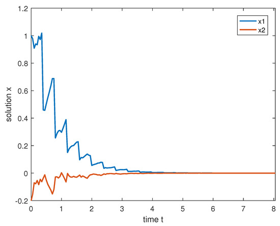
Figure 2.
The behaviors of the system (4) in Case 2.
Remark 11.
This numerical simulation example verifies the correctness of our Theorem 1. If we let , , , in Case 1, thus ; this indicates (A7) also holds. When the continuous system is stable, the system remains stable even under the influence of destabilizing periodic delayed impulses, i.e., PII . When the continuous system is unstable, stabilizing periodic delayed impulses, i.e., PII can stabilize the system.
5. Conclusions
In this paper, we have introduced the concept of periodic impulsive intensity (PII) and developed new stability criteria for the pth moment exponential stability of RIDNS with multiple periodic delayed impulses. Our results show that periodic delayed impulses can both stabilize unstable systems and destabilize stable ones, highlighting the dual effects of impulse intensity and delay length. By addressing random disturbances, time-varying delays in continuous flow, and time delays in impulsive dynamics, our approach extends previous works and removes restrictive conditions, offering greater flexibility for both deterministic and stochastic systems.
Author Contributions
Conceptualization, Q.Z. and D.R.; methodology, Y.L.; software, Y.L.; validation, Y.L., D.R. and Q.Z.; formal analysis, Y.L.; investigation, Y.L.; resources, Q.Z.; data curation, Y.L.; writing—original draft preparation, Y.L.; writing—review and editing, D.R. and Q.Z.; visualization, Y.L.; supervision, Q.Z.; project administration, Q.Z.; funding acquisition, Y.L. All authors have read and agreed to the published version of the manuscript.
Funding
This research was funded by the Natural Science Foundation of Hunan Province, China (2025JJ60047).
Data Availability Statement
No new data were created or analyzed in this study. Data sharing is not applicable to this article.
Acknowledgments
The authors would like to thank the reviewers for their valuable comments and suggestions, which helped to improve the quality of this paper.
Conflicts of Interest
The authors declare no conflict of interest.
References
- Nesic, D.; Teel, A.R. Input-output stability properties of networked control systems. IEEE Trans. Automat. Control 2004, 49, 1650–1667. [Google Scholar] [CrossRef]
- Goebel, R.; Sanfelice, R.G.; Teel, A.R. Hybrid dynamical systems. IEEE Control Syst. Mag. 2009, 29, 28–93. [Google Scholar] [CrossRef]
- Yang, T. Impulsive Control Theory; Springer: Berlin/Heidelberg, Germany, 2001. [Google Scholar]
- Zhang, J.; Nie, X. Exponential stability of fractional-order asynchronous switched impulsive systems with time delay and mode-dependent parameter uncertainty. J. Franklin. Inst. 2025, 362, 107406. [Google Scholar] [CrossRef]
- Zhang, T.; Cao, J.; Li, X.; Hua, L. Finite-time input-to-state stability and settling-time estimation of impulsive switched systems with multiple impulses. J. Franklin. Inst. 2024, 361, 107205. [Google Scholar] [CrossRef]
- Cheng, M.; Zhao, J.; Sun, Z.; Dong, Y. Finite-time stability via event-triggered delayed impulse control for time-varying nonlinear impulsive systems. J. Franklin. Inst. 2024, 361, 107152. [Google Scholar] [CrossRef]
- Aldosari, F.; Ebaid, A. Analytical and Numerical Investigation for the Inhomogeneous Pantograph Equation. Axioms 2024, 13, 377. [Google Scholar] [CrossRef]
- Albidah, A.; Kanaan, N.; Ebaid, A.; AlJeaid, H. Exact and Numerical Analysis of the Pantograph Delay Differential Equation via the Homotopy Perturbation Method. Mathematics 2023, 11, 944. [Google Scholar] [CrossRef]
- Zhang, W.; Feng, L.; Wu, Z.; Park, J. Stability criteria of random delay differential systems subject to random impulses. Internat. J. Robust Nonlinear Control 2021, 31, 6681–6698. [Google Scholar] [CrossRef]
- Ruan, D.; Lu, Y.; Zhu, Q. Generalized exponential stability of stochastic delayed systems with delayed impulses and infinite delays. Syst. Control Lett. 2025, 204, 106194. [Google Scholar] [CrossRef]
- Bertram, J.; Sarachik, P. Stability of circuits with randomly time-varying parameters. IRE Trans. Circuit Theory 1959, 5, 260–270. [Google Scholar] [CrossRef]
- Soong, T.T. Random Differential Equations in Science and Engineering; Academic Press: New York, NY, USA, 1973. [Google Scholar]
- Khasminskii, R. Stochastic Stability of Differential Equations; Springer: Berlin/Heidelberg, Germany, 1980. [Google Scholar]
- Wu, Z. Stability criteria of random nonlinear systems and their applications. IEEE Trans. Automat. Control 2015, 60, 1038–1049. [Google Scholar] [CrossRef]
- Wu, Z.; Karimi, H.; Shi, P. Practical trajectory tracking of random Lagrange systems. Automatica 2019, 105, 314–322. [Google Scholar] [CrossRef]
- Zhang, D.; Wu, Z.; Sun, X.; Wang, W. Noise-to-state stability for a class of random systems with state-dependent switching. IEEE Trans. Automat. Control 2015, 61, 3164–3170. [Google Scholar] [CrossRef]
- Zhang, H.; Xia, Y.; Wu, Z. Noise-to-state stability of random switched systems and its applications. IEEE Trans. Automat. Control 2015, 61, 1607–1612. [Google Scholar] [CrossRef]
- Yao, L.; Feng, L.; Wu, Z. Adaptive tracking control for random nonlinear system. Internat. J. Robust Nonlinear Control 2017, 27, 3833–3840. [Google Scholar] [CrossRef]
- Alyoubi, R.; Ebaid, A.; El-Zahar, E.; Aljoufi, M. A novel analytical treatment for the Ambartsumian delay differential equation with a variable coefficient. AIMS Math. 2024, 9, 35743–35758. [Google Scholar] [CrossRef]
- Tunc, O.; Berezansky, L.; Tunc, C.; Yao, J. Enhanced impulsive stabilization results of differential and integro-differential equations of second order. Discret. Contin. Dyn. Syst. Ser. B 2020. [Google Scholar] [CrossRef]
- Pinelas, S.; Tunc, O.; Korkmaz, E.; Tunc, C. Existence and stabilization for impulsive differential equations of second order with multiple delays. Electron. J. Differ. Equ. 2024, 1–18. [Google Scholar] [CrossRef]
- Feng, L.; Park, J.; Zhang, W. Improved noise-to-state stability criteria of random nonlinear systems with stochastic impulses. IET Control Theory Appl. 2021, 15, 96–109. [Google Scholar] [CrossRef]
- Feng, L.; Zhang, W.; Yang, Z.; Park, J. Further stability results for random nonlinear systems with stochastic impulses. J. Franklin. Inst. 2021, 358, 5426–5450. [Google Scholar] [CrossRef]
- Feng, L.; Zhang, W.; Wu, Z. Noise-to-state stability of random impulsive delay systems with multiple random impulses. Appl. Math. Comput. 2023, 436, 127517. [Google Scholar] [CrossRef]
- Lu, Y.; Zhu, Q. Exponential stability of impulsive random delayed nonlinear systems with average-delay impulses. J. Franklin. Inst. 2024, 361, 106813. [Google Scholar] [CrossRef]
- Li, P.; Li, X.; Lu, J. Input-to-state stability of impulsive delay systems with multiple impulses. IEEE Trans. Automat. Control 2021, 66, 362–368. [Google Scholar] [CrossRef]
- Xu, H.; Zhu, Q. Exponential stability of stochastic nonlinear delay systems subject to multiple periodic impulses. IEEE Trans. Automat. Control 2024, 69, 2621–2628. [Google Scholar] [CrossRef]
- Lu, J.; Ho, D.W.C.; Cao, J. A unified synchronization criterion for impulsive dynamical networks. Automatica 2010, 46, 1215–1221. [Google Scholar] [CrossRef]
- Jiang, B.; Lu, J.; Liu, Y. Exponential stability of delayed systems with average-delay impulses. SIAM J. Control Optim. 2020, 58, 3763–3784. [Google Scholar] [CrossRef]
- Zhou, B. On asymptotic stability of linear time-varying systems. Automatica 2016, 68, 266–276. [Google Scholar] [CrossRef]


Disclaimer/Publisher’s Note: The statements, opinions and data contained in all publications are solely those of the individual author(s) and contributor(s) and not of MDPI and/or the editor(s). MDPI and/or the editor(s) disclaim responsibility for any injury to people or property resulting from any ideas, methods, instructions or products referred to in the content. |
© 2025 by the authors. Licensee MDPI, Basel, Switzerland. This article is an open access article distributed under the terms and conditions of the Creative Commons Attribution (CC BY) license (https://creativecommons.org/licenses/by/4.0/).